1. Introduction
Mountain hazards are common natural disasters that affect human lives and property adversely [
1,
2]. In the field of hazard simulation, researchers commonly utilize the shallow water equations (SWEs) as the governing equations. These equations are applied to studying a range of hazards, including flash floods [
3,
4,
5], debris flows [
6,
7], landslides [
8], and dam breaches [
9,
10,
11]. Solving the SWEs is essential to capture the dynamics of these hazards, necessitating the development of an effective and efficient solver by model developers [
12,
13,
14].
Prominent solvers utilized for the SWEs include Massflow [
10,
15,
16,
17,
18,
19,
20], FLO2D [
21,
22,
23,
24,
25], and OpenLISEM [
26,
27,
28,
29,
30,
31,
32,
33]. Traditional numerical methods, such as finite difference [
10,
15,
34,
35] and finite volume [
36,
37], have been employed for solving partial differential equations (PDEs). These methods necessitate a deep understanding of the underlying physics and mathematical techniques involved in numerical methods for PDEs. The construction of sophisticated spatial discretization schemes presents challenges, as it is required to account for shock waves and wave propagation directions. The construction of Riemann solvers is highly intricate and demands significant theoretical expertise from modelers.
In recent years, there has been notable progress in the field of deep learning [
38,
39,
40,
41]. As a result, researchers have begun exploring the integration of deep learning with dynamic systems, although the number of studies conducted thus far remains limited [
42,
43,
44]. Solving PDEs through deep learning is an active research area in this field. Two mainstream modeling methods have emerged. The first method involves parameterizing the solution mapping using a convolutional neural network and utilizing trained networks to replace the traditional PDE solver [
45,
46,
47,
48,
49]. The second method directly parameterizes the solution function as a neural network. The difference between the first method and the second method, is that the input of the second method is not the flow field at the previous moment but is instead the independent variable of the solution function itself (such as time and space coordinates) to obtain the field of flow at the current moment [
50,
51,
52,
53,
54]. However, these pioneering deep learning methods for SWEs have limitations. They either learn a direct mapping or they directly approximate the PDE solution, necessitating the training of a new neural network for each new dataset or set of function parameters/coefficients. Consequently, capturing various variations of the terrain and stress constitutive relations becomes challenging, leading to weak generalization capabilities and therefore limiting the potential of deep learning methods for broader applications.
To achieve data-driven and theory-driven coupled flow simulation while maintaining generalization capability, we propose a hybrid method that integrates theory-driven and data-driven approaches for solving SWEs. The main idea of the model design involves utilizing neural networks to model the flux terms, thereby alleviating the modeling challenges associated with the Riemann solver. Additionally, we employ theoretical modeling techniques to address the complexities and variations presented in terrain and friction terms, ensuring the generalization capability of the SWE solver.
In this paper, we outline the structure of our research as follows. Firstly, we generate discrete sample data and employ a convolutional neural network (CNN) to learn the underlying information contained in the discrete data to implement the functionality of the Riemann solver for the resolution of flux terms. This data-driven method allows us to model the flux terms independently from the variations of the terrain and friction terms. We train the CNN by comparing its inference results with predictions of the numerical schemes. Next, by incorporating relevant computational fluid dynamics theories, we construct a solver suitable for real terrain and friction conditions. This is achieved by combining the data-driven flux term simulator with the theory-driven slope source term and friction term. By leveraging both methodologies, we address the limitations faced by previous deep learning-based solvers in capturing variations of complex terrain and stress constitutive relations. In the final phase of our study, the accuracy and stability of our proposed solver were rigorously examined across three distinct scenarios: firstly, in the presence of analytically solvable cases, followed by its application to a real-world landslide event, and lastly, a comparative assessment with the state-of-the-art solving software, Massflow. This comprehensive testing protocol was chosen to comprehensively evaluate the efficacy of the solver and to affirm its competence in faithfully replicating hazardous scenarios, particularly those characterized by intricate terrains. The model validation results demonstrate that the hybrid method, which combines theory-driven and data-driven approaches for solving the SWEs, is a feasible modeling technique. It offers significant advantages by reducing the requirements on modelers in terms of understanding the fundamental physics principles and mathematical techniques involved in the resolution of PDEs. Furthermore, it ensures the generalization capabilities on complex and variable terrains and frictions. This research introduces a new data-driven modeling perspective that holds promise for researchers in the field of land surface process simulation.
2. Governing Equations
Without consideration of Coriolis and wind force, a hyperbolic conservation law of the two-dimensional SWEs can be expressed in a matrix form as:
The vectors in the above equation are specifically expressed as:
where
is water depth from the free surface to the bed elevation
;
and
are the depth-integrated flow velocities in
and
directions, respectively;
is the momentum in
direction;
is the momentum in
direction;
g is gravitational acceleration;
and
are the slope or momentum source term in
and
directions, respectively; and
and
are the bed friction resistance term in
and
directions, respectively.
In the process of solving the SWEs, we should consider the discretization of the source term, which is composed of the slope source term and the bed friction term. The above-mentioned two terms are the main sources of momentum that are driving the fluid to move, and improper treatment of these two terms may result in conflict with the so-called “well balanced” property (or “C property”) and lead to instability and inconvergent issues which cannot be overcome, even with a large amount of computation.
The constitutive equation of stress for SWEs is as follows:
For landslides, the resistance term during motion is calculated using the Coulomb friction model which can be calculated as:
where
is the friction coefficient representing the ratio of friction force to pressure.
3. Convection Flux Term Calculation Based on the Data-Driven Method
3.1. Generation of the Training Dataset
The specific description of our data generation is as follows:
Because the flow depth data in nature generally do not exceed 100, we randomly sample the flow depth data
in the [0, 100] interval. Because the Froude number
Fr of the fluid in nature is all in 3 [
55], its calculation formula is as follows:
We randomly generate flow velocity samples in the velocity interval . The flow velocity is divided into the direction and direction. According to the flow velocity data we generated, it is evenly distributed in each direction, and the sampling interval of the velocity direction angle is [0, 2π]. and are the depth-integrated flow velocities in the and directions, respectively; is calculated based on the previously generated and , and the momentum and are calculated by the flow depth data. We randomly generate pairs of samples, and each pair is sampled in the above-mentioned way.
We use the first-order accurate upwind method to generate discrete data as the training set, and the generation procedure is described below.
We judge the windward direction according to the speed at the cell interface; the function value at the boundary is estimated as:
Referring to the ideas given by Bar-Sinai [
43], the mapping from the flow field to the discrete scheme of the derivative can be learned through a convolutional neural network.
The expression of the upwind scheme at the interface is:
and are the differential formats in the and directions. Given that, in two-dimensional SWEs, the solving of the two dimensions is consistent and symmetric, we only train for one dimension and then apply the trained parameters to the other dimension. We randomly generate 4096 random flow fields of size 1 × 2, and generate data sequences in an upwind manner.
3.2. Design of the Data-Driven Model
The constructed neural network model, including all physical constraints, is implemented using the TensorFlow framework [
56]. The model has three fully convolutional layers. The primary network layer of the convolutional neural network is the convolution layer, and the main structure is composed of multiple convolution kernels and activation functions. The convolution operation of a convolution kernel is calculated as follows:
The conv1 layer consists of six kernel filters. The conv2 layer consists of eight kernel filters and a ReLU nonlinear unit between each layer. The activation function of the last convolutional layer is the sigmoid function. Therefore, the neural network prediction at a single boundary depends on the values of the local solutions of up to two grid cells to the left and right of the maximum range, independent of the model resolution. The specific neural network structure is shown in
Figure 1.
3.3. Model Training
We trained our model using the Adam optimizer for a total of 10,000 steps. The Adam (adaptive moment estimation) optimization algorithm is basically a combination of Momentum and RMSprop. The algorithm’s paper was published at the top conference ICLR in 2015 [
57], and is the most popular optimizer in the field of deep learning. It is calculated as follows:
The Adam algorithm maintains the inertia of momentum accumulation during the iteration process through the first-order moment, and records the second-order moment of the gradient at the same time, that is, the average of the past gradient square and the current gradient square. The Adam algorithm is suitable for most non-convex optimizations, and it is also suitable for large data sets and high-dimensional spaces. It has good performance in many learning scenarios. We set the initial learning rate to 0.001. The hyperparameters and were set to 0.9 and 0.999, respectively. Here, is set to 10−8. The batch size we used was 128 times the resampling factor.
We use cross entropy as the loss function, and its calculation formula in this paper is as follows:
All of our results show models trained using a loss function based on the boundary value variables. The model was trained on an NVIDIA GeForce GTX 1070 laptop GPU, made by Nvidia in the Santa Clara, CA, United States, in less than 10 h.
3.4. The Trained Model
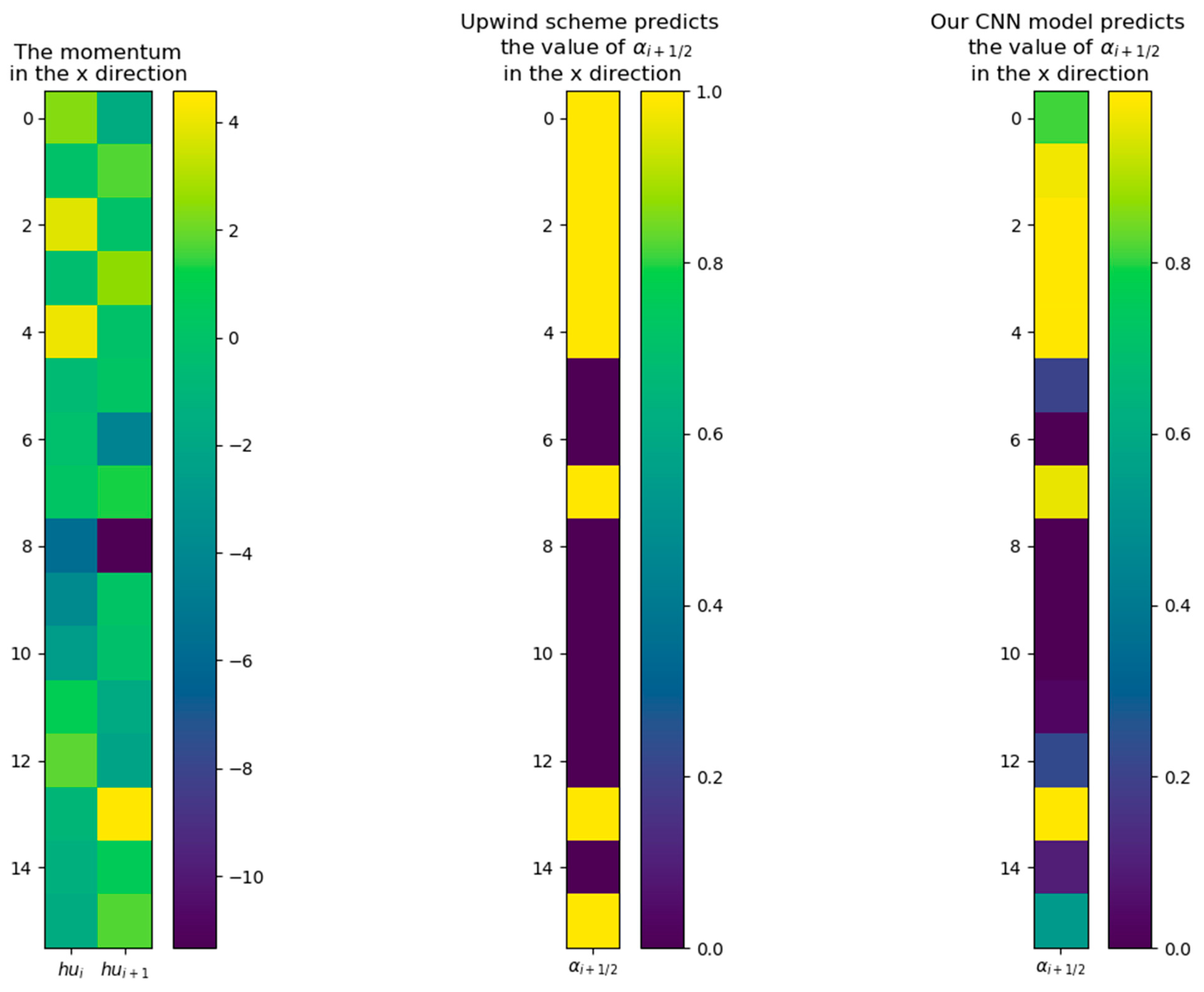
We randomly generated 4096 sets of gridded flow field data, and compared the value of
predicted by the first-order upwind scheme with the value of
predicted by our trained CNN. We randomly selected the comparison results of predicted
values generated by the upwind scheme and CNN from two sets of flow field data for display. The comparison figures of the two sets of results are shown in
Figure 2 and
Figure 3, respectively.
It can be seen from the above figures that the output of the neural network ranges from 0 to 1, which is very close to the result predicted by the first-order upwind difference scheme.
4. Construction of the Hybrid Solver
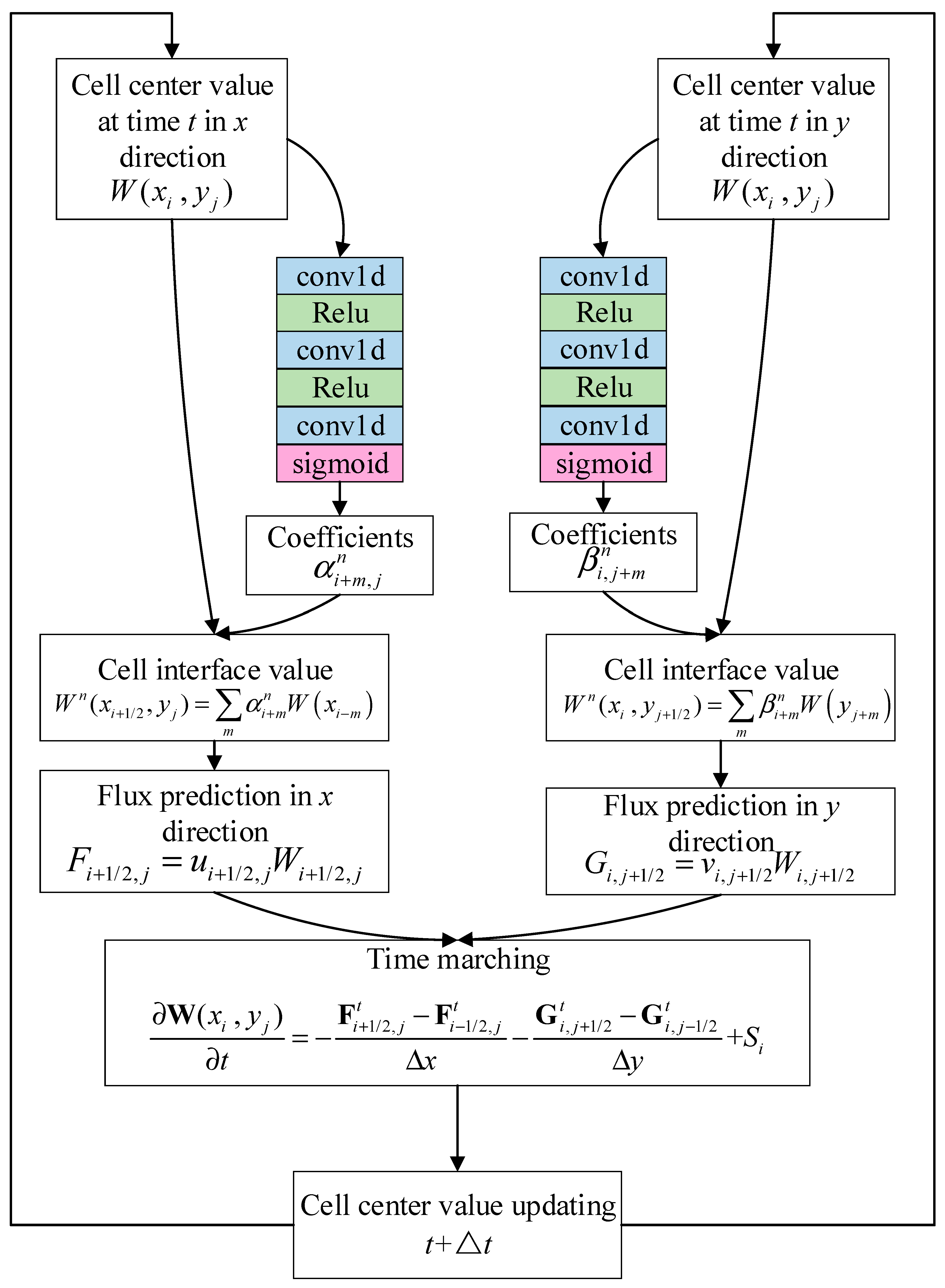
The hybrid SWE solver is composed of the following modules: time marching scheme, cell interface flux predictor, source term discretization scheme, boundary condition treatment, adaptive time step calculation, etc. Predictions in two dimensions are achieved by solvers that combine the theory and data-driven methods in two respective directions. The overall modeling framework of the hybrid solver is shown in
Figure 4.
We used the first-order Euler method for time integration and the following time marching scheme is constructed:
To ensure the numerical stability of the explicit time marching scheme, we need to guarantee that the characteristic waves do not propagate over more than one cell within a time step so that non-physical oscillations can be avoided. To adapt to time steps of different sizes under different flow velocities, we adopt the Courant–Friedrichs–Lewy (CFL) stability condition to predict the time step size:
where
Cr is the Courant number, which determines the number of grid cells that the characteristic wave transfers in a time step.
The source term is discretized by the central difference scheme, and it is calculated as follows:
where
is the mass free surface in the
i-th column and
j-th row;
and
are the slope or momentum source term in
and
directions, respectively;
g is the gravitational acceleration; and
is the water depth from the free surface to the bed elevation
in the
i-th column and
j-th row.
Under complex terrain conditions, it is common for some grid cells to contain fluid while their adjacent cells do not. Without correctly considering this situation, directly discretizing the source term will lead to physical errors such as non-physical flow and negative water depth, resulting in an unstable solution. To prevent non-physical oscillations and enable the solver to handle complex terrains, it is crucial to address the treatment of the dry–wet boundary [
58,
59,
60].
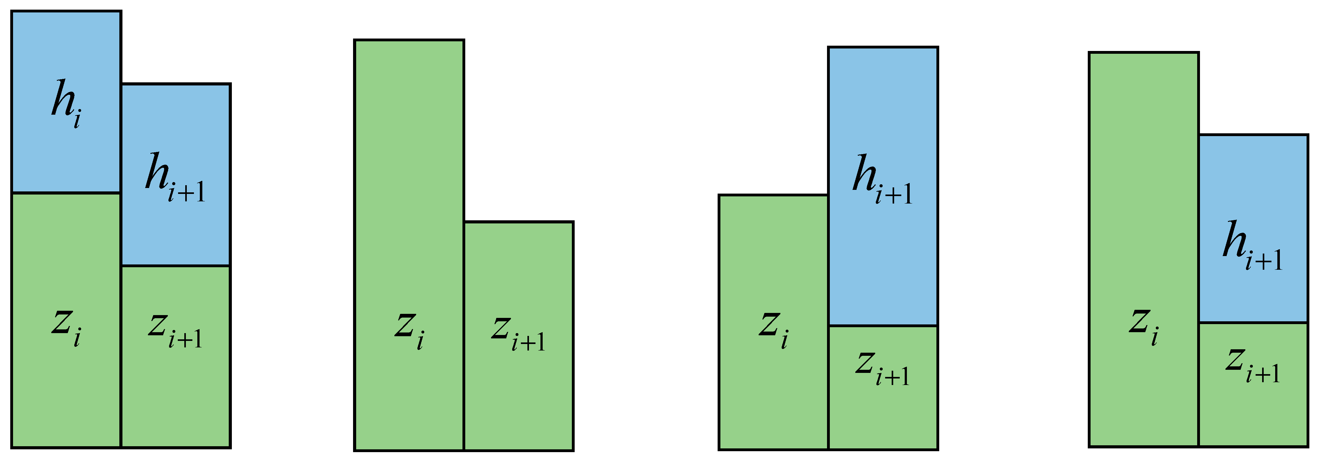
As shown in
Figure 5, there are four scenarios that can occur between two grids; these include: (1) both grids are wet (2) both grids are dry, (3) one grid is dry and the other is wet with the free surface of the wet grid higher than the dry grid, (4) one grid is dry and the other is wet with the free surface of the wet grid lower than the dry grid.
Additional processing should be assigned to some of the above-mentioned scenarios. The first scenario, which involves a normal pressure difference due to an uneven free surface, does not require any additional processing. Similarly, the second scenario, where there is no fluid in the grid and the flow depth is 0, also does not require extra processing since the source term is 0. The third scenario, where the free surface is higher than the dry grid and there is a normal pressure difference, does not need additional processing either. However, for the fourth scenario, where the free surface is lower than the dry terrain, direct application of the center difference scheme for discretization of the free surface can result in a false pressure difference from the dry grid to the wet grid. This false pressure difference directly affects the stability and conservation during the solution process. Consequently, it is necessary to address the issue of false pressure difference in the fourth scenario.
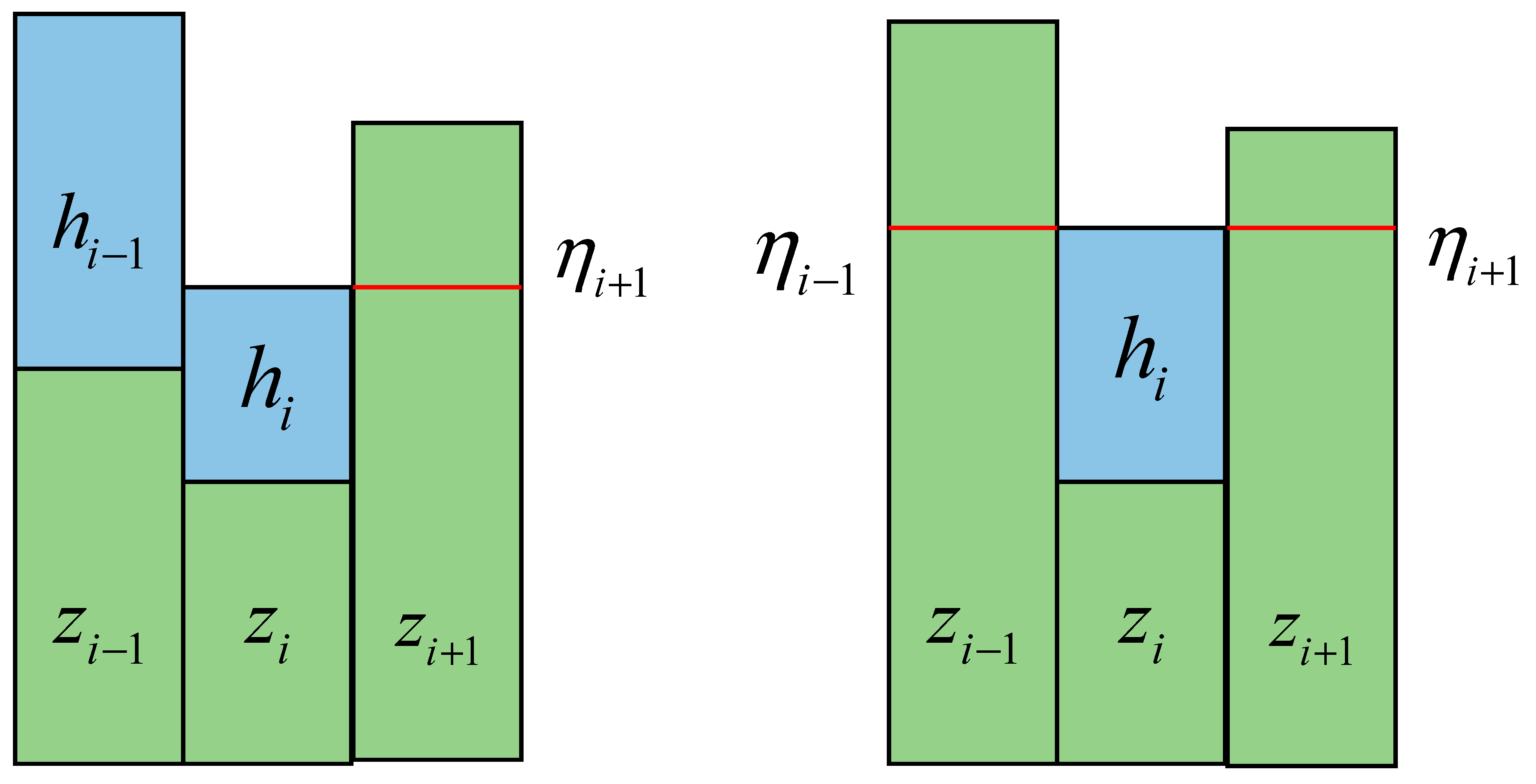
To ensure the stability of the solution process, it is necessary to address the issue of false mass pressure difference and non-physical momentum that arises when a dry grid is higher than the free mass surface. In order to correct this error, we employ the reconstruction method, as depicted in
Figure 6. The reconstruction calculation formula of mass free surface is as follows:
This method involves eliminating the gradient between the high dry grid and the free surface during the differencing process of the high dry grid. Specifically, when calculating the source term of the central grid, we will reconstruct the elevation of the dry grid adjacent to the free surface, ensuring that it is equal to the free surface. This reconstruction ensures that there is no gradient difference between the two grids, effectively eliminating any potential false momentum.
5. Model Validation
5.1. Comparison with the Analytical Solution Results
We chose a one-dimensional smooth bed dam break flow simulation case to verify the stability of the solver in the shock region, and compared it with the analytical solution. This analytical solution is a classic example, and its water depth analytical form is mainly divided into three parts:
h represents the initial water depth of the upstream, the upstream and downstream take
x = 1 as the dividing line,
t represents the evolution time from the start of the collapse, and the analytical formula of the velocity is:
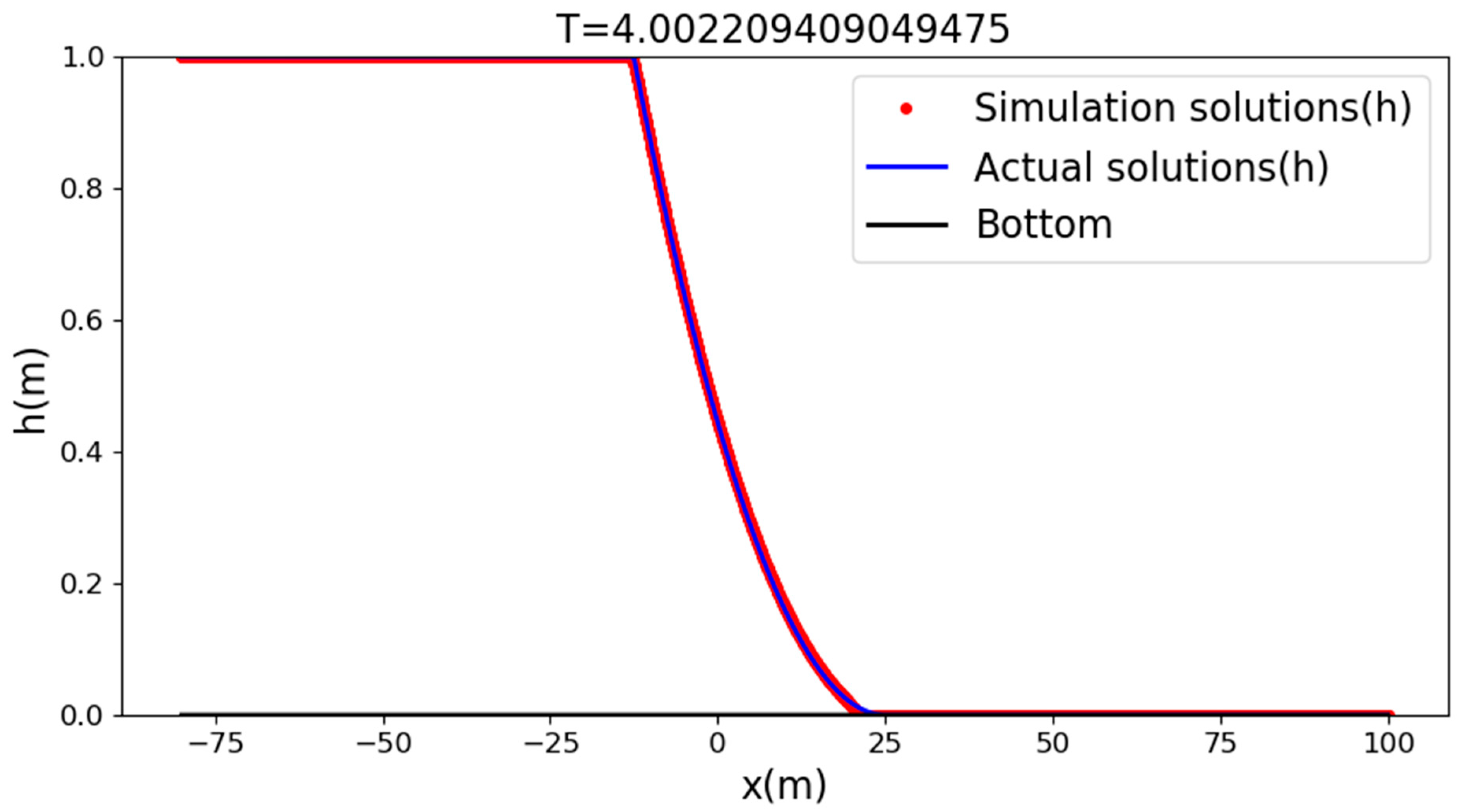
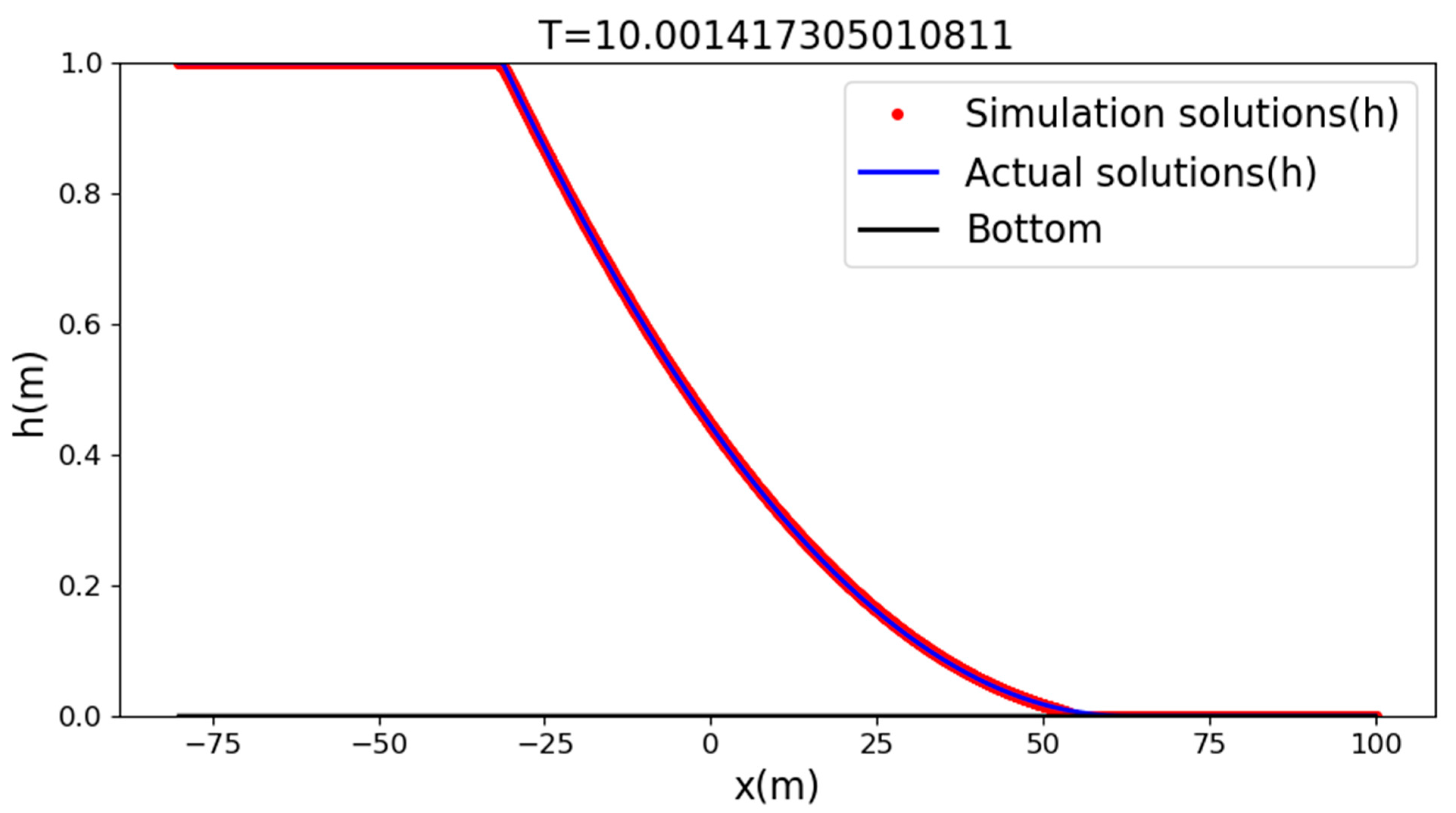
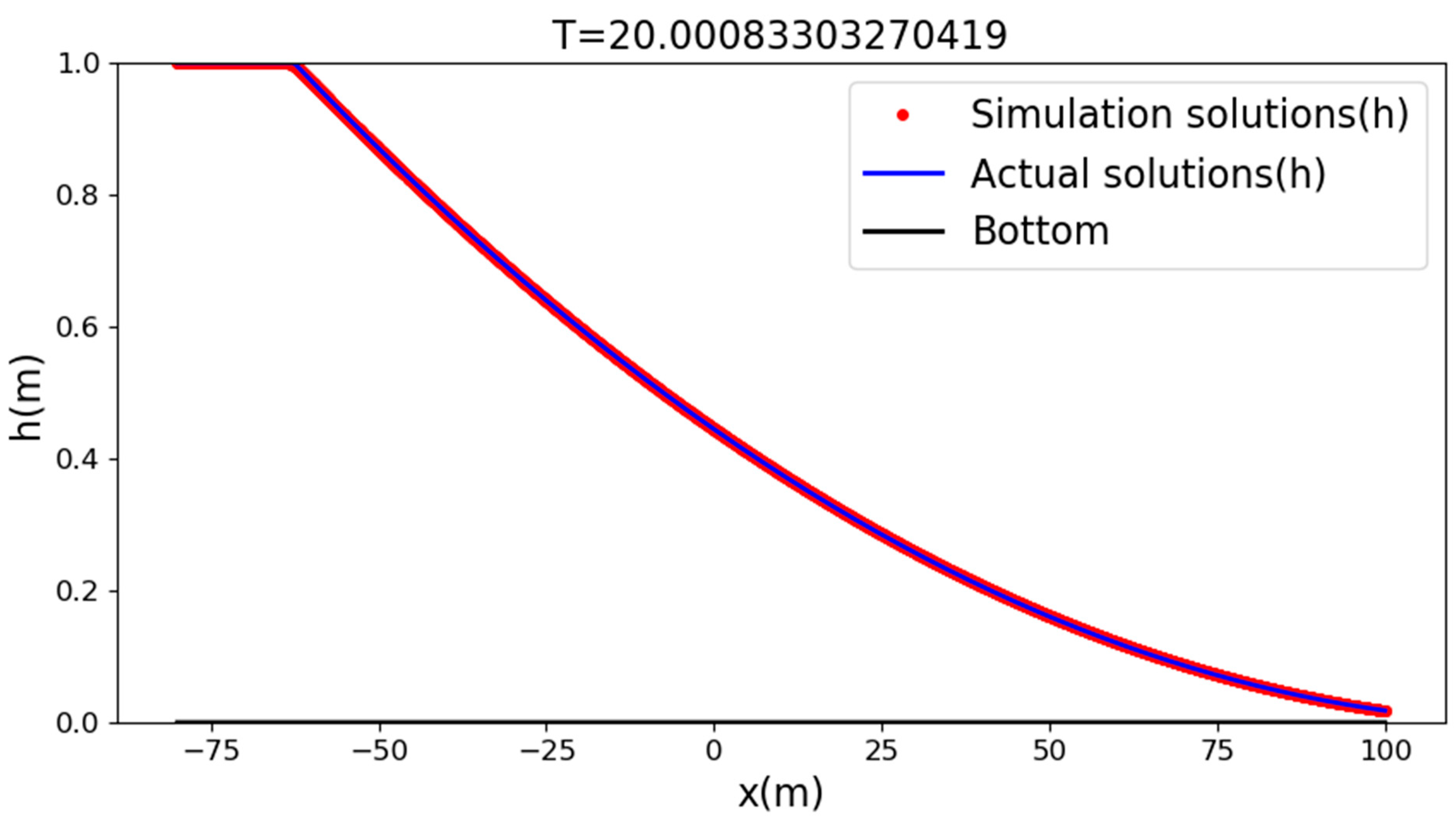
The case we set up was a rectangular river channel with a length of 180 m and 80 m width of water, with a depth of 1 m in the upstream, simulating an instantaneous collapse state. The grid size dx was 0.05 m, and the simulation results using the solver proposed(
Figure 7,
Figure 8 and
Figure 9) in this paper were as follows:
The RMSE of the simulation results of our proposed solver was about 7.58 × 10⁻⁶, and the MAE of the simulation results of our proposed solver was about 0.004. From the above figure, we can see that the solver we propose can guarantee the stability well in the shock wave environment, and the format constructed in this paper can guarantee the high precision of the solution.
5.2. Comparison of Solver Simulation Results with Real Landslide Cases
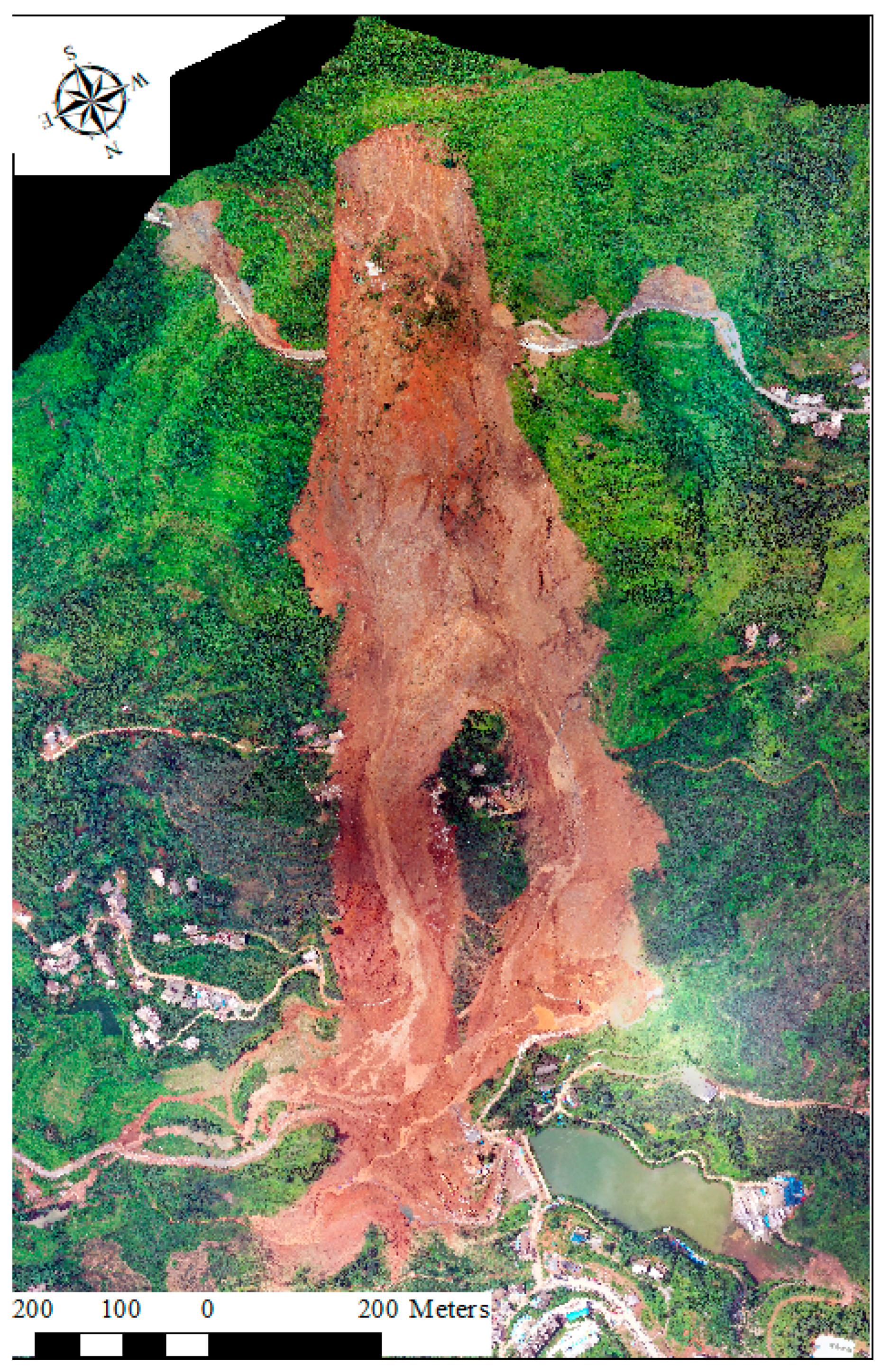
On 23 July 2019, a large-scale landslide occurred in Jichang town, Shuicheng County, Liupanshui City, Guizhou Province, China, resulting in a deposit volume of approximately 2 × 10
6 m
3. This catastrophic event led to the destruction of 22 houses, claiming the lives of 42 people, with nine individuals reported as missing. In this study, we utilized simulation data obtained from Guo [
34] for our analysis. This case serves as a case study to assess both the stability and generalization capabilities of the proposed hybrid SWE solver (
Figure 10).
In our study, we applied our novel solver to simulate the Jichang Town landslide, a real-world case. The simulation results demonstrated a remarkable level of agreement with the actual landslide, validating the robustness and accuracy of our solver in practical scenarios. This significant alignment between the simulated and real events reinforces the applicability and reliability of our solver for real-world landslide prediction and hazard assessment.
We complemented our simulation findings by presenting compelling visual evidence. Our side-by-side comparison included on-site drone photographs capturing the actual landslide, juxtaposed with images illustrating the results of our simulation. This visual comparison highlighted the striking resemblance between the two, further affirming the precision and effectiveness of our solver in closely mirroring real-world landslide occurrences (
Figure 11).
The successful application of our solver to a real landslide case, coupled with the strong alignment between the simulated and actual events, underscores the potential of our approach for accurate hazard dynamics prediction. This achievement opens up promising avenues for enhancing our understanding of landslide behavior and aiding in the development of effective mitigation strategies in the face of such natural hazards.
5.3. Model Application in Woda Town Landslide
The Woda town landslide, which is situated upstream of the Jinsha River in the eastern region of the Qinghai–Tibet Plateau in southwestern China, has been extensively studied, monitored, and simulated [
61,
62]. In this study, we utilized simulation data obtained from Liu and He [
63] for our analysis. The total flood volume considered in the simulations was approximately 2.9 × 10
7 m
3. We employed the Coulomb friction model as the stress constitutive model, with a friction coefficient of 0.3 as suggested by Liu and He [
63].
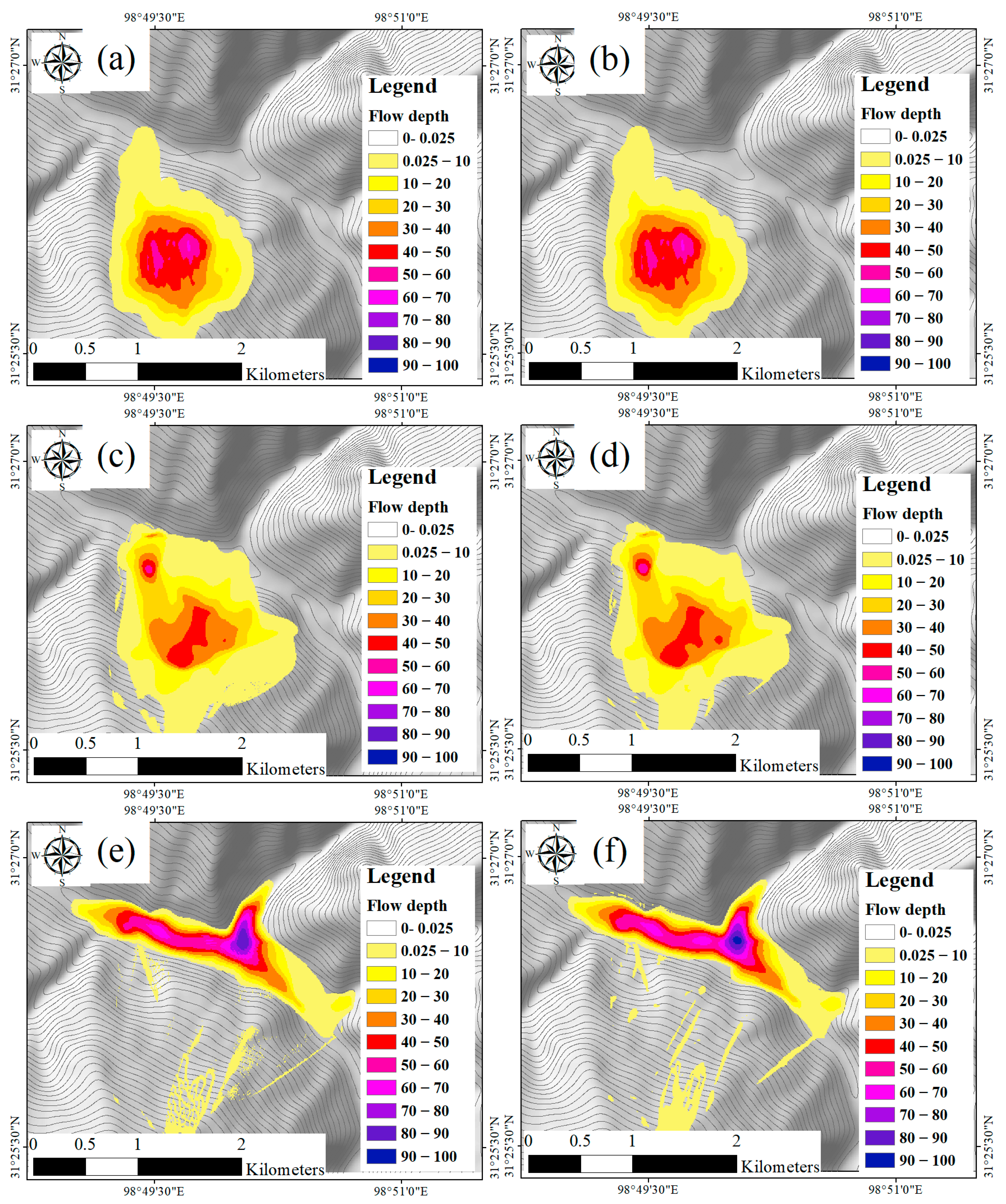
Figure 12 presents a comprehensive comparison between the simulation results obtained using the solver proposed in this paper and the widely recognized mountain disaster simulation software, Massflow, under real-world terrain conditions. The simulation results obtained from the proposed solver exhibited a high degree of congruence with the outcomes derived from Massflow simulations, particularly in terms of the extent of inundation and the distribution of flow depths.
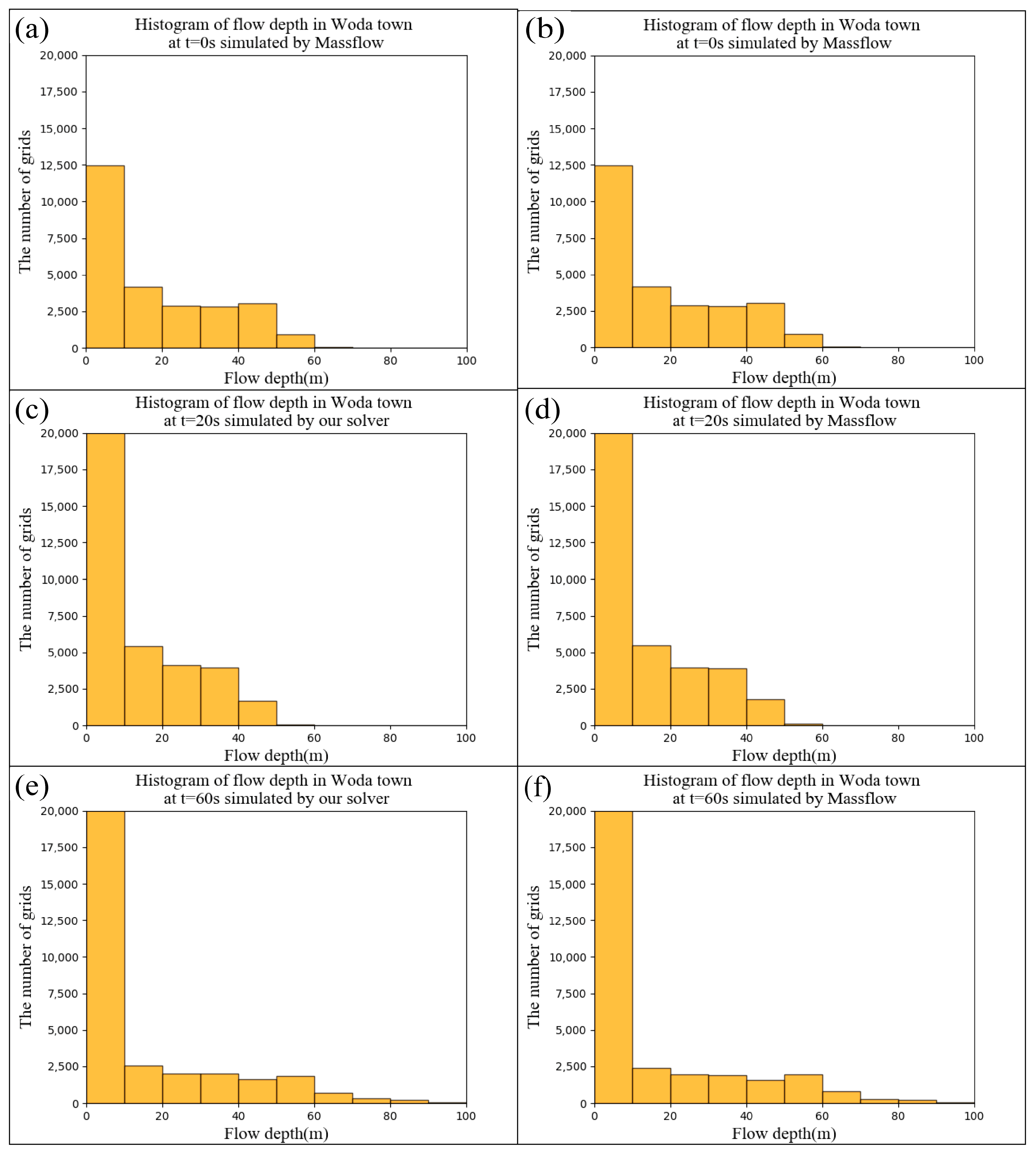
Figure 13 illustrates the flow depth histogram derived from the simulation results obtained using the Massflow and the proposed solver. The histogram provides a frequency distribution of the flow depth values obtained in the simulation results. In the
x-axis of
Figure 13, flow depth is represented in meters, while the
y-axis indicates the number of grid cells associated with each flow depth value. The histogram distribution demonstrates a striking similarity between the simulation results of the two models.
The Woda landslide simulation results of the proposed solver are close to those of the Massflow solver. The histogram distribution of the flow depth demonstrated a remarkable similarity between the two solvers, indicating that the proposed solver exhibits reliable performance in simulating landslide dynamics in various realistic terrains.
6. Discussion and Conclusions
This study presents a novel approach for constructing the SWE solver by combining theory and data-driven methodologies. The proposed method leverages neural networks to replace the functionality of the convection flux solver, simplifying the modeling process of the SWE solver. Additionally, theoretical modeling techniques are employed to handle complex and diverse terrains and friction stress, ensuring the solver’s generalization capability. By comparing the simulation results with analytical solutions, real-world landslide cases, and the simulation software Massflow, this study validates the advanced capability of our proposed solver in accurately simulating hazardous scenarios. The main contributions and innovations of this study can be summarized as follows:
(1) Introduction of a deep learning method for the construction of the SWE solver: We propose a novel data-driven spatial discretization method that utilizes convolutional neural networks to learn fluid flux computations. This approach reduces the complexity associated with traditional numerical methods such as flux discretization schemes and Riemann solvers. Consequently, it simplifies the modeling process and lowers the theoretical knowledge requirements of solver developers.
(2) Adoption of a hybrid method combining theoretical and data-driven modeling: By combining the predicted flux from neural networks with relevant computational fluid dynamics theories, the proposed model enables the solver to utilize the advantages of the data-driven flux solver while adapting to real-world terrain conditions, therefore ensuring both the generalization capability and the physical reasonableness. The proposed model overcomes limitations encountered in previous DL-based SWE solvers, allowing our solver to capture complex terrains and variations in stress constitutive properties without requiring the retraining of neural networks for new terrain or friction conditions.
(3) Evaluation of the proposed solver’s performance is based on two real mountain landslide cases: Through comparison with the widely used simulation software, Massflow, simulation results demonstrated the stable performance of the proposed solver under complex terrain conditions. The simulation outcomes closely aligned with those obtained from the Massflow software, affirming the advanced capabilities of our solver in accurately simulating hazard scenarios. These findings provide evidence of the solver’s generalization capability in addressing problems encountered in complex and varying terrains.
The deep learning-based SWE solver presented in this study introduces a new perspective for modeling hazard dynamics through data-driven approaches. It overcomes the limitations and challenges associated with traditional numerical methods and previous deep learning-based modeling techniques. This study serves as a valuable attempt and exemplar in utilizing deep learning for solving PDEs. However, it is important to acknowledge certain limitations:
(1) The study employs the first-order Euler method as the time integration scheme, which may impact the solver’s temporal accuracy. Future research should consider exploring higher-order and more stable time integration methods to enhance the solver’s temporal accuracy of the time marching scheme.
(2) The study utilizes fixed-size and shaped convolutional kernels to learn the fluid flux solver, which may restrict the neural network’s ability to capture various flow field characteristics. Further investigations can explore more flexible and adaptive convolutional kernel structures to improve the network’s adaptability and expressive power in handling diverse flow field situations.
(3) The neural network is trained using artificially generated random flow field data, which may lead to overfitting or underfitting issues when dealing with real-world flow field data. Future research can incorporate a broader range of real-world flow field data, ensuring the training process incorporates more abundant and diverse examples. This approach will enhance the performance and robustness of the neural network in generalizing to real-world flow field scenarios.
In summary, this research paper contributes to the field of hazard dynamics simulation by introducing a novel DL-based SWE solver. The combination of theory-based and data-driven methodologies enhances the solver’s capabilities in accurately simulating hazard scenarios in complex terrains. The limitations highlighted pave the way for future research to explore higher-order time integration methods, flexible convolutional kernel structures, and richer real-world flow field data. By addressing these limitations, the proposed solver can further advance the accuracy, efficiency, and generalization capabilities of hazard dynamics simulations, opening up new possibilities for research in this domain.
Author Contributions
Conceptualization, S.Y. and G.K.; methodology, S.Y. and J.T.; software, S.Y.; validation, S.Y.; formal analysis, S.Y.; investigation, J.G.; resources, S.Y. and G.K.; data curation, D.C., J.G. and H.J.; writing—original draft preparation, S.Y. and G.K.; writing—review and editing, S.Y. and G.K.; visualization, S.Y.; supervision, G.K.; project administration, C.L., J.T. and G.K.; funding acquisition, C.L. All authors have read and agreed to the published version of the manuscript.
Funding
This research was funded by National Key Research Program (2019YFC1510603); IWHR Research and Development Support Program: JZ0199A032021; GHFUND A No. ghfund202302018283; Open Research Fund of Beijing Key Laboratory of Urban Hydrological Cycle and Sponge City Technology: HYD2020OF02. National Natural Science Foundation of China: Grant No. U21A2008.
Data Availability Statement
Not applicable.
Acknowledgments
The authors also thank the anonymous reviewers for their helpful comments and suggestions.
Conflicts of Interest
The authors declare that they have no known competing financial interest or personal relationships that could have appeared to influence the work reported in this paper.
References
- Liu, D.; Cui, Y.; Wang, H.; Jin, W.; Wu, C.; Bazai, N.A.; Zhang, G.; Carling, P.A.; Chen, H. Assessment of local outburst flood risk from successive landslides: Case study of Baige landslide-dammed lake, upper Jinsha river, eastern Tibet. J. Hydrol. 2021, 599, 126294. [Google Scholar] [CrossRef]
- Yan, Y.; Cui, Y.; Liu, D.; Tang, H.; Li, Y.; Tian, X.; Zhang, L.; Hu, S. Seismic signal characteristics and interpretation of the 2020 “6.17” Danba landslide dam failure hazard chain process. Landslides 2021, 18, 2175–2192. [Google Scholar] [CrossRef]
- Kan, G.; Yao, C.; Li, Q.; Li, Z.; Yu, Z.; Liu, Z.; Ding, L.; He, X.; Liang, K. Improving event-based rainfall-runoff simulation using an ensemble artificial neural network based hybrid data-driven model. Stoch. Environ. Res. Risk Assess. 2015, 29, 1345–1370. [Google Scholar] [CrossRef]
- Kan, G.; He, X.; Ding, L.; Li, J.; Hong, Y.; Zuo, D.; Ren, M.; Lei, T.; Liang, K. Fast hydrological model calibration based on the heterogeneous parallel computing accelerated shuffled complex evolution method. Eng. Optim. 2017, 50, 106–119. [Google Scholar] [CrossRef]
- Kan, G.; Li, J.; Zhang, X.; Ding, L.; He, X.; Liang, K.; Jiang, X.; Ren, M.; Li, H.; Wang, F. A new hybrid data-driven model for event-based rainfall–runoff simulation. Neural Comput. Appl. 2017, 28, 2519–2534. [Google Scholar] [CrossRef]
- Shunyu, Y.; Bazai, N.A.; Jinbo, T.; Hu, J.; Shujian, Y.; Qiang, Z.; Ahmed, T.; Jian, G. Dynamic process of a typical slope debris flow: A case study of the wujia gully, Zengda, Sichuan Province, China. Nat. Hazards 2022, 112, 565–586. [Google Scholar] [CrossRef]
- Yan, Y.; Tang, H.; Hu, K.; Turowski, J.M.; Wei, F. Deriving Debris-Flow Dynamics From Real-Time Impact-Force Measurements. J. Geophys. Res. Earth Surf. 2023, 128, e2022JF006715. [Google Scholar] [CrossRef]
- Yan, Y.; Cui, Y.; Huang, X.; Zhang, W.; Yin, S.; Zhou, J.; Hu, S. Combining seismic signal dynamic inversion and numerical modeling improves landslide process reconstruction. EGUsphere 2022, 10, 1233–1252. [Google Scholar] [CrossRef]
- Cao, Z.; Pender, G.; Wallis, S.; Carling, P. Computational Dam-Break Hydraulics over Erodible Sediment Bed. J. Hydraul. Eng. 2004, 130, 689–703. [Google Scholar] [CrossRef]
- Ouyang, C.; He, S.; Xu, Q. MacCormack-TVD Finite Difference Solution for Dam Break Hydraulics over Erodible Sediment Beds. J. Hydraul. Eng. 2015, 141, 06014026. [Google Scholar] [CrossRef]
- Bazai, N.A.; Cui, P.; Carling, P.A.; Wang, H.; Hassan, J.; Liu, D.; Zhang, G.; Wen, J. Increasing glacial lake outburst flood hazard in response to surge glaciers in the Karakoram. Earth-Sci. Rev. 2020, 212, 103432. [Google Scholar] [CrossRef]
- Touma, R. Central unstaggered finite volume schemes for hyperbolic systems: Applications to unsteady shallow water equations. Appl. Math. Comput. 2009, 213, 47–59. [Google Scholar] [CrossRef]
- Murillo, J.; Navas-Montilla, A. A comprehensive explanation and exercise of the source terms in hyperbolic systems using Roe type solutions. Application to the 1D-2D shallow water equations. Adv. Water Resour. 2016, 98, 70–96. [Google Scholar] [CrossRef]
- Ricchiuto, M. Contributions to the Development of Residual Discretizations for Hyperbolic Conservation Laws with Application to Shallow Water Flows; Université Sciences et Technologies-Bordeaux I: Gradignan, France, 2011. [Google Scholar]
- Ouyang, C.; He, S.; Xu, Q.; Luo, Y.; Zhang, W. A MacCormack-TVD finite difference method to simulate the mass flow in mountainous terrain with variable computational domain. Comput. Geosci. 2013, 52, 1–10. [Google Scholar] [CrossRef]
- Ouyang, C.; He, S.; Tang, C. Numerical analysis of dynamics of debris flow over erodible beds in Wenchuan earthquake-induced area. Eng. Geol. 2015, 194, 62–72. [Google Scholar] [CrossRef]
- Ouyang, C.; Wang, Z.; An, H.; Liu, X.; Wang, D. An example of a hazard and risk assessment for debris flows—A case study of Niwan Gully, Wudu, China. Eng. Geol. 2019, 263, 105351. [Google Scholar] [CrossRef]
- Ouyang, C.; An, H.; Zhou, S.; Wang, Z.; Su, P.; Wang, D.; Cheng, D.; She, J. Insights from the failure and dynamic characteristics of two sequential landslides at Baige village along the Jinsha River, China. Landslides 2019, 16, 1397–1414. [Google Scholar] [CrossRef]
- Ouyang, C.; Zhou, K.; Xu, Q.; Yin, J.; Peng, D.; Wang, D.; Li, W. Dynamic analysis and numerical modeling of the 2015 catastrophic landslide of the construction waste landfill at Guangming, Shenzhen, China. Landslides 2016, 14, 705–718. [Google Scholar] [CrossRef]
- Iverson, R.M.; Ouyang, C. Entrainment of bed material by Earth-surface mass flows: Review and reformulation of depth-integrated theory. Rev. Geophys. 2015, 53, 27–58. [Google Scholar] [CrossRef]
- Rickenmann, D.; Laigle, D.; McArdell, B.W.; Hübl, J. Comparison of 2D debris-flow simulation models with field events. Comput. Geosci. 2006, 10, 241–264. [Google Scholar] [CrossRef]
- Peng, S.-H.; Lu, S.-C. FLO-2D simulation of mudflow caused by large landslide due to extremely heavy rainfall in southeastern Taiwan during Typhoon Morakot. J. Mt. Sci. 2013, 10, 207–218. [Google Scholar] [CrossRef]
- Neglia, F.; Sulpizio, R.; Dioguardi, F.; Capra, L.; Sarocchi, D. Shallow-water models for volcanic granular flows: A review of strengths and weaknesses of TITAN2D and FLO2D numerical codes. J. Volcanol. Geotherm. Res. 2021, 410, 107146. [Google Scholar] [CrossRef]
- Nocentini, M.; Tofani, V.; Gigli, G.; Fidolini, F.; Casagli, N. Modeling debris flows in volcanic terrains for hazard mapping: The case study of Ischia Island (Italy). Landslides 2014, 12, 831–846. [Google Scholar] [CrossRef]
- Luppichini, M.; Favalli, M.; Isola, I.; Nannipieri, L.; Giannecchini, R.; Bini, M. Influence of Topographic Resolution and Accuracy on Hydraulic Channel Flow Simulations: Case Study of the Versilia River (Italy). Remote Sens. 2019, 11, 1630. [Google Scholar] [CrossRef]
- Pratomo, R.A. Sensitivity analysis of flash-flood modelling in Grenada, as a small island Caribbean states. AIP Conf. Proc. 2016, 1730, 070002. [Google Scholar]
- Pérez-Molina, E.; Sliuzas, R.; Flacke, J.; Jetten, V. Developing a cellular automata model of urban growth to inform spatial policy for flood mitigation: A case study in Kampala, Uganda. Comput. Environ. Urban Syst. 2017, 65, 53–65. [Google Scholar] [CrossRef]
- Van den Bout, B.; Lombardo, L.; Chiyang, M.; van Westen, C.; Jetten, V. Physically-based catchment-scale prediction of slope failure volume and geometry. Eng. Geol. 2021, 284, 105942. [Google Scholar] [CrossRef]
- Bout, B.; Lombardo, L.; van Westen, C.J.; Jetten, V.G. Integration of two-phase solid fluid equations in a catchment model for flashfloods, debris flows and shallow slope failures. Environ. Model. Softw. 2018, 105, 1–16. [Google Scholar] [CrossRef]
- van den Bout, B.; van Asch, T.; Hu, W.; Tang, C.X.; Mavrouli, O.; Jetten, V.G.; van Westen, C.J. Towards a model for structured mass movements: The OpenLISEM hazard model 2.0a. Geosci. Model Dev. 2021, 14, 1841–1864. [Google Scholar] [CrossRef]
- Pratomo, R.A.; Jetten, V.; Alkema, D. A comparison of flash flood response at two different watersheds in Grenada, Caribbean Islands. IOP Conf. Ser. Earth Environ. Sci. 2016, 29, 012004. [Google Scholar] [CrossRef]
- Bout, B.; Jetten, V.G. The validity of flow approximations when simulating catchment-integrated flash floods. J. Hydrol. 2018, 556, 674–688. [Google Scholar] [CrossRef]
- Umer, Y.M.; Jetten, V.G.; Ettema, J. Sensitivity of flood dynamics to different soil information sources in urbanized areas. J. Hydrol. 2019, 577, 123945. [Google Scholar] [CrossRef]
- Guo, J.; Yi, S.; Yin, Y.; Cui, Y.; Qin, M.; Li, T.; Wang, C. The effect of topography on landslide kinematics: A case study of the Jichang town landslide in Guizhou, China. Landslides 2020, 17, 959–973. [Google Scholar] [CrossRef]
- Shen, W.; Li, T.; Li, P.; Guo, J. A modified finite difference model for the modeling of flowslides. Landslides 2018, 15, 1577–1593. [Google Scholar] [CrossRef]
- Bai, X.; He, S. Dynamic process of the massive Aru glacier collapse in Tibet. Landslides 2020, 17, 1353–1361. [Google Scholar] [CrossRef]
- Denlinger, R.P.; Iverson, R.M. Granular avalanches across irregular three-dimensional terrain: 1. Theory and computation. J. Geophys. Res. Earth Surf. 2004, 109. [Google Scholar] [CrossRef]
- LeCun, Y.; Bengio, Y.; Hinton, G. Deep learning. Nature 2015, 521, 436–444. [Google Scholar] [CrossRef]
- Marx, V. The big challenges of big data. Nature 2013, 498, 255–260. [Google Scholar] [CrossRef]
- Reichstein, M.; Camps-Valls, G.; Stevens, B.; Jung, M.; Denzler, J.; Carvalhais, N.; Prabhat. Deep learning and process understanding for data-driven Earth system science. Nature 2019, 566, 195–204. [Google Scholar] [CrossRef]
- Jordan, M.I.; Mitchell, T.M. Machine learning: Trends, perspectives, and prospects. Science 2015, 349, 255–260. [Google Scholar] [CrossRef]
- Tompson, J.; Schlachter, K.; Sprechmann, P.; Perlin, K. Accelerating eulerian fluid simulation with convolutional networks. In Proceedings of the International Conference on Machine Learning, Sydney, NSW, Australia, 6–11 August 2017; pp. 3424–3433. [Google Scholar]
- Bar-Sinai, Y.; Hoyer, S.; Hickey, J.; Brenner, M.P. Learning data-driven discretizations for partial differential equations. Proc. Natl. Acad Sci. USA 2019, 116, 15344–15349. [Google Scholar] [CrossRef] [PubMed]
- Kochkov, D.; Smith, J.A.; Alieva, A.; Wang, Q.; Brenner, M.P.; Hoyer, S. Machine learning-accelerated computational fluid dynamics. Proc. Natl. Acad Sci. USA 2021, 118, e2101784118. [Google Scholar] [CrossRef]
- Khoo, Y.; Lu, J.; Ying, L. Solving parametric PDE problems with artificial neural networks. Eur. J. Appl. Math. 2021, 32, 421–435. [Google Scholar] [CrossRef]
- Adler, J.; Öktem, O. Solving ill-posed inverse problems using iterative deep neural networks. Inverse Probl. 2017, 33, 124007. [Google Scholar] [CrossRef]
- Bhatnagar, S.; Afshar, Y.; Pan, S.; Duraisamy, K.; Kaushik, S. Prediction of aerodynamic flow fields using convolutional neural networks. Comput. Mech. 2019, 64, 525–545. [Google Scholar] [CrossRef]
- Guo, X.; Li, W.; Iorio, F. Convolutional neural networks for steady flow approximation. In Proceedings of the 22nd ACM SIGKDD International Conference on Knowledge Discovery and Data Mining, San Francisco, CA, USA, 13–17 August 2016; pp. 481–490. [Google Scholar]
- Zhu, Y.; Zabaras, N. Bayesian deep convolutional encoder–decoder networks for surrogate modeling and uncertainty quantification. J. Comput. Phys. 2018, 366, 415–447. [Google Scholar] [CrossRef]
- Bar, L.; Sochen, N. Unsupervised deep learning algorithm for PDE-based forward and inverse problems. arXiv 2019, arXiv:1904.05417. [Google Scholar]
- Pan, S.; Duraisamy, K. Physics-informed probabilistic learning of linear embeddings of nonlinear dynamics with guaranteed stability. SIAM J. Appl. Dyn. Syst. 2020, 19, 480–509. [Google Scholar] [CrossRef]
- Raissi, M.; Perdikaris, P.; Karniadakis, G.E. Physics-informed neural networks: A deep learning framework for solving forward and inverse problems involving nonlinear partial differential equations. J. Comput. Phys. 2019, 378, 686–707. [Google Scholar] [CrossRef]
- Smith, J.D.; Azizzadenesheli, K.; Ross, Z.E. Eikonet: Solving the eikonal equation with deep neural networks. IEEE Trans. Geosci. Remote Sens. 2020, 59, 10685–10696. [Google Scholar] [CrossRef]
- Yu, B. The deep Ritz method: A deep learning-based numerical algorithm for solving variational problems. Commun. Math. Stat. 2018, 6, 1–12. [Google Scholar]
- Smith, J.D. Stability of a sand bed subjected to a shear flow of low Froude number. J. Geophys. Res. 1970, 75, 5928–5940. [Google Scholar] [CrossRef]
- Abadi, M.; Barham, P.; Chen, J.; Chen, Z.; Davis, A.; Dean, J.; Devin, M.; Ghemawat, S.; Irving, G.; Isard, M. Tensorflow: A system for large-scale machine learning. In Proceedings of the 12th USENIX Symposium on Operating Systems Design and Implementation (OSDI 16), Savannah, GA, USA, 2–4 November 2016; pp. 265–283. [Google Scholar]
- Kingma, D.P.; Ba, J. Adam: A method for stochastic optimization. arXiv 2014, arXiv:1412.6980. [Google Scholar]
- Kan, G.; He, X.; Li, J.; Ding, L.; Hong, Y.; Zhang, H.; Liang, K.; Zhang, M. Computer aided numerical methods for hydrological model calibration: An overview and recent development. Arch. Comput. Methods Eng. 2019, 26, 35–59. [Google Scholar] [CrossRef]
- Kan, G.; Lei, T.; Liang, K.; Li, J.; Ding, L.; He, X.; Yu, H.; Zhang, D.; Zuo, D.; Bao, Z. A multi-core CPU and many-core GPU based fast parallel shuffled complex evolution global optimization approach. IEEE Trans. Parallel Distrib. Syst. 2016, 28, 332–344. [Google Scholar] [CrossRef]
- Liu, D.; Tang, J.; Wang, H.; Cao, Y.; Bazai, N.A.; Chen, H.; Liu, D. A New Method for Wet-Dry Front Treatment in Outburst Flood Simulation. Water 2021, 13, 221. [Google Scholar] [CrossRef]
- Li, B.; Jiang, W.; Li, Y.; Luo, Y.; Jiao, Q.; Wang, X.; Zhang, J. Comparison of different atmospheric phase screen correction models in ground-based radar interferometry for landslide and open-pit mine monitoring. Int. J. Remote Sens. 2021, 42, 5925–5942. [Google Scholar] [CrossRef]
- Li, B.; Jiang, W.; Li, Y.; Luo, Y.; Qian, H.; Wang, Y.; Jiao, Q.; Zhang, Q.; Zhou, Z.; Zhang, J. Monitoring and analysis of Woda landslide stability (China) combined with InSAR, GNSS and meteorological data. Nat. Hazards Earth Syst. Sci. Discuss. 2021, 2021, 1–23. [Google Scholar]
- Liu, W.; He, S. Numerical Simulation of the Evolution Process of Disaster Chain Induced by Potential Landslide in Woda of Jinsha River Basin. Adv. Eng. Sci. 2020, 52, 38–46. [Google Scholar] [CrossRef]
Figure 1.
Data-driven spatial discretization based on deep learning.
Figure 1.
Data-driven spatial discretization based on deep learning.
Figure 2.
Figures showing comparison results of predicted values generated by upwind scheme and CNN (The first set of data).
Figure 2.
Figures showing comparison results of predicted values generated by upwind scheme and CNN (The first set of data).
Figure 3.
Figures showing comparison results of predicted values generated by upwind scheme and CNN (The second set of data).
Figure 3.
Figures showing comparison results of predicted values generated by upwind scheme and CNN (The second set of data).
Figure 4.
The overall modeling framework of the hybrid solver.
Figure 4.
The overall modeling framework of the hybrid solver.
Figure 5.
Four scenarios of wet–dry boundary.
Figure 5.
Four scenarios of wet–dry boundary.
Figure 6.
Wet–dry boundary reconstruction.
Figure 6.
Wet–dry boundary reconstruction.
Figure 7.
Under the condition of smooth bed at T = 10.00 s, demonstrating a solver to simulate water depth and analytical water depth.
Figure 7.
Under the condition of smooth bed at T = 10.00 s, demonstrating a solver to simulate water depth and analytical water depth.
Figure 8.
Under the condition of smooth bed at T = 10.00 s, this paper proposes a solver to simulate water depth and analyze water depth.
Figure 8.
Under the condition of smooth bed at T = 10.00 s, this paper proposes a solver to simulate water depth and analyze water depth.
Figure 9.
Under the condition of smooth bed at T = 20.00 s, demonstrating a solver to simulate water depth and analytical water depth.
Figure 9.
Under the condition of smooth bed at T = 20.00 s, demonstrating a solver to simulate water depth and analytical water depth.
Figure 10.
Drone image of landslide in Jichang Town.
Figure 10.
Drone image of landslide in Jichang Town.
Figure 11.
The flow depth of simulation results generated by the proposed solver ((a) at t = 0 s, (b) t = 20 s, (c) t = 50 s) in Jichang town.
Figure 11.
The flow depth of simulation results generated by the proposed solver ((a) at t = 0 s, (b) t = 20 s, (c) t = 50 s) in Jichang town.
Figure 12.
Figure demonstrating the simulation results generated by the Massflow ((b) at t = 0 s, (d) t = 20 s, (f) t = 60 s) and the proposed solver ((a) at t = 0 s, (c) t = 20 s, (e) t = 60 s) in Woda town.
Figure 12.
Figure demonstrating the simulation results generated by the Massflow ((b) at t = 0 s, (d) t = 20 s, (f) t = 60 s) and the proposed solver ((a) at t = 0 s, (c) t = 20 s, (e) t = 60 s) in Woda town.
Figure 13.
The flow depth histogram of simulation results generated by the Massflow ((b) at t = 0 s, (d) t = 20 s, (f) t = 60 s) and the proposed solver ((a) at t = 0 s, (c) t = 20 s, (e) t = 60 s) in Woda town.
Figure 13.
The flow depth histogram of simulation results generated by the Massflow ((b) at t = 0 s, (d) t = 20 s, (f) t = 60 s) and the proposed solver ((a) at t = 0 s, (c) t = 20 s, (e) t = 60 s) in Woda town.
| Disclaimer/Publisher’s Note: The statements, opinions and data contained in all publications are solely those of the individual author(s) and contributor(s) and not of MDPI and/or the editor(s). MDPI and/or the editor(s) disclaim responsibility for any injury to people or property resulting from any ideas, methods, instructions or products referred to in the content. |
© 2023 by the authors. Licensee MDPI, Basel, Switzerland. This article is an open access article distributed under the terms and conditions of the Creative Commons Attribution (CC BY) license (https://creativecommons.org/licenses/by/4.0/).


