Article

Improvements and Evaluation of the FLake Model in Dagze Co, Central Tibetan Plateau

1
Plateau Atmosphere and Environment Key Laboratory of Sichuan Province, School of Atmospheric Sciences, Chengdu University of Information Technology, Chengdu 610225, China
2
Qinghai Lake Comprehensive Observation and Research Station, Northwest Institute of Eco-Environment and Resources, Chinese Academy of Sciences, Lanzhou 730000, China
3
Qingdao Meteorological Bureau, Qingdao 266000, China
4
Lanzhou Central Meteorological Observatory, Lanzhou 730000, China
*
Authors to whom correspondence should be addressed.
Water 2023, 15(17), 3135; https://doi.org/10.3390/w15173135
Submission received: 9 August 2023 / Revised: 28 August 2023 / Accepted: 29 August 2023 / Published: 31 August 2023
(This article belongs to the Special Issue Lake Processes and Lake’s Climate Effects under Global Warming)

Abstract

:
FLake has been one of the most extensively used lake models in many studies for lake thermal structure simulations. However, due to the scarcity of lake temperature observations, its applicability and performance on lakes over the Tibetan Plateau are still poorly investigated, especially in small- to medium-sized lakes. In this study, based on water profile observations in Dagze Co, a medium-sized lake on the central Tibetan Plateau, the sensitivity of lake thermal features to three key parameters in FLake was investigated. The performance of FLake in reproducing the lake thermal features was evaluated and improved by optimizing these key parameters. The results showed that the FLake model with default parameter settings can generally reproduce the thermal features of Dagze Co, but there are still significant deviations compared to observation. The sensitive experiments demonstrated that the thermal structure of the lake obviously responds to the change in the water extinction coefficient (Kd), friction velocity (u*), and ice albedo ( α i c e ). Based on previous studies and sensitive experiments, the three key parameters were set to the optimized value, which substantially improved the performance of FLake. The values of bias and RMSE of simulated lake surface water temperature decreased from 3.08 °C and 3.62 °C to 2.0 °C and 2.48 °C after parameter optimization. The integration of a simple salinity scheme further improved the ability of FLake to reproduce the observed thermal features of Dagze Co. These results will improve our understanding of thermal processes in lakes on the Tibetan Plateau, as well as the applicability of lake models.

1. Introduction

There are more than 1400 lakes with a surface area larger than 1 km2 in the Tibetan Plateau (TP), contributing to over half of the lake area in China with a total area of 5 × 10⁴ km2 in 2018 [1,2]. Lakes are regarded as sentinels of climate change, as water temperature, surface areas, water levels, clarity, physical and biogeochemical properties, mixing regimes, and the ice phenology of lakes are very sensitive and rapidly respond to climate change [3,4,5,6,7,8,9]. One of the most important and direct responses of a lake to climate warming is the rising lake surface water temperature (LSWT), which may further affect the internal thermal processes of the lake by changing the physical characteristics of the lake [10,11,12].
Characterized by lower albedo, smaller roughness, larger heat capacity, and primary moisture sources, lakes can significantly affect the weather and climate at local to regional scales by altering the surface mass and energy exchange [13,14,15,16]. In the TP region, with an average altitude of 4000 m above mean sea level, the climatic environment is extraordinarily cold and insolated, leading to unique air-lake interactions [17,18,19]. The LSWT is generally higher than the air temperature, which means it is easier to trigger convections, leading to increased precipitation over lakes [15].
Lake stratification and mixing is one of the most essential processes in limnology and hydrometeorology [20]. During the stratification period, the lake water column can be generally divided into three levels; i.e., epilimnion, metalimnion, and hypolimnion. The epilimnion (also known as the mixed layer) is the upper layer of a thermally stratified lake with a homogeneous distribution of temperature caused by convective cooling and wind drive vertical mixing [21]. The metalimnion (containing the thermocline) is the middle or transitional zone between the well-mixed epilimnion and the bottom hypolimnion layers, where temperature rapidly decreases with depth. The hypolimnion is the bottom and most dense layer of the lake, isolated from wind mixing and solar radiation, typically the coldest layer in the summer and warmest in the winter [8].
The lake models are primary and efficient tools to investigate the lake thermal conditions and air-lake interactions [22,23,24]. Previous studies have proven that a consideration of lake effects in climate models will substantially improve the performance of climate models by reducing the errors in simulations of surface air temperature, heat flux, convections, and precipitation over lakes [23,25,26]. In recent years, many lake models based on different physical processes and parameterization schemes have been developed and applied to lake studies, ranging from one-dimensional (1-D) models to complicated three-dimensional (3-D) turbulence models [27,28,29,30,31]. Despite the 3D lake models containing more comprehensive hydrodynamic processes, such as the thermally driven circulation, wind-induced horizontal currents, surface waves, and horizontal mixing processes, their computational cost and difficulties in obtaining parameters constrain their application [32]. Hence, 1D lake models have been more commonly used in previous studies, especially when coupled with regional climate models [33,34].
Over the past several years, the most commonly used 1D lake models have included the FLake model, based on self-similarity theory [28], the eddy-diffusive lake model [27,35], and the k-ε turbulence closure lake model [36]. The Lake Model Intercomparison Project (LakeMIP) and many relevant studies have compared the performance of these 1D lake models in reproducing the thermal structure of lakes at the global scale. Comparable performance was exhibited among these models, but the applicability of the models still varied among lakes due to the difference in physicochemical characteristics and the morphology of lakes [37,38,39]. Hence, it is a necessary step to validate and improve the performance of models before application [40,41]. Many similar efforts have also been undertaken in evaluating surface water hydrology and streamflow models [42].
As one of the most commonly used 1D lake models, FLake has been evaluated by many studies in different lakes around the world; e.g., tropical, subtropical, and temperate regions [43,44,45,46,47]. Despite differences between simulations of FLake and observations, FLake exhibits an equivalent performance to other more sophisticated models in reproducing lake thermal features, especially in LSWT simulations [39,46]. However, compared to the lakes in low-lying regions, where the 1D lake models have been comprehensively evaluated and developed, the suitability of FLake in modeling the thermal conditions of the alpine lakes over the TP is still unclear [48,49]. Due to the scarcity of sustained and consistent field observations over the remote and inaccessible lakes in the TP, the performance of FLake has only been validated over several large lakes, such as Nam Co, Ngoring Lake, and Qinghai Lake [17,18,50]. With the gradual availability of observational data for the internal thermal features of lakes over the TP, some small- to medium-sized lakes have recently garnered increased attention [8,48,51,52,53]. The performance of the lake models over the TP needs to be checked more extensively, particularly in small- to medium-sized lakes that have previously been sparsely monitored.
In this study, the one-year in situ observation in Dagze Co on the central TP was used to evaluate the performance of FLake with default settings in reproducing the thermal structure of alpine lakes on the TP. Then, the sensitivity of the lake thermal characteristics to three key model parameters was investigated by conducting a series of sensitivity experiments. Based on the sensitivity experiments and observations, we further optimized the performance of the FLake model in experiments with tuned key parameters. This study aimed to improve our understanding of the suitability of FLake for lakes on the TP.

2. Materials and Methods
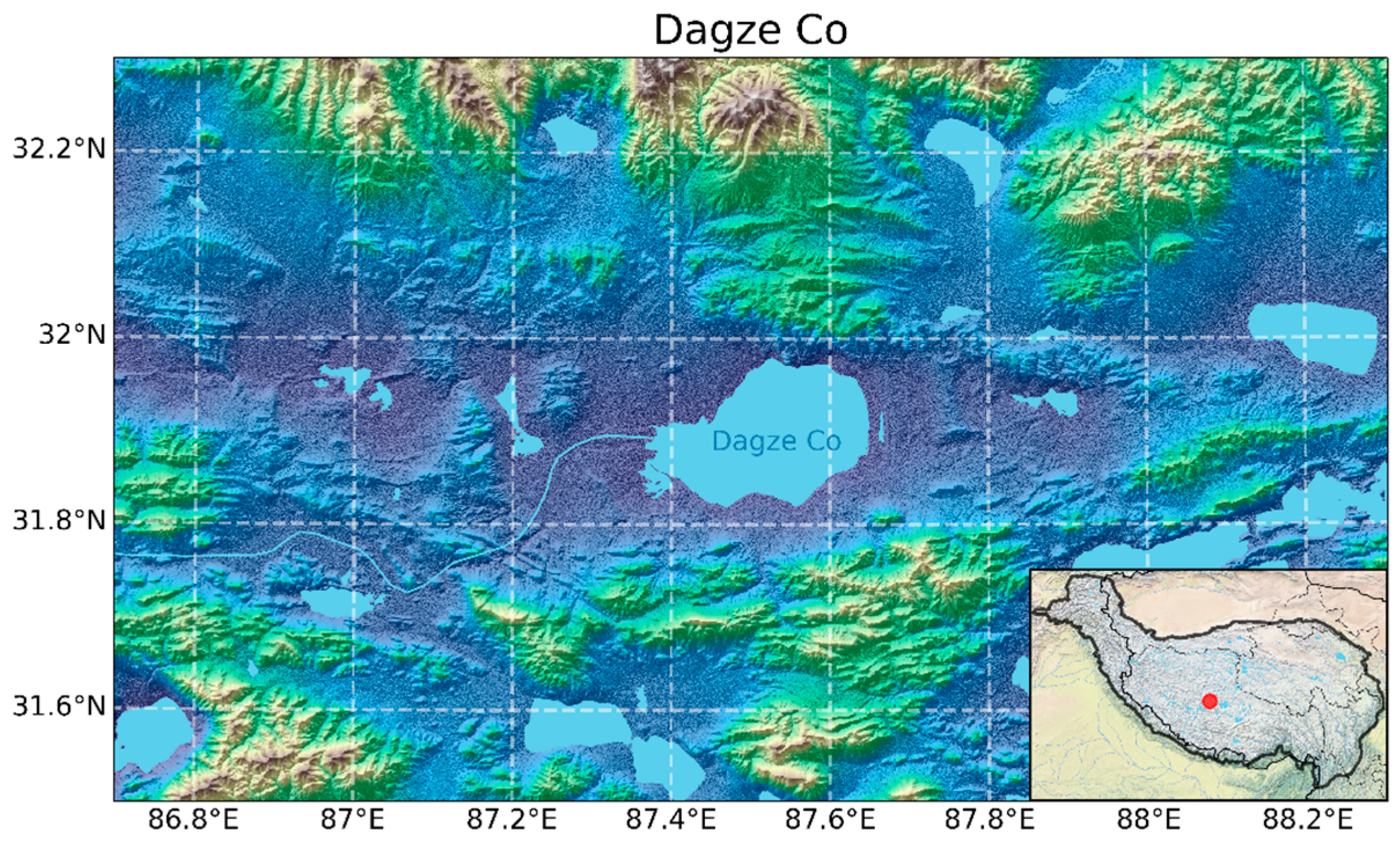
2.1. Study Area

Dagze Co (31°49′–31°59′ N, 87°25′–87°39′ E, 4450 m a.m.s.l.) is a brackish lake located in the central TP (Figure 1). The lake has a surface area of 245 km2, which is mainly fed by precipitation and the Bogcarg Zangbo River. The maximum depth of the lake is 38 m, roughly divided into several layers in terms of salinity: a layer from the lake surface to approximately 24 m with a slowly increasing salinity from 14.7 g L−1 to about 16.4 g L−1, a halocline at 25–29 m with a rapidly increasing salinity from 16.4 g L−1 to about 21 g L−1, and a layer with almost unchanged salinity of 21.4 g L−1 from 30 m to the bottom of the lake [54]. The thermocline appears at a depth of 16–23 m in summer (observed on 18 August 2012), while the ice-covered period lasts from November to April. The mean annual precipitation and air temperature observed by XainZa Meteorological Station, which is 150 km southeast of the lake, were 316 mm and 0.55 °C, respectively [55]. A multiyear averaged air pressure of 553 hPa and wind speed of 4.9 m s−1 were obtained by Shuanghu station 180 km away in the northeast direction of the lake.

2.2. Datasets

2.2.1. GloboLakes Surface Water Temperature

The Global Observatory of Lake Responses to Environmental Changes (GloboLakes) data product v4.0 was employed in this study to verify the simulated lake surface water temperature (LSWT). The GloboLakes provides daily values of LSWT for 2000 lakes globally distributed from 1995 to 2019 with a horizontal spatial resolution of 0.05° × 0.05°. The temperatures were retrieved from different orbit instruments, including the Along Track Scanning Radiometer (ATSR), Advanced Very High Resolution Radiometer (AVHRR), Moderate Resolution Imaging Spectroradiometer (MODIS), and Sea and Land Surface Temperature Radiometer (SLSTR), with the same algorithm and harmonized between sensors using overlap periods to ensure consistency [56]. The data represent the current state-of-the-art for LSWT record production and perform well in comparison with in situ measurements [57].

2.2.2. Dagze Co Water Temperature Monitoring Data

The Dagze Co water temperature monitoring data were used to validate the simulated water temperature in the deep layers of Dagze Co. The temperature loggers (HOBO Water Temperature Pro V2 Data Logger-U22-001, Onset Computer Corporation, 470 MacArthur Blvd, Bourne, MA, USA) were installed at 31°51′40.30″ N, 87°33′30.62″ E with a water depth of 37.3 m. There were 18 temperature loggers deployed along the water column, with 1-m intervals above 11 m depth, 2-m intervals from 11 to 23 m, and 3-m intervals below 23 m. The loggers commenced operation at 00:00 on 19 August 2012 and were retrieved on 20 August 2013, during which the water temperature was recorded at one-hourly intervals. The uppermost logger was placed at a ~4-m depth to prevent the influence of ice freezing and melting [54].

2.2.3. In situ Water Clarity Dataset

The water clarity data of Dagze Co was extracted from the in situ water quality parameters of the lakes on the Tibetan Plateau (2009–2020), which provides the in situ lake water parameters of 124 lakes in the TP [58]. These in situ parameters include water temperature, salinity, pH, chlorophyll-a concentration, blue-green algae concentration, turbidity, dissolved oxygen, fluorescent dissolved organic matter, and water clarity measured by Secchi Disk Depth (SDD).

2.2.4. China Meteorological Forcing Dataset (CMFD)

The forcing data of FLake were extracted from the China Meteorological Forcing Dataset (CMFD), which is a high spatial-temporal resolution gridded meteorological dataset for land surface processes simulation in China. The dataset is derived from a fusion of remote sensing products (GEWEX-SRB and TRMM), a reanalysis dataset (Princeton and GLDAS), and CMA in situ observation data, and provides 7 near-surface meteorological elements, including surface pressure, 2 m air temperature and specific humidity, 10 m wind speed, downward shortwave radiation, downward longwave radiation and precipitation rate with a temporal resolution of 3 h, and a spatial resolution of 0.1° from 1979 (currently up to 2018) [59]. It has become one of the most widely used datasets in China due to its better accuracy than the internationally available reanalysis data [18,50,52].

2.3. Model Description and Experimental Design

2.3.1. FLake Description and Configuration

FLake is a one-dimensional (1D) lake model capable of predicting the vertical temperature and mixing conditions in lakes of various depths on time scales from a few hours to many years [45,60]. FLake separates the water column into two layers, an upper mixed layer and an underlying thermocline layer, to parametrically represent the evolving temperature profile. The water temperature in the upper mixed layer is assumed to be vertically uniform. The thermocline layer between the upper mixed layer and the lake bottom is described based on the concept of self-similarity of the temperature-depth curve. The temperature profile of the thermocline can be fairly accurately parameterized through the following function of dimensionless depth:
θ s t θ z ,   t Δ θ t = Φ θ ζ       h t z h t + Δ h t
where t is time (s), z is the depth (m), θ s t is the upper mixed layer water temperature (K), h t is the mixed layer depth, Δ θ t = θ s t θ b t is the temperature difference across the thermocline of depth Δ h t , and θ b t is the temperature at the bottom of the thermocline. Φ θ ζ is a dimensionless “universal” function of the relative depth ζ = z h t / Δ h t , which satisfies two boundary conditions, Φ θ 0 = 0 and Φ θ 1 = 1 . It follows that the two-layer parameterization of the vertical temperature profile at time t is given by:
θ t =   θ s t                                             0 z h t θ s t θ s t θ b t Φ θ ζ           h t z h t + Δ h t
where the dimensionless shape function Φ θ ζ is calculated by:
Φ θ ζ = 40 3 C θ 20 3 ζ + 18 30 C θ ζ 2 + 20 C θ 12 ζ 3 + 5 3 10 3 C θ ζ 4
where C θ is the shape factor and can be computed by:
d C θ d t = sign d h t d t C θ m a x C θ m i n t r c C θ m i n       C θ m i n C θ C θ m a x
where t r c is the relaxation time scale (s), which indicates the time of the temperature profile in the thermocline evolving from one curve to the other, following the change of the sign in d h t d t . The minimum and maximum values of the shape factor are empirically set to C θ m i n = 0.5 and C θ m a x = 0.8 . The concept described above is also applied to describe the thermal structure of one ice layer, one snow layer on the lake ice, and two thermally active layers of lake sediments, which are included in the FLake.
The ice albedo in FLake is assumed to be represented by an empirical formulation based on the surface temperature:
α i c e = α m a x α m a x α m i n e x p 95.6 T f T s T f
where α m a x is the albedo of white ice (set to 0.6 by default), α m i n is the albedo of blue ice (set to 0.1 by default), T f is the freezing temperature (K), and T s is the ice surface temperature (K). The solar radiation transfers in water and ice/snow are described by a one-band exponential approximation of the Beer-Lambert decay law, for which an extinction coefficient of 3 m−1 in water and 1.0 × 10⁻⁷ in ice/snow is used in the default setting. Lake momentum fluxes, sensible heat fluxes, and latent heat fluxes were estimated using a parametric scheme that integrates the relationships between roughness length, potential temperature, specific humidity, and wind speed.
The function used to calculate friction velocity is:
u z u s = u * k ln z z 0 u + Ψ u ζ
where u z is the wind velocity at height z , u s is the wind velocity at the lake surface, u * is the friction velocity, k is the von Karman constant, z 0 u is roughness length of wind velocity, and Ψ u is Monin-Obukhov dimensionless functions in the similarity theory.
FLake intends to be coupled to different numerical weather prediction models (NWPs) and regional climate models (RCMs) as a lake parameterization scheme [23,28,61,62], but it can also be used as a stand-alone lake model. FLake has been well-tested by many studies worldwide, including a few lakes in the TP, and showed comparable or even better performance to many other 1D lake models in reproducing lake water temperature [39,43,46,63]. The simple two-layer stratification gives FLake the prominent merits of being computationally efficient and a small number of parameters have to be specified [18], but also limits its performance for lakes deeper than 50 m due to the absence of the hypolimnion layer between the thermocline and the lake bottom in deep lakes. However, this fact will not have much impact in our case as the water depth of Dagze Co is less than 50 m.

2.3.2. Experimental Design

The FLake model was driven by CMFD from 20 April 1990 to 31 December 2018 with a time step of 10 min. The running from 1990 to 1994 was for spin-up, while the result from 1995 to 2018 was used for analysis to avoid uncertainty of results in a single year. The simulation started on the ice-off date to simplify the initial condition. The lake depth of Dagze Co, which is one of the few parameters that need to be specified in FLake, was set to 37 m, equal to the water depth at the temperature profile monitoring site.
To evaluate the performance of the FLake model with different parameter settings in reproducing the LSWT and thermal structure of Dagze Co, a control experiment (CTRL, Table 1) with the default model configuration was first carried out. In the CTRL experiment, the extinction coefficient is set to 3 m−1, the friction velocity was calculated by Equation (6), and the ice-albedo was obtained from Equation (5).
In addition to the CTRL experiment, a series of sensitive experiments (SenExps in Table 1) were conducted by tuning some key parameters, i.e., extinction coefficient (Kd), friction velocity (u*), and ice albedo ( α i c e ), to explore the sensitivity of simulated water temperature to these key parameters. The extinction coefficient (Kd), which indicates the attenuation of solar radiation within the water column, is one of the most important parameters in controlling the water temperature profile. To investigate how the Kd affects water temperature, we performed a series of sensitivity experiments (SenExp_Kd), gradually changing Kd from 0.15 to 0.5 with a 0.05 interval, and from 0.6 to 2.8 with a 0.2 interval. The friction velocity (u*) in FLake, according to a previous study, also has a significant impact on water temperature [64]. Hence, experiments (SenExp_u*) with u* multiplied by a series of scale factors (varies from 1.2 to 2.0 with a 0.2 interval) were conducted to analyze the sensitivity of water temperature to u*. Previous studies have shown that the white ice albedo ( α m a x ) is a key parameter that determines lake ice phenology [65,66]. Thus, a series of sensitive experiments with changed white ice albedo (from 0.2 to 0.6 with a 0.05 interval) were conducted to explore its influence on ice phenology and water temperature.
To further improve the performance of FLake, three experiments were conducted by gradually optimizing each parameter mentioned above (OptExps in Table 1). According to previous studies, the Kd is closely correlated with water clarity (SDD) and can be approximated by the empirical equation [67]:
K d = 1.64 × S D D 0.76
The Kd in the CTRL experiment (3 m−1, corresponding to ~0.5 m SDD) seems too high for Dagze Co, which has a mean in situ SDD of ~7 m. Hence, the Kd was tuned to ~0.37 m−1 according to Equation (7) in the parameter optimization experiments (OptExp_1). Then, the friction velocity was also tuned by multiplying an optimized scale factor to minimize the deviation of the simulated LSWT (OptExp_2). Based on the sensitive experiments, the white ice albedo ( α m a x ) in FLake has generally been overestimated by many lake models before in TP lakes, which are barely covered by any snow in winter, and was also tuned to an optimized value to further minimize the deviation of the reproduced LSWT. The tuning process of these parameters was both efficient and physically reasonable for the representation of lake properties. In addition to the above parameter tuning process, a salinity parameterization scheme was added to FLake to consider the effect of salinity (S) on the maximum density temperature ( T m ) and water freezing point ( T f ). The equations are as follows [68]:
T m ° C = 3.98 0.216 S
T f ° C = 0.055 S
where S is the salinity (g L−1) of the lake water.

2.4. Methodology

The statistics including the mean bias error (BIAS), correlation (R), and root-mean-square-error (RMSE) are adopted to evaluate and improve the model performance. The formulas for these statistics are shown as follows:
B I A S = 1 N i = 1 N S i O i
R M S E = 1 N i = 1 N S i O i 2
R = i = 1 N S i S ¯ O i O ¯ i = 1 N S i S ¯ 2 i = 1 N O i O ¯ 2
where N is the number of points (in time or space). S i ( O i ) is the simulation (observation) at point i , and S ¯ ( O ¯ ) is the mean value of the simulation (observation) over N sample points. Both lower BIAS and RMSE suggest a better performance of the simulation, while higher R indicates a larger similarity in the temporal variation between the simulation and observation.

3. Results

3.1. Validation of Default FLake Simulations

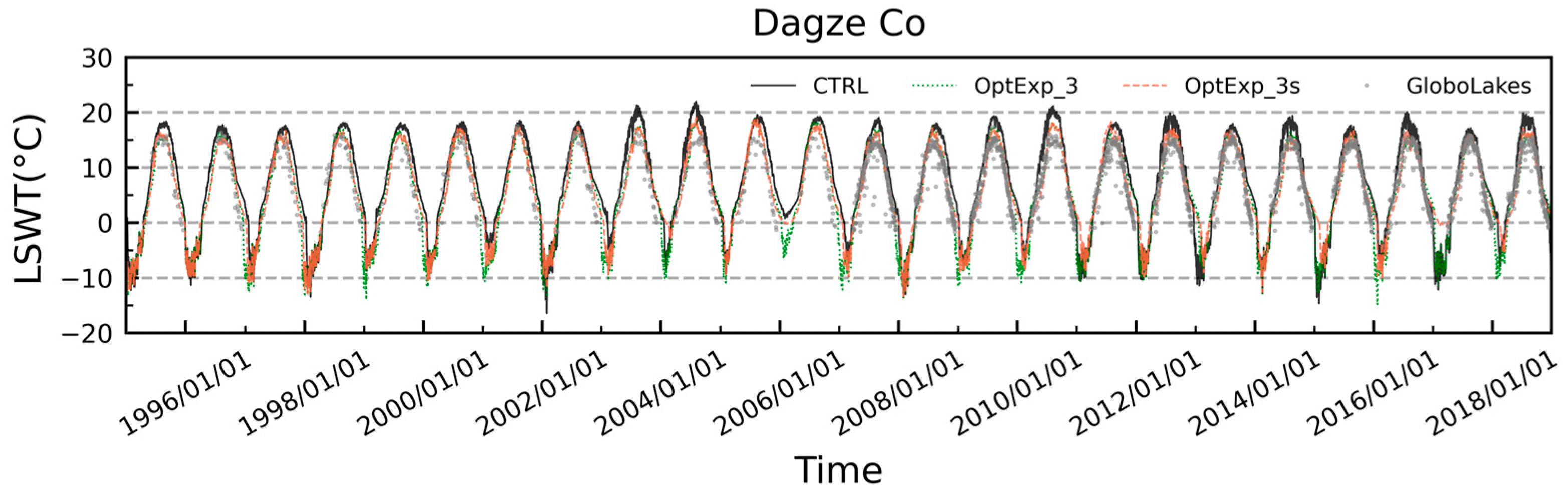
3.1.1. Lake Surface Water Temperature

To reveal the ability of the FLake model to simulate the structure of the Dagze Co with default parameter settings, we first compare the LSWT from the CTRL experiment with the observation. In the same way as observations [54], the CTRL experiment shows that Dagze Co is frozen from late November or early December to April each year. During the ice-covered period, the simulated lake surface temperature sharply fluctuates because the lake surface is frozen, which reduces the specific heat capacity of the lake surface and blocks the heat exchange with the deep lake water, so the lake surface temperature is greatly influenced by the air temperature. Figure 2 exhibits that although the seasonal variation of LSWT and ice on/off characteristics of Dagcze Co can be roughly simulated by FLake, there is still a significant deviation between simulation and observation. In particular, the LSWT is underestimated in winter (December-February) with a large systematic negative bias, which may be caused by an overestimation of FLake in lake ice albedo for alpine lakes on the TP [69]. While the LSWT is generally overestimated in summer (June–August) with a large systematic positive bias.

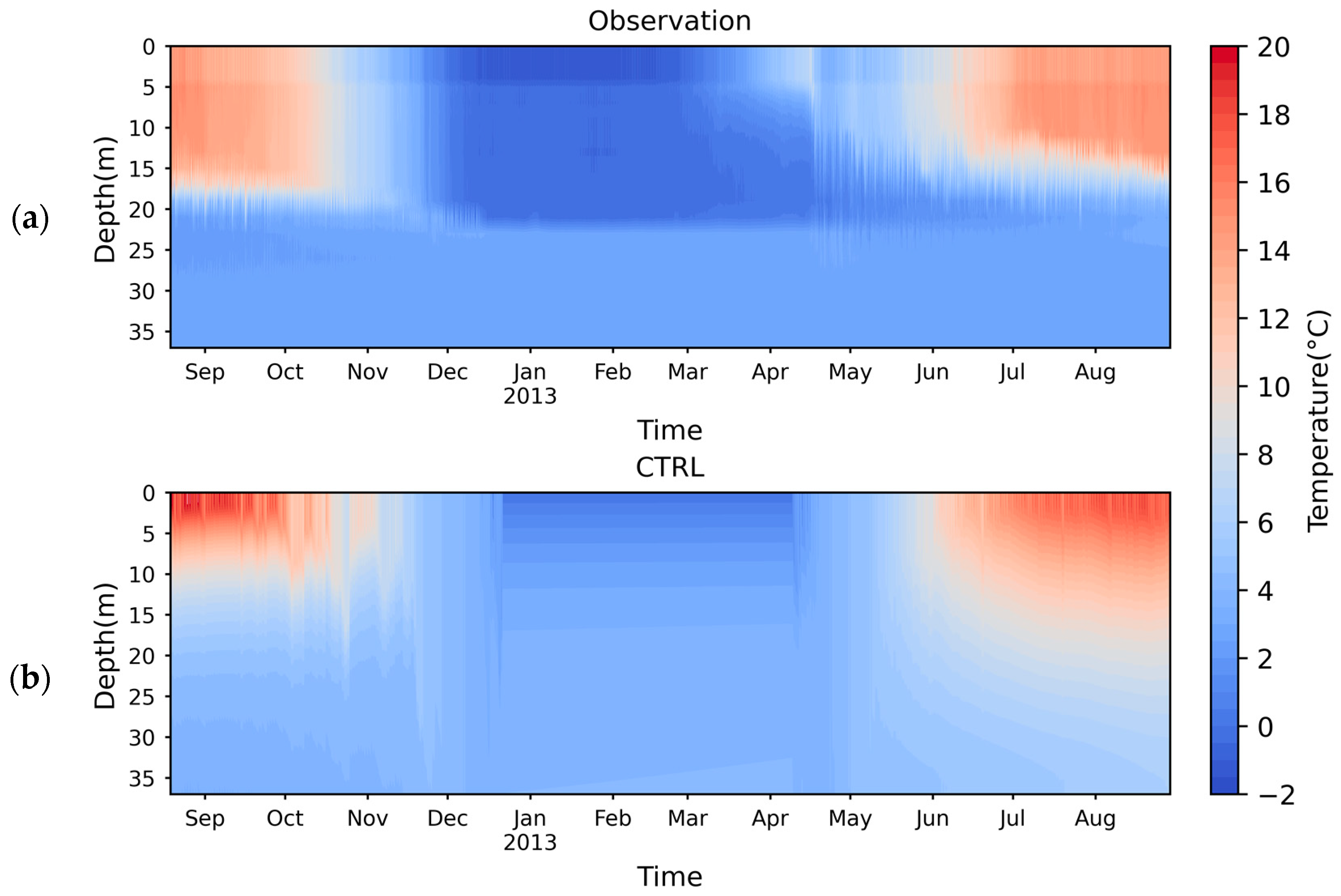
3.1.2. Vertical Temperature Profile

In Figure 3, the time-depth distribution of the daily water temperature of the Dagze Co from observation and simulation is shown. According to the observation (Figure 3a), the water temperature during the ice-covered period (December–April) is generally under 2 °C in the upper layer of the lake (depth of 0–20 m), and gradually increases to ~4 °C at the bottom of the lake, except that after March the water temperature near the surface gradually increased to ~4–7 °C. However, after the ice break-up, the temperature near the surface layer suddenly dropped to 2–3 °C during a short period in late April and then began to increase from May to August. The temperature in the epilimnion of the lake eventually exceeded 10 °C in August, while the temperature in the hypolimnion below 20 m was essentially maintained at about 4 °C.
Figure 3b shows the overall vertical thermal structure of the lake reproduced by the FLake in the CTRL experiment. Compared to the observation, the simulated water temperature near the surface layer (about 0–5 m) during the ice-covered period is also lower than 2 °C, but there is a significant rise in temperature from 5–20 m, gradually increasing to 4 °C, as well as water temperature for the bottom layer of the lake. From June to early August, the temperature in the upper layer of the lake exceeded 10 °C, especially for the epilimnion with a temperature near 20 °C. An obvious temperature gradient appears in metalimnion with a depth ranging from 5 m to 20 m, where the water temperature dropped to about 8 °C. For the hypolimnion with a depth of 20–37 m, the water temperatures were higher compared to the observation.
In conclusion, the FLake model with default parameter settings can reproduce the overall structure of the observed water temperature, with a relatively smaller vertical temperature gradient during the ice-covered period and larger vertical temperature gradients during the stratified season. However, there are still obvious deviations in the simulation compared to the observation. FLake produced a shorter ice-covered period, mainly due to a later ice-on date and an earlier ice-off date. Additionally, the water temperature in the mixed layer during the stratified season was overestimated, with a relatively shallower mixed layer depth from September to October 2012.

3.2. Parameter Sensitivity Experiment

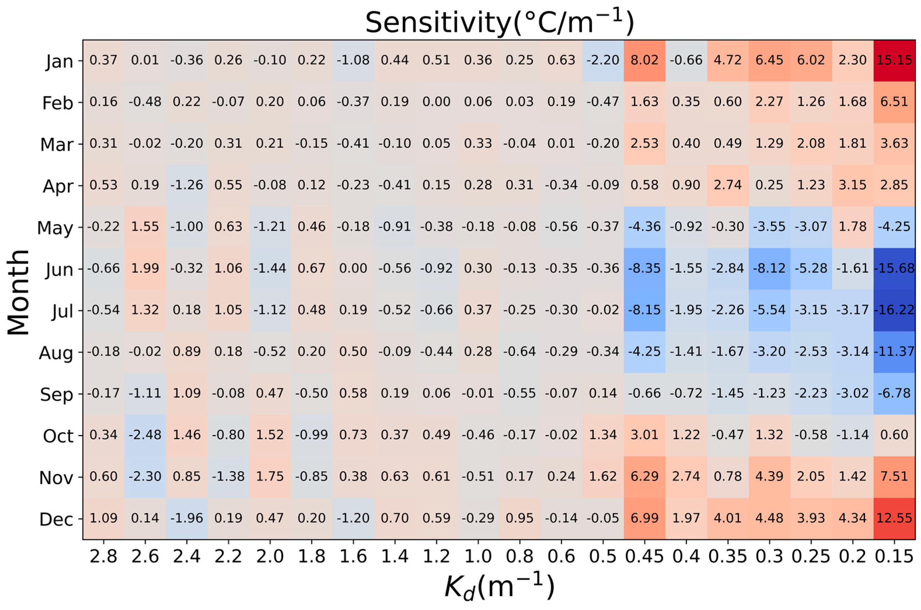
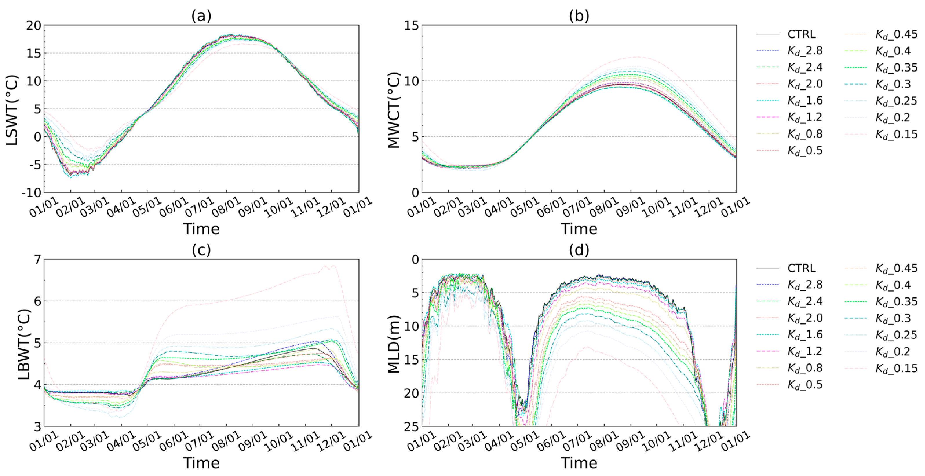
3.2.1. Extinction Coefficient

To improve the applicability of the FLake model in Dagze Co, it is necessary to systematically investigate the sensitivity of some key parameters in the FLake on lake thermal features first. By setting the water extinction coefficient (Kd) of Dagze Co to different values, the changes in simulated water temperature for both the surface and interior of the lake with different transparency conditions were investigated. According to the observation, the Secchi Disk Depth (SDD) for Dagze Co is ~7 m, corresponding to a Kd of ~0.37 m−1, which is much smaller than the default value of 3 m−1 in FLake. Therefore, the extinction coefficient was gradually changed from 2.8 m−1 to 0.6 m−1 with an interval of 0.2 m−1, and from 0.5 m−1 to 0.15 m−1 with an interval of 0.05 m−1. As shown in Figure 4 (only some of the results are shown), the curves of LSWT, mean water column temperature (MWCT), lake bottom water temperature (LBWT), and mixed layer depth (MLD) apparently changed with the extinction coefficient. For turbid lake water with larger Kd, solar radiation is absorbed by the particles in the water, leading to a small depth penetrated by solar radiation. Thus, the heating of solar radiation mainly operates in a shallow layer of the lake. As shown in Figure 4, larger Kd corresponds to a warmer LSWT, colder LBWT, and smaller MLD, while lower Kd produces the opposite result. The higher LSWT of the turbid lake leads to an increase in the latent and sensible heat fluxes at the lake surface with accelerated heat exchange between the lake and the atmosphere, which makes the LSWT respond more quickly to the solar radiation and air temperature. This explains the fluctuations in the LSWT with higher Kd and smoother LSWT with lower Kd, as well as the fact that the LSWT of the higher Kd is warmer in the spring and colder in the autumn, as well as lower MWCT, which is just the opposite for the result with small Kd.
Figure 5 illustrates the sensitivity of LSWT to Kd, representing the variation in LSWT corresponding to a 1 m−1 change in Kd. Generally, LSWT is not very sensitive to changes in Kd when the Kd is greater than 0.5 m−1, and there is no evident correlation between changes in LSWT and Kd. However, once Kd is less than 0.5 m−1, LSWT becomes quite sensitive to changes in Kd with pretty obvious patterns between the two of them. That is, LSWT generally decreases with decreasing Kd from May to September, while increases with decreasing Kd from October to April occur in the following year. With a decreasing Kd, the most pronounced cooling in LSWT occurred in June and July, especially when the Kd is equal to 0.15, in which case each 1 m−1 reduction in Kd will result in a maximum decrease of 16.22 °C for LSWT. In contrast, LSWT increased the most in January and December as Kd reduced, which also reaches the maximum value of 15.15 °C when Kd is equal to 0.15 m−1.

3.2.2. Friction Velocity
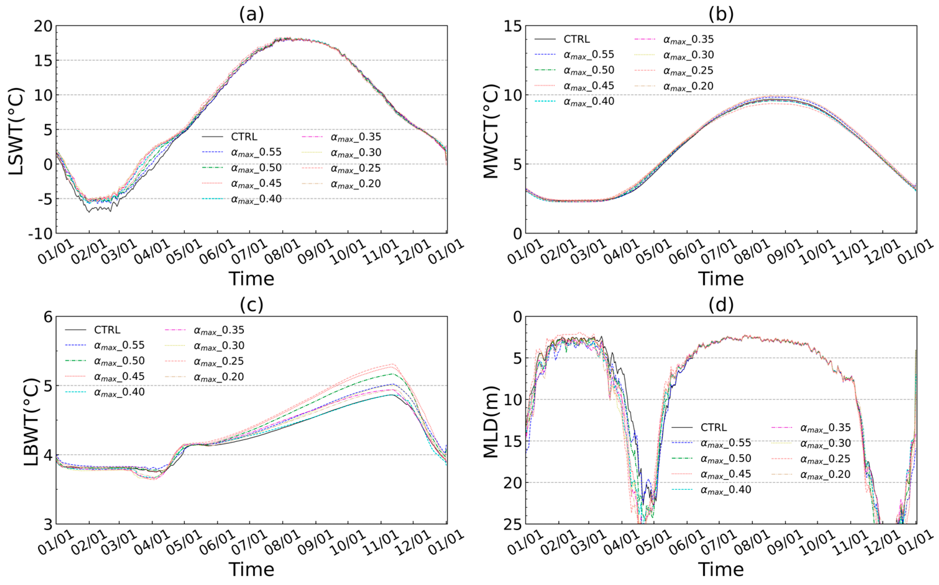
A recent study in Ngoring Lake found that the friction velocity is underestimated by the FLake compared to the observed value, resulting in a significant positive deviation in LSWT produced by FLake [64]. Hence, a series of sensitivity experiments with the friction velocity u* increased by a factor of 1.2, 1.4, 1.6, 1.8, and 2 were conducted to investigate the influence of different friction velocities on the simulated LSWT in Dagze Co. As Figure 6 shows, compared with the CTRL experiment with default parameter setting, the simulated LSWT, MWCT, LBWT, and MLD apparently changed with different friction velocities. As the friction velocity increases, LSWT generally decreases and fluctuates more dramatically. The ice-on date is advanced while the ice-off date is delayed, resulting in a longer ice-covered period. The effect of friction velocity on lake thermal structure is not as pronounced as Kd, but still considerable. In addition to a decrease in the LSWT, the MWCT of the lake also slightly decreased with increasing friction velocity (Figure 6b). Although the LSWT and MWCT decreased, there was no significant change in the LBWT (Figure 6c). Variation in the MLD demonstrated that the larger the friction velocity, the deeper the MLD, as well as more obvious fluctuations. The reason for the decrease in LSWT and MCWT is that the increase in friction velocity increases the air-lake heat exchange and vertical mixing of the lake.

3.2.3. Ice Albedo

The lake ice albedo can affect the amount of solar radiation absorbed by the ice during the ice-covered period of the lake, further affecting the ice-off date. The climate on TP is dry and with strong solar radiation in winter, resulting in sparse snow over the lake ice and thus a generally lower lake surface albedo compared to low-lying regions. Observations indicate that the actual ice albedo for lakes on the TP is much smaller than the value used in the lake models [66]. Therefore, to verify the effect of the ice albedo on simulated lake thermal conditions, the white ice albedo in FLake is gradually reduced from the default value of 0.6 to 0.2 with an interval of 0.05. As shown in Figure 7, during the ice-covered period, LSWT slightly increases with the decrease of lake ice albedo, while the variation is not obvious in other months. As the ice albedo decreases, the simulated ice-covered period generally shortens, as well as an increase in LSWT just before ice-on and after ice-off. This is because the smaller the ice albedo is, the more solar radiation the ice absorbs, and thus the faster the ice melts. Lake ice can prevent solar radiation from penetrating the lake water, and an early ice-off will lead to more absorbed solar radiation and rapidly rising LSWT after the ice-off. The absorbed energy will be stored in the lake and released until the cooling stage of the lake. In such a case, the lake will maintain a higher temperature before the ice-on, resulting in a delayed ice-on date. Therefore, the lake ice albedo can not only affect the duration of the ice-covered period but also the LSWT before and after the ice-covered period. The ice albedo can also affect the internal thermal feature of the lake, the MWCT slightly increases from July to November as the ice albedo decreases, but not significantly in other months. The change in albedo has no obvious effect on LBWT, which slightly increases from June to December with a decrease in albedo. The MLD generally shows a slightly deepening trend, especially in the turnover period. In general, the decrease in ice albedo not only affects the ice-covered duration of the lake but also indirectly affects the solar radiation absorbed by the lake and the lake-air energy exchange, further affecting the surface and internal thermal features of the lake.

3.3. Improvements in FLake Performance

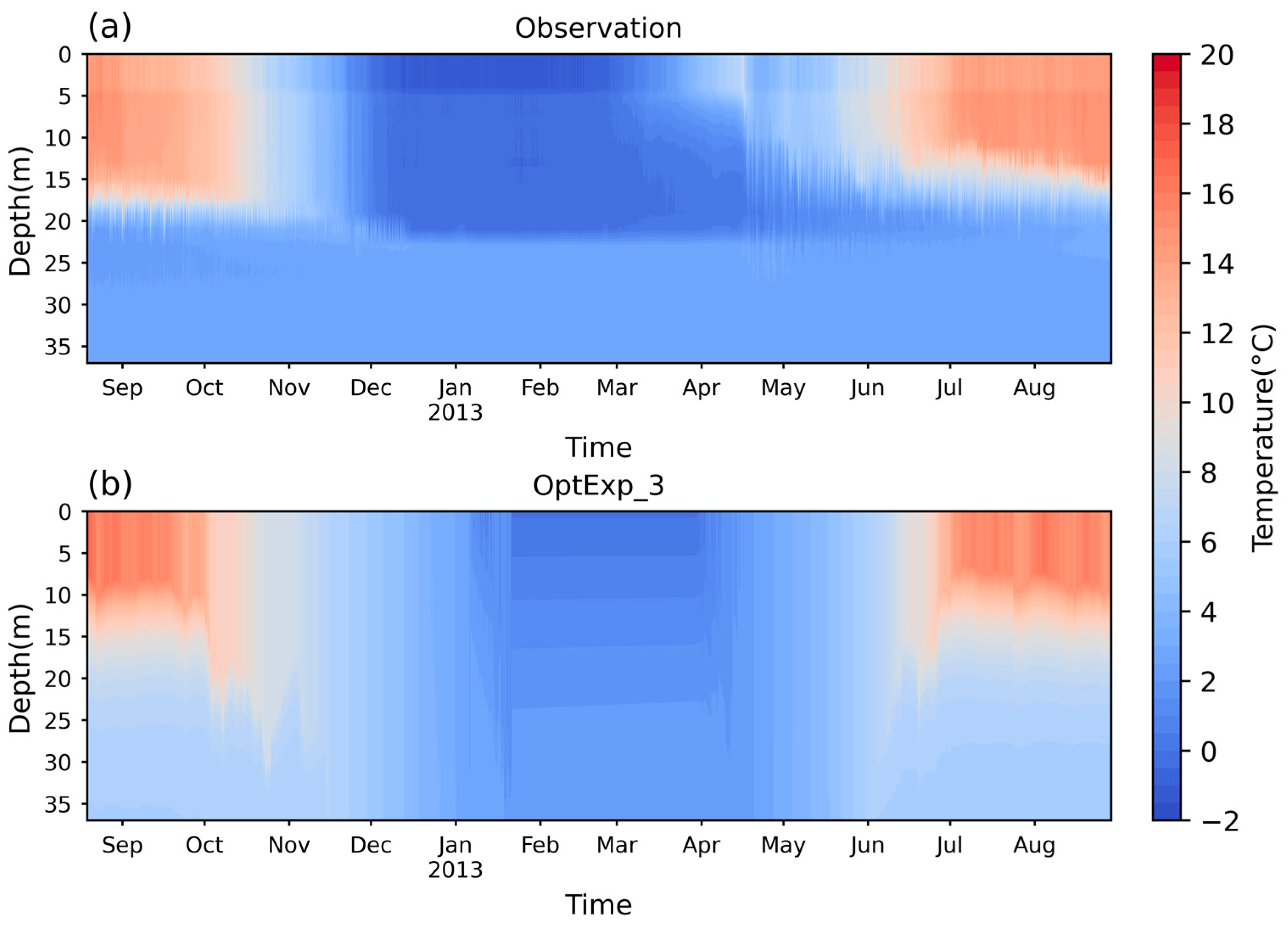
3.3.1. Optimization of Key Parameters

Based on the previous studies and results from sensitive experiments conducted above, three sets of experiments with optimized parameters were conducted to gradually improve the performance of the FLake model for Dagze Co (OptExp in Table 1). The CTRL experiment with default parameters settings was used as a reference. In the OptExp_1 experiment, the Kd was modified from 3.0 m−1 to 0.37 m−1, which is calculated by Equation (7) with an SDD of ~7 m in Dagze Co. In addition to optimized Kd, the OptExp_2 experiment enlarged the friction velocity (u*) with a factor of 2. In the OptExp_3 experiment, the white ice albedo was further changed from 0.6 to 0.25. Through the above experiments, three key parameters were gradually optimized to enhance the performance of the FLake model.
Figure 8 shows the LSWT of Dagze Co from GloboLakes observation and FLake simulation in different experiments with optimized parameters. In the CTRL experiment, the FLake overestimated LSWT in summer and autumn, and the lake warmed more rapidly in spring and also cooled more rapidly in autumn compared to observation. After the Kd was changed to 0.35 m−1 in the OptExp_1, although the overestimation of LSWT still exists, the seasonal variation in LSWT was more consistent with observations. In the OptExp_2, with friction velocity enlarged by a factor of 2, the overestimation of LSWT in summer and autumn was significantly reduced, but the ice-off date is still later than the observation. Hence, based on the above experiments, the white ice albedo in FLake was further changed to 0.25, resulting in a significant improvement in the LSWT simulation compared to the observation.
As the statistics results show in Table 2, compared with observations, the CTRL experiment has a bias of 3.08 °C, an RMSE of 3.62 °C, and a correlation coefficient of 0.91. After changing the Kd in OptExp_1, although the bias, RMSE, and correlation coefficient of simulated LSWT have almost not been reduced or are even slightly worse, the phase of annual variation of LSWT is more consistent with observation. With the friction velocity tuned, the bias and RMSE are significantly reduced to 2.20 °C and 2.72 °C, with a correlation coefficient of 0.86. In OptExp_3, following optimized Kd and friction velocity, the white ice albedo was also modified to 0.25, the bias and RMSE of LSWT further reduced to 2.00 °C and 2.48 °C, respectively, while the correlation coefficient was re-raised to 0.90. This result indicates that the capability of FLake in reproducing the LSWT of Dagze Co was substantially improved by the optimization of key parameters.
In addition to an improvement in the LSWT simulation, the optimization of the three key parameters also enhances the capability of FLake to reproduce the internal thermal structure of the lake. As Figure 9 shows, compared with the CTRL experiment (shown in Figure 3), the OptExp_3 experiment produced a warmer metalimnion and increased MLD, mainly due to a significant increase in absorbed solar radiation for water in the metalimnion by reducing the Kd. Meanwhile, the overestimated MLWT in the epilimnion of the lake by the CTRL experiment was also decreased in the OptExp_3 experiment, which ascribed to a reduced Kd as well as increased friction velocity that accelerated the release of heat flux from the lake into the atmosphere. In addition, the lake ice melted earlier in the OptExp_2 experiment compared to the CTRL experiment due to the reduction in ice albedo, leading to more absorption of solar radiation after ice-off, which increased the LBWT as well as delaying the ice-on date. With the optimized key parameters, the simulation result by OptExp_3 is closer to the observations, indicating the performance of FLake in reproducing the thermal structure of Dagze Co has been significantly improved.

3.3.2. Salinity Parameterization

As a saline lake, the salinity in Dagze Co can affect its freezing temperature as well as its maximum density temperature, which exerts an influence on the mixing regime, and thus, the thermal structure of the lake. However, the original FLake does not consider the influence of salinity. To investigate the influence of salinity on the thermal features of Dagze Co, a simplified salinity parameterization scheme (Equations (8) and (9)) was integrated into FLake in addition to the optimization of three key parameters. As shown in Figure 9, compared to the original FLake simulation results, the OptExp_3 experiment greatly improved the accuracy of simulated LSWT by optimizing Kd, friction velocity, and ice albedo in FLake. As shown in Figure 10, with the integration of the salinity parameterization scheme, the simulated LSWT during the open-water period shows no significant change, but the ice duration period and LSWT before and after the ice duration period slightly change. The ice-on date was slightly delayed, while the ice-off date was slightly advanced, which is closer to the observation. The bias, RMSE, and correlation coefficient of LSWT produced by the OptExp_3s experiment were further enhanced from 2.0 °C, 2.48 °C, and 0.9 to 1.84 °C, 2.28 °C, and 0.91, respectively.

4. Discussion

In CTRL experiments, FLake with default parameter settings slightly underestimated the LSWT of Dagze Co in spring and winter, while significantly overestimated the LSWT in summer and autumn. The same conclusion was reached in another study after modeling 94 lakes larger than 100 km2 in China using FLake [47]. Additionally, simulations in Qinghai Lake, the largest lake on the TP, also show an overestimation of LSWT by FLake in summer and autumn [50], demonstrating the commonality of this distinguishing feature of FLake. However, a significant difference appears between our study and the previous studies in the simulation of the ice-covered period. Compared to the previous simulations in Qinghai Lake, which generally produced delayed both ice-on and ice-off data [50], the CTRL simulation in this study produced a delayed ice-on date, but with an earlier ice-off date.
The extinction coefficients strongly affect the LSWT and vertical thermal structure during summer. Previous studies have tried tuning Kd to improve the performance of FLake and achieved promising outcomes [39,47]. In the sensitive experiments, we further analyzed the sensitivity of LSWT to varying Kd in different months, revealing an abrupt increase in sensitivity of LSWT to Kd when it is less than 0.5 m−1, as well as the inverse response of LSWT to Kd between the warm and cold seasons. However, the sensitivity of LSWT to Kd is still nonlinear when Kd is less than 0.5 m−1, indicating that there may be other factors exerting an influence on the sensitivity of LSWT to Kd. This result is consistent with the findings in previous studies, which suggest that the response of LSWT to change in Kd is nonlinear, and is more sensitive when the Kd is less than 0.5 m−1 [70,71]. Therefore, it is quite reasonable for lake models to set the default Kd to 3 m−1 since Kd for most of the lakes in low-lying areas is greater than 0.5 m−1. However, most of the lakes over TP are oligotrophic with fewer biochemical processes and higher clarity, resulting in a Kd smaller than 0.5 m−1 [72]. In such a case, the LSWT will be very sensitive to changes in Kd for lakes over TP, indicating the importance of optimizing Kd before applying FLake to TP lakes. In previous studies, different parameters, e.g., Kd, depth, water albedo, ice albedo, and temperature of maximum water density, have been optimized to improve the performance of FLake, while few studies have concerned the friction velocity [39]. Our studies demonstrated that the friction velocity can significantly influence the LSWT and thermal structure of the lake. By increasing the friction velocity in FLake, the positive deviation of LSWT produced by FLake in the summer was significantly reduced. In line with previous studies, the SenExp_ α experiments in our study indicate that ice albedo is the main lake parameter that affects the ice-off date [47]. The overestimation of ice albedo in FLake means more solar radiation will be reflected by the lake, which affects the melting of lake ice and leads to a delay in the ice-off date. Compared to previous studies, the SenExp_ α experiments in our study further demonstrated that the ice-albedo also can affect the LSWT before and after the ice-covered period and even the internal thermal structure of the lake. Compared to the previous study in Nam Co, which set the temperature of maximum water density to an empirical value [39], another important contribution of this study is the adoption of a simple salinity parameterization that considers the effect of salinity on the temperature of maximum water density and the freezing point, which further enhanced the ability of FLake in reproducing the ice-duration period.

5. Conclusions

In this study, forced by the CMFD dataset, the suitability of applying the 1D lake model FLake in Dagze Co on the central TP was investigated based on a one-year in situ vertical temperature observation in Dagze Co. Then, a series of sensitive experiments were conducted to reveal the influence of three key parameters of FLake on lake thermal features. According to the physical characteristics and sensitive experiments, these key parameters were optimized to improve the performance of FLake. The main conclusions are as follows.
FLake with default settings exhibits significant deviations in simulating the LSWT and thermal profile of Dagze Co. The LSWT is overestimated, mainly in summer and autumn, with a bias and RMSE of 3.08 °C and 3.62 °C. Meanwhile, the simulated warming of LSWT in spring and cooling of LSWT in autumn are both faster than the observation, and the MLD simulated by FLake is shallower than the observation.
The sensitive experiments on the Kd, friction velocity, and ice albedo revealed that FLake is very sensitive to these parameters. The reduction in Kd slows the warming and cooling rate of the LSWT during its rising and declining phases, respectively, as well as deepening MLD during the stratified period. The sensitivity of LSWT in Kd is nonlinear, which abruptly changes when Kd is less than 0.5 m−1. The increase in friction velocity will lead to an obvious decrease in LSWT, MCWT, and a slight increase in the MLD. Meanwhile, the reduction in ice albedo would cause an earlier ice-off date and a higher LSWT just after the ice-off, resulting in a slight warming of MWCT and LBWT during the following open water period.
The optimization of three key parameters in FLake significantly improved the performance of FLake. With Kd adjusted from 3.0 m−1 to 0.25 m−1, the variation patterns of simulated LSWT became more consistent with observation. The enlarged friction velocity substantially diminished the overestimation of LSWT produced by FLake in summer. Setting the white ice albedo from 0.60 to 0.25 increased the accuracy of FLake in modeling the ice duration period, especially the ice-off date. The experiments with salinity parameterization indicate that salinity has a minor effect on the LSWT during the open water period, while slightly affecting the ice duration period, which delays the ice-on date and advances the ice-off date, leading to a better approximation of the ice-cover simulation to that of observation. After the parameter optimization and salinity parameterization, the bias and RMSE of simulated LSWT reduced to 1.84 °C and 2.28 °C, respectively.
However, there are still limitations in this work. The primary one is the deviation originating from the forcing data, which is not calibrated in our study because of the scarcity of observations. Wind speed extracted from CMFD, which is mainly provided by land observation stations, may be significantly underestimated over the lake surface. In such a case, the optimized friction velocity may be different from the value used in this study. In addition, Kd was simply set to a constant value in this study, which is not realistic as Kd varies with water transparency. Hence, the parameterization scheme of Kd based on satellite-observed water transparency needs to be established in the future.

Author Contributions

Conceptualization, D.S. and L.W.; methodology, B.C.; software, M.L. (Minghua Liu); validation, Z.L. and X.S.; formal analysis, L.W.; investigation, J.L.; resources, L.W.; data curation, D.S.; writing—original draft preparation, B.C.; writing—review and editing, D.S. and M.L. (Minghua Liu); visualization, M.L. (Minghua Liu) and D.S.; supervision, D.S.; project administration, L.W.; funding acquisition, L.W. and M.L. (Maoshan Li). All authors have read and agreed to the published version of the manuscript.

Funding

This research was funded by the National Key Research and Development Program of China (2019YFE0197600), the National Natural Science Foundation of China (Grant Nos. 42275044, 42230610, 42305026), the CAS “Light of West China” program (Grant No. E129030101), the Scientific Research Foundation of Chengdu University of Information Technology (Grant No. KYTZ202126), and the Science and technology Research and Development Program of China National Railway Group (Grant No. P2021G047).

Data Availability Statement

The GloboLakes Surface Water Temperature Dataset can be downloaded freely from http://www.laketemp.net/home/, accessed on 1 July 2023. The Dagze Co water temperature monitoring data, In situ Water Clarity Dataset, and China Meteorological Forcing Dataset (CMFD) are all openly available from https://data.tpdc.ac.cn/, accessed on 1 July 2023.

Acknowledgments

We thank Mingda Wang for providing temperature observation data in Dagze Co, which can be openly accessed in the National Tibetan Plateau Third Pole Environment Data Center (https://data.tpdc.ac.cn/).

Conflicts of Interest

The authors declare no conflict of interest.

References

  1. Zhang, G.Q.; Luo, W.; Chen, W.F.; Zheng, G.X. A robust but variable lake expansion on the Tibetan Plateau. Sci. Bull. 2019, 64, 1306–1309. [Google Scholar] [CrossRef]
  2. Ma, R.H.; Yang, G.S.; Duan, H.T.; Jiang, J.H.; Wang, S.M.; Feng, X.Z.; Li, A.N.; Kong, F.X.; Xue, B.; Wu, J.L.; et al. China’s lakes at present: Number, area and spatial distribution. Sci. China Earth Sci. 2010, 54, 283–289. [Google Scholar] [CrossRef]
  3. Adrian, R.; O’Reilly, C.M.; Zagarese, H.; Baines, S.B.; Hessen, D.O.; Keller, W.; Livingstone, D.M.; Sommaruga, R.; Straile, D.; Donk, E.V. Lakes as sentinels of climate change. Limnol. Oceanogr. 2009, 54, 2283–2297. [Google Scholar]
  4. Sun, L.; Wang, B.; Ma, Y.; Shi, X.; Wang, Y. Analysis of ice phenology of middle and large lakes on the Tibetan Plateau. Sensors 2023, 23, 1661. [Google Scholar] [CrossRef] [PubMed]
  5. Shi, Y.; Huang, A.; Ma, W.; Wen, L.; Zhu, L.; Yang, X.; Wu, Y.; Gu, C. Drivers of warming in lake Nam Co on Tibetan Plateau over the past 40 years. J. Geophys. Res. Atmos. 2022, 127, e2021JD036320. [Google Scholar] [CrossRef]
  6. Liu, Y.; Chen, H. Future warming accelerates lake variations in the Tibetan Plateau. Int. J. Climatol. 2022, 42, 8687–8700. [Google Scholar] [CrossRef]
  7. Gilarranz, L.J.; Narwani, A.; Odermatt, D.; Siber, R.; Dakos, V. Regime shifts, trends, and variability of lake productivity at a global scale. Proc. Natl. Acad. Sci. USA 2022, 119, e2116413119. [Google Scholar] [CrossRef]
  8. Wang, B.; Ma, Y.; Wang, Y.; Lazhu; Wang, L.; Ma, W.; Su, B. Analysis of lake stratification and mixing and its influencing factors over high elevation large and small lakes on the Tibetan Plateau. Water 2023, 15, 2094. [Google Scholar] [CrossRef]
  9. Zhang, Y.B.; Shi, K.; Zhang, Y.L.; Moreno-Madrinan, M.J.; Xu, X.; Zhou, Y.Q.; Qin, B.Q.; Zhu, G.W.; Jeppesen, E. Water clarity response to climate warming and wetting of the Inner Mongolia-Xinjiang Plateau: A remote sensing approach. Sci. Total Environ. 2021, 796, 148916. [Google Scholar] [CrossRef]
  10. Brown, L.C.; Duguay, C.R. The response and role of ice cover in lake-climate interactions. Prog. Phys. Geogr. Earth Environ. 2010, 34, 671–704. [Google Scholar] [CrossRef]
  11. Woolway, R.I.; Sharma, S.; Weyhenmeyer, G.A.; Debolskiy, A.; Golub, M.; Mercado-Bettin, D.; Perroud, M.; Stepanenko, V.; Tan, Z.; Grant, L.; et al. Phenological shifts in lake stratification under climate change. Nat. Commun. 2021, 12, 2318. [Google Scholar] [CrossRef]
  12. Maberly, S.C.; O’Donnell, R.A.; Woolway, R.I.; Cutler, M.E.J.; Gong, M.; Jones, I.D.; Merchant, C.J.; Miller, C.A.; Politi, E.; Scott, E.M.; et al. Global lake thermal regions shift under climate change. Nat. Commun. 2020, 11, 1232. [Google Scholar] [CrossRef] [PubMed]
  13. Lu, P.; Cao, X.; Li, G.; Huang, W.; Leppäranta, M.; Arvola, L.; Huotari, J.; Li, Z. Mass and heat balance of a lake ice cover in the central Asian arid climate zone. Water 2020, 12, 2888. [Google Scholar] [CrossRef]
  14. Zhao, Z.; Huang, A.; Ma, W.; Wu, Y.; Wen, L.; Lazhu; Gu, C. Effects of lake Nam Co and surrounding terrain on extreme precipitation over Nam Co basin, Tibetan Plateau: A case study. J. Geophys. Res. Atmos. 2022, 127, e2021JD036190. [Google Scholar] [CrossRef]
  15. Su, D.S.; Wen, L.J.; Gao, X.Q.; Lepparanta, M.; Song, X.Y.; Shi, Q.Q.; Kirillin, G. Effects of the largest lake of the Tibetan Plateau on the regional climate. J. Geophys. Res.-Atmos. 2020, 125, e2020JD033396. [Google Scholar] [CrossRef]
  16. Wu, Y.; Huang, A.N.; Yang, B.; Dong, G.T.; Wen, L.J.; Lazhu; Zhang, Z.Q.; Fu, Z.P.; Zhu, X.Y.; Zhang, X.D.; et al. Numerical study on the climatic effect of the lake clusters over Tibetan Plateau in summer. Clim. Dyn. 2019, 53, 5215–5236. [Google Scholar] [CrossRef]
  17. Kirillin, G.; Wen, L.; Shatwell, T. Seasonal thermal regime and climatic trends in lakes of the Tibetan highlands. Hydrol. Earth Syst. Sci. 2017, 21, 1895–1909. [Google Scholar] [CrossRef]
  18. Lazhu; Yang, K.; Wang, J.B.; Lei, Y.B.; Chen, Y.Y.; Zhu, L.P.; Ding, B.H.; Qin, J. Quantifying evaporation and its decadal change for Lake Nam Co, central Tibetan Plateau. J. Geophys. Res.-Atmos. 2016, 121, 7578–7591. [Google Scholar] [CrossRef]
  19. Dombrovsky, L.A.; Kokhanovsky, A.A. Solar heating of ice-covered lake and ice melting. J. Quant. Spectrosc. Radiat. Transf. 2023, 294, 108391. [Google Scholar] [CrossRef]
  20. Boehrer, B.; Schultze, M. Stratification of lakes. Rev. Geophys. 2008, 46, e2006rg000210. [Google Scholar] [CrossRef]
  21. Wilson, H.L.; Ayala, A.I.; Jones, I.D.; Rolston, A.; Pierson, D.; de Eyto, E.; Grossart, H.-P.; Perga, M.-E.; Woolway, R.I.; Jennings, E. Variability in epilimnion depth estimations in lakes. Hydrol. Earth Syst. Sci. 2020, 24, 5559–5577. [Google Scholar] [CrossRef]
  22. Notaro, M.; Holman, K.; Zarrin, A.; Fluck, E.; Vavrus, S.; Bennington, V. Influence of the Laurentian Great Lakes on regional climate. J. Clim. 2013, 26, 789–804. [Google Scholar] [CrossRef]
  23. Mallard, M.S.; Nolte, C.G.; Bullock, O.R.; Spero, T.L.; Gula, J. Using a coupled lake model with WRF for dynamical downscaling. J. Geophys. Res.-Atmos. 2014, 119, 7193–7208. [Google Scholar] [CrossRef]
  24. Zhou, X.; Lazhu; Yao, X.; Wang, B. Understanding two key processes associated with alpine lake ice phenology using a coupled atmosphere-lake model. J. Hydrol. Reg. Stud. 2023, 46, 101334. [Google Scholar] [CrossRef]
  25. Le Moigne, P.; Colin, J.; Decharme, B. Impact of lake surface temperatures simulated by the FLake scheme in the CNRM-CM5 climate model. Tellus A Dyn. Meteorol. Oceanogr. 2016, 68, 31274. [Google Scholar] [CrossRef]
  26. Xiao, C.L.; Lofgren, B.M.; Wang, J.; Chu, P.Y. Improving the lake scheme within a coupled WRF-lake model in the Laurentian Great Lakes. J. Adv. Model. Earth Syst. 2016, 8, 1969–1985. [Google Scholar] [CrossRef]
  27. Subin, Z.M.; Riley, W.J.; Mironov, D. An improved lake model for climate simulations: Model structure, evaluation, and sensitivity analyses in CESM1. J. Adv. Model. Earth Syst. 2012, 4, e2011ms000072. [Google Scholar] [CrossRef]
  28. Mironov, D.; Heise, E.; Kourzeneva, E.; Ritter, B.; Schneider, N.; Terzhevik, A. Implementation of the lake parameterisation scheme FLake into the numerical weather prediction model COSMO. Boreal Environ. Res. 2010, 15, 218–230. [Google Scholar]
  29. Xue, P.; Ye, X.; Pal, J.S.; Chu, P.Y.; Kayastha, M.B.; Huang, C. Climate projections over the Great Lakes Region: Using two-way coupling of a regional climate model with a 3-D lake model. Geosci. Model Dev. 2022, 15, 4425–4446. [Google Scholar] [CrossRef]
  30. Stepanenko, V.M.; Machul’skaya, E.E.; Glagolev, M.V.; Lykossov, V.N. Numerical modeling of methane emissions from lakes in the permafrost zone. Izv. Atmos. Ocean. Phys. 2011, 47, 252–264. [Google Scholar] [CrossRef]
  31. Wu, Y.; Huang, A.; Lu, Y.; Lazhu; Yang, X.; Qiu, B.; Zhang, Z.; Zhang, X. Numerical study of the thermal structure and circulation in a large and deep dimictic lake over Tibetan Plateau. J. Geophys. Res. Ocean. 2021, 126, e2021jc017517. [Google Scholar] [CrossRef]
  32. Aijaz, S.; Ghantous, M.; Babanin, A.V.; Ginis, I.; Thomas, B.; Wake, G. Nonbreaking wave-induced mixing in upper ocean during tropical cyclones using coupled hurricane-ocean-wave modeling. J. Geophys. Res. Ocean. 2017, 122, 3939–3963. [Google Scholar] [CrossRef]
  33. Gu, H.P.; Jin, J.M.; Wu, Y.H.; Ek, M.B.; Subin, Z.M. Calibration and validation of lake surface temperature simulations with the coupled WRF-lake model. Clim. Chang. 2015, 129, 471–483. [Google Scholar] [CrossRef]
  34. Xu, L.J.; Liu, H.Z.; Du, Q.; Wang, L. Evaluation of the WRF-lake model over a highland freshwater lake in southwest China. J. Geophys. Res.-Atmos. 2016, 121, 13989–14005. [Google Scholar] [CrossRef]
  35. Hostetler, S.W.; Bates, G.T.; Giorgi, F. Interactive coupling of a lake thermal-model with a regional climate model. J. Geophys. Res.-Atmos. 1993, 98, 5045–5057. [Google Scholar] [CrossRef]
  36. Perroud, M.; Goyette, S.; Martynov, A.; Beniston, M.; Anneville, O. Simulation of multiannual thermal profiles in deep Lake Geneva: A comparison of one-dimensional lake models. Limnol. Oceanogr. 2009, 54, 1574–1594. [Google Scholar] [CrossRef]
  37. Stepanenko, V.M.; Goyette, S.; Martynov, A.; Perroud, M.; Fang, X.; Mironov, D. First steps of a lake model intercomparison project: LakeMIP. Boreal Environ. Res. 2010, 15, 191–202. [Google Scholar]
  38. Stepanenko, V.M.; Martynov, A.; Jöhnk, K.D.; Subin, Z.M.; Perroud, M.; Fang, X.; Beyrich, F.; Mironov, D.; Goyette, S. A one-dimensional model intercomparison study of thermal regime of a shallow, turbid midlatitude lake. Geosci. Model Dev. 2013, 6, 1337–1352. [Google Scholar] [CrossRef]
  39. Huang, A.; Lazhu; Wang, J.; Dai, Y.; Yang, K.; Wei, N.; Wen, L.; Wu, Y.; Zhu, X.; Zhang, X.; et al. Evaluating and improving the performance of three 1-D lake models in a large deep lake of the central Tibetan Plateau. J. Geophys. Res.-Atmos. 2019, 124, 3143–3167. [Google Scholar] [CrossRef]
  40. Wu, Y.; Huang, A.N.; Lazhu; Yang, X.Y.; Qiu, B.; Wen, L.J.; Zhang, Z.Q.; Fu, Z.P.; Zhu, X.Y.; Zhang, X.D.; et al. Improvements of the coupled WRF-Lake model over Lake Nam Co, Central Tibetan Plateau. Clim. Dyn. 2020, 55, 2703–2724. [Google Scholar] [CrossRef]
  41. Guo, S.; Zhu, D.; Chen, Y. Improvement and evaluation of the latest version of WRF-Lake at a deep riverine reservoir. Adv. Atmos. Sci. 2023, 40, 682–696. [Google Scholar] [CrossRef]
  42. Usman, M.; Ndehedehe, C.E.; Farah, H.; Ahmad, B.; Wong, Y.; Adeyeri, O.E. Application of a conceptual hydrological model for streamflow prediction using multi-source precipitation products in a semi-arid river basin. Water 2022, 14, 1260. [Google Scholar] [CrossRef]
  43. Thiery, W.; Martynov, A.; Darchambeau, F.; Descy, J.P.; Plisnier, P.D.; Sushama, L.; van Lipzig, N.P.M. Understanding the performance of the FLake model over two African Great Lakes. Geosci. Model Dev. 2014, 7, 317–337. [Google Scholar] [CrossRef]
  44. Rooney, G.G.; Bornemann, F.J. The performance of FLake in the Met Office Unified Model. Tellus A Dyn. Meteorol. Oceanogr. 2013, 65, 21363. [Google Scholar] [CrossRef]
  45. Kirillin, G.; Hochschild, J.; Mironov, D.; Terzhevik, A.; Golosov, S.; Nützmann, G. FLake-Global: Online lake model with worldwide coverage. Environ. Model. Softw. 2011, 26, 683–684. [Google Scholar] [CrossRef]
  46. Layden, A.; MacCallum, S.N.; Merchant, C.J. Determining lake surface water temperatures worldwide using a tuned one-dimensional lake model (FLake, v1). Geosci. Model Dev. 2016, 9, 2167–2189. [Google Scholar] [CrossRef]
  47. Huang, L.; Wang, X.H.; Sang, Y.X.; Tang, S.C.; Jin, L.; Yang, H.; Ottle, C.; Bernus, A.; Wang, S.L.; Wang, C.Z.; et al. Optimizing lake surface water temperature simulations over large lakes in China with FLake model. Earth Space Sci. 2021, 8, e2021ea001737. [Google Scholar] [CrossRef]
  48. Wang, B.B.; Ma, Y.M.; Chen, X.L.; Ma, W.Q.; Su, Z.B.; Menenti, M. Observation and simulation of lake-air heat and water transfer processes in a high-altitude shallow lake on the Tibetan Plateau. J. Geophys. Res.-Atmos. 2015, 120, 12327–12344. [Google Scholar] [CrossRef]
  49. Wen, L.J.; Lyu, S.H.; Kirillin, G.; Li, Z.G.; Zhao, L. Air-lake boundary layer and performance of a simple lake parameterization scheme over the Tibetan highlands. Tellus Ser. A-Dyn. Meteorol. Oceanogr. 2016, 68, 31091. [Google Scholar] [CrossRef]
  50. Su, D.S.; Hu, X.Q.; Wen, L.J.; Lyu, S.H.; Gao, X.Q.; Zhao, L.; Li, Z.G.; Du, J.; Kirillin, G. Numerical study on the response of the largest lake in China to climate change. Hydrol. Earth Syst. Sci. 2019, 23, 2093–2109. [Google Scholar] [CrossRef]
  51. Wang, B.; Ma, Y.; Ma, W.; Su, B.; Dong, X. Evaluation of ten methods for estimating evaporation in a small high-elevation lake on the Tibetan Plateau. Theor. Appl. Climatol. 2018, 136, 1033–1045. [Google Scholar] [CrossRef]
  52. Wen, L.; Wang, C.; Li, Z.; Zhao, L.; Lyu, S.; Leppäranta, M.; Kirillin, G.; Chen, S. Thermal responses of the largest freshwater lake in the Tibetan Plateau and its nearby saline lake to climate change. Remote Sens. 2022, 14, 1774. [Google Scholar] [CrossRef]
  53. Su, R.; Xie, Z.; Ma, W.; Ma, Y.; Wang, B.; Hu, W.; Su, Z. Summer lake destratification phenomenon: A peculiar deep lake on the Tibetan Plateau. Front. Earth Sci. 2022, 10, 839151. [Google Scholar] [CrossRef]
  54. Wang, M.; Hou, J.; Lei, Y. Classification of Tibetan lakes based on variations in seasonal lake water temperature. Chin. Sci. Bull. 2014, 59, 4847–4855. [Google Scholar] [CrossRef]
  55. Wang, M.D.; Hou, J.Z.; Lazhu; Li, X.M.; Liang, J.; Xie, S.Y.; Tang, W.J. Changes in the lake thermal and mixing dynamics on the Tibetan Plateau. Hydrol. Sci. J.-J. Des Sci. Hydrol. 2021, 66, 838–850. [Google Scholar] [CrossRef]
  56. Politi, E.; Maccallum, S.; Cutler, M.E.J.; Merchant, C.J.; Rowan, J.S.; Dawson, T.P. Selection of a network of large lakes and reservoirs suitable for global environmental change analysis using Earth Observation. Int. J. Remote Sens. 2016, 37, 3042–3060. [Google Scholar] [CrossRef]
  57. Zhang, R.; Chan, S.; Bindlish, R.; Lakshmi, V. Evaluation of global surface water temperature data sets for use in passive remote sensing of soil moisture. Remote Sens. 2021, 13, 1872. [Google Scholar] [CrossRef]
  58. Liu, C.; Zhu, L.P.; Wang, J.B.; Ju, J.T.; Ma, Q.F.; Qiao, B.J.; Wang, Y.; Xu, T.; Chen, H.; Kou, Q.Q.; et al. In-situ water quality investigation of the lakes on the Tibetan Plateau. Sci. Bull. 2021, 66, 1727–1730. [Google Scholar] [CrossRef]
  59. He, J.; Yang, K.; Tang, W.; Lu, H.; Qin, J.; Chen, Y.; Li, X. The first high-resolution meteorological forcing dataset for land process studies over China. Sci. Data 2020, 7, 25. [Google Scholar] [CrossRef]
  60. Mironov, D.V. Parameterization of Lakes in Numerical Weather Prediction: Description of a Lake Model; COSMO Technical Report, Nol 11; Deutscher Wetterdienst: Offenbach am Main, Germany, 2008; p. 41. [Google Scholar]
  61. Salgado, R.; Le Moigne, P. Coupling of the FLake model to the Surfex externalized surface model. Boreal Environ. Res. 2010, 15, 231–244. [Google Scholar]
  62. Baijnath-Rodino, J.A.; Duguay, C.R. Assessment of coupled CRCM5–FLake on the reproduction of wintertime lake-induced precipitation in the Great Lakes Basin. Theor. Appl. Climatol. 2019, 138, 77–96. [Google Scholar] [CrossRef]
  63. Martynov, A.; Laprise, R.; Sushama, L.; Winger, K.; Separovic, L.; Dugas, B. Reanalysis-driven climate simulation over CORDEX North America domain using the Canadian Regional Climate Model, version 5: Model performance evaluation. Clim. Dyn. 2013, 41, 2973–3005. [Google Scholar] [CrossRef]
  64. Song, X.Y.; Wen, L.J.; Li, M.S.; Du, J.; Su, D.S.; Yin, S.C.; Lv, Z. Comparative study on applicability of different lake models to typical lakes in Qinghai-Tibetan Plateau. Plateau Meteorol. 2020, 39, 213–225. [Google Scholar] [CrossRef]
  65. Lang, J.H.; Ma, Y.M.; Li, Z.G.; Su, D.S. The impact of climate warming on lake surface heat exchange and ice phenology of different types of lakes on the Tibetan Plateau. Water 2021, 13, 634. [Google Scholar] [CrossRef]
  66. Li, Z.G.; Ao, Y.H.; Lyu, S.; Lang, J.H.; Wen, L.J.; Stepanenko, V.; Meng, X.H.; Zhao, L. Investigation of the ice surface albedo in the Tibetan Plateau lakes based on the field observation and MODIS products. J. Glaciol. 2018, 64, 506–516. [Google Scholar] [CrossRef]
  67. Zolfaghari, K.; Duguay, C.R.; Pour, H.K. Satellite-derived light extinction coefficient and its impact on thermal structure simulations in a 1-D lake model. Hydrol. Earth Syst. Sci. 2017, 21, 377–391. [Google Scholar] [CrossRef]
  68. Caldwell, D.R. Maximum density points of pure and saline water. Deep-Sea Res. 1978, 25, 175–181. [Google Scholar] [CrossRef]
  69. Lang, J.; Lyu, S.; Li, Z.; Ma, Y.; Su, D. An investigation of ice surface albedo and its influence on the high-altitude lakes of the Tibetan Plateau. Remote Sens. 2018, 10, 218. [Google Scholar] [CrossRef]
  70. Rinke, K.; Yeates, P.; Rothhaupt, K.O. A simulation study of the feedback of phytoplankton on thermal structure via light extinction. Freshw. Biol. 2010, 55, 1674–1693. [Google Scholar] [CrossRef]
  71. Heiskanen, J.J.; Mammarella, I.; Ojala, A.; Stepanenko, V.; Erkkila, K.M.; Miettinen, H.; Sandstrom, H.; Eugster, W.; Lepparanta, M.; Jarvinen, H.; et al. Effects of water clarity on lake stratification and lake-atmosphere heat exchange. J. Geophys. Res.-Atmos. 2015, 120, 7412–7428. [Google Scholar] [CrossRef]
  72. Zhang, Y.; Zhang, Y.; Shi, K.; Zhou, Y.; Li, N. Remote sensing estimation of water clarity for various lakes in China. Water Res. 2021, 192, 116844. [Google Scholar] [CrossRef] [PubMed]
Figure 1. Location (red dot) and surrounding topography of Dagze Co in the TP.
Water 15 03135 g001
Figure 2. Comparison of the daily averaged lake surface water temperature (LSWT) of Dagze Co from GloboLakes observation and FLake model simulation with default parameter settings.
Water 15 03135 g002
Figure 3. Time-depth distribution of the daily mean water temperature of Dagze Co from the observation (a) and the simulation of the CTRL (b) experiment over the period 2012–2013.
Water 15 03135 g003
Figure 4. The annual averaged variation of simulated (a) LSWT, (b) MWCT, (c) LBWT, and (d) MLD from sensitivity experiments with different Kd from 1995 to 2018.
Water 15 03135 g004
Figure 5. The monthly averaged sensitivity of LSWT to the variation of Kd in the sensitivity experiments with different Kd from 1995 to 2018. Red color indicates an increase in LSWT, while the blue color is opposite.
Water 15 03135 g005
Figure 6. The annual averaged variation of simulated (a) LSWT, (b) MWCT, (c) LBWT, and (d) MLD from sensitivity experiments with different friction velocities from 1995 to 2018.
Water 15 03135 g006
Figure 7. The annual averaged variation of simulated (a) LSWT, (b) MWCT, (c) LBWT, and (d) MLD from sensitivity experiments with different white ice albedo from 1995 to 2018.
Water 15 03135 g007
Figure 8. Comparison of the daily averaged LSWT of Dagze Co from GloboLakes observation, CTRL, OptExp_1, OptExp_2, and OptExp_3 experiments.
Water 15 03135 g008
Figure 9. Time-depth distribution of the daily mean water temperature of Dagze Co from the observation (a) and the simulation of the OptExp_3 (b) experiment over the period 2012–2013.
Water 15 03135 g009
Figure 10. Comparison of the daily averaged lake surface water temperature (LSWT) of Dagze Co from GloboLakes observation and FLake simulation from the CTRL and OptExp_3s experiments.
Water 15 03135 g010
Table 1. Experimental design of FLake.
ExperimentsKd (m−1)Friction Velocity (m−1)White Ice AlbedoSalinity (g L−1)
CTRL3.0u*0.60
SenExp_Kd0.15–0.5, 0.05 1
0.6–2.8, 0.2 1
u*0.60
SenExp_u*3.0u* × (1.2–2.0, 0.2) 10.60
SenExp_ α 3.0u*0.20–0.55, 0.05 10
OptExp_1Equation (7) (SDD~7 m)u*0.60
OptExp_2Equation (7) (SDD~7 m)u* × f_opt(2.0)0.60
OptExp_3Equation (7) (SDD~7 m)u* × f_opt(2.0)alb_opt (0.25)0
OptExp_3sEquation (7) (SDD~7 m)u* × f_opt(2.0)alb_opt (0.25)14.7
Note: 1 The parameter tuning range and interval value.
Table 2. The statistics of Bias, RMSE, and R between the LSWT from each optimized experiment against the observation.
ExperimentsBias (°C)RMSE (°C)R
CTRL3.083.620.91
OptExp_13.143.660.90
OptExp_22.202.720.86
OptExp_32.002.480.90
Disclaimer/Publisher’s Note: The statements, opinions and data contained in all publications are solely those of the individual author(s) and contributor(s) and not of MDPI and/or the editor(s). MDPI and/or the editor(s) disclaim responsibility for any injury to people or property resulting from any ideas, methods, instructions or products referred to in the content.

