Article

Comparing Six Vegetation Indexes between Aquatic Ecosystems Using a Multispectral Camera and a Parrot Disco-Pro Ag Drone, the ArcGIS, and the Family Error Rate: A Case Study of the Peruvian Jalca

1
Instituto de Investigación para el Desarrollo Sustentable de Ceja de Selva (INDES-CES), Universidad Nacional Toribio Rodríguez de Mendoza de Amazonas, 342 Higos Urco, Chachapoyas 01001, Peru
2
Instituto de Investigaciones en Ingeniería Ambiental (INAM), Universidad Nacional Toribio Rodríguez de Mendoza de Amazonas, 342 Higos Urco, Chachapoyas 01001, Peru
*
Authors to whom correspondence should be addressed.
Water 2023, 15(17), 3103; https://doi.org/10.3390/w15173103
Submission received: 11 July 2023 / Revised: 12 August 2023 / Accepted: 17 August 2023 / Published: 30 August 2023

Abstract

:
A Parrot Sequoia four-band multispectral camera mounted on a Parrot Disco-Pro Ag drone allowed us to study six vegetation indexes in four lakes within the Tilacancha Private Conservation Area (PCA) in 2021. These lakes are a source of water for consumption for more than 32,000 people in the province of Chachapoyas in the Amazon region of Peru. To obtain the six vegetation indexes (Green Normalized Difference Vegetation Index—GNDVI; Leaf Chlorophyll Index—LCI; Modified Chlorophyll Absorption in Reflective Index—MCARI; Normalized Difference Red Edge—NDRE; Normalized Difference Vegetation Index—NDVI; and Structure Intensive Pigment Index 2S—SIPI2), Pix4DFields 1.8.1 software was used. The sensitivity and distribution of pixel values were compared in histograms and Q–Q plots for each index. Statistical differences were established for each index, and the SIPI2 obtained the highest level of sensitivity concerning the degree of pixel distribution in the ranges shown in the histogram according to the standard deviation; however, the values of all the indexes were not disregarded, because they showed statistical differences between lakes despite their closeness. The family error rate and Tukey-Kramer HSD statistics allowed for establishing statistical differences between pairs of lakes. The six vegetation indexes can be used to detect and analyze the dynamics of biological beings with photosynthetic activity in aquatic ecosystems of the Peruvian Jalca.

1. Introduction

Peru has thirty-six continental ecosystems in the national territory: eleven are in the rainforest region, three are in the Yunga region, eleven are in the Andean region, nine are in the coastal region, and two are aquatic ecosystems [1]. Among these, the Jalca ecosystem, in the Andean region, and ecosystems close to it, such as aquatic ecosystems, are the most susceptible to changes in land use and climatic conditions [2]. Highland ecosystems are known for their large number of endemic species, unique climatic conditions, and a wide variety of ecosystem services, such as water supply and carbon storage [3].
The most important ecoregion in the Andean geographical zone for the supply of water resources is the Páramo, and it is mainly covered by grasslands, known locally as pajonal [4]. The geomorphology of the Páramo includes wide valleys covered by wetlands that act as natural reservoirs, used intensively for agriculture, rural and urban drinking water systems, hydroelectric power production, and the maintenance of aquatic ecosystems [5].
In the Amazon region of Peru, the city of Chachapoyas depends directly on the water provided by the Tilacancha Private Conservation Area (PCA), located within the “Jalca” ecosystem, which is managed by two rural communities, Levanto and San Isidro del –Maino. Researchers, such as Ricardi et al. [6] and Galán de Mera et al. [7], distinguish the Jalca as a grassland drier than the Páramo but more humid than the Puna, which extends from the Huancabamba depression (5°45′ to 6°19′ S) to the 8° S parallel, at the beginning of the Cordillera Blanca in Peru. This place is also known as a tropical alpine grassland ecosystem where the natural vegetation is typically composed of grasses in bunches [8]. In the north of Peru, the western and eastern forests that receive abundant rain and fog, with the humid Páramo on the summits, are locally called Jalca [7]. Unfortunately, today, the Andean countries are facing a more serious biodiversity crisis and overexploitation of water supplies as a result of demographic and economic development [9]. In addition, in Peru, climate change will undoubtedly lead to a dramatic loss of biodiversity [2,9]. For instance, the increase in temperature will also affect mountain plants and animals, pushing them to higher altitudes.
The amount of water in various regions of the world constitutes only a tiny fraction of the earth’s total freshwater resources [10]. But many times, lakes and lagoons are the ones that provide 100% of the water to cities, as well as ecosystem services, such as food for the surrounding communities [11]. Despite the importance of access to high-quality fresh water, freshwater systems have been misused for many centuries [12]. Even commercially important freshwater species have been overexploited [13], altering the life of these ecosystems and their biota [14]. Therefore, there is a need to conserve and monitor these aquatic ecosystems using new technologies, such as high spatial resolution (cm) of remote sensors.
Lakes, lagoons, and inland waters have important functions in the environment [15]. Lakes and lagoons provide a habitat for a wide range of plant species and form essential components of the hydrological, nutrient, and carbon cycles [16]. These habitats are of great importance to humans as they provide water for domestic, industrial, agricultural, and food use [12]. Biodiversity in fresh waters is declining at an unprecedented rate [17]. This is a fundamental component of aquatic food webs (macrophytes), for example, the presence of pools of microorganisms that include photosynthetic organisms, such as bryophytes and macroalgae [18]. These are important for the functioning of lake ecosystems since they provide a habitat and food for many fish and macroinvertebrate species and trap and recycle nutrients [19]. In addition, lakes and lagoons contain photosynthetic organisms, such as aquatic plants [20], photosynthetic bacteria, and phytoplankton [21], as well as some protists, such as diatoms, which use the energy of sunlight to synthesize organic compounds [22]. Several of these organisms can act as indicators of alterations in water quality. For example, the presence of toxic algae that repel the presence of water-filtering microorganisms, and are related to the amount of phosphorus introduced into the water supply, may be an indicator of water quality alterations [23].
The development of the surface flora of lakes and lagoons is determined by a series of environmental conditions [24] that determine species selection as well as the physiological performance of individual organisms [25]. Therefore, the quantification of photosynthetic activity at regional scales is important because it provides information for natural resource managers, planners, and global ecosystem modeling efforts [26]. In this sense, remote sensing technology and data archives are powerful tools to aid lake monitoring and ecological research [15]. Remote sensing techniques can be used to monitor water quality parameters, such as suspended sediment (turbidity), chlorophyll, and temperature [27], but have not yet been developed with UAV imagery. However, many times, for a specific experiment, an appropriate methodology and statistical analysis may not even be available in the literature [28]. At present, there are still no references that propose a methodology to compare the dynamics of organisms that have photosynthetic activity in lakes. The most important aspects of an assessment are the interpretation and reporting of results for monitoring and the formulation of recommendations for future actions for the management and conservation of water bodies. However, the proportion of studies using remote sensing in lakes is low [15]. Four factors are cited as limiting its use: cost, data continuity, product accuracy, and programmatic support [29]. For example, each drone has a limited battery capacity and, therefore, must return to the depot for battery replacement [30]. Also, the high temporal resolution of the freely available Medium-Resolution Imaging Spectrometer (MERIS) sensors helps against cloud interference, but their spatial resolution in meters prevents the analysis of lakes (<1 km2) [31]. Nowadays, unmanned aircraft system (UAS) equipment suppliers are trying to provide easy-to-use hardware (HW) and software (SW) for interested parties to monitor areas. The Parrot Sequoia package (Parrot SA, Paris, France) and Pix4D software (Pix4D SA, Prilly, Switzerland) are clear and popular examples of this approach [32]. UASs are low cost and allow flexible application in space and time, and very high-resolution (VHR) imaging data can be acquired in 1 h temporal resolution by a single person, for example, before or during a field survey [33]. In addition, they provide information about vegetation vigor [34] through the content of chlorophyll as well as its concentration. That is why six vegetation indices were used in this study (Green Normalized Difference Vegetation Index—GNDVI; Leaf Chlorophyll Index—LCI; Modified Chlorophyll Absorption in Reflective Index—MCARI; Normalized Difference Red Edge—NDRE; Normalized Difference Vegetation Index—NDVI; and Structure Intensive Pigment Index 2S—SIPI2). These indices are calculated from different wavelengths, which is why it is suggested that these six indices be used and photosynthetic organisms be detected in water bodies. The drone and the multispectral camera allowed a high level of accuracy despite the altitude conditions in the area (2700 and 3490 m.a.s.l.). Nevertheless, future DNA and spectral signature studies are needed to identify the pools of diverse photosynthetic species in the water bodies and for the hardware (HW) and software (SW) to be calibrated and validated according to the species detected. This approach will greatly support the collection of data to manage natural resources efficiently and more accurately and thus be transformed into direct applications for natural resource management purposes. Finally, it is intended that these results will serve as an incentive to support Sustainable Development Goal 6 (SDG6) and to ensure the availability and sustainable management of water and sanitation for all.

2. Materials and Methods

In this study, vegetation indexes were analyzed using a Parrot Disco-Pro Ag fixed-wing drone and a Parrot Sequoia four-band multispectral camera: GREEN (550 nm ± 40 nm), RED (660 nm ± 40 nm), REG (735 nm ± 10 nm), and NIR (790 nm ± 40 nm). The six vegetation indexes (Green Normalized Difference Vegetation Index (GNDVI), Leaf Chlorophyll Index (LCI), Modified Chlorophyll Absorption in Reflective Index (MCARI), Normalized Difference Red Edge (NDRE), Normalized Difference Vegetation Index (NDVI), and Structure Intensive Pigment Index 2 (SIPI2)) were obtained for four lakes of the Peruvian Jalca. The lakes are a source of drinking water for the communities near the conservation area and the nearest city, Chachapoyas, which is home to more than 32,026 people. The statistical differences between the lakes allowed us to determine that the six vegetation indexes can be used to detect and analyze the dynamics of biological beings with photosynthetic activity in the aquatic ecosystems of the Peruvian Jalca. The SIPI2 obtained the highest level of sensitivity concerning the degree of pixel distribution in the ranges shown in the histogram. However, the values of all the indexes were not disregarded, as they showed statistical differences between gaps despite their closeness to each other.

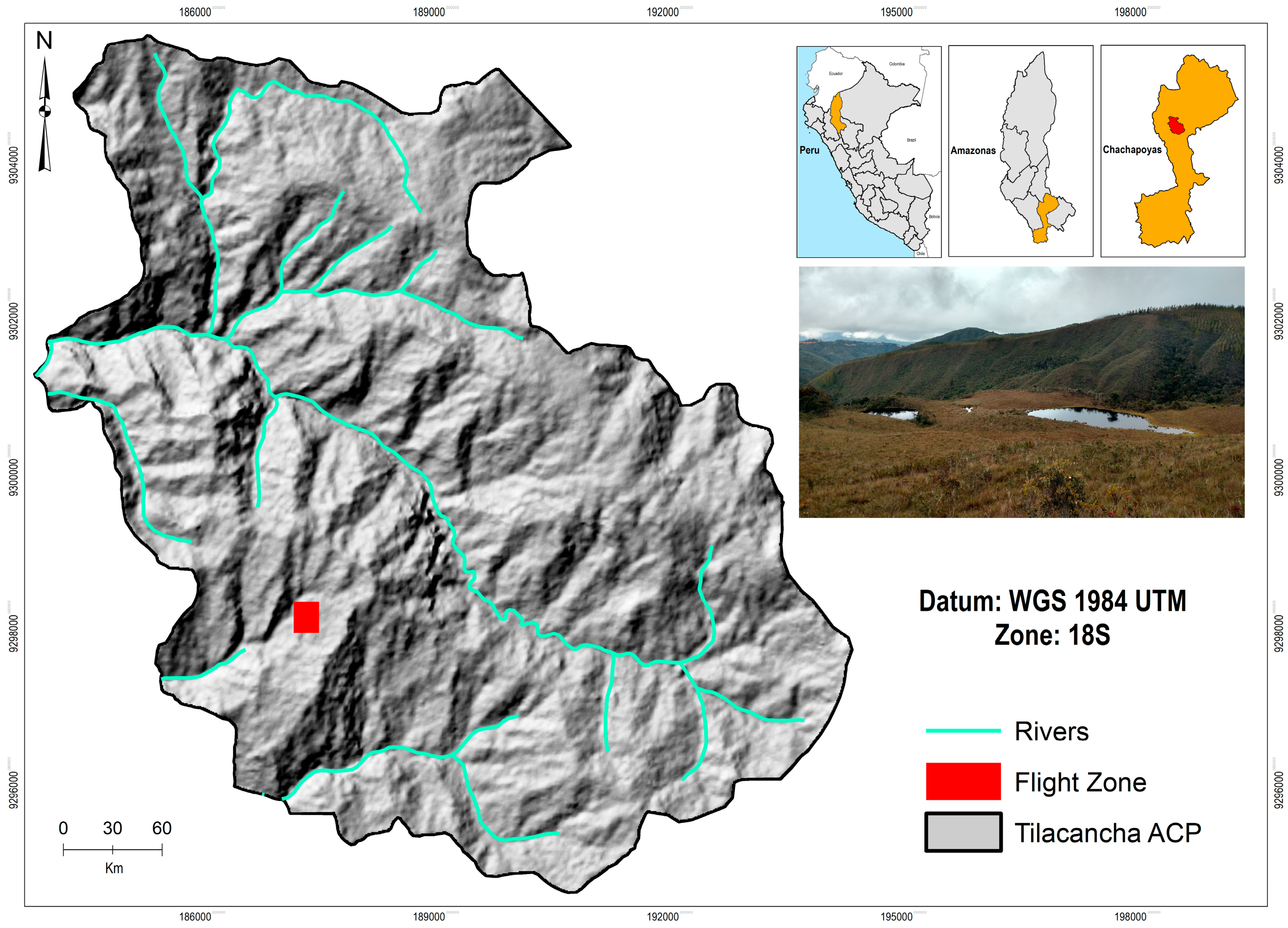
2.1. Study Area Location

The four lakes (A, B, C, and D) are in the Tilacancha PCA (Figure 1). This area is located between 2700 and 3490 m.a.s.l. in the stream of the same name, within the Utcubamba River basin, a tributary of the Marañón River, in the Amazon region of Peru (Figure 1). This PCA is located on lands of the communities of Levanto and San Isidro de Maino, and it has an area of 6800.48 ha [35]. The flight zone had the following cover types: water bodies, relict and shrub forests, pine forests, grassland, bare soil, and construction zones. A radio of 180 m was established in the grassland area for the landing of the Parrot Disco-Pro Ag drone. Table 1 shows the geographic coordinates for the centroids of the irregular polygons of the four lakes; these coordinates were extracted using ArcGIS software ver. 10.7. Likewise, the areas in square meters (m2) are presented for the four lakes, where lake A is the largest, followed by lakes C, B, and D.

2.2. Data Acquisition and UAV Image Processing

A Parrot Sequoia multispectral camera was used in this investigation (Table 2), as well as a Parrot Disco-Pro AG fixed-wing drone. The Parrot Sequoia multispectral sensor features four bands, green (550 nm), red (660 nm), near infrared (790 nm), and red edge (735 nm), and captures visible and invisible images. This multispectral camera was developed for agricultural purposes for its ability to evaluate photosynthetic processes; it also features a sunlight sensor for calibration and a 16-megapixel RGB camera. The multispectral camera is independent of the drone and features a standard protocol (PTP) for communication with drones and is powered by a USB connection.
The Parrot Disco-Pro AG has a fixed-wing flight mode allowing a linear type of movement. It has relatively long flight times of 45 min and covers, on average, an area of 80 ha at sea level, which solves the disadvantage of rotary wing or multi-rotor UAVs [36].

2.2.1. Flight Programming

The flight day took place in the lake sector of the Tilacancha PCA on 1 December 2021 at 12:15:33 p.m. at Mountain Standard Time with a duration of 00:05:56 min. As a flight reference, we have the following geographic coordinates: −6.341022, −77.824907, with an altitude from 2996.30 to 3142.38 m.a.s.l. The flight altitude, on average, of the drone was 100 m, generating a resolution of 17.80 cm for the RGB band and multispectral images.
The flight was programmed using Pix4D Capture 4.10 software. In the settings function, the Disco-Pro AG drone was selected. Next, adjustments were made to the flight plan with the following parameters: a camera angle of 90°; for the images provided by the multispectral camera, a frontal overlap of 80% was made and a lateral overlap of 70%, with a flight altitude of 100 m at 60 km/h. While operating the UAV, the doubling rate, flight time, and flight altitude were set to 80%.

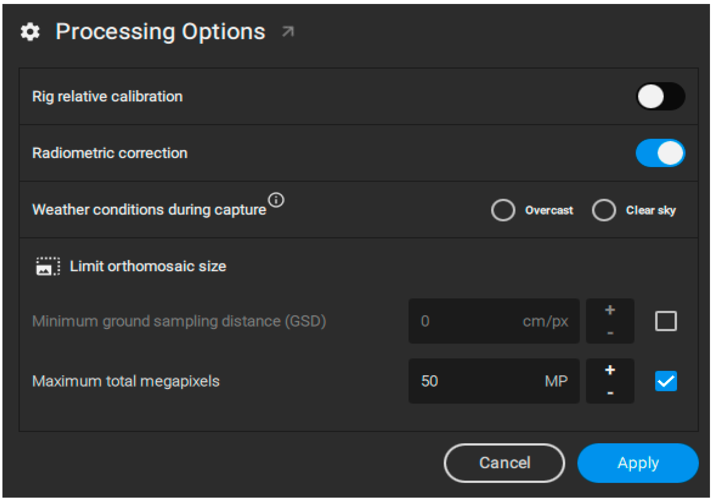
2.2.2. Radiometric Calibration of the Parrot Sequoia Camera

Radiometric calibration is an essential step in UAV data processing, especially when acquiring images for the analysis of biophysical processes [37]. Kelcey and Lucieer cover techniques used to reduce the effects of relative environmental variables and extract absolute reflectance measurements from the data [38]. Because the manufacturer’s methods are often easier and faster to implement than empirical methods, and do not require additional work or expert knowledge to generate calibrated images [39], for this research, radiometric calibration of the multispectral images obtained from the Parrot Sequoia camera was performed automatically in Pix4DFields 1.8.1 software [32]. Pix4Dfields performs different types of radiometric correction, depending on the availability of the following sources of information: sunlight sensors and weather conditions. The weather conditions during capture are important as the Pix4Dfields program allows the user to enter this information (Figure 2). Therefore, it is important to note and save the weather conditions, such as clear or cloudy skies, during which a data set is acquired. For the daytime flight, cloudy sky conditions were used.

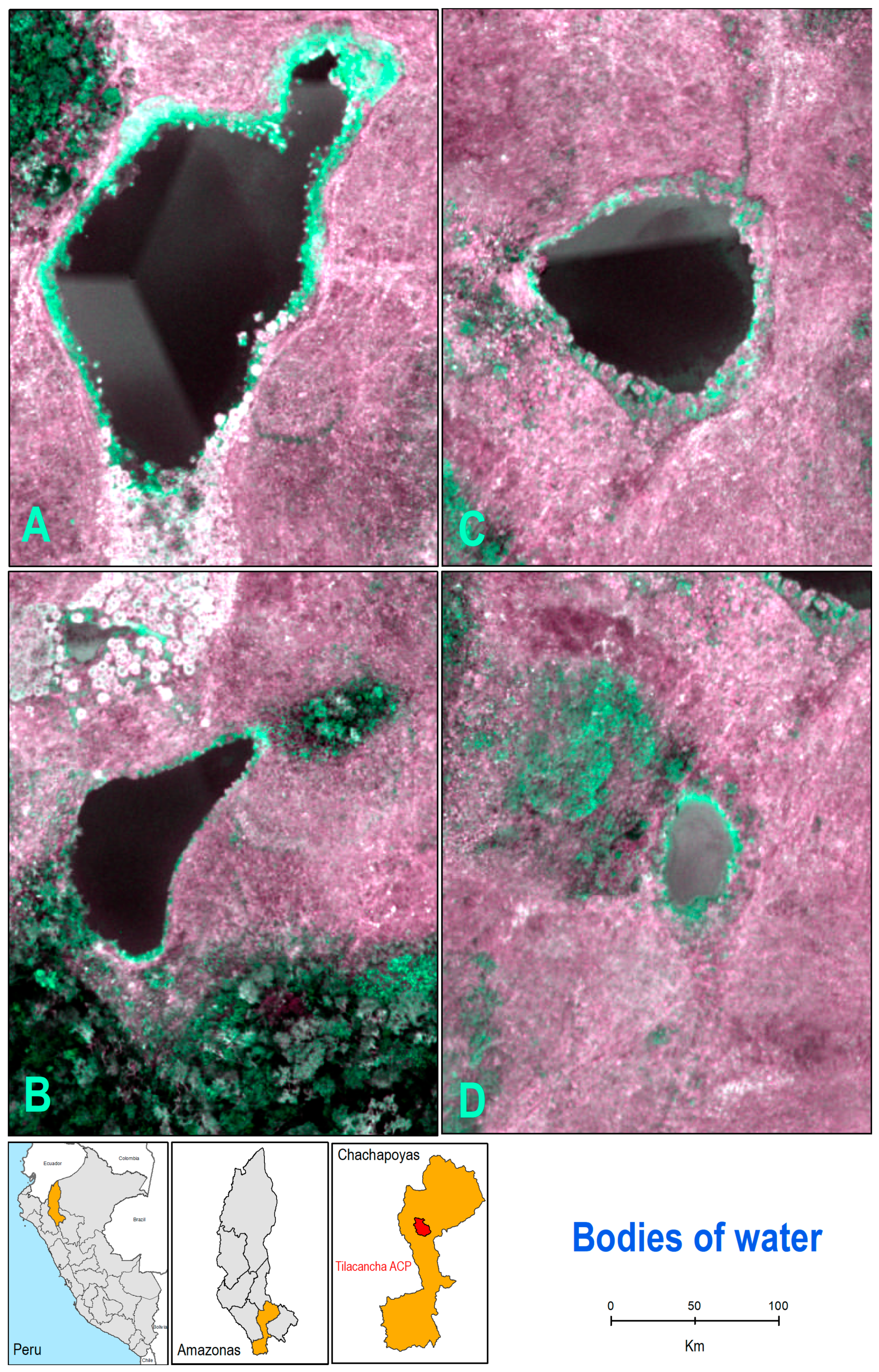
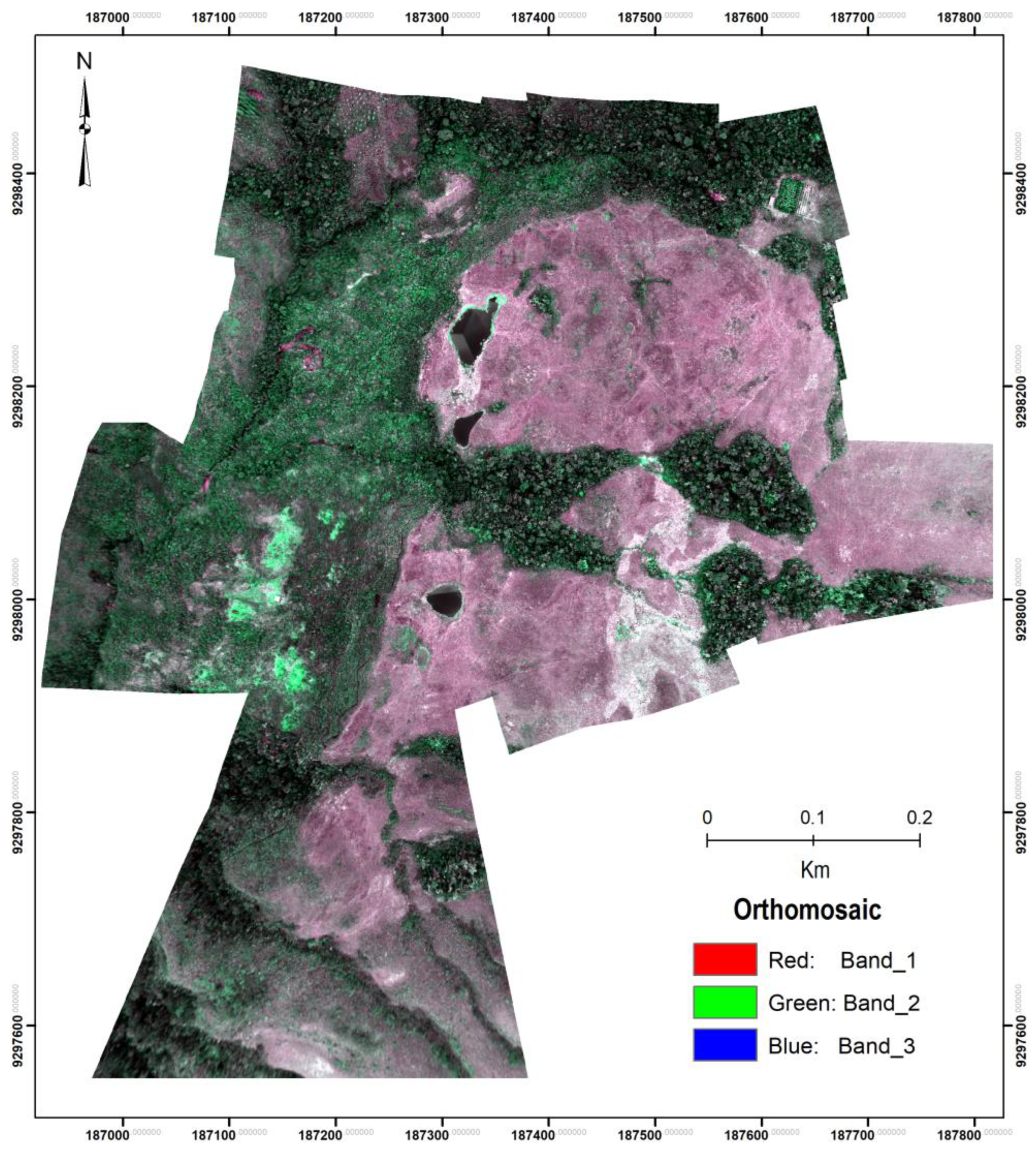
2.2.3. Orthomosaic and Lake Extraction

With the flight of the Parrot Disco-Pro Ag drone, 338 images were acquired for each spectral wavelength band. In the construction of the orthomosaic, 288 multispectral images as TIFF files captured at a flight altitude of 100 m were used. The images were then processed to create an orthomosaic of the flight area (Figure 3) using Pix4Dfields software, which uses a direct-to-orthomosaic photogrammetry pipeline optimized for fast processing of smooth terrain from drone imagery. In addition, 10 field control points were established for the construction of the orthomosaic; these points were made with a differential GPS (Trimble R12) where the horizontal error was estimated to be 11.2 cm between the points in the field and the points in the orthomosaic (root mean square error—RMSE) using Excel 2021 software. Previously the geographic coordinates were transformed to UTM coordinates for zone 18 S using ArcGIS 10.7 software (Reproject function).

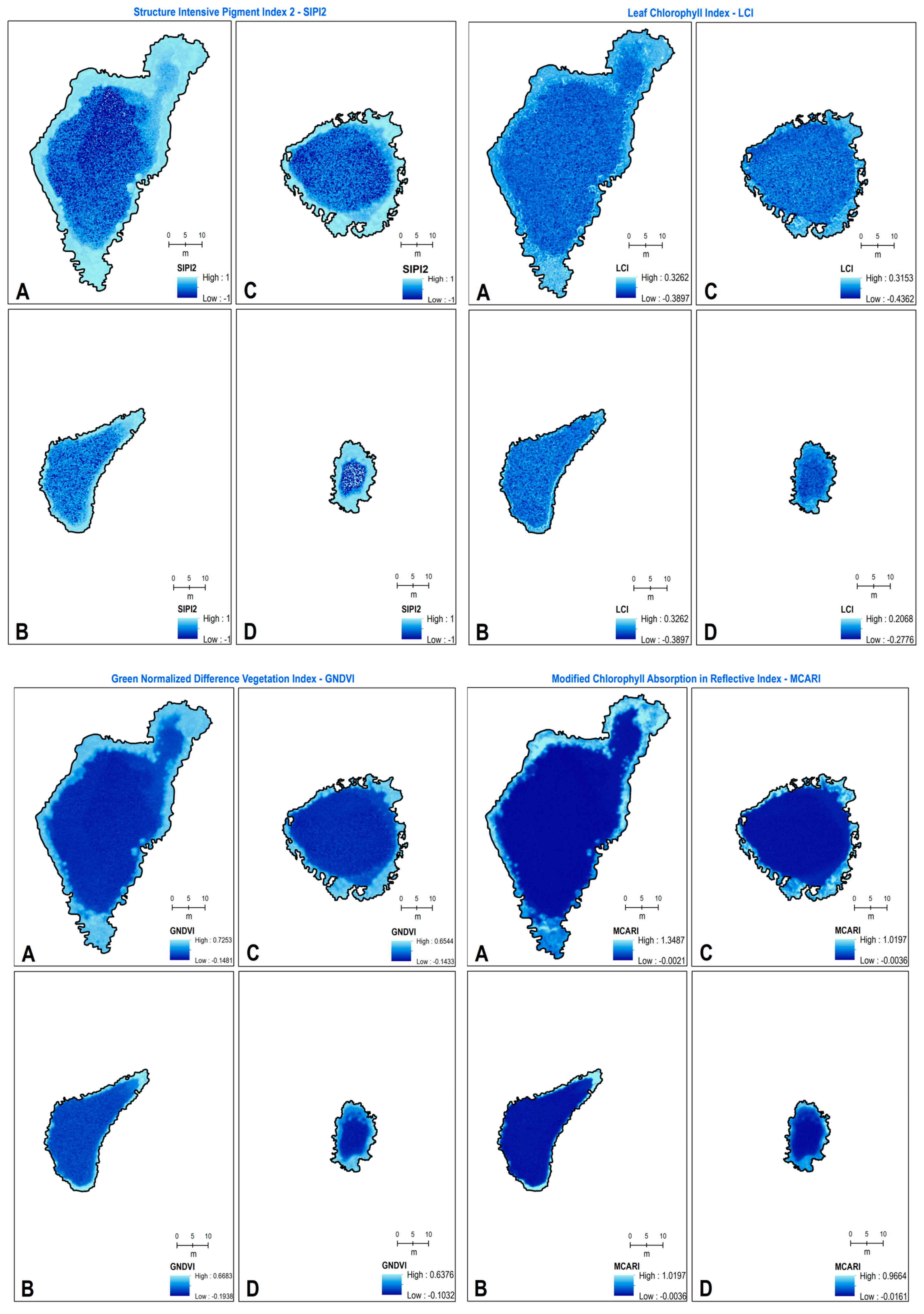
2.2.4. Vegetation Spectral Indexes

For the four lakes, a total of six vegetation indexes were analyzed (Table 3). These indexes were selected for their potential to extract vegetation areas in previous studies and can be analyzed using the spectral wavelength bands acquired from the Sequoia multispectral sensor using Pix4Dfields software. For the analysis of vegetation indexes, the Raster Calculator tool from ArcGIS 10.7 software was applied to the orthoimages of each spectral wavelength band, as shown in Table 2.

2.3. Statistical Methodology

After obtaining the values per pixel for each index for the four lakes, statistical analysis was performed to determine differences in mean values for each vegetation index. For the pixels for the four lakes, the maximum, minimum, average, and standard deviation values for each vegetation index were identified. The level of sensitivity of each vegetation index was analyzed as a ratio between the standard deviation of the index to its mean value [40].
Regarding the comparison between lakes, we first analyzed whether the variables (vegetation indexes) had normally distributed data. The normality test was performed using the Kolmogorov–Smirnov goodness-of-fit statistic (p ≤ 0.01); this test is used with more robustness for large samples [44]. This test made it possible to analyze the distribution of the values of each pixel using histograms and normal Q–Q plots made for each vegetation index (https://www.r-project.org/, accessed on 19 January 2021).
The maximum, minimum, and standard deviation values for the total number of pixels for each lake were characterized. Levene’s approach is powerful and robust to non-normality and has become a popular tool for verifying the equality of variances (homogeneity of variances [45]) and was therefore used in this research.
An analysis of variance (ANOVA) was then applied, and the performance of the procedure was evaluated with its family error rate and its power under different distributions [46] using R 4.1.2 software [28]. Next, a comparison between the means was carried out by performing Tukey’s honest significant difference (HSD) test (https://www.r-project.org/, accessed on 19 January 2021). This is a multiple-comparison statistical procedure to evaluate multiple means, where no assumptions about distribution, sample size, or homogeneity of variance are necessary [28]. The Tukey–Kramer HSD test compared all possible pairs of means of the four lakes in the Tilacancha PCA, where we considered the same sample size for the four lakes and subsequent analysis of means for the six vegetation indices.

3. Results and Discussion

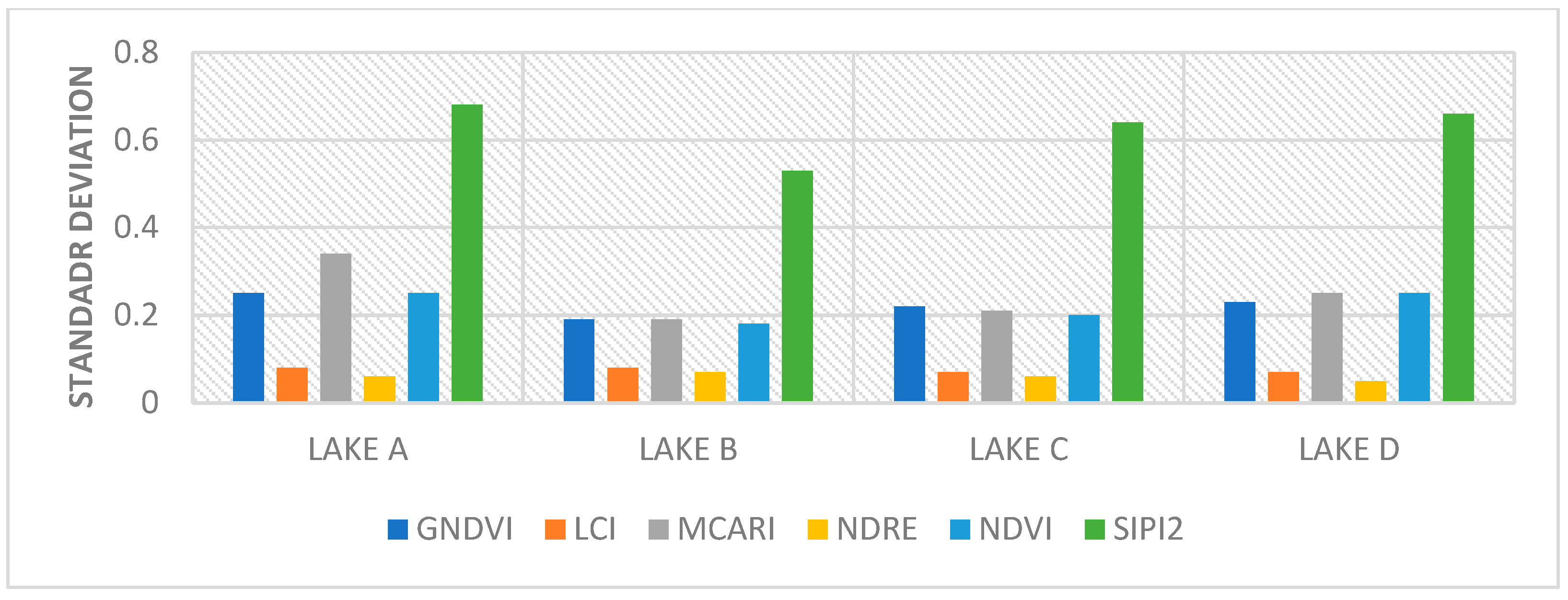
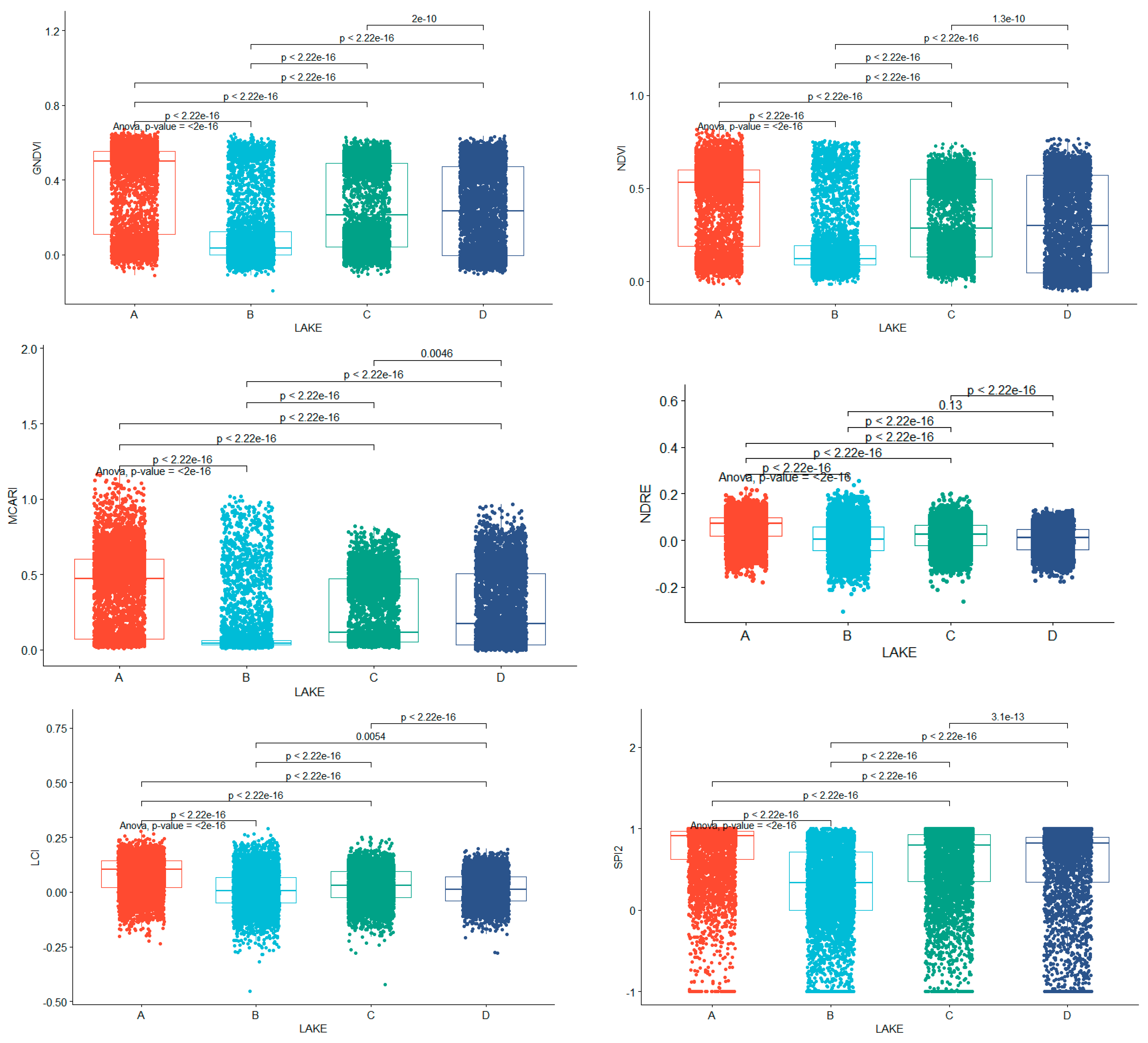
3.1. Sensitivity between Indexes for the Lakes

For each lake, Figure 4 shows the level of sensitivity of the six vegetation indexes, determined as a ratio between the standard deviation of each index to its mean value. The four lakes presented the highest SD values in the SIPI2, i.e., it corresponds to the index with the highest sensitivity compared to the others. The SIPI2 had an SD up to 13.20 higher (in lake D) compared to the lowest deviation value (0.05 for the NDRE) among the six indexes. Likewise, in the four lakes, the lowest level of sensitivity was for the NDRE index, with a minimum SD of 0.05 (lake D) (Figure 5).

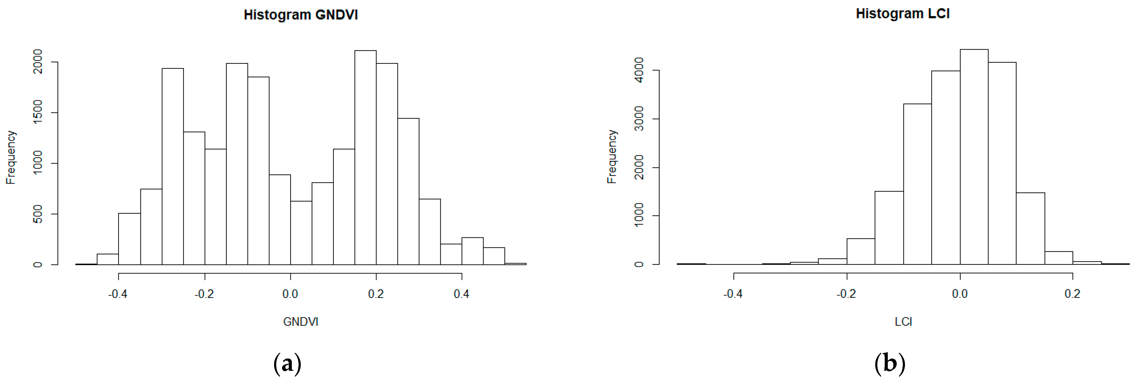
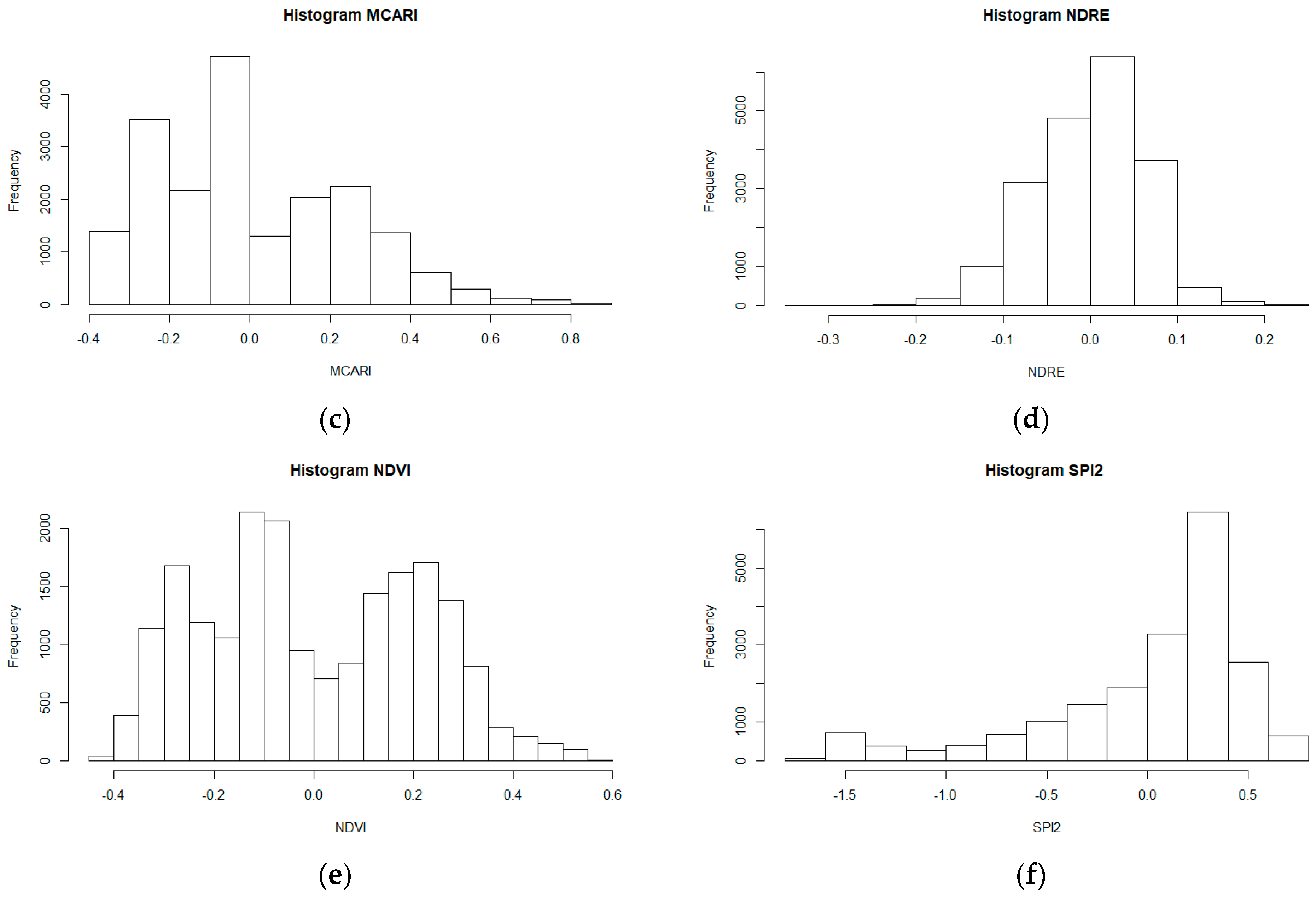
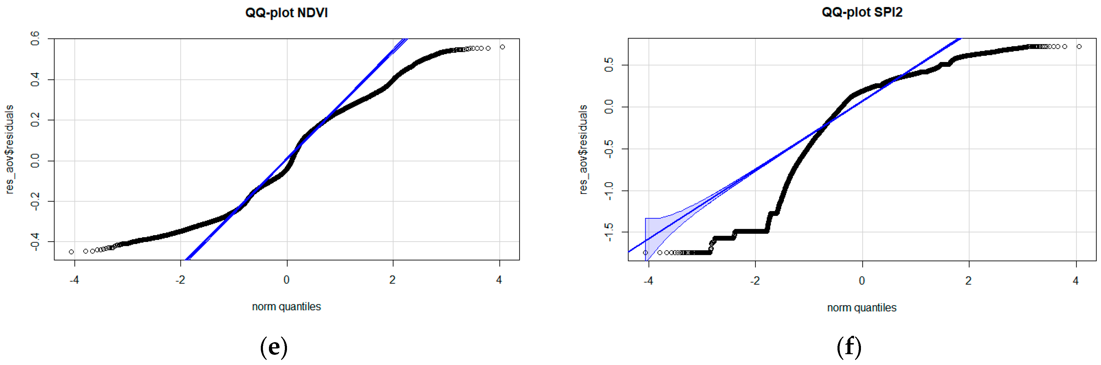
3.2. Reporting the Results of the Normality Test of Multivariables between Four Lakes

The frequency histogram and Q–Q plot showed that the shapes and distribution trends of the pixel values were different according to the six vegetation indexes (Figure 6 and Figure 7). In this sense, the GNDVI (Figure 6a) and the NDVI (Figure 6e) presented multimodal data. However, the LCI, MCRI, NDRE, and SIP2 plots were skewed (Figure 6b, 6c, 6d and 6f, respectively). Next, the Q–Q plots for each index were analyzed.
The Q–Q plots for the LCI and the NDRE (Figure 7b,d) showed that the points did not deviate too far from the 1:1 line. Likewise, they presented a few atypical values for the LCI and NDRE. Finally, these plots suggested a possible lack of fit in the tails, but these were not huge. Otherwise, the GNDVI, the MCRI, and the NDVI (Figure 7a, Figure 7c and Figure 7d, respectively) presented as heavy-tailed data. Finally, plot 3f is of the left-skewed data type. Visually, the only Q–Q plots that supposedly showed normality are 8b (LCI) and 8d (NDRE); however, the Kolmogorov–Smirnov test (Table 4) corroborated the assumptions in the histogram and Q–Q plot data. Since the values were greater than 0.05, the data were found to be within a normal distribution in all cases.

3.3. Equality of Variances—Homogeneity

Maximum values, minimum values, and standard deviations were determined for the six vegetation indexes (GNDVI, LCI, MCARI, NDRE, NDVI, and SPI2) in the total number of pixels for the four lakes, as shown in Table 4. The ranges of values of all vegetation indexes are represented in ranges from −1 to 1. The SPI2 was the only index that presented extreme range values for the four lakes. The highest standard deviations were found for the SPI2, and the lowest standard deviations were found for the NDRE index.
An analysis of variance (ANOVA) was then applied, and the performance of the procedure was evaluated with its family error rate. Table 4 shows the values of the family error rate, where all vegetation indexes and significant statistical differences were obtained between lakes (p-values < 0.001). Levene’s test is less sensitive to deviations from normality. Next, we proceeded to perform pairwise comparisons of lakes for the six vegetation indexes using the Tukey HSD test. This statistic was used to find means that were significantly different from each other in this case for the vegetation indices in the four lakes. According to Table 4, there was strong (p-values < 0.001) evidence against the null hypothesis, which was the equal variance assumption for the six vegetation indices for the four lakes.

3.4. Tukey HSD Tests

Table 5 and Figure 8 show comparisons by pairs of lakes for the six vegetation indexes evaluated at a given time.
For the six vegetation indexes for the four lakes, there was strong evidence against the null hypothesis—that the mean difference is zero between two lakes compared for each index—but not when evaluating the mean of the LCI between lakes B and D, because there was moderate (p-value 0.0303) evidence against the null hypothesis—that the mean difference for the LCI is zero between the two lakes B and D. Also, for the NDRE, there was no evidence (p-value 0.408) against the null hypothesis for lakes D and B—that the mean difference is zero.
In the Green Normalized Difference Vegetation Index (GNDVI), significant statistical differences between pairs of lakes were shown for all cases (lakes: A-B, C-A, D-A, C-B, D-B, and D-C). In other words, the photosynthetic rates allowed determining different conditions of changes in photosynthetic organisms in each lake.
When comparing the Leaf Chlorophyll Index (LCI), significant differences were shown between the pairs of lakes: A-B, C-A, D-A, C-B, D-B, and D-C. Thus, the chlorophyll content in areas of cover with photosynthetic microorganisms between lakes is different.
In the same sense, the Modified Chlorophyll Absorption in Reflective Index (MCARI) showed statistical differences between all pairs of lakes (A-B, C-A, D-A, C-B, D-B, and D-C). It was then deduced that chlorophyll concentrations and leaf area index variations differ between pairs of lakes.
The values for the Normalized Difference Red Edge (NDRE) presented statistical differences for the following pairs of lakes: A-B, C-A, D-A, C-B, and D-C. That is, the index was sensitive to the chlorophyll content in photosynthetic microorganisms against soil background effects. The D-B lake pair showed no statistical significance, indicating that despite mathematical differences, the response to the behavior of plants in the NDRE does not differ between these lakes.
There were significant statistical differences for all pairs of lakes when we evaluated the Normalized Difference Vegetation Index (NDVI). We determined that the measure of green vegetation cover and the health of the vegetation in the lakes differ from each other.
Finally, significant differences in the Structure Intensive Pigment Index 2 (SIPI2) allowed us to determine that the zones with great variability in the canopy structure differ among all the lakes.
The potential use of the six vegetation indexes evaluated in this work lies in the fact that remote sensing methods with UASs and multispectral cameras provide synoptic and spatiotemporal views with a higher level of accuracy, and their integration can lead to a better understanding of lake ecology and water quality [15]. Likewise, the ranges of values obtained in each index, as well as the dynamics of data dispersion demonstrated in the frequency histograms and Q–Q plots, were based on the measurement of the radiation reflected by photosynthesizing biological beings and have the potential to assess the status of many plants within the field of view of the sensor [41]. Although at the water surface, radiation is reflected or passes through the water surface according to Snell’s law and propagates through the water mass [15], statistical differences were obtained in the vegetation indexes evaluated in this research on lakes, which could be determined by changes in the chlorophyll concentration, allowing us to corroborate that they do not affect all parts of the visible reflectance spectrum equally [47]. Thus, there will be independent variation in the structure and function of vegetation, as suggested by [48].
By determining the wavelengths of each band within the electromagnetic spectrum, significant variations in SD were achieved concerning sensitivity and significant statistical differences between indexes and between the pixels of the assessed lakes. Thus, in addition to the NDVI and the GNDVI, already suggested in other research as effective for detecting aquatic plants when using UAV imagery [36], we consider important future uses and evaluation of potentialities for the LCI, the MCARI, the NDRE, and the SPI2 on the dynamics of aquatic ecosystems of the Peruvian Jalca. However, research considers that the reliability of spectral information acquired by multispectral sensors mounted on UAVs is not completely clear [49].
Because absolute accuracy may be insufficient for some applications, future calibration procedures will be required [50], as well as validation of indexes, such as the MCARI, commonly used to minimize the combined effects of soil reflectance and non-photosynthetic materials [51]. In addition, the value of the vegetation indexes should be identified according to the pool of photosynthetic organisms in bodies of water, which should be studied continuously in the future [36], contrasting with molecular characterization of aquatic photosynthetic species.
Vegetation spectral indexes can increase linearly with the photosynthetic potential of the vegetation [47]. For example, the NDVI is not sensitive to higher chlorophyll concentrations or photosynthetic rates for a large vegetation cover [40], but it is sensitive to low chlorophyll concentrations, to the fraction of plant cover, and, as a result, to the absorbed photosynthetically active solar radiation [47]. The GNDVI can be used to detect vegetation conditions with high accuracy using a variety of the “green” channels [40]. The MCARI is used as a measure of green biomass [52] and presents a solid theoretical basis as a measure of the photosynthetically active solar radiation absorbed by the canopy [53,54]. The NDRE shows chlorophyll levels associated with indicating nitrogen limitation in the leaves [55], while the LCI is a promising alternative for soil nitrate testing [56].
Investigating differences between the means of more than two groups or experimental conditions is a routine research question addressed in biology [28]. The results of this research will encourage future studies to observe time-dependent trends in the proliferation of photosynthetic organisms over water bodies using the methodologies described for the first time, added to research of this nature. In addition, spectral wavelength bands and vegetation indexes should be further analyzed for careful use [36] in making decisions that require water management and conservation. The practical merits of the family error rate and its power under different distributions have been tested in multiple statistical comparisons. Although it does not need assumptions about the distribution, this research performed the homogeneity test to demonstrate in the first instance the distribution of pixels in each lake according to ranges and between lakes, despite the closeness of the lakes.

4. Conclusions

It was possible to use as hardware (HW) a Parrot Sequoia multispectral camera (four-band) mounted on a Parrot Disco-Pro Ag drone and the software (SW) Pix4DFields 1.8.1 to obtain six vegetation indexes for four lakes in the lakes sector of the Tilacancha PCA in the Peruvian Jalca.
Since the pixels for the four lakes in this study were randomly selected for a comparison of the means of the flight conducted in December 2021 in the Tilacancha PCA lake sector, the four lakes observed in this study by researchers of the Drone Project-UNTRM are limited. Finally, since this was an observational study, it was not possible to establish a causal relationship between the pixel and the mean of its value for each vegetation index.
The sensitivity and dispersion of values obtained from the camera images helped to discriminate more accurately the distribution of pixel ranges. The SIPI2 obtained the highest level of sensitivity concerning the degree of pixel distribution in the ranges shown in the histogram according to the standard deviation; however, the values of all the indexes were not disregarded, because they showed statistical differences between gaps despite their closeness. The family error rate and Tukey–Kramer HSD statistics (means) allowed for establishing statistical differences between pairs of lakes for all cases. Proposals for the management and conservation of such important and close lakes must be made on an individual basis to provide sustainable water quality. Future DNA research and calibration of the UAVs and software are necessary to determine the pool of microorganisms with photosynthetic activity present in each lake and thus provide high-level targeted strategies.
Finally, the global pattern and distribution of most freshwater taxonomic groups in response to climate change are still unknown and require further research. Understanding the variation in biodiversity trends in response to biotic and abiotic threats and consolidating knowledge are crucial to maintaining freshwater ecosystem services [57], and indexes used for forest and agricultural ecosystems can be used to monitor habitat changes in aquatic ecosystems at high resolution [36]. Drones can greatly support field studies in plant species monitoring by enabling accurate species mapping and high-resolution images captured just in time [33]. The aquatic ecosystems of the Peruvian Jalca can be better managed under an integrated approach, contributing to the SDG6.

Author Contributions

Conceptualization, J.V., L.G., S.C. and M.O.; methodology, J.V. and L.G.; software, J.V., L.G. and S.C.; validation, J.V., L.G., J.L.M. and S.C.; formal analysis, J.V. and L.G.; investigation, J.V. and S.C.; resources, J.V., S.C. and M.O.; data curation, J.V., E.A., J.L.M. and L.G.; writing—original draft preparation, J.V., L.G., S.C., E.A. and M.O.; writing—review and editing, J.V., L.G., S.C., E.A. and M.O.; visualization, J.V., J.L.M. and M.O.; supervision, S.C. and M.O.; project administration, J.V., S.C., J.L.M. and M.O.; funding acquisition, J.V., L.G., S.C., J.L.M. and M.O. All authors have read and agreed to the published version of the manuscript.

Funding

The study was funded by the Instituto de Investigación para el Desarrollo Sustentable de Ceja de Selva (INDES-CES) in the project named “Creación de los Servicios del Centro de Investigación, innovación y Transferencia Tecnológica de Café de la Universidad Nacional Toribio Rodríguez de Mendoza de Amazonas” (C.U.I. N° 2317883—CEINCAFÉ) and the project named “Análisis de la cobertura vegetal, cuerpos de agua, erosión de suelo y monitoreo de invasiones de territorio empleando dos tipos de drones en el área de conservación privada Tilacancha” (CONTRATO N° 161-2018-FONDECYT-BM-IADT-SE), Universidad Nacional Toribio Rodríguez de Mendoza de Amazonas del Perú.

Data Availability Statement

Not applicable.

Acknowledgments

Thanks to the Universidad Nacional Toribio Rodríguez de Mendoza de Amazonas (UNTRM) for research support and economic funds in the PROCEPIT project.

Conflicts of Interest

The authors declare no conflict of interest.

References

  1. Ministerio del Ambiente de Perú (MINAM). Mapa Nacional de Ecosistemas del Perú. Dirección General de Ordenamiento Territorial Ambiental—DGOTA. 2019. Available online: https://sinia.minam.gob.pe/mapas/mapa-nacional-ecosistemas-peru (accessed on 19 January 2021).
  2. Ruiz, D.; Moreno, H.A.; Gutiérrez, M.E.; Zapata, P.A. Changing Climate and Endangered High Mountain Ecosystems in Colombia. Sci. Total Environ. 2008, 398, 122–132. [Google Scholar] [CrossRef]
  3. Aparecido, L.M.T.; Teodoro, G.S.; Mosquera, G.; Brum, M.; Barros, F.d.V.; Pompeu, P.V.; Rodas, M.; Lazo, P.; Müller, C.S.; Mulligan, M.; et al. Ecohydrological Drivers of Neotropical Vegetation in Montane Ecosystems. Ecohydrology 2018, 11, e1932. [Google Scholar] [CrossRef]
  4. Hofstede, R.; Calles, J.; López, V.; Polanco, R.; del Torres, F.; Ulloa, J.; Vásquez, A.; Cerra, M. Los Páramos Andinos ¿Qué Sabemos? UICN: Quito, Ecuador, 2014; ISBN 9789978993293. Available online: https://portals.iucn.org/library/sites/library/files/documents/2014-025.pdf (accessed on 19 January 2021).
  5. Ochoa-Sánchez, A.; Crespo, P.; Carrillo-Rojas, G.; Sucozhañay, A.; Chandler, D.G.; Célleri, R. Actual Evapotranspiration in the High Andean Grasslands: A Comparison of Measurement and Estimation Methods. Front. Earth Sci. 2019, 7, 55. [Google Scholar] [CrossRef]
  6. Ricardi, M.; Gaviria, J.; Estrada, J. La Flora Del Superpáramo Venezolano y Sus Relaciones Fitogeográficas a Lo Largo de Los Andes. Plantula 1997, 1, 171–187. Available online: https://www.researchgate.net/publication/26409727_La_Flora_del_Superparamo_venezolano_y_sus_relaciones_fitogeograficas_a_lo_largo_de_Los_Andes (accessed on 19 January 2021).
  7. Galán de Mera, A.; Sánchez Vega, I.; Montoya Quino, J.; Linares Perea, E.; Campos de la Cruz, J.; Vicente Orellana, J.A. BOSQUES A LA JALCA EN CAJAMARCA. Acta Bot. Neerl. 2015, 40, 157–190. [Google Scholar]
  8. Weberbauer, A. El Mundo Vegetal de Los Andes Peruanos. Estudio Fitogeográfico; Ministerio de Agricultura: Lima, Perú, 1945.
  9. Faghihinia, M.; Xu, Y.; Liu, D.; Wu, N. Freshwater biodiversity at different habitats: Research hotspots with persistent and emerging themes. Ecol. Indic. 2021, 129, 107926. [Google Scholar] [CrossRef]
  10. Angelakis, A.N.; Valipour, M.; Choo, K.-H.; Ahmed, A.T.; Baba, A.; Kumar, R.; Toor, G.S.; Wang, Z. Desalination: From Ancient to Present and Future. Water 2021, 13, 2222. [Google Scholar] [CrossRef]
  11. Lynch, A.J.; Cooke, S.J.; Deines, A.M.; Bower, S.D.; Bunnell, D.B.; Cowx, I.G.; Nguyen, V.M.; Nohner, J.; Phouthavong, K.; Riley, B.; et al. The Social, Economic, and Environmental Importance of Inland Fish and Fisheries. Environ. Rev. 2016, 24, 115–121. [Google Scholar] [CrossRef]
  12. Brönmark, C.; Hansson, L.A. Environmental Issues in Lakes and Ponds: Current State and Perspectives. Environ. Conserv. 2002, 29, 290–307. [Google Scholar] [CrossRef]
  13. Leveque, C. Lake and Pond Ecosystems. Encycl. Biodivers. 2001, 3, 633–644. Available online: https://horizon.documentation.ird.fr/exl-doc/pleins_textes/divers20-05/010032564.pdf (accessed on 19 January 2021).
  14. Sala, O.E.; Chapin, F.S.; Armesto, J.J.; Berlow, E.; Bloomfield, J.; Dirzo, R.; Huber-Sanwald, E.; Huenneke, L.F.; Jackson, R.B.; Kinzig, A.; et al. Global Biodiversity Scenarios for the Year 2100. Science 2000, 287, 1770–1774. [Google Scholar] [CrossRef]
  15. Dörnhöfer, K.; Oppelt, N. Remote Sensing for Lake Research and Monitoring—Recent Advances. Ecol. Indic. 2016, 64, 105–122. [Google Scholar] [CrossRef]
  16. Moss, B. Biodiversity in Fresh Waters-an Issue of Species Preservation or System Functioning? Environ. Conserv. 2000, 27, 1–4. [Google Scholar] [CrossRef]
  17. Law, A.; Baker, A.; Sayer, C.; Foster, G.; Gunn, I.D.M.; Taylor, P.; Pattison, Z.; Blaikie, J.; Willby, N.J. The Effectiveness of Aquatic Plants as Surrogates for Wider Biodiversity in Standing Fresh Waters. Freshw. Biol. 2019, 64, 1664–1675. [Google Scholar] [CrossRef]
  18. Ecke, F. The Added Value of Bryophytes and Macroalgae in Ecological Assessment of Lakes. Ecol. Indic. 2018, 85, 487–492. [Google Scholar] [CrossRef]
  19. O’Hare, J.M.; O’Hare, M.T.; Gurnell, A.M.; Scarlett, P.M.; Liffen, T.; Mcdonald, C. Influence of an Ecosystem Engineer, the Emergent Macrophyte Sparganium Erectum, on Seed Trapping in Lowland Rivers and Consequences for Landform Colonisation. Freshw. Biol. 2012, 57, 104–115. [Google Scholar] [CrossRef]
  20. Guo, J.-L.; Yu, Y.-H.; Zhang, J.-W.; Li, Z.-M.; Zhang, Y.-H.; Volis, S. Conservation strategy for aquatic plants: Endangered Ottelia acuminata (Hydrocharitaceae) as a case study. Biodivers. Conserv. 2019, 28, 1533–1548. [Google Scholar] [CrossRef]
  21. Bullerjahn, G.S.; McKay, R.M.L.; Bernát, G.; Prášil, O.; Vörös, L.; Pálffy, K.; Tugyi, N.; Somogyi, B. Community dynamics and function of algae and bacteria during winter in central European great lakes. J. Great Lakes Res. 2019, 46, 732–740. [Google Scholar] [CrossRef]
  22. Maslennikova, A.V. Development and Application of an Electrical Conductivity Transfer Function, Using Diatoms from Lakes in the Urals, Russia. J. Paleolimnol. 2020, 63, 129–146. [Google Scholar] [CrossRef]
  23. Altschul, D.; Buchholz, K. Water-Born Micro-Cities: Bringing the Great Lakes Closer to Natural Symbiosis with Eco-Based Design. Plan J. 2017, 2, 87–104. [Google Scholar] [CrossRef]
  24. Incagnone, G.; Marrone, F.; Barone, R.; Robba, L.; Naselli-Flores, L. How Do Freshwater Organisms Cross the “Dry Ocean”? A Review on Passive Dispersal and Colonization Processes with a Special Focus on Temporary Ponds. Hydrobiologia 2015, 750, 103–123. [Google Scholar] [CrossRef]
  25. Naselli-Flores, L.; Padisák, J.; Albay, M. Shape and Size in Phytoplankton Ecology: Do They Matter? Hydrobiologia 2007, 578, 157–161. [Google Scholar] [CrossRef]
  26. Main, R.; Cho, M.A.; Mathieu, R.; O’Kennedy, M.M.; Ramoelo, A.; Koch, S. An Investigation into Robust Spectral Indices for Leaf Chlorophyll Estimation. ISPRS J. Photogramm. Remote Sens. 2011, 66, 751–761. [Google Scholar] [CrossRef]
  27. Ritchie, J.C.; Zimba, P.V.; Everitt, J.H. Remote Sensing Techniques to Assess Water Quality. Photogramm. Eng. Remote Sens. 2003, 69, 695–704. [Google Scholar] [CrossRef]
  28. Herberich, E.; Sikorski, J.; Hothorn, T. A Robust Procedure for Comparing Multiple Means under Heteroscedasticity in Unbalanced Designs. PLoS ONE 2010, 5, e9788. [Google Scholar] [CrossRef] [PubMed]
  29. Schaeffer, B.A.; Schaeffer, K.G.; Keith, D.; Lunetta, R.S.; Conmy, R.; Gould, R.W. Barriers to Adopting Satellite Remote Sensing for Water Quality Management Barriers to Adopting Satellite Remote Sensing for Water Quality Management. Int. J. Remote Sens. 2013, 34, 7534–7544. [Google Scholar] [CrossRef]
  30. Singgih, I.K.; Lee, J.; Kim, B. Node and Edge Drone Surveillance Problem With Consideration of Required Observation Quality and Battery Replacement. IEEE Access 2020, 8, 44125–44139. [Google Scholar] [CrossRef]
  31. Matthews, M.W.; Bernard, S.; Winter, K. Remote Sensing of Cyanobacteria-Dominant Algal Blooms and Water Quality Parameters in Zeekoevlei, a Small Hypertrophic Lake, Using MERIS. Remote Sens. Environ. 2010, 114, 2070–2087. [Google Scholar] [CrossRef]
  32. Franzini, M.; Ronchetti, G.; Sona, G.; Casella, V. Geometric and Radiometric Consistency of Parrot Sequoia Multispectral Imagery for Precision Agriculture Applications. Appl. Sci. 2019, 9, 5314. [Google Scholar] [CrossRef]
  33. Oldeland, J.; Revermann, R.; Luther-Mosebach, J.; Buttschardt, T.; Lehmann, J.R.K. New tools for old problems—Comparing drone- and field-based assessments of a problematic plant species. Environ. Monit. Assess. 2021, 193, 90. [Google Scholar] [CrossRef] [PubMed]
  34. Oldeland, J.; Große-Stoltenberg, A.; Naftal, L.; Strohbach, B.J. The Potential of UAV Derived Image Features for Discriminating Savannah Tree Species. In The Roles of Remote Sensing in Nature Conservation; Springer International Publishing: Berlin/Heidelberg, Germany, 2017; pp. 183–201. [Google Scholar]
  35. Ministerio del Ambiente de Perú (MINAM). MINAM Resolución Ministerial N° 118-2010-MINAM 2010, 6. Available online: https://www.minam.gob.pe/disposiciones/resolucion-ministerial-n-118-2010-minam/ (accessed on 1 February 2021).
  36. Song, B.; Park, K. Detection of Aquatic Plants Using Multispectral UAV Imagery and Vegetation Index. Remote Sens. 2020, 12, 387. [Google Scholar] [CrossRef]
  37. Iqbal, F.; Lucieer, A.; Barry, K. European Journal of Remote Sensing Simplified Radiometric Calibration for UAS-Mounted Multispectral Sensor. Eur. J. Remote Sens. 2018, 51, 301–313. [Google Scholar] [CrossRef]
  38. Kelcey, J.; Lucieer, A. Sensor Correction and Radiometric Calibration of a 6-Band Multispectral Imaging Sensor for UAV Remote Sensing. ISPRS Int. Arch. Photogramm. Remote Sens. Spat. Inf. Sci. 2012, XXXIX-B1, 393–398. [Google Scholar] [CrossRef]
  39. Poncet, A.M.; Knappenberger, T.; Brodbeck, C.; Fogle, M.; Shaw, J.N.; Ortiz, B.V. Multispectral UAS Data Accuracy for Different Radiometric Calibration Methods. Remote Sens. 2019, 11, 1917. [Google Scholar] [CrossRef]
  40. Gitelson, A.A.; Kaufman, Y.J.; Merzlyak, M.N.; Blaustein, J. Use of a Green Channel in Remote Sensing of Global Vegetation from EOS-MODIS; Elsevier Science Inc.: Amsterdam, The Netherlands, 1995; Volume 58. [Google Scholar]
  41. T Daughtry, C.S.; Walthall, C.L.; Kim, M.S.; Brown de Colstoun, E.; McMurtrey, J.E., III. Estimating Corn Leaf Chlorophyll Concentration from Leaf and Canopy Reflectance; Elsevier Science Inc.: Amsterdam, The Netherlands, 1999; Volume 74. [Google Scholar]
  42. Filella, I.; Penuelas, J. The red edge position and shape as indicators of plant chlorophyll content, biomass and hydric status. Int. J. Remote Sens. 1994, 15, 1459–1470. [Google Scholar] [CrossRef]
  43. Deering, D.W. Rangeland Reflectance Characteristics Measured by Aircraft and Spacecraft Sensors; ProQuest Dissertations Publishing: Ann Arbor, MI, USA, 1978. [Google Scholar]
  44. Gandica, E. Potencia y Robustez En Pruebas de Normalidad Con Simulación Montecarlo. Rev. Sci. 2020, 5, 108–119. [Google Scholar] [CrossRef]
  45. Gastwirth, J.L.; Gel, Y.R.; Miao, W. The Impact of Levene’s Test of Equality of Variances on Statistical Theory and Practice. Stat. Sci. 2009, 24, 343–360. [Google Scholar] [CrossRef]
  46. Hothorn, T.; Bretz, F.; Westfall, P. Simultaneous Inference in General Parametric Models. Biom. J. 2008, 50, 346–363. [Google Scholar] [CrossRef]
  47. Yoder, B.J.; Waring, R.H. The Normalized Difference Vegetation Index of Small Douglas-Fir Canopies with Varying Chlorophyll Concentrations. Remote Sens. Environ. 1994, 49, 81–91. [Google Scholar] [CrossRef]
  48. Greegor, R.B.; Lytle, F.W.; Chakoumakos, B.C.; Lumpkin, G.R.; Ewing, R.C.; Spiro, C.L.; Wong, J. X-ray Absorption Spectroscopy Investigation of the Ta Site in Alpha-Recoil Damaged Natural Pyrochlores. MRS Online Proc. Libr. 1987, 84, 645–658. [Google Scholar] [CrossRef]
  49. Agapiou, A.; Hadjimitsis, D.G.; Alexakis, D.D. Evaluation of Broadband and Narrowband Vegetation Indices for the Identification of Archaeological Crop Marks. Remote Sens. 2012, 4, 3892–3919. [Google Scholar] [CrossRef]
  50. Hunt, E.R.; Doraiswamy, P.C.; McMurtrey, J.E.; Daughtry, C.S.T.; Perry, E.M.; Akhmedov, B. A Visible Band Index for Remote Sensing Leaf Chlorophyll Content at the Canopy Scale. Int. J. Appl. Earth Obs. Geoinf. 2012, 21, 103–112. [Google Scholar] [CrossRef]
  51. Zarco-Tejada, P.; Sepulcre-Cantó, G. Remote Sensing OF Vegetation Biophysical Parameters FOR Detecting Stress Condition AND Land Cover Changes. Estud. Zona Saturada Suelo 2007, VIII, 37–44. [Google Scholar]
  52. Tucker, C.J. Red and Photographic Infrared Lnear Combinations for Monitoring Vegetation. Remote Sens. Environ. 1979, 8, 127–150. [Google Scholar] [CrossRef]
  53. Sellers, P.J. Canopy Reflectance, Photosynthesis and Transpiration. Int. J. Remote Sens. 1985, 6, 1335–1372. [Google Scholar] [CrossRef]
  54. Sellers, P.J. Canopy Reflectance, Photosynthesis, and Transpiration, II. The Role of Biophysics in the Linearity of Their Interdependence. Remote Sens. Environ. 1987, 21, 143–183. [Google Scholar] [CrossRef]
  55. Boiarskii, B. Comparison of NDVI and NDRE Indices to Detect Differences in Vegetation and Chlorophyll Content. J. Mech. Contin. Math. Sci. 2019, 4, 20–29. [Google Scholar] [CrossRef]
  56. Zebarth, B.J.; Younie, M.; Paul, J.W.; Bittman, S. Evaluation of Leaf Chlorophyll Index for Making Fertilizer Nitrogen Recommendations for Silage Corn in a High Fertility Environment. Commun. Soil Sci. Plant Anal. 2002, 33, 665–684. [Google Scholar] [CrossRef]
  57. Tickner, D.; Opperman, J.J.; Abell, R.; Acreman, M.; Arthington, A.H.; Bunn, S.E.; Cooke, S.J.; Dalton, J.; Darwall, W.; Edwards, G.; et al. Bending the Curve of Global Freshwater Biodiversity Loss: An Emergency Recovery Plan. Bioscience 2020, 70, 330–342. [Google Scholar] [CrossRef]
Figure 1. Study area identified in the Amazon region, Peru. The flight area is marked in red; it corresponds to the Peruvian Jalca ecosystem where 4 aquatic ecosystems are found: lake A, lake B, lake C, and lake D (Where: Gray and orange colors indicate the administrative levels of Peru. Red color indicates the study area).
Water 15 03103 g001aWater 15 03103 g001b
Figure 2. Automatic radiometric correction processes with Pix4Dfields.
Water 15 03103 g002
Figure 3. Orthomosaics were obtained in the study area in natural color (red, green and blue) and for the six vegetation indexes using Pix4Dfields.
Water 15 03103 g003aWater 15 03103 g003b
Figure 4. A graphical presentation of the six spectral vegetation indexes using multispectral imagery.
Water 15 03103 g004aWater 15 03103 g004b
Figure 5. The standard deviation for various indexes for the four lakes, where the GNDVI is in blue color, the LCI is in red color, the MCARI is in black color, the NDRE is in purple color, the NDVI is in light-blue color, and the SIPI2 is in green color. Where from A to D are lakes.
Water 15 03103 g005
Figure 6. Frequency histograms for the six vegetation indexes. Where from (af) are presented the bar histograms for each vegetation index.
Water 15 03103 g006aWater 15 03103 g006b
Figure 7. Normality Q–Q plots for the six vegetation indexes. Where (af) present the Q–Q plots for each vegetation index. The dark circles represent expected values, and the blue line is the reference line.
Water 15 03103 g007aWater 15 03103 g007b
Figure 8. Statistical comparison of the six vegetation indexes between pairs of lakes.
Water 15 03103 g008
Table 1. Locations and areas for the lakes under study.
LakeLatitudeLongitudeArea (m2)
A−6.340960°−77.825988°2080.99
B−6.341761°−77.826054°531.61
C−6.343233°−77.826242°960.12
D−6.343718°−77.826427°198.5
Table 2. Spectral bands of the Parrot Sequoia multispectral camera.
Band NumberBand NameSequoia Filename TerminationCenter Wavelength (nm)Abbreviation
1GreenGREEN550 nmRg
2RedRED660 nmRr
3Near infraredNIR790 nmRnir
4Red edgeREG735 nmRre
Table 3. Describing the spectral vegetation indexes evaluated.
IndexFormulaCommentsReference
Green Normalized Difference Vegetation Index (GNDVI)(NIR − GREEN)/(NIR + GREEN)The NDVI without red channel availability is used for areas sensitive to chlorophyll content. This index is used to measure photosynthesis rates and monitor plant stress.[40]
Leaf Chlorophyll Index (LCI)(NIR − REG)/(NIR + RED)This index is used to evaluate the chlorophyll content in areas of complete leaf cover.
Modified Chlorophyll Absorption in Reflective Index (MCARI)1.2 × (2.5 × (NIR − RED) − 1.3 × (NIR − GREEN))/(normalized to the maximum value of RED, GREEN, and NIR bands)This index is used to measure chlorophyll concentrations, as well as variations in the leaf area index.[41]
Normalized Difference Red Edge (NDRE)(NIR − REG)/(NIR + REG)This index is sensitive to leaf chlorophyll content versus soil background effects. This index can only be formulated when the red border band is available.[42]
Normalized Difference Vegetation Index (NDVI)(NIR − RED)/(NIR + RED)This generic index is used for leaf coverage and plant health.[43]
It measures green vegetation.
Structure Intensive Pigment Index 2 (SIPI2)(NIR − GREEN)/(NIR − RED)This index is used in areas with high variability in the canopy structure, for example, in areas of forestry activity.[42]
Table 4. Statistical analysis of the six vegetation indexes evaluated for four lakes in the Tilacancha PCA.
IndexKolmogorov–SmirnovANOVA Levene’s TestValuesLake A (n = 51,959)Lake B (n = 13,302)Lake C (n = 24,015)Lake D (n = 4966)
GNDVI0.6653<0.001<2.2 × 10⁻¹⁶ ***Min−0.15−0.19−0.14−0.1
Max0.70.670.650.64
Mean0.180.110.130.24
SD0.250.190.220.23
LCI0.8711<0.001<2.2 × 10⁻¹⁶ ***Min.−0.39−0.45−0.42−0.28
Max.0.330.330.320.2
Mean0.020.0100.01
SD0.080.080.070.07
MCARI0.7697<0.001<2.2 × 10⁻¹⁶ ***Min.000−0.01
Max.1.311.020.950.97
Mean0.260.130.160.27
SD0.340.190.210.25
NDRE0.4135<0.001<2.2 × 10⁻¹⁶ ***Min.−0.26−0.31−0.28−0.18
Max.0.30.260.30.14
Mean0.010.0100
SD0.060.070.060.05
NDVI0.2827<0.001<2.2 × 10⁻¹⁶ ***Min.−0.07−0.07−0.05−0.05
Max.0.820.760.740.77
Mean0.260.20.220.31
SD0.250.180.20.25
SIPI2 0.4871<0.001<2.2 × 10⁻¹⁶ ***Min.−1−1−1−1
Max.1111
Mean0.210.240.170.49
SD0.680.530.640.66
Notes: Significant codes: 0 ‘***’ 0.001 ‘**’ 0.01 ‘*’ 0.05 ‘.’ 0.1 ‘ ’ 1 (adjusted p-values reported—single-step method).
Table 5. Tukey HSD test comparing the six vegetation indices between pairs of lakes.
Pr(>|t|)
GNDVILCIMCARINDRENDVISPI2
B-A<1 × 10⁻¹⁰ ***<0.001 ***<0.001 ***<1 × 10⁻⁴ ***<1 × 10⁻⁹ ***<2 × 10⁻¹⁶ ***
C-A<1 × 10⁻¹⁰ ***<0.001 ***<0.001 ***<1 × 10⁻⁴ ***<1 × 10⁻⁹ ***<2 × 10⁻¹⁶ ***
D-A<1 × 10⁻¹⁰ ***<0.001 ***<0.001 ***<1 × 10⁻⁴ ***<1 × 10⁻⁹ ***<2 × 10⁻¹⁶ ***
C-B<1 × 10⁻¹⁰ ***<0.001 ***<0.001 ***<1 × 10⁻⁴ ***<1 × 10⁻⁹ ***<2 × 10⁻¹⁶ ***
D-B<1 × 10⁻¹⁰ ***0.0303 *<0.001 ***0.408<1 × 10⁻⁹ ***<2 × 10⁻¹⁶ ***
D-C1.03 × 10−10 ***<0.001 ***0.0254 *<1 × 10⁻⁴ ***<1 × 10⁻⁹ ***1.22 × 10⁻¹⁵ ***
Notes: Significant codes: 0 ‘***’ 0.001 ‘**’ 0.01 ‘*’ 0.05 ‘.’ 0.1 ‘ ’ 1 (adjusted p-values reported—single-step method).
Disclaimer/Publisher’s Note: The statements, opinions and data contained in all publications are solely those of the individual author(s) and contributor(s) and not of MDPI and/or the editor(s). MDPI and/or the editor(s) disclaim responsibility for any injury to people or property resulting from any ideas, methods, instructions or products referred to in the content.

