Abstract
In the dynamic analysis of dam–reservoir interactions, the computational efficiency of coupling system is relatively low. When numerical methods such as the scaled boundary finite element method (SBFEM) or the finite element method (FEM) are used to deal with hydrodynamic pressure, the additional mass matrix for the hydrodynamic pressure of incompressible reservoir water obtained is the full matrix. In this study, an efficient three dimensional (3D) dynamic fluid–solid coupling analysis method for dam–reservoir systems based on the FEM-SBFEM is proposed and applied to the dynamic calculation and analysis of an arch dam under seismic conditions, which adopts the SBFEM to solve the hydrodynamic pressure of the reservoir and employs the FEM to discretize the dam. In the proposed method, the hydrodynamic pressure additional mass matrix is simplified according to the physical meaning and distribution characteristics of the additional matrix with only a reduction coefficient α (0 < α ≤ 1.0), which is simple and easy to implement. The suggested value of the reduction coefficient α for the added mass matrix of the hydrodynamic pressure is selected to be 0.6 so as to ensure that the error of the maximum value of the dynamic response of the dam is limited within 5%, which is acceptable, and the elapsed time of calculation can be reduced to one twentieth of the accurate solution, which is a great jump in calculation efficiency. The proposed method provides a practical and effective process for the analysis of dam–reservoir dynamic interaction systems with a large computational scale and a fine grid scale.
1. Introduction
The scaled boundary finite element method (SBFEM) [1] was recently developed as a semi-analytical numerical method to solve partial differential equations (PDEs). Since then, many researchers have made advancements in the application of the SBFEM or polyhedron SBFEM (PSBFEM) to model fluid–solid coupling problems [2,3,4,5,6,7,8,9,10,11,12,13,14,15,16,17,18,19,20,21,22,23,24,25]. Firstly, Deeks and Cheng [10] used SBFEM and potential flow theory to solve the problem of obstacle-induced fluid disturbance. They took the lead in extending the SBFEM to applications in computational fluid dynamics and opened up the possibility of the SBFEM-based study of dynamic structure–fluid interactions. Thereafter, Li et al. [11,12] used the SBFEM to analytically solve the two-dimensional Helmholtz equation and studied the dynamic coupling between waves of water and a floating structure. Furthermore, Teng et al. [13] and Cao et al. [14] used SBFEM to facilitate the solution of complex problems such as the dynamic coupling between ocean waves and coastal engineering structures as well as fluid sloshing in containers. Furthermore, Song and Tao [15,16,17] also researched ocean engineering problems, such as the solution of Poisson's equation and the interaction between waves and floating structures, and they improved the scaled boundary coordinate system to solve coupling problems involving circular geometry. Liu et al. [18] used the SBFEM to deal with short-crested wave interactions with a surface-piercing concentric cylindrical structure. Lin and Du [19] spearheaded research efforts in the computation of hydrodynamic pressure in front of dams based on the SBFEM. Until now, the SBFEM has made great progress and has been widely used in studying fluid–structure coupling analysis methods [2,3,4,5,6,7,8,9].
For the dynamic interactions between dams and reservoirs, the SBFEM possesses a unique advantage in that semi-infinite reservoir water can be simulated by discretizing only the interface between fluids and solids. Two main methods to model a semi-infinite reservoir water in front of the dam are as follows: (1) With the help of the SBFEM, the upstream surface of the dam body is directly discretized, and a prism-shaped, semi-infinite reservoir water is simulated in front of the dam [2,19,20,21,22,23]. The discretization of the fluid–solid interface not only reduces the dimension of the solution by one, but it also automatically meets the radiation condition at infinite distance in the fluid domain. (2) The finite element method (FEM) is used to discretize the near-field reservoir in front of the dam, and the SBFEM is used to simulate the prismatic semi-infinite reservoir to provide a truncated boundary condition for the reservoir tail, which can thusly exhibit characteristics of wave-free reflection [24,25]. Among the above two reservoir water simulation methods, the first method directly uses the SBFEM to calculate hydrodynamic pressure, while the second method uses the SBFEM to construct a truncated boundary at the end of the reservoir.
In the dynamic response analysis of dams under earthquake conditions, hydrodynamic pressure is one of the important factors that must be considered in order to reasonably evaluate the seismic safety of dams, so many researchers have done a lot of research work in this area. At present, the FEM [26,27,28,29,30,31,32,33,34,35,36,37], the boundary element method (BEM) [38,39,40,41,42,43], and the SBFEM [2,19,20,21,22,23] are the three commonly used methods to calculate the hydrodynamic pressure of reservoir water in front of a dam. In the BEM and SBFEM, the reservoir model is established based on the Eulerian approach [21,31], while both Eulerian and Lagrangian [31,33,35] approaches could be used to model the reservoir with the FEM. In the Eulerian approach, the hydrodynamic pressure of reservoir can be expressed as an additional mass matrix for incompressible reservoir water. For the Lagrangian approach, the Lagrangian fluid elements, such as acoustic elements in ABAQUS [44], are utilized to simulate the reservoir.
When the BEM is used to calculate the hydrodynamic pressure, the fundamental solution must be found first [19,21]. However, it is very difficult to obtain fundamental solutions for two-dimensional (2D) or three-dimensional (3D) reservoir water problems with complex geometric conditions that are often encountered in practical research work, which limits the wide application of the BEM in related fields. In contrast, the FEM and SBFEM are more widely applied and developed due to their good adaptability to complex geometric conditions for reservoir. However, for many dams that are built in valleys with complex 3D shapes, many degrees of freedom (DOFs) are required to model the complex shapes of reservoirs in order to accurately compute the hydrodynamic pressure when the FEM is used for elaborate reservoir modelling. By comparison, the SBFEM-based method [2,19,20,21,22,23] is very efficient and can precisely compute the hydrodynamic pressure induced by the vibration of the dam surface and the river valley with minimal DOFs for 3D reservoir water accurately simulated in 2D, which can significantly reduce the number of DOFs and improve computational efficiency.
In the analysis of dam–reservoir dynamic interactions, no matter what numerical analysis method is used for hydrodynamic pressure, there is an unavoidable problem, which is that the computational efficiency of the coupling system is relatively low. This is because when numerical methods such as the SBFEM, FEM, or BEM are used to deal with hydrodynamic pressure based on the Eulerian approach, the additional mass matrix for hydrodynamic pressure of incompressible reservoir water obtained is the full matrix [21]. When the number of free degrees of the coupling system reaches a certain scale, solving the coupled system equation will consume a lot of computing time, which may even reach an unacceptable degree. Especially for the numerical calculation of the coupling system with strong nonlinear (elastic–plastic) characteristics, such as the dynamic coupling system of a concrete-faced rockfill dam (CFRD) and reservoir water, the problem of time-consumption for calculation will become more prominent. The low efficiency of the coupling calculation affects the further development and application of dynamic interaction analysis between the dam and reservoir water, which is a key and difficult problem to be solved urgently.
In view of the key point faced by the further development and application of the dynamic interaction analysis method for dam–reservoir systems, as mentioned above, in this study, an efficient 3D dynamic fluid–solid coupling analysis method for dam–reservoir systems based on FEM-SBFEM is proposed and applied to the dynamic calculation and analysis of an arch dam under seismic conditions. By comparing the difference of the dynamic response of the arch dam under earthquake and calculation cost time, the calculation accuracy and efficiency of this efficient method are verified. The proposed efficient method is implemented in the program GEODYNA [45], which is also used for numerical coupling analysis.
Based on the previous research results, the coupling calculation method proposed in this paper adopts the SBFEM to solve the hydrodynamic pressure of reservoirs in front of dams, which makes it efficient to calculate and solve the additional mass matrix of hydrodynamic pressure, and it employs the FEM to discretize the dam. According to the physical meaning and distribution characteristics of the hydrodynamic pressure added mass matrix, the method realizes the efficient calculation and analysis of the dam–reservoir dynamic coupling systems by dealing with the added mass matrix. The proposed method provides a practical and effective way for the analysis of dam–reservoir dynamic interaction systems with a large computational scale and fine grid scale. In addition, this method is convenient for implementation and application on the software platform and has good prospects for promoting the development and application of a dam–reservoir dynamic coupling analysis method.
2. A Calculating Method for Hydrodynamic Pressure of Reservoir Based on SBFEM
The basic concept, equation, and derivation process of the solution for hydrodynamic pressure based on SBFEM are introduced below, which can also be found in the literature [2,19,21].
2.1. The Basic Equation and Boundary Conditions
In this study, the reservoir water is assumed to be an ideal fluid that is non-viscous, incompressible, and slightly disturbed. Under seismic loading, the dynamic water pressure in the reservoir will satisfy the Laplace equation:
▽2p = 0
Neglecting the micro-amplitude gravity wave, the free surface S0 boundary condition of the reservoir water is
p = 0
Additionally, the boundary condition on the upstream face S1 of the dam is as follows:
∂p/∂n = −ρün
The boundary condition on the interface S2 between the reservoir and bottom and bank slope is as follows:
∂p/∂n = −ρϋn
In the above equations, ▽2 is the Laplace operator, p is the reservoir hydrodynamic pressure, n is the normal direction of the interface between the solid and fluid, ρ is the water density, and ün and ϋn are normal acceleration values of the dam–reservoir interface and the river-valley interface, respectively.
When the SBFEM method is used to simulate the semi-infinite reservoir water in front of the dam, the analytical solution is obtained along the direction of the semi-infinite domain, so the non-reflection condition at the reservoir tail S3 is automatically satisfied, which is illuminated below.
2.2. Solution for Hydrodynamic Pressure Based on SBFEM
Figure 1 shows a typical semi-infinite scale boundary finite element of the reservoir water in the front of the dam. According to the basic SBFEM theory, once the similarity center O is selected at infinity downstream of the dam, the prismatic fluid element of semi-infinite reservoir water is generated radially, with the similarity center acting as the origin by directly utilizing the 2D mesh on the dam upstream face. Furthermore, the solution can be analytically obtained along the radial direction without discretization. As shown in Figure 2, the 3D reservoir model, which is composed of a series of semi-infinite prismatic elements, can be derived from the 2D surface grid of the dam surface, which means there is no need to also divide the reservoir water grid, and the number of DOFs is limited.
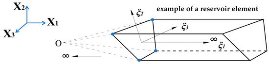
Figure 1.
Typical scale boundary finite element of fluid.
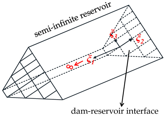
Figure 2.
Reservoir model discretized by SBFEM.
The basic equation and boundary conditions (Equations (1)–(4)) of the hydrodynamic pressure of reservoir in front of the dam are solved using the weighted residual method. Through the weight function w, the following weak integral equation (Equation (5)) can be obtained:
In order to derive the governing equations and boundary conditions of reservoir hydrodynamic pressure using SBFEM, it is necessary to transform the coordinates of the reservoir from the global Cartesian coordinate system to the local coordinate system of the scaled boundary. In the scaled boundary coordinate system, the radial local coordinate ξ1 has the range [0, +∞]. As shown in Figure 2, ξ1 = 0 is at the upstream face of the dam, and ξ1 = +∞ is at the infinity of the reservoir. The circumferential local coordinates ξ2 and ξ3 have the range [–1, 1]. The coordinates (X1, X2, X3) of the global Cartesian coordinate system at any point in the reservoir area can be expressed in terms of the local coordinates (ξ1, ξ2, ξ3) of the scaled boundary. The radial local coordinate ξ1 serves as a factor of proportionality, giving rise to the following set of equations:
where (x1, x2, x3) are the nodal coordinates of the elements on the interface between the reservoir and dam. represents the shape function of the elements, which is only related to the circumferential local coordinates but unrelated to the radial coordinate ξ1.
According to the transformation formula, the differential operator ▽ can be expressed in terms of the scaled boundary coordinates through the Jacobian matrix [J] as follows:
where [J]−1 = [{b1} {b2} {b3}].
By using the shape function for coordinate transformation, the hydrodynamic pressure at any point in an element can be expressed as
where {p(ξ1)} is the hydrodynamic pressure at nodes of the fluid element.
Equations (6)–(9) are introduced into the SBFEM hydrodynamic pressure integral Equation (5), and the partial integration is carried out. Finally, the governing equation (Equation (10)) and boundary conditions (Equation (11)) of hydrodynamic pressure can be obtained in the frequency domain as follows:
in which
where [N] denotes the interpolation shape function , and Γ in Equation (18) denotes the projection of the wet contour line of the reservoir at the interface between the dam and reservoir on the (X2, X3) plane.
It can be seen from Equations (12)–(19) that the coefficient matrices [E0], [E1], [E2], [C0], and [M1] are independent of the radial coordinate ξ1 and can be straightforwardly obtained from geometry information of the grid on the dam upstream face. Then the coefficient matrices of elements can be integrated into the total SBFEM coefficient matrices, the process of which is similar to the FEM.
In order to analytically solve the governing equation (Equation (10)), it is necessary to introduce the nodal force matrix of the hydrodynamic pressure.
Taking advantage of the new variables and expressions defined in Equation (21), the governing equation (Equation (10)) can be rewritten into a first-order ordinary differential equation (Equation (22)).
in which the coefficient matrix [Z] is the Hamilton matrix.
The eigenvalue problem, as shown in Equation (24), corresponding to the Hamilton matrix [Z] should be solved first.
in which [Λ] denotes the eigenvalue matrix, [Φ] denotes the eigenvector matrix, [λi] is the diagonal matrix, and the real part of λi is positive.
The inverse matrix of the matrix [Φ], which is denoted with [A], is solved and partitioned secondly.
In the end, by bringing in the boundary condition (Equation (11)) and carrying out a series of manipulations, the hydrodynamic pressure of the reservoir on the dam surface because of a seismic load can be expressed as
in which
From Equation (27) above, the hydrodynamic pressure consists of two components: the hydrodynamic pressure caused by the vibration of the dam upstream face {ün}, and that induced by the vibration of the river valley {ϋn} surrounding the reservoir area.
3. An Efficient Dynamic Coupling Calculation Method for Dam–Reservoir Systems
In Section 3.1, the conventional dynamic coupling method for dam and reservoir systems is described first, in which the hydrodynamic pressure is considered by means of the additional mass matrix [2,21,22,23]. In Section 3.2, the hydrodynamic pressure additional mass matrix, which is computed from Equation (27) as shown in Section 3.1, is further processed (in Section 3.2.2) according to the characteristics of the additional mass matrix as analyzed in Section 3.2.1. In Section 3.3, the efficient dynamic coupling calculation method based on the FEM-SBFEM is proposed with the hydrodynamic pressure additional mass matrix after treatment by way of Section 3.2.
3.1. Conventional Dynamic Coupling Analysis Method for Dam–Reservoir Systems
The FEM is employed for dam modeling, and the SBFEM is adopted for modeling the reservoir before the dam. The analysis equation for dynamic coupling of the dam and reservoir system is defined as follows:
in which [Ms], [Cs], and [Ks] are mass, damping, and stiffness matrices of the dam, respectively. {ür(t)}, and {ur(t)} are the relative acceleration, velocity, and displacement, respectively. {üg(t)} is the earthquake acceleration from the input system. [L1] is the conversion matrix for mapping global coordinates to the local coordinates of the dam upstream face.
After substituting Equation (27) into Equation (30), the dynamic coupling calculation equations are obtained as
where [Mu] and [Mv] are the dam upstream face and river valley components, respectively, of the hydrodynamic pressure additional mass matrix [Mp]. [L2] is the conversion matrix for mapping global coordinates to the local coordinates of the bank slope (river valley). As long as the additional mass matrix [Mp] is added to the mass matrix of the finite element dynamic equation of the dam, the hydrodynamic pressure due to the ground motion input in different directions can be considered.
3.2. Simplification of Hydrodynamic Pressure Additional Mass Matrix
3.2.1. Physical Meaning and Distribution Characteristics of Matrix
The calculated additional mass matrix [Mu] is a full matrix, and all elements are non-zero, that is, when calculating the hydrodynamic pressure caused by the excitation of the dam upstream face, the hydrodynamic pressure acting on a certain node is related to the acceleration excitations {ün} of all nodes on the dam upstream face below the water level. However, when calculating the hydrodynamic pressure caused by river valley excitation, the hydrodynamic pressure acting on a certain node on the dam upstream face is only related to the node acceleration excitations {ϋn} at the boundary between the dam surface and the river valley. Therefore, the additional mass matrix [Mv] is a very sparse matrix containing a large number of zero elements. Obviously, due to the existence of the additional mass matrix [Mu], the additional mass matrix [Mp] is a full matrix, which greatly increases the time consumption of solving the equivalent stiffness matrix in dynamic analysis.
From the above analysis, it can be seen that the node degree of freedom correlation of the additional mass matrix [Mp] can be reduced by the simplifying matrix [Mu]. When the additional mass matrix [Mu] is of order n (i.e., there are n nodes below the water level line on the dam upstream face in total); the physical meaning of the element is the hydrodynamic pressure acting on the node i caused by the unit normal acceleration excitation of the node j on the water upstream face. The i-th row elements in matrix [Mu], that is … … , are selected, and then these row elements give the contribution of all nodes on the upstream face of the dam (below the water level) to the hydrodynamic pressure acting on node i.
The distribution characteristics of the hydrodynamic pressure added mass matrix [Mu] are analyzed using the example of a vertical dam upstream face in a rectangular valley. The height of the dam is 200 m, and the width of the river valley is 400 m. The grid division of the reservoir is shown in Figure 3, and the water depth in front of the dam is 200 m (full reservoir).
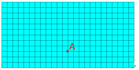
Figure 3.
Mesh of dam upstream face (A represents a node of the mesh).
After solving the added mass matrix of hydrodynamic pressure based on the SBFEM, the row elements corresponding to node A (see Figure 3) in the added mass matrix [Mu] are extracted, and the influence of all nodes at the dam upstream face on the hydrodynamic pressure of node A under unit normal acceleration excitation is shown in Figure 4 (normalized relative value). As shown in Figure 4, node A has the greatest impact on itself, and the closer the node is to node A, the greater the impact is on the hydrodynamic pressure of node A. Other nodes on the upstream face of the dam also conform to similar laws, so it is no longer described repetitively.
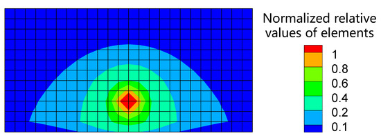
Figure 4.
Effect of all nodes on node A.
3.2.2. Theoretical Analysis and Simplified Processing Method
For the additional mass matrix [Mu], among all the elements in the i-th row, the element values corresponding to node i () and its adjacent nodes are relatively large, and the acceleration values of these closer nodes in the dynamic coupling analysis are not much different. Therefore, when calculating the hydrodynamic pressure acting on node i, the added mass element of the i-th row can be directly superimposed on , and the corresponding elements at the original position of the row are directly taken as 0, which means that the hydrodynamic pressure acting on node i is only related to the acceleration of node i, and it has nothing to do with the acceleration of other nodes on the dam upstream face. At the same time, the instantaneous acceleration distribution of the dam upstream face is not consistent, which contains both positive and negative values. Therefore, the above treatment method for the additional mass matrix will cause the amplification of hydrodynamic pressure. Considering the amplification effect of the superposition of additional mass elements on the hydrodynamic pressure, the appropriate reduction treatment is needed in the process of element superposition.
According to the physical meaning of each element of the additional mass matrix [Mu], a simple and easy simplification method is proposed by row processing, which is briefly described as follows:
(1) Extract the elements of the i-th row in the hydrodynamic pressure added mass matrix [Mu]. (2) Let the diagonal elements of the matrix , where α is the reduction coefficient (0 < α ≤ 1.0); at the same time, set the value of other non-diagonal elements to zero. (3) According to this method, the additional mass matrix [Mu] is processed from the first row until the last row.
After simplification, the additional mass matrix [Mu] is transformed into a new diagonal matrix [Muα]. The additional mass matrix [Mv] does not need to be simplified. Further, the overall additional mass matrix [Mp] is updated to [Mpα] as follows:
3.3. Efficient Dynamic Coupling Calculation Method Based on FEM-SBFEM
By replacing [Mp] with [Mpα] in Equation (31), the efficient dynamic coupling calculation method for dam–reservoir systems based on the FEM-SBFEM is established:
The simplification method only needs to provide a reduction coefficient α to realize the simplification of the additional mass matrix [Mp] to a large extent, which is simple and easy to implement. The processed additional mass matrix [Mpα] contains many zero elements, so the computational efficiency of dynamic coupling systems is greatly improved. The practice shows that the value of reduction coefficient α has an obvious influence on the calculation accuracy, which is presented in Section 4.
The efficient dynamic coupling calculation method based on the FEM-SBFEM is implemented on the strength of the Windows program GEODYNA [45], which was developed using object-oriented programming in Visual C++. Multicore parallel technology of the CPU is carried out in the GEODYNA software platform, by which the computational capacity of solving a large-scale nonlinear equation with millions of DOFs is enabled. The GEODYNA program has been widely used in the dynamic analysis of linear and nonlinear structures and fluid–solid coupling systems [2,21,22,23,46,47,48,49,50,51].
4. Dynamic Coupling Analysis of Arch Dam and Reservoir Systems
Based on the dynamic fluid–solid coupling analysis of a concrete arch dam and reservoir water under earthquake conditions, the sensitivity analysis for the value of reduction coefficient α is carried out. Different reduction factors α of additional mass matrix [Mpα] are selected to calculate and analyze the dynamic response of the arch dam. By comparing with the exact solution, which means the unsimplified full additional mass matrix [Mp] is utilized in dynamic analysis, the recommended value of reduction factor α is discussed.
4.1. Calculation Model
4.1.1. Dam and Reservoir Model
The Morrow Point arch dam [19,20,36] was selected to establish the finite element model, as shown in Figure 5. The concrete arch dam is 141.73 m high and simulated by 3D eight-node or degenerate isoparametric elements. The dam FEM model contains 15,000 elements, of which 2500 elements are on the upstream face of the arch dam. Assuming that the arch dam is located on a rigid bedrock, the bottom of the arch dam and the boundary in contact with the river valley are both constrained in X, Y, and Z directions. The construction joints of the arch dam are not taken into account in the FEM model.
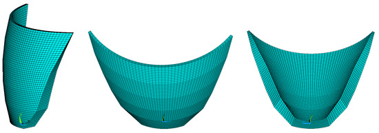
Figure 5.
FEM model of Morrow Point arch dam.
The water depth of the reservoir at the upstream side of the dam is 133.23 m. When the SBFEM is used to simulate the reservoir water in front of the dam in the dynamic coupling analysis, the 2D finite element mesh of the dam upstream face is immediately used to generate the prismatic semi-infinite reservoir water, as indicated in Figure 2. The grid of the dam already contains the reservoir water grid information, so there is no need to divide the reservoir water grid separately, which improves the pre-processing efficiency. There are 2350 grids below the water level on the upstream face of dam, which means that there are 2350 scaled boundary finite elements for the reservoir water.
4.1.2. Material Parameters, Input Seismic Load, and Damping Methods
The constitutive model employed for the concrete arch dam is a linear elastic model (density ρd = 2.4 g/cm3, elasticity modulus E = 25 GPa, Poisson’s ratio = 0.167), which can fully show the advanced nature of the proposed efficient dynamic coupling calculation method. The density ρw of the reservoir water is 1.0 g/cm3.
A set of earthquake waves, which were generated from the site spectrum of real engineering, were selected for dynamic analysis. As shown in Figure 6, the acceleration time history of three seismic waves was input from the bedrock with a consistent input method in up-downstream (X), vertical (Y), and dam axial (Z) directions. The peak ground acceleration (PGA) of horizontal bedrock motion, which is in the up-downstream and dam axial direction, was scaled to 1.5 m/s2, and the PGA of vertical bedrock motion was 1.0 m/s2.
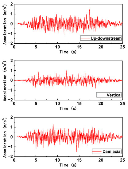
Figure 6.
Input bedrock motion.
The Rayleigh viscous damping method was adopted for the concrete arch dam in dynamic analysis [49]. A damping ratio of 5% was assumed for the concrete material.
4.2. Effect of Additional Mass Matrix Simplification
In the finite element model of the arch dam, there are 2397 nodes below the water level line on the dam upstream face, that is, there are 2397 node degrees of freedom in the semi-infinite reservoir water model. As a consequence, the unsimplified additional mass matrix [Mu] is a full matrix of order 2397, which contains 2397 × 2397 = 5,745,609 elements of the matrix and could provide an accurate dynamic coupling calculation result of dam and reservoir systems.
In the following numerical calculation and analysis, a total of 8 working conditions of hydrodynamic pressure additional mass matrix reduction coefficient α (0 < α ≤ 1.0) was selected for forming [Muα], in which α = 1.0, 0.9, 0.8, 0.7, 0.6, 0.5, 0.4, and 0.3. α = 1.0 indicates that the additional mass matrix is simplified to a diagonal matrix without reduction, and α ≈ 0 indicates that the added mass matrix [Muα] is close to the zero matrix, that is, the hydrodynamic pressure is almost not considered. When 0 < α ≤ 1.0 in this numerical case, the simplified added mass matrix [Muα] is a diagonal matrix, which contains only 2397 elements and can present an approximate analysis result of the dynamic interaction of the dam and reservoir. The simplification of the additional mass matrix can not only save a lot of memory occupied by the additional mass matrix of hydrodynamic pressure but also greatly reduce the computational time. However, only a reasonable value of the reduction coefficient α can ensure high calculation accuracy, as discussed below.
4.3. Results and Discussion
Under different reduction coefficient (α = 1.0, 0.9, 0.8, 0.7, 0.6, 0.5, 0.4, and 0.3) conditions, the effects of the hydrodynamic pressure added mass matrix [Muα] ([Mpα]) on the dynamic stress and acceleration extreme (maximum) value of the arch dam and their regularities of distribution and calculation time are studied. When calculating the error of dynamic stress and acceleration of the arch dam caused by the simplification of the additional mass matrix, the accurate calculation results of the unsimplified additional mass matrix [Mu] ([Mp]) are taken as the benchmark. The results of the unsimplified additional mass matrix were verified to be of high accuracy [2,21]. By comparing the calculation accuracy and calculation time, the recommended value of the reduction coefficient α is given.
4.3.1. Acceleration of Arch Dam
Table 1 summarizes the maximum absolute values of the arch dam acceleration in up-downstream (ax) and vertical (ay) directions under different reduction coefficients α for simplification of additional mass matrix and unsimplified additional mass matrix conditions when the earthquake occurs. Table 2 shows the errors corresponding to the maximum dynamic acceleration caused by simplification of the added mass matrix of hydrodynamic pressure. It can be concluded from Table 1 and Table 2 that the additional mass matrix reduction coefficient α has a big impact on the acceleration in the up-downstream direction (ax) but has relatively little impact on the vertical acceleration (ay). Compared with the accurate results in the condition of the unsimplified additional mass matrix, the maximum errors of acceleration, when the reduction coefficient α = 0.6 and 0.7, are 0.4% and 4.6%, respectively, which are acceptable from the perspective of calculation accuracy since the max errors are limited to less than 5.0%. When the reduction coefficient α < 0.6 and α > 0.7, the max errors of acceleration become bigger, which are from 9.0% to 22.7%.

Table 1.
Max dynamic acceleration of arch dam.
Table 2.
Error of max dynamic acceleration of arch dam.
Figure 7 plots the distribution of the maximum absolute acceleration along the up-downstream direction (ax) on the upstream face of the arch dam. As shown in Figure 7, the distribution laws of the maximum acceleration along the up-downstream direction (ax) for each condition are similar, but the extent and area of the high acceleration response region are significantly different and gradually change with the decrease of the reduction coefficient α. In addition, the maximum acceleration distribution is most consistent with the accurate analysis solution (from unsimplified additional mass matrix) when the reduction coefficient α = 0.6, which also corresponds to the minimum error of acceleration in both vertical (ay) and up-downstream (ax) directions, as summarized in Table 2.
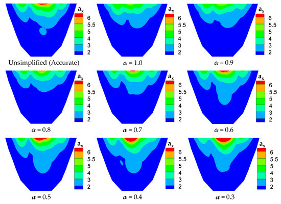
Figure 7.
Distribution of maximum acceleration along the up-downstream direction (ax) on upstream face of arch dam (m/s2).
4.3.2. Stress of Arch Dam
Under different hydrodynamic pressure added mass matrix conditions, the maximum dynamic stresses of the arch dam concrete, including major principal stress (σ1) and minor principal stress (σ3), that occurred during the earthquake are collected in Table 3. The compressive stress of the dam concrete is set to be positive. Table 4 lists the errors corresponding to the maximum dynamic stress when the added mass matrix of hydrodynamic pressure is simplified with different reduction coefficients α. Table 3 and Table 4 demonstrate that the reduction coefficient α has an obvious influence on both the major principal stress and minor principal stress of arch dam. As shown in Table 4, the maximum errors of dynamic stress are less than 5.0% when the reduction coefficient α = 0.4, 0.6, 0.7, and 0.8, which means the calculation accuracy of dynamic stress is effectively controlled. Furthermore, the maximum errors of dynamic stress are 2.2% and 1.3%, respectively, for reduction coefficient α = 0.6 and 0.8, the errors of which are relatively small in all reduction coefficients conditions. The maximum errors of dynamic stress vary from 5.0 to 11.2%, when the reduction coefficient α = 0.3, 0.5, 0.9, and 1.0, which are relatively big.
Table 3.
Max dynamic stress of arch dam.
Table 4.
Error of max dynamic stress of arch dam.
The distribution of the maximum dynamic minor principal stress (σ3) on the upstream face of the arch dam for every condition of hydrodynamic pressure added mass matrix is depicted in Figure 8. Because seismic loads on the dam will eventually be transferred to the arch abutment, there are high maximum minor principal stress values on the contour of the dam, as shown in Figure 8. As seen in Figure 8, the dynamic minor principal stress (σ3) distribution rules of each condition are basically consistent, whereas there are some differences in the location and range of the high stress zone of the arch dam. Although the calculation accuracy of the maximum dynamic stress is relatively high for the reduction coefficient α = 0.8, as mentioned above, the scope and area of the high stress zone are obviously different from the accurate solution for the unsimplified added mass matrix. For the condition of the reduction coefficient α = 0.4, the calculation error of maximum dynamic stress is restricted to less than 5%; however, the position of the high stress zone distinctly has a certain degree of deviation compared to the accurate result. When the reduction coefficient α = 0.6, the distribution law of the maximum dynamic stress of the arch dam, including the location of the high stress zone and the range of the high stress zone, is the most similar to the accurate solution, and the computational accuracy for maximum dynamic stress is also high in all the simplification conditions of the additional mass matrix reduction coefficient α, as seen in Table 4.
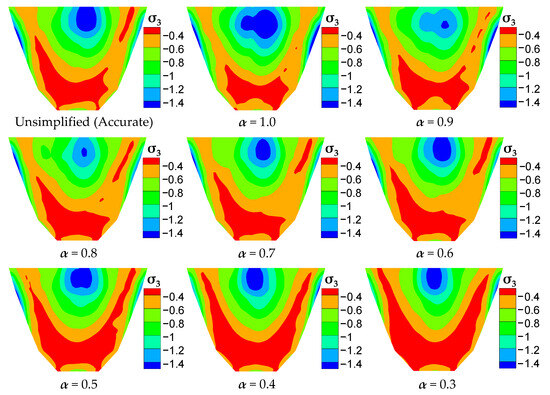
Figure 8.
Distribution of maximum minor principal stress (σ3) on upstream face of arch dam (MPa).
4.3.3. Computational Efficiency
The CPU model of the desktop computer used in the numerical calculation is an Intel (R) Xeon (R) Gold 6248R, whose main frequency is 3.00 Hz. Table 5 shows the consumption time and the corresponding time-consuming ratio of the dynamic fluid–solid coupling calculation for the dam–reservoir systems under different hydrodynamic pressure added mass matrix conditions. When calculating the time-consuming ratio of different working conditions, the accurate solution using the unsimplified additional mass matrix is used as the benchmark, of which the time-consuming ratio is 100%.
Table 5.
Consumption time and the corresponding time-consuming ratio.
It can be seen from Table 5 that the consumption time of calculation is the most (117.799 h) when the unsimplified hydrodynamic pressure added mass matrix is used, which means there are accurate results of the dam dynamic response. When different reduction coefficients α are used to simplify the additional mass matrix, the consumption time of the dynamic coupling calculation is basically the same, which accounts for about 5% of that under the accurate solution condition. Table 5 shows that for the proposed efficient dynamic coupling calculation method of dam–reservoir systems, the elapsed time is sharply reduced, and the calculation efficiency has made a great jump. It can be seen that the additional mass matrix has a great influence on the computational efficiency of dynamic coupling analysis. Combining Table 2, Table 4, and Table 5, it can be seen that the dynamic coupling calculation efficiency of dam–reservoir systems has been greatly improved after the additional mass matrix is simplified, and the reasonable selection of reduction coefficient α can effectively ensure high calculation accuracy.
4.3.4. Suggested Value of Reduction Coefficient α
According to the analysis of the dam acceleration response results, when the reduction coefficient is 0.6, the calculation accuracy of the maximum acceleration of the dam is the highest (Table 2), and the distribution law of the maximum acceleration of the dam at this time is most similar to the accurate solution (Figure 7). In addition, by comprehensively analyzing the results of the maximum dynamic stress of the dam (Table 4) and its distribution law (Figure 8), it can be known that the reduction coefficient α of 0.6 cannot only ensure the accuracy of the distribution law of the maximum dynamic stress of the dam but also the high calculation accuracy of the maximum dynamic stress. At the same time, from the perspective of computational efficiency, different reduction coefficients almost do not affect the running time of the coupling calculation, and the calculation time can be reduced to about one-twentieth of the unsimplified condition of the additional mass matrix.
In summary, the suggested value of the reduction coefficient is 0.6, which can control the error of coupling calculation results of the dynamic response of the dam within 5% and reduce the elapsed calculation time by more than one order of magnitude. By simplifying the added mass matrix of hydrodynamic pressure, the proposed efficient analysis method can greatly reduce the calculation consumption time and improve the calculation efficiency under the premise of ensuring good accuracy. The efficient method proposed in this study can realize the simplified and efficient calculation and analysis of dynamic fluid–solid coupling between the dam and reservoir under earthquake conditions and is more suitable for engineering calculations with large degrees of freedom than traditional methods.
5. Conclusions
In this study, the hydrodynamic pressure of a reservoir with semi-infinite 3D shapes is directly solved using the SBFEM in 2D, which acting on the dam upstream face is expressed in the form of an additional mass matrix. Further, the dynamic coupling analysis method of dam–reservoir systems, in which the dam is simulated using the FEM, under earthquake conditions, is improved by processing the additional mass matrix of hydrodynamic pressure. Furthermore, the computational efficiency and accuracy of the improved analysis method are studied and verified with the seismic calculation of arch dam–reservoir systems. The following major conclusions are drawn:
- An efficient 3D dynamic fluid–solid coupling calculation method for dam–reservoir systems based on the FEM-SBFEM is proposed by simplifying the hydrodynamic pressure additional mass matrix according to the physical meaning and distribution characteristics of the additional matrix. The proposed method not only ensures the high accuracy of the numerical calculation results but also greatly reduces the consumption time of the dynamic coupling calculation.
- The hydrodynamic pressure added mass matrix has a great influence on the computational efficiency of dynamic coupling analysis. The proposed method, which is simple and easy to implement, only needs to determine a reduction coefficient α (0 < α ≤ 1.0) to simplify the hydrodynamic pressure added mass matrix to a great extent and save a lot of memory occupied by the added mass matrix.
- The suggested value of the reduction coefficient α for the added mass matrix of the hydrodynamic pressure is selected to be 0.6 so as to ensure that the distribution law of the dynamic response of the dam is consistent with the accurate solution, which means the unsimplified additional mass matrix condition. The error of the maximum value of the dynamic response of the dam is limited to within 5%, which is acceptable, and the elapsed time of calculation can be reduced to one twentieth of the accurate solution, which is a great jump in calculation efficiency.
- The proposed method provides an accurate and efficient approach for dynamic fluid–solid coupling analysis and seismic safety evaluation of dam and reservoir systems and makes the application of dam–reservoir systems and a fluid–solid coupling analysis method in fine analysis with large-scale DOFs technically feasible.
- The proposed dynamic coupling calculation method can also be further applied to the nonlinear numerical analysis of CFRD and the fine damage analysis of concrete dams under earthquake conditions. Furthermore, the additional mass matrix simplification method in the dynamic coupling analysis of dam and reservoir systems provided in this study is also applicable to the additional mass of hydrodynamic pressure calculated by other numerical methods (FEM, BEM, PSBFEM, etc.).
Author Contributions
Conceptualization, H.X. and D.Z.; methodology, H.X. and J.X.; software, H.X. and K.C.; validation, H.X. and D.Y.; resources, H.X., K.C., and D.Z.; writing—original draft preparation, H.X. and J.X.; writing—review and editing, D.Y. and K.C.; supervision, J.X., H.X, D.Y., K.C., and D.Z. All authors have read and agreed to the published version of the manuscript.
Funding
This research was supported by the Project funded by the China Postdoctoral Science Foundation (2021M690998), the National Natural Science Foundation of China (Grant Nos. 52192674, U2240211), and the Doctoral Research Start-up Fund Program Project (2021-BS-065).
Data Availability Statement
Data are not publicly available due to data privacy reasons.
Conflicts of Interest
The authors declare no conflict of interest.
References
- Song, C.; Wolf, J.P. The scaled boundary finite-element method—Alias consistent infinitesimal finite-element cell method—For elastodynamics. Comput. Methods Appl. Mech. Eng. 1997, 147, 329–355. [Google Scholar] [CrossRef]
- Xu, J.; Xu, H.; Yan, D.; Chen, K.; Zou, D. A Novel Calculation Method of Hydrodynamic Pressure Based on Polyhedron SBFEM and Its Application in Nonlinear Cross-Scale CFRD-Reservoir Systems. Water 2022, 14, 867. [Google Scholar] [CrossRef]
- Zhang, G.; Zhao, M.; Zhang, J.; Du, X. Scaled Boundary Perfectly Matched Layer (SBPML): A novel 3D time-domain artificial boundary method for wave problem in general-shaped and heterogeneous infinite domain. Comput. Methods Appl. Mech. Eng. 2023, 403, 115738. [Google Scholar] [CrossRef]
- Zhang, P.; Du, C.; Zhao, W.; Zhang, D. Hydraulic fracture simulation of concrete using the SBFEM-FVM model. Struct. Eng. Mech. 2021, 80, 553–562. [Google Scholar]
- Li, J.; Shi, Z.; Liu, L.; Song, C. An efficient scaled boundary finite element method for transient vibro-acoustic analysis of plates and shells. Comput. Struct. 2020, 231, 106211. [Google Scholar] [CrossRef]
- Fouladi, M.Q.; Badiei, P.; Vahdani, S. A study on full interaction of water waves with moored rectangular floating breakwater by applying 2DV scaled boundary finite element method. Ocean Eng. 2021, 220, 108450. [Google Scholar] [CrossRef]
- Wang, P.; Lu, R.; Yan, Q.; Bao, X.; Zhang, J.; Liu, L. The internal substructure method for shock wave input in 2D fluid-structure interaction analysis with unbounded domain using doubly-asymptotic ABC. Mech. Adv. Mater. Struct. 2023, 30, 3111–3124. [Google Scholar] [CrossRef]
- Pfeil, S.; Gravenkamp, H.; Duvigneau, F.; Woschke, E. Scaled boundary finite element method for hydrodynamic bearings in rotordynamic simulations. Int. J. Mech. Sci. 2021, 199, 106427. [Google Scholar] [CrossRef]
- Zhao, M.; Wang, X.; Wang, P.; Du, X.; Liu, J. Seismic water-structure interaction analysis using a modified SBFEM and FEM coupling in a frequency domain. Ocean Eng. 2019, 189, 106374. [Google Scholar] [CrossRef]
- Deeks, A.J.; Cheng, L. Potential flow around obstacles using the scaled boundary finite-element method. Int. J. Numer. Methods Fluids 2003, 41, 721–741. [Google Scholar] [CrossRef]
- Li, B.; Cheng, L.; Deeks, A.J.; Teng, B. A modified scaled boundary finite-element method for problems with parallel side-faces. Part II. Application and evaluation. Appl. Ocean Res. 2005, 27, 224–234. [Google Scholar] [CrossRef]
- Li, B.; Cheng, L.; Deeks, A.J.; Zhao, M. A semi-analytical solution method for two-dimensional Helmholtz equation. Appl. Ocean Res. 2006, 28, 193–207. [Google Scholar] [CrossRef]
- Teng, B.; Zhao, M.; He, G.H. Scaled boundary finite element analysis of the water sloshing in 2D containers. Int. J. Numer. Methods Fluids 2006, 52, 659–678. [Google Scholar] [CrossRef]
- Cao, F.S.; Teng, B. Scaled boundary finite element analysis of wave passing a submerged breakwater. China Ocean Eng. 2008, 22, 241–251. [Google Scholar]
- Song, H.; Tao, L. Hydroelastic response of a circular plate in waves using scaled boundary FEM. In Proceedings of the ASME 2009 28th International Conference on Ocean, Offshore and Arctic Engineering, Honolulu, HI, USA, 31 May–5 June 2009. [Google Scholar]
- Song, H.; Tao, L. Semi-analytical solution of Poisson’s equation in bounded domain. ANZIAM J. 2009, 51, C169–C185. [Google Scholar] [CrossRef]
- Song, H.; Tao, L. An efficient scaled boundary FEM model for wave interaction with a nonuniform porous cylinder. Int. J. Numer. Methods Fluids 2010, 63, 96–118. [Google Scholar] [CrossRef]
- Liu, J.; Lin, G.; Li, J. Short-crested waves interaction with a concentric cylindrical structure with double-layered perforated walls. Ocean Eng. 2012, 40, 76–90. [Google Scholar] [CrossRef]
- Lin, G.; Du, J.; Hu, Z. Dynamic dam-reservoir interaction analysis including effect of reservoir boundary absorption. Sci. China Ser. E Technol. Sci. 2007, 50, 1–10. [Google Scholar] [CrossRef]
- Lin, G.; Wang, Y.; Hu, Z. An efficient approach for frequency-domain and time-domain hydrodynamic analysis of dam-reservoir systems. Earthq. Eng. Struct. Dyn. 2012, 41, 1725–1749. [Google Scholar] [CrossRef]
- Xu, H.; Zou, D.; Kong, X.; Hu, Z. Study on the effects of hydrodynamic pressure on the dynamic stresses in slabs of high CFRD based on the scaled boundary finite-element method. Soil Dyn. Earthq. Eng. 2016, 88, 223–236. [Google Scholar] [CrossRef]
- Xu, H.; Zou, D.; Kong, X.; Su, X. Error study of Westergaard’s approximation in seismic analysis of high concrete-faced rockfill dams based on SBFEM. Soil Dyn. Earthq. Eng. 2017, 94, 88–91. [Google Scholar] [CrossRef]
- Xu, H.; Zou, D.; Kong, X.; Hu, Z.; Su, X. A nonlinear analysis of dynamic interactions of CFRD-compressible reservoir system based on FEM-SBFEM. Soil Dyn. Earthq. Eng. 2018, 112, 24–34. [Google Scholar] [CrossRef]
- Wang, X.; Jin, F.; Prempramote, S.; Song, C. Time-domain analysis of gravity dam–reservoir interaction using high-order doubly asymptotic open boundary. Comput. Struct. 2011, 89, 668–680. [Google Scholar] [CrossRef]
- Gao, Y.; Jin, F.; Wang, X.; Wang, J. Finite Element Analysis of Dam–Reservoir Interaction Using High-Order Doubly Asymptotic Open Boundary. In Seismic Safety Evaluation of Concrete Dams; Butterworth-Heinemann: Oxford, UK, 2013; pp. 173–198. [Google Scholar]
- Das, S.K.; Mandal, K.K.; Niyogi, A.G. Finite element-based direct coupling approach for dynamic analysis of dam–reservoir system. Innov. Infrastruct. Solut. 2023, 8, 44. [Google Scholar] [CrossRef]
- Gorai, S.; Maity, D. Seismic Performance Evaluation of Concrete Gravity Dams in Finite-Element Framework. Pract. Period. Struct. Des. Constr. 2022, 27, 04021072. [Google Scholar] [CrossRef]
- Wang, C.; Zhang, H.; Zhang, Y.; Guo, L.; Wang, Y.; Thira Htun, T.T. Influences on the seismic response of a gravity dam with different foundation and reservoir modeling assumptions. Water 2021, 13, 3072. [Google Scholar] [CrossRef]
- Pelecanos, L.; Kontoe, S.; Zdravković, L. The effects of dam–reservoir interaction on the nonlinear seismic response of earth dams. J. Earthq. Eng. 2020, 24, 1034–1056. [Google Scholar] [CrossRef]
- Sharma, V.; Fujisawa, K.; Murakami, A. Space–time FEM with block-iterative algorithm for nonlinear dynamic fracture analysis of concrete gravity dam. Soil Dyn. Earthq. Eng. 2020, 131, 105995. [Google Scholar] [CrossRef]
- Karabulut, M.; Kartal, M.E. Seismic analysis of Roller Compacted Concrete (RCC) dams considering effect of viscous boundary conditions. Comput. Concr. Int. J. 2019, 27, 255–266. [Google Scholar]
- Wang, J.T.; Lv, D.D.; Jin, F.; Zhang, C.H. Earthquake damage analysis of arch dams considering dam–water–foundation interaction. Soil Dyn. Earthq. Eng. 2013, 49, 64–74. [Google Scholar] [CrossRef]
- Bayraktar, A.; Kartal, M.E. Linear and nonlinear response of concrete slab on CFR dam during earthquake. Soil Dyn. Earthq. Eng. 2010, 30, 990–1003. [Google Scholar] [CrossRef]
- Wang, J.T.; Chopra, A.K. Linear analysis of concrete arch dams including dam-water-foundation rock interaction considering spatially varying ground motions. Earthq. Eng. Struct. Dyn. 2010, 39, 731–750. [Google Scholar] [CrossRef]
- Bayraktar, A.; Dumanoǧlu, A.A.; Calayir, Y. Asynchronous dynamic analysis of dam-reservoir-foundation systems by the Lagrangian approach. Comput. Struct. 1996, 58, 925–935. [Google Scholar] [CrossRef]
- Fok, K.L.; Chopra, A.K. Earthquake analysis of arch dams including dam–water interaction, reservoir boundary absorption and foundation flexibility. Earthq. Eng. Struct. Dyn. 1986, 14, 155–184. [Google Scholar] [CrossRef]
- Fenves, G.; Chopra, A.K. Earthquake analysis of concrete gravity dams including reservoir bottom absorption and dam-water-foundation rock interaction. Earthq. Eng. Struct. Dyn. 1984, 12, 663–680. [Google Scholar] [CrossRef]
- Bouaanani, N.; Miquel, B. An error estimator for transmitting boundary conditions in fluid-structure interaction problems. WIT Trans. Built Environ. 2011, 115, 169–178. [Google Scholar]
- Küçükarslan, S.; Coşkun, S.B. Transient dynamic analysis of dam-reservoir interaction by coupling DRBEM and FEM. Eng. Comput. 2004, 21, 692–707. [Google Scholar] [CrossRef]
- Fahjan, Y.M.; Börekçi, O.S.; Erdik, M. Earthquake-induced hydrodynamic pressures on a 3D rigid dam–reservoir system using DRBEM and a radiation matrix. Int. J. Numer. Methods Eng. 2003, 56, 1511–1532. [Google Scholar] [CrossRef]
- Tsai, C.S.; Lee, G.C.; Yeh, C.S. Time-domain analyses of three-dimensional dam-reservoir interactions by BEM and semi-analytical method. Eng. Anal. Bound. Elem. 1992, 10, 107–118. [Google Scholar] [CrossRef]
- Tsai, C.S. Analyses of three-dimensional dam—Reservoir interactions based on bem with particular integrals and semi-analytical solution. Comput. Struct. 1992, 43, 863–872. [Google Scholar] [CrossRef]
- Tsai, C.S.; Lee, G.C. Arch dam–fluid interactions: By FEM–BEM and substructure concept. Int. J. Numer. Methods Eng. 1987, 24, 2367–2388. [Google Scholar] [CrossRef]
- Degao, Z.; Xianjing, K.; Bin, X. User Manual for Geotechnical Dynamic Nonlinear Analysis; Institute of Earthquake Engineering, Dalian University of Technology: Dalian, China, 2005. [Google Scholar]
- Dassault Systemes Simulia Corp. ABAQUS Analysis User’s Guide. 2016. Available online: http://130.149.89.49:2080/v2016/books/usb/default.htm?startat=pt04ch18s01aus106.html (accessed on 24 August 2023).
- Chen, K.; Zou, D.; Tang, H.; Liu, J.; Zhuo, Y. Scaled boundary polygon formula for Cosserat continuum and its verification. Eng. Anal. Bound. Elem. 2021, 126, 136–150. [Google Scholar] [CrossRef]
- Qu, Y.; Zou, D.; Kong, X.; Yu, X.; Chen, K. Seismic cracking evolution for anti-seepage face slabs in concrete faced rockfill dams based on cohesive zone model in explicit SBFEM-FEM frame. Soil Dyn. Earthq. Eng. 2020, 133, 106106. [Google Scholar] [CrossRef]
- Pang, R.; Xu, B.; Zhou, Y.; Song, L. Seismic time-history response and system reliability analysis of slopes considering uncertainty of multi-parameters and earthquake excitations. Comput. Geotech. 2021, 136, 104245. [Google Scholar] [CrossRef]
- Zou, D.; Xu, B.; Kong, X.; Liu, H.; Zhou, Y. Numerical simulation of the seismic response of the Zipingpu concrete face rockfill dam during the Wenchuan earthquake based on a generalized plasticity model. Comput. Geotech. 2013, 49, 111–122. [Google Scholar] [CrossRef]
- Chen, K.; Zou, D.; Liu, J.; Zhuo, Y. A high-precision formula for mixed-order polygon elements based on SBFEM. Comput. Geotech. 2023, 155, 105209. [Google Scholar] [CrossRef]
- Nie, X.; Chen, K.; Zou, D.; Kong, X.; Liu, J.; Qu, Y. Slope stability analysis based on SBFEM and multistage polytree-based refinement algorithms. Comput. Geotech. 2022, 149, 104861. [Google Scholar] [CrossRef]
Disclaimer/Publisher’s Note: The statements, opinions and data contained in all publications are solely those of the individual author(s) and contributor(s) and not of MDPI and/or the editor(s). MDPI and/or the editor(s) disclaim responsibility for any injury to people or property resulting from any ideas, methods, instructions or products referred to in the content. |
© 2023 by the authors. Licensee MDPI, Basel, Switzerland. This article is an open access article distributed under the terms and conditions of the Creative Commons Attribution (CC BY) license (https://creativecommons.org/licenses/by/4.0/).