Article

Two-Leak Isolation in Water Distribution Networks Based on k-NN and Linear Discriminant Classifiers

by
Carlos Andrés Rodríguez-Argote
1,
Ofelia Begovich-Mendoza
1,
Adrián Navarro-Díaz
2,
Ildeberto Santos-Ruiz
3,
Vicenç Puig
4 and
Jorge Alejandro Delgado-Aguiñaga
5,*
1
Centro de Investigación y de Estudios Avanzados, Cinvestav Guadalajara, Av. del Bosque 1145, El Bajío, Zapopan 45019, Mexico
2
Tecnologico de Monterrey, School of Engineering and Sciences, Av. General Ramón Corona 2514, Zapopan 45138, Mexico
3
Tecnológico Nacional de México, I. T. Tuxtla Gutiérrez, TURIX-Dynamics Diagnosis and Control Group, Carretera Panamericana S/N, Tuxtla Gutiérrez 29050, Mexico
4
Institut de Robòtica i Informàtica Industrial, Universitat Politècnica de Catalunya, CSIC-UPC, Parc Tecnològic de Barcelona, C Llorens i Artigas 4-6, 08028 Barcelona, Spain
5
Centro de Investigación, Innovación y Desarrollo Tecnológico, CIIDETEC-UVM, Universidad del Valle de México, Tlaquepaque 45604, Mexico
*
Author to whom correspondence should be addressed.
Water 2023, 15(17), 3090; https://doi.org/10.3390/w15173090
Submission received: 30 June 2023 / Revised: 12 August 2023 / Accepted: 16 August 2023 / Published: 29 August 2023

Abstract

:
In this paper, the two-simultaneous-leak isolation problem in water distribution networks is addressed. This methodology relies on optimal sensor placement together with a leak location strategy using two well-known classifiers: k-NN and discriminant analysis. First, zone segmentation of the water distribution network is proposed, aiming to reduce the computational cost that involves all possible combinations of two-leak scenarios. Each zone is composed of at least two consecutive nodes, which means that the number of zones is at most half the number of nodes. With this segmentation, the leak identification task is to locate the zones where the pair of leaks are occurring. To quantify the uncertainty degree, a relaxation node criterion is used. The simulation results evidenced that the outcomes are accurate in most cases by using one-relaxation-node and two-relaxation-node criteria.

1. Introduction

In recent years, the water cycle has been unbalanced due to climate change. Moreover, exponential growth of the population and drought have caused overuse of natural water resources such that both superficial and underground water are more scarce. In this context, water management companies have experienced severe complications to supply the water demand, especially in the low-water-level season. According to a recent study carried out by OECD [1], water losses in water distribution networks (WDN) in the worst cases reaches up to 65% due to leaks, which can be caused by the natural aging of pipes, earthquakes, illegal intrusion, poor quality of the pipe material, temperature and pressure, non-use of standard pipe laying methods, geological changes and human damage, among others [2,3]. Moreover, health problems and social conflicts are part of this complex problem affecting governments worldwide.
As mentioned above, the mismanagement of drinking water in networks is considered a global crisis. For this reason, continuous monitoring of the WDN has became increasingly important since quick leak detection allows timely repair, which, in turn, reduces the water loss. In this sense, several leak diagnosis techniques have been proposed by the scientific community. For instance, fault-sensitive-based, model-based and transient-based techniques have been reported considering either single- or multi-leak problems [4,5,6,7,8,9] for both single and branched pipelines. Moreover, to address the leak diagnosis problem in a WDN, these techniques are not generally suitable and other strategies have also been proposed, but they are based on artificial intelligence (AI) and data-driven approaches, as in [10,11,12,13,14], to mention a few recent works. Other approaches that have been used for a long time, such as the acoustic-based approach, identify the area where the leak is occurring on the basis of changes in the noise generated by measurements coming from the WDN [15,16,17].
On the other hand, in [18], the authors proposed a model-based methodology on the basis of a sensitivity analysis using residuals. These residuals are used to estimate the leaky node. This methodology is applied when certain thresholds previously established using the historical demand in the network are exceeded. This methodology has been tested in real-life scenarios with acceptable results [19,20]; however, the dependence on a well-calibrated model of the WDN is highlighted. Following this direction, several strategies for control, supervision and diagnosis of pipes have been proposed to reduce the effects produced by network leaks [11]. These strategies include methodologies for modeling WDN using software, optimal sensor placement as well as data validation and reconstruction of sensors and several continuous monitoring techniques of the network for hydraulic and water quality analysis.
In addition, artificial intelligence methods have been used to solve many problems, including leak diagnosis. In [14], the authors propose a portable application using artificial intelligence (AI) for the automatic detection of changes in the characteristic noise of water in the network pipelines of the network to detect leaks. However, this methodology requires human resources that actively perform measurements throughout the network, or equipment that generally has a high economic cost. Similarly, data-driven methodologies have been developed to rely less on hydraulic models. On the one hand, the use of classifiers such as those based on k-NN, Bayesian and discriminant analysis methods have been explored in [21,22,23,24]. In [25], a statistical classifier with a finite impulse response (FIR) filter, which was added to improve the classification results, is presented. Following this direction, a comparison between the use of residuals with cosine distances to train a variety of classifiers is shown in [26]. Other data-driven methodologies that have been developed are based on artificial neural and convolutional neural networks [27,28,29,30], which, in turn, have been improved by applying deep learning [31,32,33]. In [32], the use of a graph-based neural network for leak detection and location is proposed instead of using data.
In most of the above-mentioned studies, as well as in those of other groups, the issues of leak diagnosis in WDN have focused on the single-leak problem, leaving aside the multiple-leak problem. Nonetheless, several studies have addressed this complex problem, such as [12], which proposes a methodology to isolate multiple leaks caused by seismic damage using genetic algorithms, and, similarly, in [13], a methodology based on data analysis is proposed for the detection and isolation of possible leaks, employing a radial base function (RBF) interpolation technique. In practice, a realistic issue is the case of multiple leaks, and, since the extension from a single-leak case to a multiple-leak case brings new scientific challenges, the main objective of the present work is to develop a new methodology based on machine learning classifiers to address this multi-leak problem in WDN as an extension of former studies for the single-leak case.
This paper is organized as follows: Section 2 presents the sensor placement strategy, and the leak isolation strategy is described in detail to confront the two-simultaneous-leak problem in WDN on the basis of two different classifiers: k-NN and discriminant analysis. Section 2.2 describes several leak cases to illustrate the performance of the leak location strategy, and the results are described in detail. Lastly, in Section 4, conclusions and future perspectives are discussed.

2. Materials and Methods

From a general point of view, the leak isolation problem in water distribution networks is addressed by performing two essential steps: optimal sensor placement and leak location. Usually, a reduced number of sensors are available and they must be placed in a way that most leaks can be isolated with accuracy.
In practice, the instrumentation of a WDN is not easy to perform. On the one hand, the accessibility is a constraint since pipes are often buried, and, on the other hand, the cost of devices is high. The philosophy of the isolation algorithms is to locate leaks as accurately as possible by using the least amount of sensors considering that an increased number of sensors does not imply an improved performance of a leak isolation methodology.
Since our proposal is mainly focused on the development of a leak isolation methodology, and good sensor placement is important to improve results, we use a previously established sensor placement methodology that has proven to provide reliable results. The sensor placement methodology used in this work is based on the net coverage calculation approach proposed in [34]. This method involves the use of residuals to assess the effectiveness of a candidate sensor placement in detecting leaks in all nodes.
On the other hand, to diagnose two simultaneous leaks, the proposed methodology is based on the use of classifiers. Particularly, the performances of a k-NN-based classifier and a discriminant-analysis-based classifier are compared. It should be noted that this leak problem is complex since it is a combinatorial problem in itself. To address this situation, a zone-based analysis of the WDN is proposed. To make the leak isolation more reliable, the leak location task is performed over an extended period of time using recursivity. Both the sensor placement methodology and the leak location methodology are summarized hereinafter.

2.1. Sensor Placement

The sensor placement methodology is based on the leak location using the correlation between pressure measurements in the presence of a leak and all possible leak scenarios (one at each node), as presented in [34]. For a network with n nodes and N s sensors, a residual vector r is obtained as follows:
r = p 1 p ^ 1 p 2 p ^ 2 p N s p ^ N s
where each element is computed as the difference between the pressure measurements (in the presence of leak) p i , and the estimated pressure in a scenario without leak p ^ i . Note that there is an element of the residual vector for every available measurement on the network. Here, the number of sensors N s is chosen considering the following criteria: sensor availability, physical constraints limiting accessibility to certain areas of the network and feasibility, which means that the installation of a large number of sensors does not necessarily mean an improvement in the leak diagnosis performance, as discussed in [34,35]. To correlate the residuals, a sensitivity matrix must be obtained to determine the possible effects of the various leakage scenarios on the pressure measurements. The sensitivity matrix is then defined as follows:
s = p 1 f 1 p ^ 1 f 1 p 1 f n p ^ 1 f n p N s f 1 p ^ N s f 1 p N s f n p ^ N s f n
where p i f j is the pressure measured on the node i under the presence of the leak f j in the node j, p ^ i is the pressure measured on the node i on the free-leak scenario and f j is the leakage flow at the node j. Note that, for the estimation of the sensitivities, n possible leaks locations were used, one per each node, and the leakage flow rate f j used for the sensitivity calculation may be different from the leak flow presented in the residuals computation.
Once the residuals and sensitivities have been obtained, the following step is to estimate the correlation between the residual vector with each column of the sensitivity matrix; this is completed using normalized projection between the residual and column j defined as
ψ j = r T s j r s j
where r is the residual vector and s j is the column j of the sensitivity matrix s. So, as result of obtaining all the possible correlations, a vector ψ = [ ψ 1 ψ 2 ψ n ] , which indicates the correlation of the flow rate with each of the n nodes of the network so that the candidate node k presenting the leak is the element with the highest correlation
ψ k = max ( ψ 1 , , ψ n )
Using the above procedure, the sensor placement methodology is developed; initially, it will be considered that the pressure of all the nodes that make up the network are monitored and that a leakage scenario is simulated in each of the nodes to obtain n residuals, so that, using Equations (1) and (2), the residual matrix and the sensitivity matrix are obtained.
R = r 1 r 2 r n
S = S 1 S 2 S n
The next step is to calculate a binary matrix L of all the possible combinations of sensor placements for N s sensors in a network consisting of n nodes, which is defined as
L = L 1 L 2 L d
where L i and d are defined as
L i = l 1 l 2 l n and d = n ! N s ! ( n N s ) ! ,
such that l i = 1 if there is a sensor that measures the pressure of node i or l i = 0 ; otherwise, N s is the number of sensors to be placed and n is the number of network nodes. Thus, L R n × d .
Finally, depending on a given sensor configuration L i , the projection between a column of the matrix R (5) and a column of the matrix S (6) can be computed as follows:
ψ k j ( i ) = r k T diag ( L i ) S j diag ( L i ) r k diag ( L i ) S j
Based on Equation (8), a projection matrix of all the columns of R (5) and all the columns of S (6) can be obtained as
Ψ ( i ) = ψ ( i ) 11 ψ ( i ) 1 n ψ ( i ) n 1 ψ ( i ) n n ,
where Ψ ( i ) is the projection matrix for the L i sensor configuration nodes, ψ ( i ) a b is the projection between the column r a of the residual matrix (5) and the S b column of the sensitivities matrix (6) and each row a of Ψ contains the correlations obtained when simulating a leak at node a.
To evaluate the L n placement of sensors, a leak localization error index is defined as follows
e ( L n ) = i = 1 n e i ( L n ) n
where
e i ( L n ) = 0 if ψ i i ( i ) = max ( ψ i 1 ( i ) , , ψ i m ( i ) ) 1 otherwise ,
meaning that e i ( L n ) = 0 if the leak is correctly located and e i ( L n ) = 1 otherwise.
The best configuration for sensor placement is the one with the lowest error index. For large WDNs, instead of checking all possible sensor configurations, an optimization procedure based on a genetic algorithm could be used to find the sensor placement that produces the minimum error index. In Appendix A, an algorithm based on the previously described optimal sensor placement methodology is presented.

2.2. Leak Isolation Strategy

Once an optimal sensor placement process has been implemented in the WDN, the leak location task can be performed. The leak location methodology is based on the use of classifiers. To perform the classification process, the stages described in Figure 1 are required.

2.2.1. Dataset Generation

Let us consider a two-simultaneous-leak case in a WDN with n number of nodes. The number of all possible leak scenarios that can occur simultaneously is computed as follows:
C n = n 2 = n ! 2 ! ( n 2 ) !
It should be noted that a large number of combinations can be obtained, which, in turn, results in a complex problem to analyze. To face this issue, the n nodes of the WDN are arranged in p number of zones. Each zone is created with a predefined number of adjacent nodes with a minimum of two nodes; that is, p n 2 . Notice that a two-simultaneous-leak case can occur in two different situations: (a) in two different zones and (b) in the same zone (since a zone is formed with at least two nodes). Now, considering the zones z i with i = 1 , 2 , 3 , . . . , p , a new set of zone classes can be generated as follows:
C p = C p 1 + C p 2 = p 2 + p
where C p 1 denotes the total number of leak scenarios when each leak occurs in different zones, i.e., z i , z j with i j , whereas C p 2 denotes the cases in which the two leaks occur in the same zone z i , respectively.
On the other hand, let us also consider that the leak flow rate q can be different in a pair of nodes q n i q n j , and, in turn, each leak flow rate can vary in a predefined range, which can be described as follows:
q n i q n i m i n , q n i m a x
q n j q n j m i n , q n j m a x
the upper and lower limits could be known from the historical records of flow rate measurements usually available upstream. In practice, both leak magnitudes can be different and several combinations could be obtained. Thus, each flow rate range is divided into r flow sections of the same size as follows:
q n j i = q n j m a x q n j m i n r i = 1 , 2 , . . . , r
such that the corresponding range is as follows:
q n j = [ q n j 1 q n j 2 q n j r ]
If each leak flow rate range is divided in r flow sections. The number of all possible combinations of both ranges is obtained by using the Cartesian product:
q n i × q n j = { ( q n i a , q n i b ) : q n i a q n i ; q n i b q n j } R 1 × r 2
Considering that a WDN is divided into a p number of zones that produces a C p number of zone classes and, on the other hand, there is an r 2 number of leak-flow-rate scenarios, the total of different leak scenarios are
L s p = C p r 2 .
Finally, a residual matrix of the pressure head can be computed between a free-leak scenario and those L s p leaky scenarios:
R = p 1 p 1 f 1 p 1 p 1 f 2 p 1 p 1 f L s p p 2 p 2 f 1 p 2 p 2 f 2 p 2 p 2 f L s p p N s p N s f 1 p N s p N s f 2 p N s p N s f L s p R N s × L s p .
where superscript f stands for the pressure head computed in the nodes with a sensor under effect of the i-th leak scenario. In addition, since the water demand varies throughout the day, the computation of matrix (20) is performed hourly:
R D = R 1 R 2 R 24
where R 1 stands for the residual vector computed at 1:00 with data obtained from 00:00 up to 1:00 at a predefined sampling rate T s , and so on. Here, the pressure data of each hour are computed as an average of the samples obtained in this period of time. Appendix B presents an algorithm based on the methodology for the generation of the training database.

2.2.2. Leak Classification

The proposed idea is to identify the pair of leaky zones (where the leaks are located) by means of a classifier from a prior probability previously established (here considered the same for all classes). Then, the K-NN and the discriminant analysis (DA) classifiers are tested and compared. Both are described hereinafter.

2.2.3. k-NN Classifier

The k-NN classifier is a supervised machine-learning-based algorithm used to address both classification and regression problems, which is considered simple but effective in many applications [36]. One of the principal advantages of this method is that it can achieve high classification accuracy in problems with non-normal and unknown distributions [37]. In the context of the leak location problem, the purpose of the k-NN classifier is to find, among different groups of known leak scenarios, which zone class is more consistent with the direction of a given new residual. The criteria to determine a considerable similarity between a residual and a leak scenario are by means of the smallest cosine distance. This classification has two stages: training and prediction.
1.
The training of the k-NN classifier is an offline process. In this process, a set of residual samples corresponding to leaks of available classes given by (21) is stored and each residual is assigned to its class label. The dataset used to train the classifier is obtained by performing all possible leak scenarios according to the procedure described in Section 2.2.1.
2.
Leak class prediction is an online process. Here, a continuous comparison of the most recent residual is performed with the labeled residuals from the training dataset (21). If the leak class is denoted by C p according to (13), and P C p = C p i | r is the probability that the leak location corresponds to the C p i class given the residual r , the k-NN classifier assumes that
P C p = C p i | r = k i k ,
where k i is the number of residuals in the i-th class among the k nearest neighbors to the residual r . The class with the highest probability is chosen as the output of the classifier:
z K N N = arg max i P C p = C p i | r
The effectiveness of the k-NN classifier is evaluated by using a test dataset calculating the percentage of correctly classified leaks.

2.2.4. Discriminant Analysis Classifier

Discriminant analysis (DA) is a multivariate technique used to separate two or more groups of observations (individuals) based on k number of measured variables aiming to find the contribution of each variable in the group separation [38]. In short, all leak scenarios are arranged in several classes as follows: the variance value between the elements within a class is as minimum as possible, whereas the variance value of any couple of elements of different classes is as large as possible. The classification is then performed by means of a predictive model composed of a set of discriminant functions created from linear combinations of the predictor variables [39]. Similarly, this DA-based classifier performs two stages: training and prediction.
1.
The training of the DA classifier is an offline process where a set of residual samples corresponding to all possible leakage scenarios are assigned to the corresponding class by means of (21), this stage being when the discriminant functions are generated. In the same way, the dataset to train this classifier is obtained by simulating the leakage scenarios according to the procedure described in Section 2.2.1.
2.
Leak class prediction is an online process. In this process, predictions are made using the actual residual and the predictive model obtained in the training stage. If the leak class is denoted by C p according to (13), then P C p = C p i | r is the probability that the leak corresponds to the C p i class given the residual r , and the DA classifier computes
P C p = C p i | r = P C p = C p i P r | C p = C p i P r
where P C p = C p i is the prior probability that the residual r corresponds to the i-th class, P r is the unconditional probability of r and P r | C p = C p i is the per se probability computed as probability density function of r in class C p i considering that every density within each class is a Gaussian distribution computed as follows:
P r | C p = C p i = e d / 2 ( 2 π ) p / 2 S
where d is the Mahalanobis distance from the residual r to the class centroid, and S is the covariance matrix of the class.
The class with the highest probability is chosen as the output of the classifier:
Z D A = arg max i P C p = C p i | r
Figure 2 presents an illustrative example of linear discriminant analysis classification involving three different classes. The figure displays the two discriminant functions that allow for the differentiation between the classes.
Remark 1.
To provide a reliable result, a recursive analysis for an extended period of time is considered. This analysis is implemented in both classifiers by using the posterior probability of each class computed at the current hour, which will be used as the prior probability for the following hour. It should be noted that a possible drawback is that, if any of the possible leakage scenarios (classes) take a posterior probability value of 1 and the remaining classes have a probability value of 0, the classification tasks will not be performed. This can be overcome by forcing the maximum probability value of a class as 0.99, such that, when a class has a probability P ( i ) > 0.99 , it is forced to be P ( i ) = 0.99 , and, for the remaining classes, the probability is forced as P ( n ) = 1 0.99 m 1 , where n = 1 , 2 , . . . , m , n i .
Appendix C introduces an algorithm for leak isolation, employing the classification models detailed earlier. The results obtained with the proposed methodology are presented hereinafter.

3. Results

3.1. Hanoi WDN Case Study

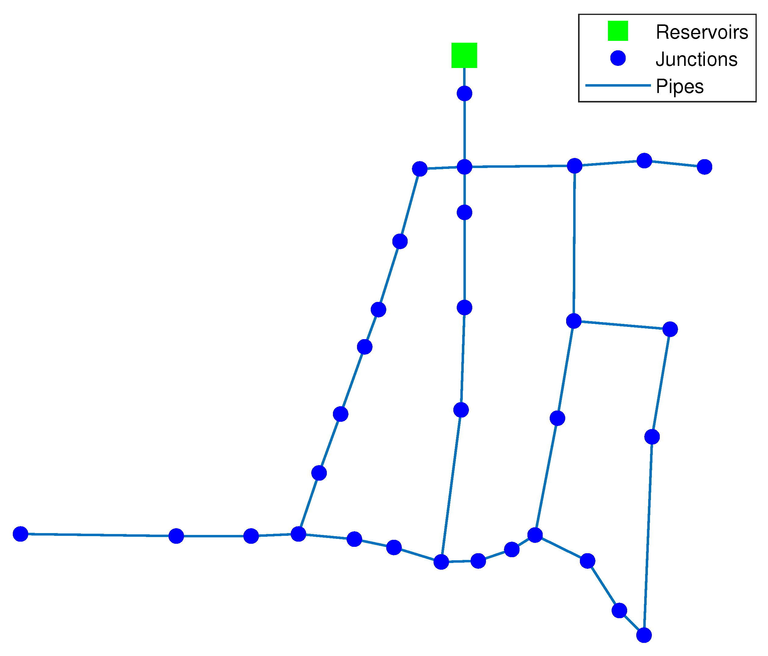
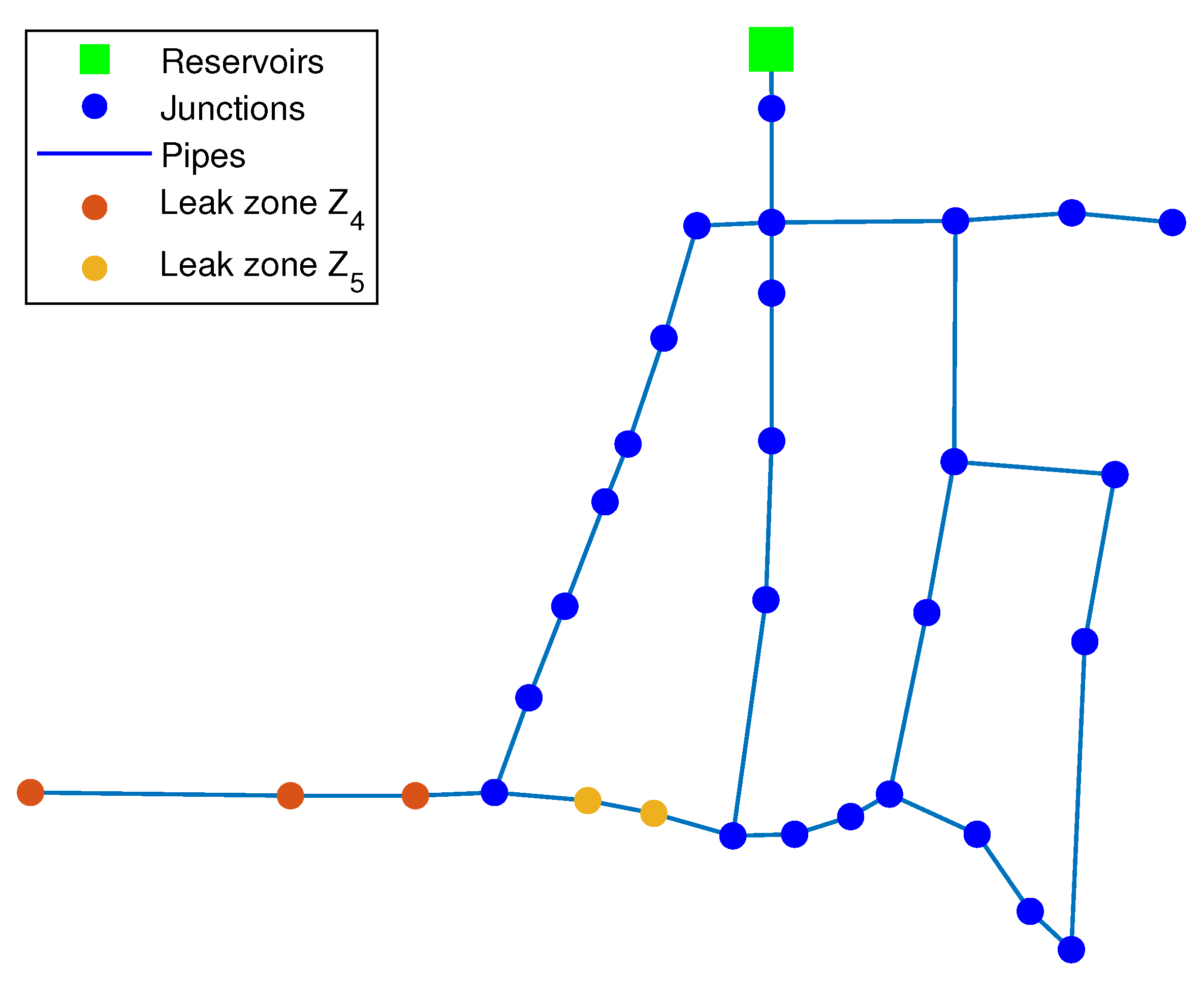
To evaluate the performance of the proposed multi-leak isolation strategy, Hanoi’s WDN is considered since it is a widely used benchmark. This network is built with thirty-one junction nodes, one reservoir and thirty-four pipelines, whose diameters vary between 300 and 1000 mm in diameter; see Figure 3.
This WDN is simulated by using the well-known EPANET-MATLAB Toolkit [40]. It is assumed that the model of the WDN has been calibrated previously on the basis of recorded measurements.
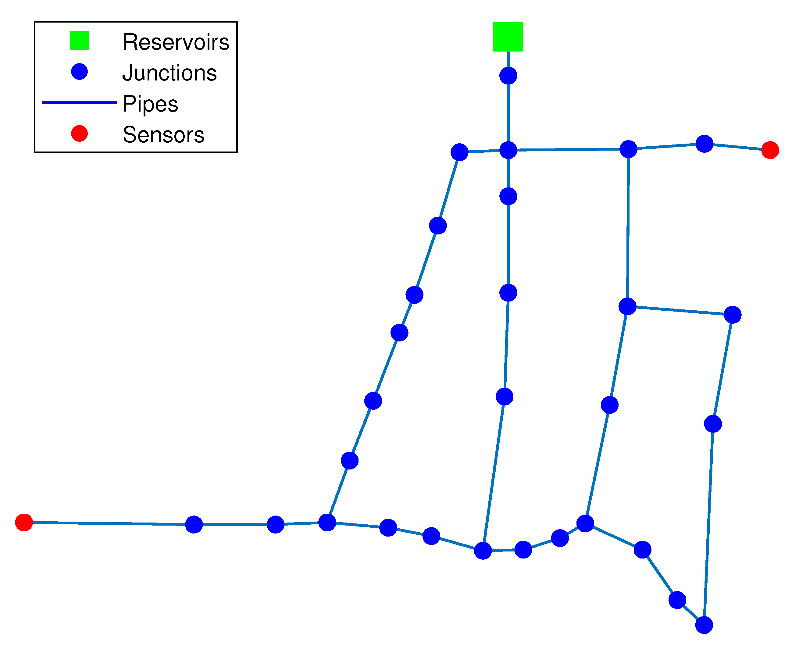
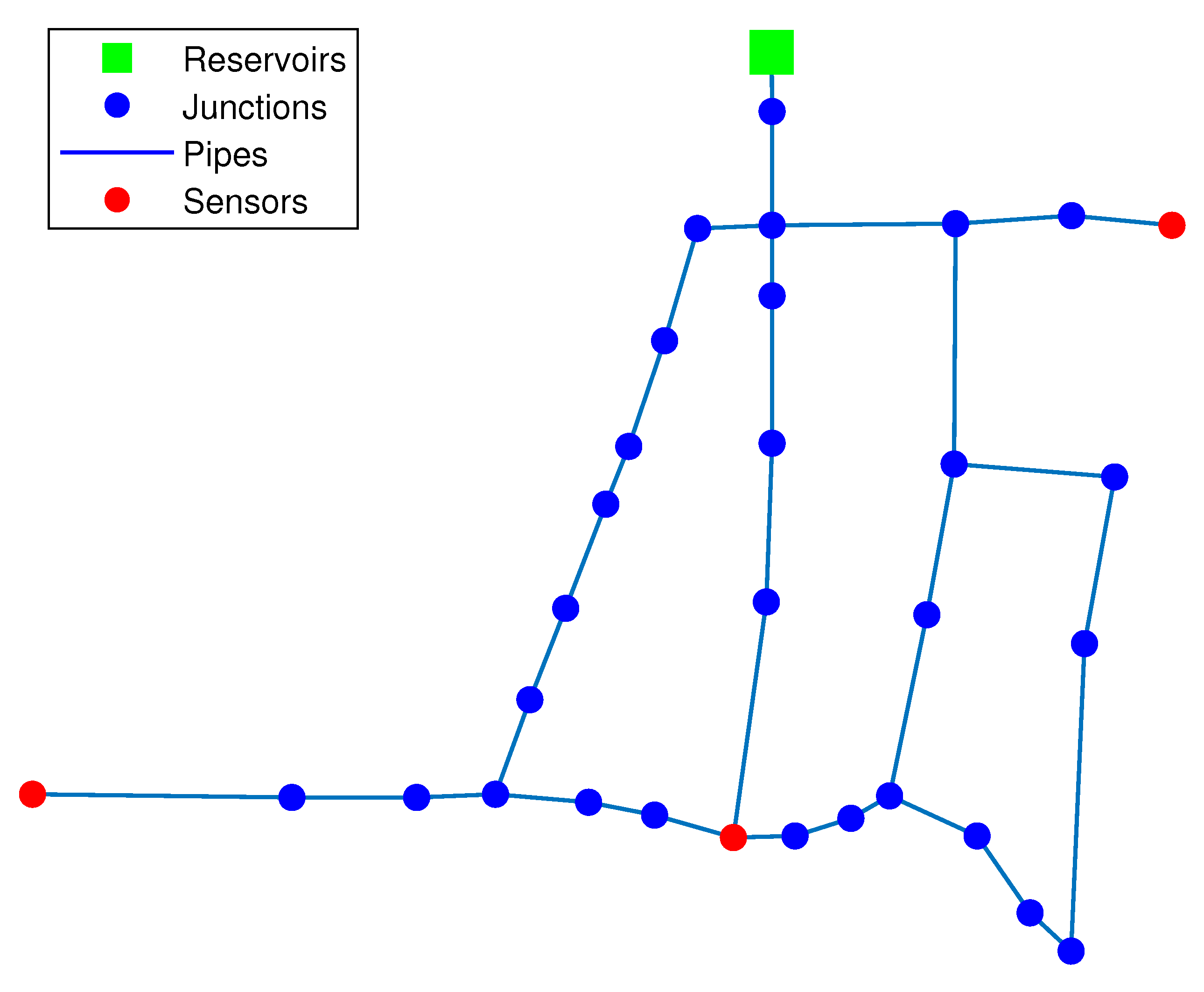
On the other hand, the sensor placement procedure described in Section 2.1 is performed considering the availability of two and three pressure head sensors, respectively. Table 1 presents nodes where the sensors are installed for the two considered sensor configurations.
Figure 4 and Figure 5 present the exact location of the sensors in the network graph.
Similar optimal sensor placement has been obtained for Hanoi’s WDN in [41,42].
Following the procedure presented in Section 2.2.1, for the case of Hanoi’s network n = 31 , a division in p = 11 zones is considered, as shown in Table 2:
Those p zones are depicted in Figure 6.
The number of classes of zones is computed by Equation (13) as follows:
C p = C p 1 + C p 2 = 11 2 + 11 = 66
Notice that this segmentation is not unique; it depends on the designer criteria. On the other hand, it is considered that both leak flow rates can be different q n i q n j and can vary in a range of ( 8 , 80 ) [L/s], which corresponds ( 0.27 , 2.7 ) %, in terms of nominal flow 2890 [L/s]. In this case, each leak flow rate range is divided in r = 10 flow sections; the number of all possible combinations of both ranges is obtained by using the Cartesian product through Equation (18), providing r 2 = 100 . Moreover, the total number of different leak scenarios is computed considering Equation (19) as follows:
L s p = C p r 2 = ( 66 ) ( 100 ) = 6600 .
The resulting residual vector of pressure heads can be computed from a free-leak scenario and those L s p leaky scenarios as described by Equation (20), such that R R 3 × 6600 . It is possible to construct a 24 h residual as in Equation (21). This is the amount of data used for the training of the network. To assess the performance of both classifiers, 200 test cases were created, with leak flow rates ranging from 0.27 % to 2.7 % of the nominal network flow rate. It is important to note that these magnitudes differ from those in the training database. In addition, these magnitudes vary by ± 10 % over the hours of analysis. Furthermore, these tests also took into account uncertainties in the pressure measurements, which are affected by Gaussian noise in a range of ± 5 % relative to the average measured pressure. In the following, three different leak scenarios of two-simultaneous-leak cases are presented.

3.1.1. Leak Scenario A

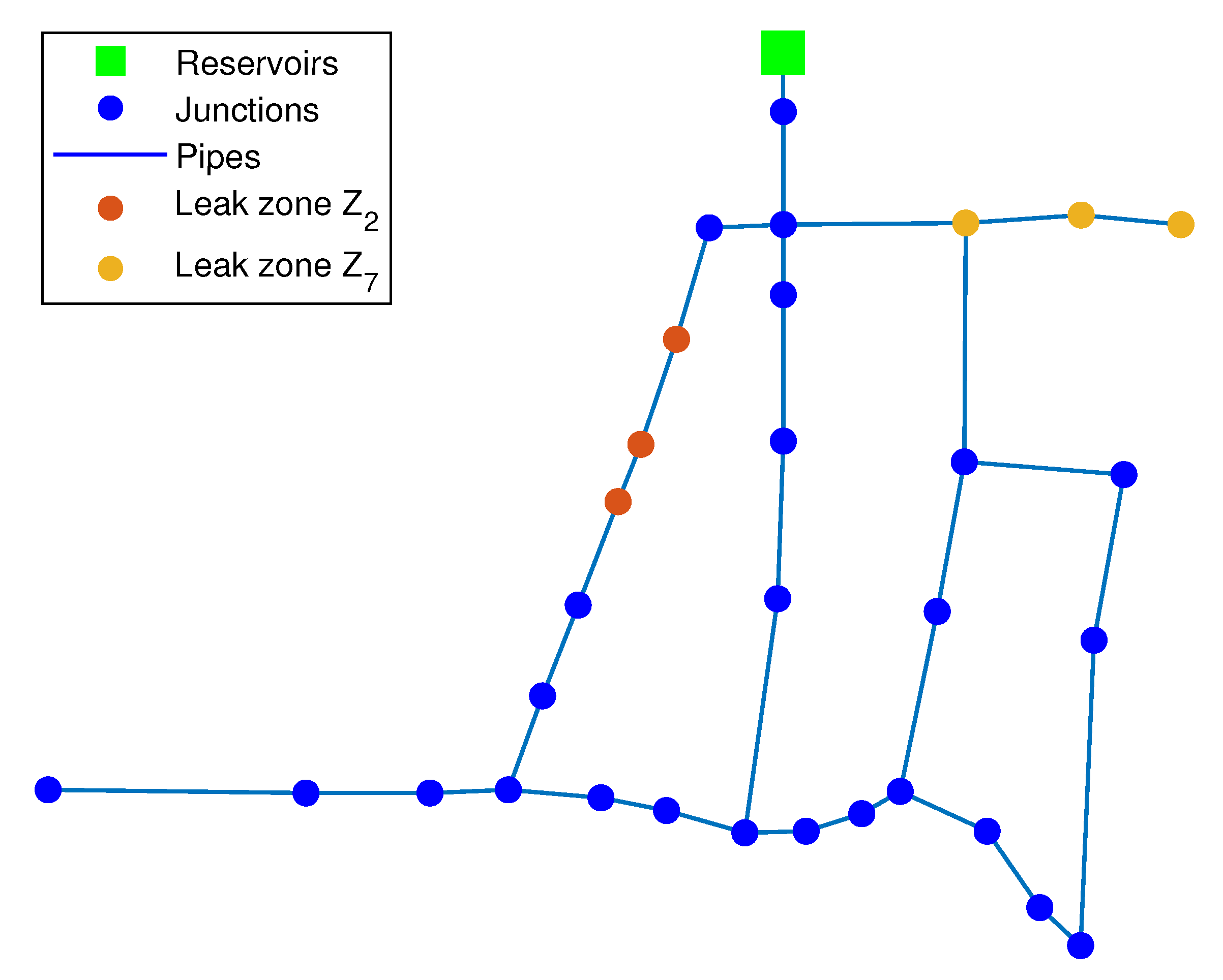
For this case A , two simultaneous leaks occur at nodes 4 and 21, respectively. See Figure 7, whose leakage flow rates are 48 and 11 [L/s], respectively.
This case presented is part of the 200 test cases in which the pressure measurements are corrupted by some noise and also that the leakage rate does not exactly match the values contained in the vector (17). In other words, there are uncertainties, such as pressure head measurements or leak flow rates. In this case, both the k-NN and the DA algorithms estimate exactly the zones in which the pair of leaks are occurring; in other words, z 2 and z 7 have been correctly identified. It should be noted that this identification does not provide the exact leaky nodes. However, the uncertainty is considered, in the worst case, two consecutive nodes far at most. Figure 8 and Figure 9 show the identified zones provided by both algorithms, respectively.
Note that these results are obtained when the analysis of a daily residual is completed, in other words, when the residual vector (21) has been fully analyzed.

3.1.2. Leak Scenario B

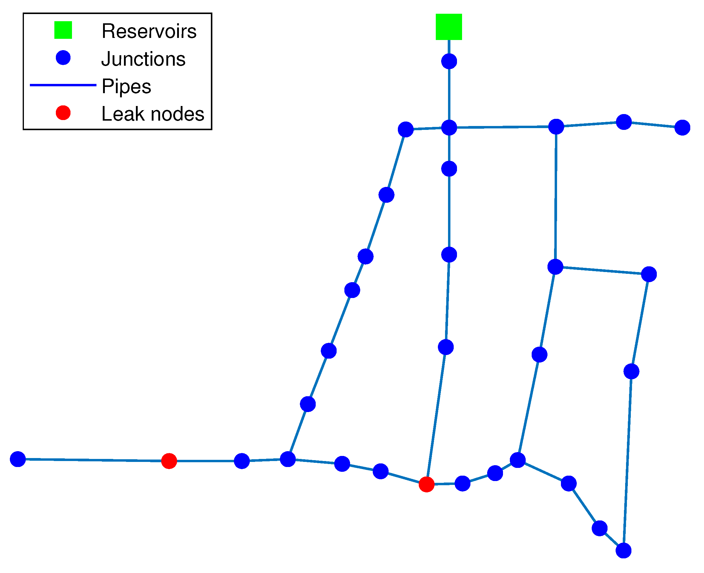
For the second case B , a pair of leaks was simulated at nodes 18 and 28, whose leakage flow rates are 24 and 39 [L/s], respectively, as shown in Figure 10.
As can be seen in Figure 11 and Figure 12, the result obtained by means of the discriminant analysis classifier was better compared to that of the k-NN classifier since the latter failed to identify the area where the node 28 leak is located.

3.1.3. Leak Scenario C

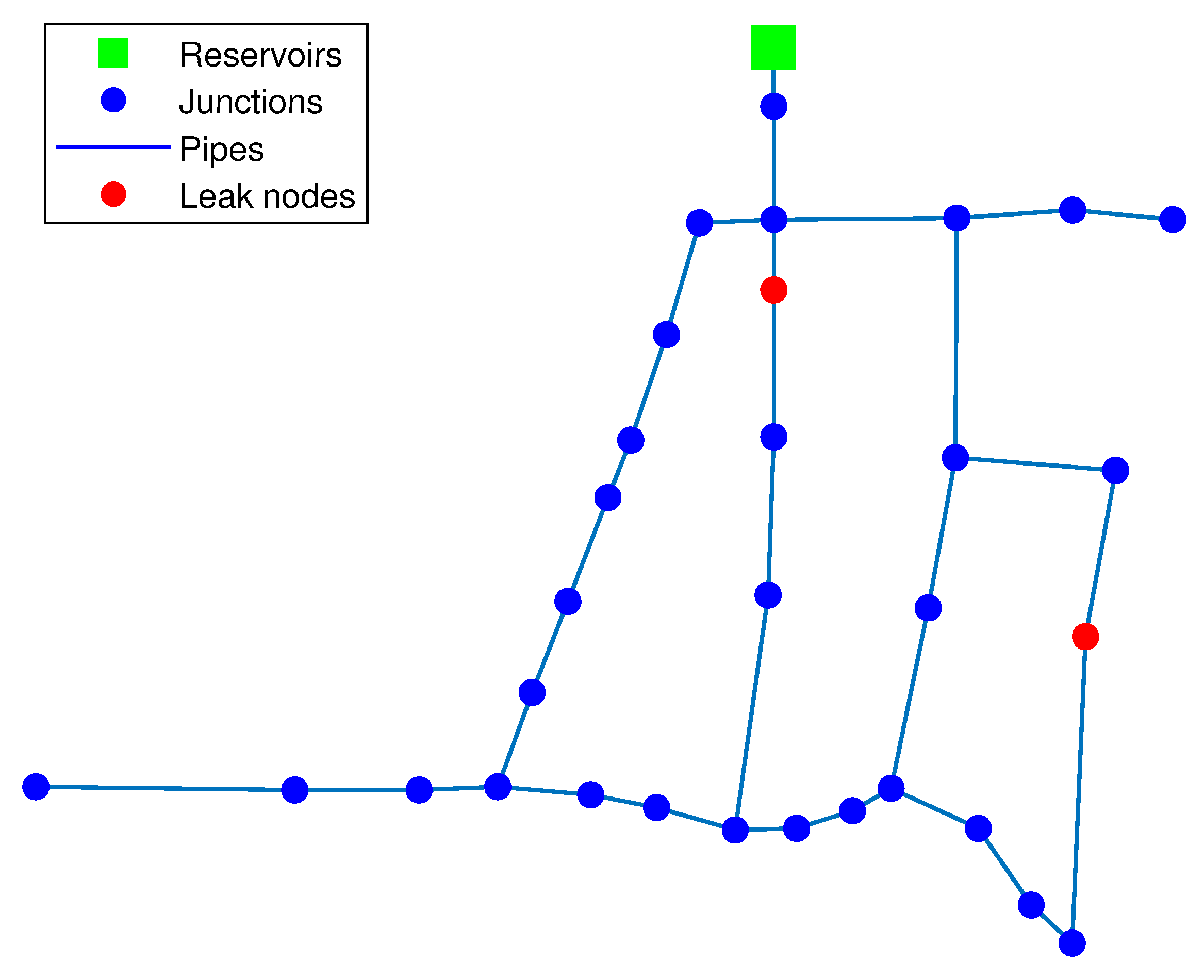
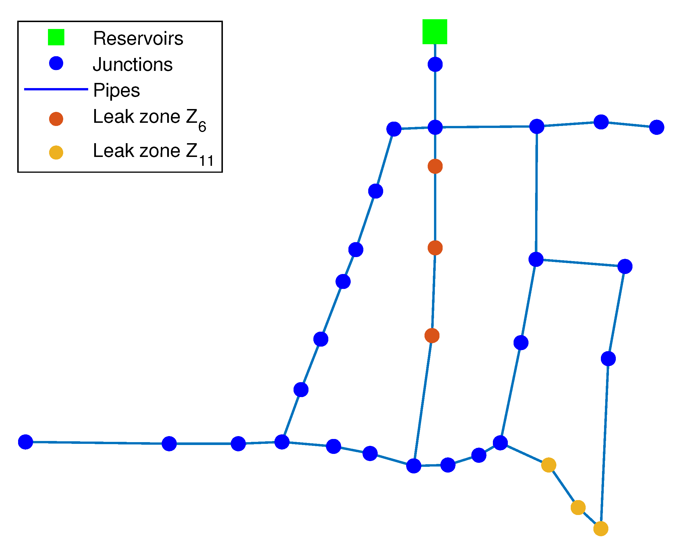
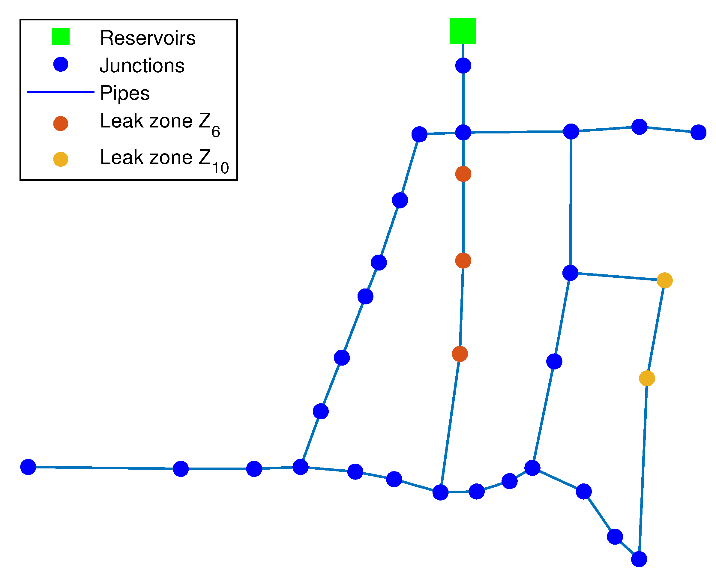
Finally, in the last case, leakage was simulated at node 15 with a 59 [L/s] leak flow and at node 11 with a 46 [L/s] leak flow as can be seen in Figure 13, obtaining candidate zones z 6 and z 11 by means of the k-NN classification (shown in Figure 14), while the candidate zones obtained by the DA classifier are presented in Figure 15.
Once again, it is evident that the k-NN classifier shows inferior performance compared to the discriminant analysis classifier. The k-NN classifier has difficulty in accurately classifying either leakage since its predictions are found to be a maximum of two nodes away from the actual leakage location. The rest of the 200 studies are presented in more detail in the following section, where the relaxation node criterion is also defined to define the usefulness of the results obtained.

3.1.4. Relaxation Node Analysis

As has been shown, sometimes, the leaky zones are not identified with accuracy and an issue arises regarding the obtained result. In other words, to asses how good a result is, a relaxation-node-based criterion is used as in [21]. The one-node relaxation criterion is when the leaky zone is not the correct one. However, the leaky node is just at the left hand side or right hand side of the identified zone; see Figure 16. In the same way, the two-node relaxation criterion is when the leaky node is two nodes far either to the left hand side or the right hand side of the identified leaky zone; see Figure 16.
For both classifiers, in addition to the three leakage cases described in detail, a total of 200 scenarios mentioned above were analyzed using an analysis from a single hour up to 24 h, corresponding to an entire day. From this, it can be noted that the use of recursivity in the classifiers significantly improves their performance compared to tests performed using a single-hour analysis. This analysis allows a more in-depth conclusion about the performance of the proposed multi-leak isolation strategy.
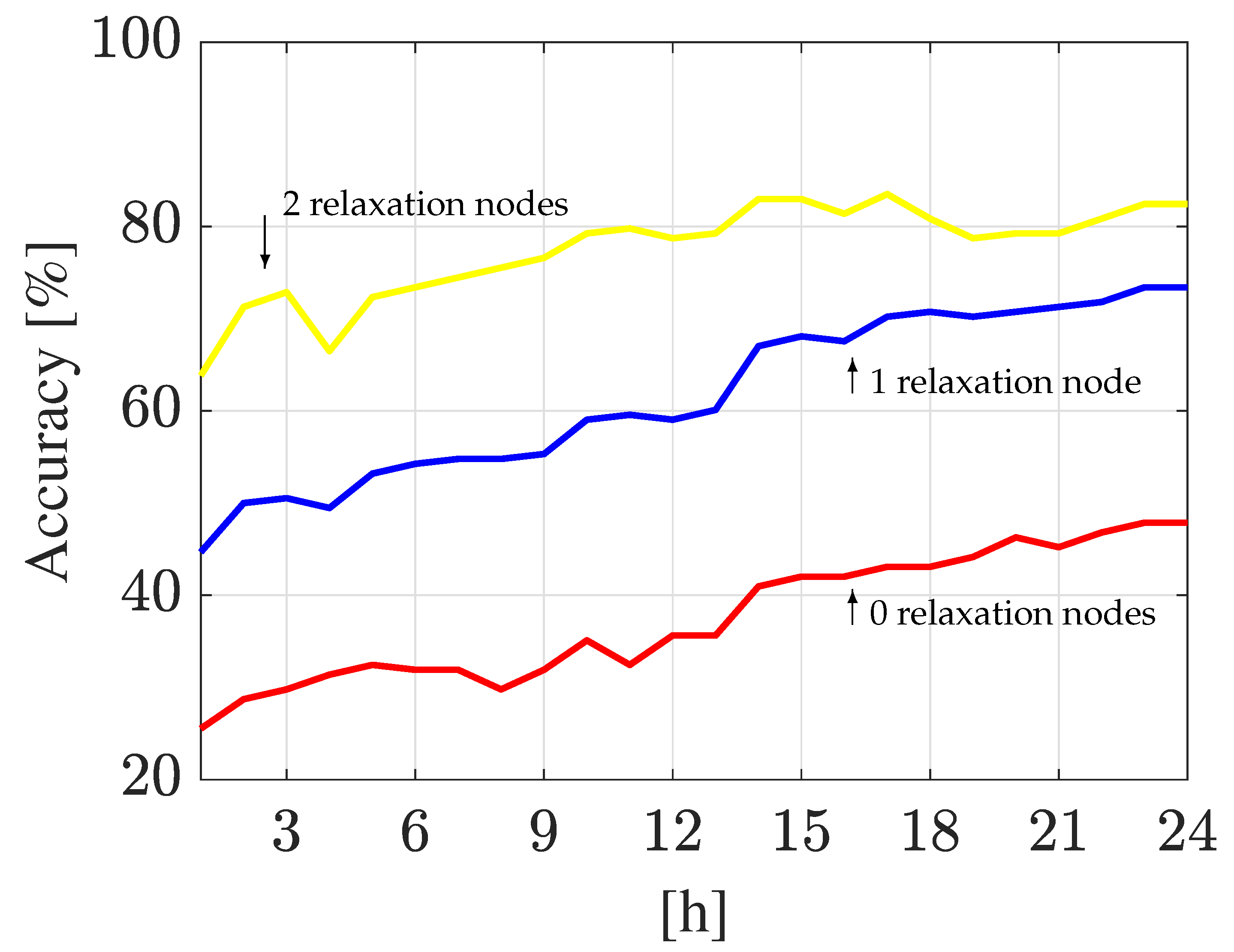
Figure 17 shows the performance of the k-NN-based algorithm. Firstly, it should be noted that the analysis is performed hourly during 24 h . It is highlighted that the accuracy rate improves over time. The exact zone criteria before 12 h show that the accuracy rate is not greater than 40 % , whereas this limit is crossed after that hour and reaches up to 50 % approximately. Moreover, by considering the one node of relaxation criterion, such a rate becomes 60 % and up to 70 % for the same period of time. Finally, if the two nodes of relaxation criterion is considered, the accuracy rate increases from approximately 75 % and up to 80 % , respectively. For the above, these results are considered a good outcome since the leaky node is often close to the leaky identified zone, except in about 20 % of the experiments.
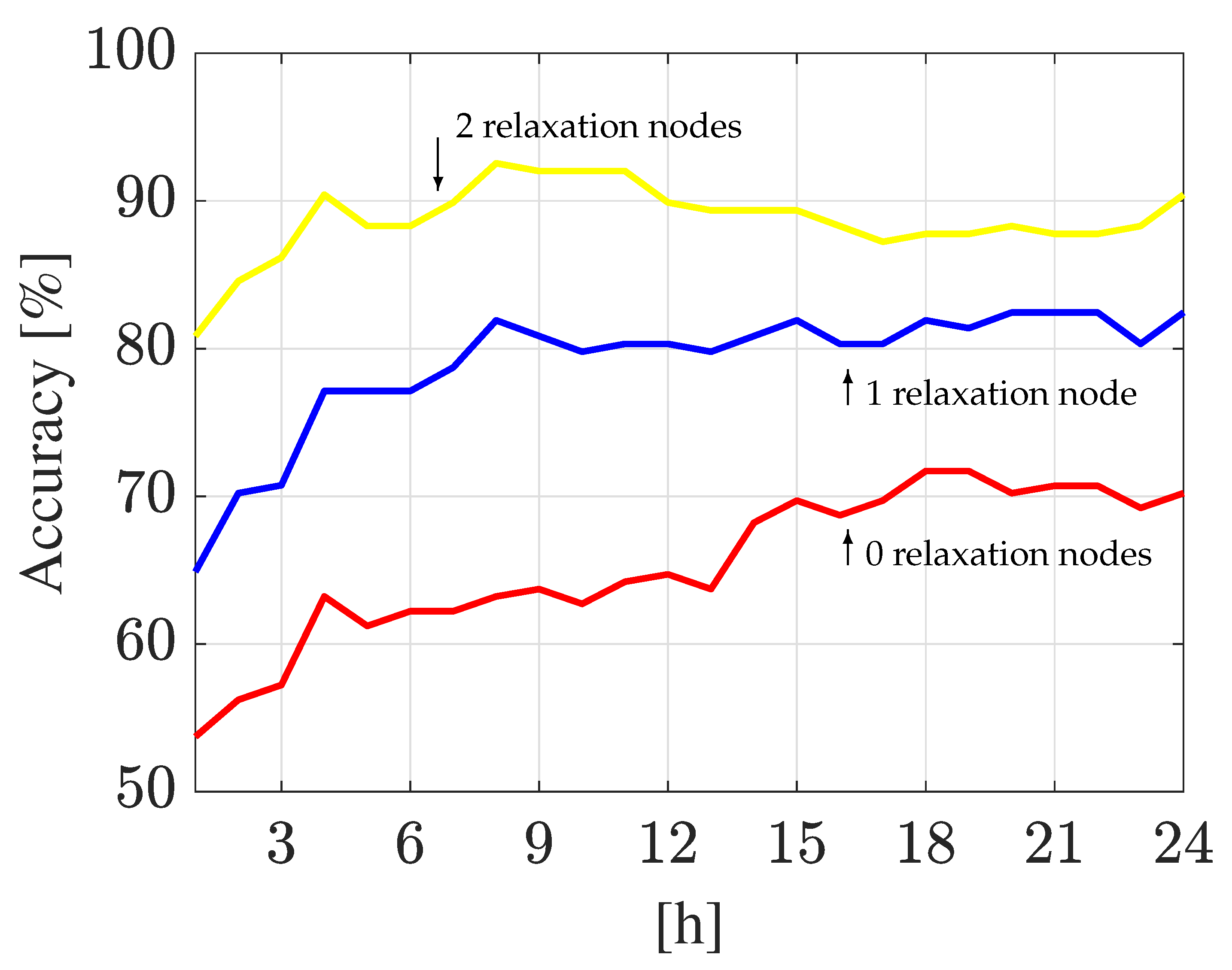
Similarly, the performance of the DA-based algorithm is depicted in Figure 18. It can be seen that, in this case, the accuracy rate is approximately 62 % at 12 h and, after that, it reaches up to 70 % for the exact zone criteria. By considering the one relaxation node criterion, the accuracy rate reaches 80 % at 8 h and remains similar up to the end. Finally, with the two relaxation node criterion, the accuracy rate is 90 % at 6 h , and, as before, it remains similar up to the end.

3.2. Madrid’s DMA Case Study

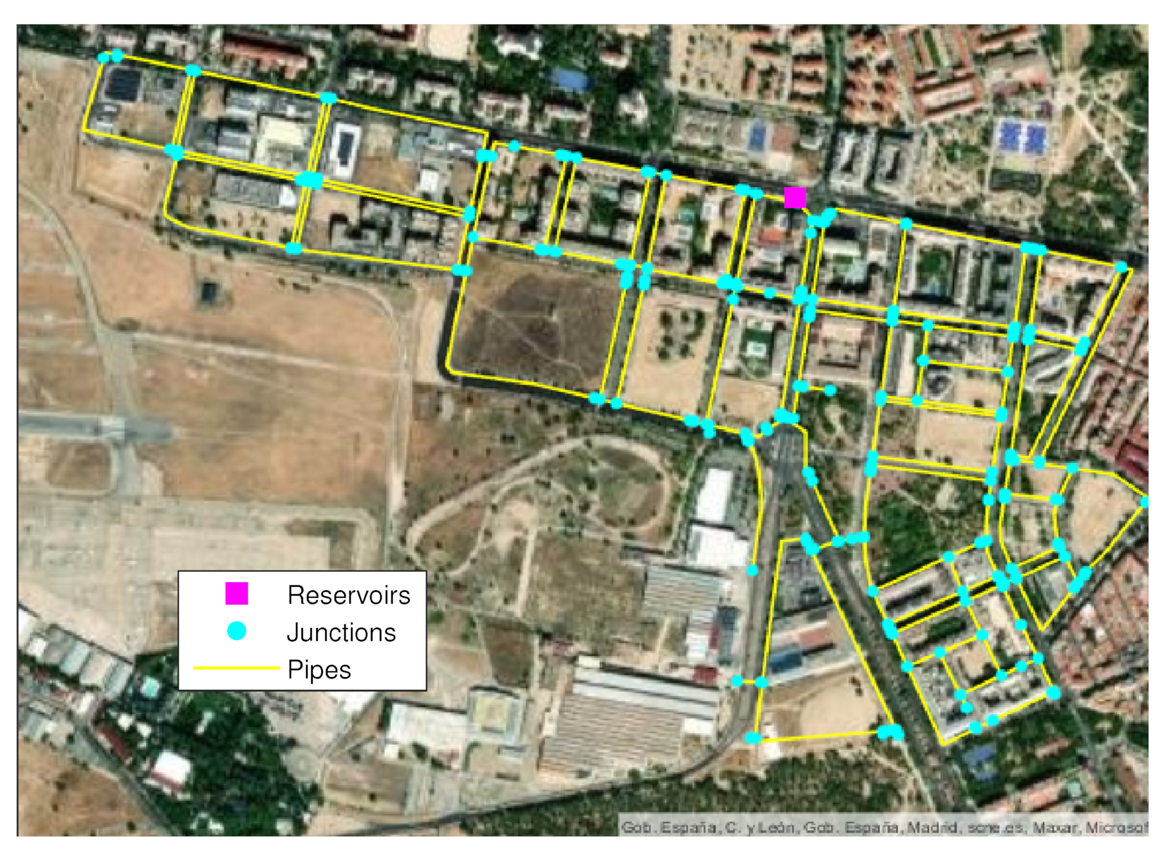
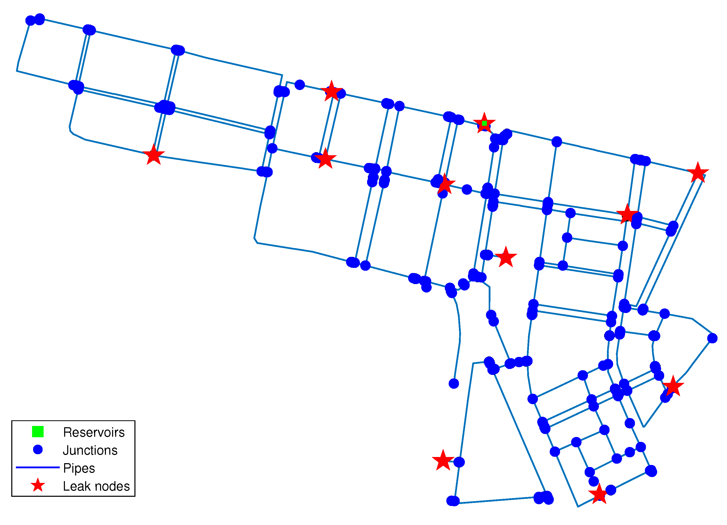
To evaluate the performance of the proposed leak diagnosis methodology, a district metered area (DMA) of a WDN located in Madrid, Spain is considered; see Figure 19. This DMA has one reservoir and three-hundred-twelve nodes, which are interconnected by a network of pipelines of approximately 14 km in length and whose diameters vary between 80 and 350 mm, respectively.
In the same way as before, as a first step, a sensor placement procedure must be performed considering that 11 sensors are available. In this case, due to a large amount of nodes (312), exhaustive testing for an optimal sensor placement is not feasible; a sensor placement as illustrated in Figure 20 is adopted instead, which has been obtained by using techniques based on information theory and genetic algorithms just as in [42].
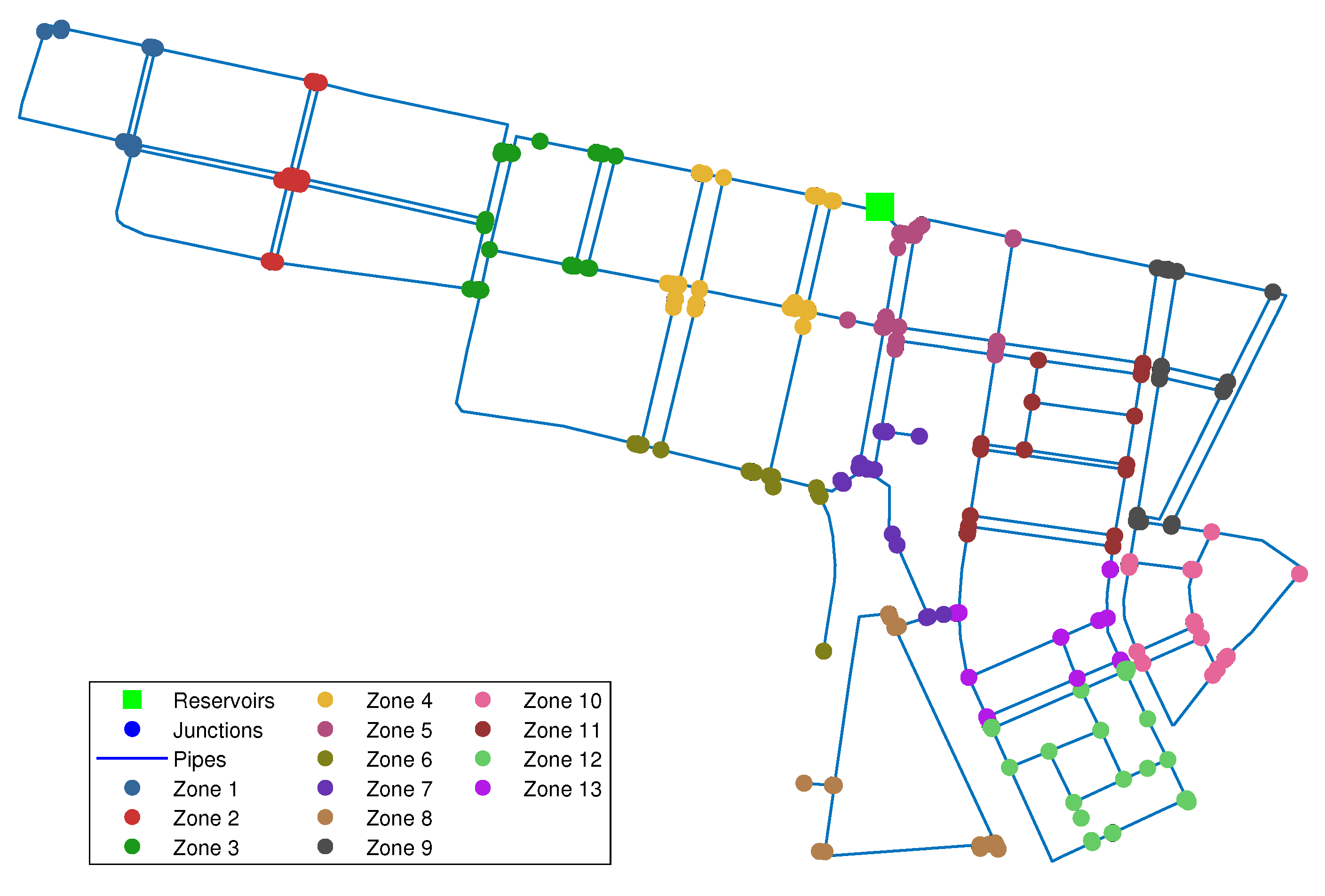
Once the sensor placement procedure has been performed, the following step is to divide the DMA in a reasonable number of zones considering a tradeoff between accuracy and simplicity. On the one hand, a large number of zones leads to a large number of combinations, which, in turn, produces a significant computational cost. On the other hand, due to the computational effort being the main limitation, the reduction in accuracy could be a good election to address large-scale systems. In particular, Madrid’s DMA has been divided into 13 zones as illustrated in Figure 21. It should be noted that the design of zones is not unique.
Following a similar procedure as for the Hanoi WDN, for training purposes, 24-h simulation databases of possible leakage scenarios are generated and stored. To accomplish that, the leak flow rate of each leak can vary in a predefined range; in this case, the lower limit is 0.3 and the upper limit is 1.5 [L/s] for both leaks. Following Equations (14)–(18) with r = 7 , the number of all possible combinations of both ranges is 49 with steps of 0.2 [L/s] and, in terms of nominal flow, this corresponds to 1.6 % and up to 10 % , respectively. On the other hand, to quantify the performance of both classifiers, in this case study, 200 random leakage cases were generated for testing. Those cases have leakage magnitudes within a range of 0.3 to 1.5 [L/s], including an uncertainty of ± 10 % . In addition, the pressure head measurements are corrupted by a Gaussian noise of ± 5 % to evaluate the robustness of the classifiers under this situation.
Hereinafter, the obtained results are presented considering both one and two relaxation node criteria.

Relaxation Node Analysis

Similar as before, the relaxation node criteria shown in Figure 16 are used. On the one hand, the k-NN classifier had an accuracy rate less than 40 % during the 24 h period of analysis when neither relaxation node criteria are considered. For the one relaxation criterion, this classifier increased its accuracy rate from 30 % and it reaches up to 45 % at the end of the analysis. Finally, for the two relaxation node criterion, the accuracy rate begins with 38 % and reaches up to 50 % at 15 h and remains at this level up to the end of the analysis; see Figure 22.
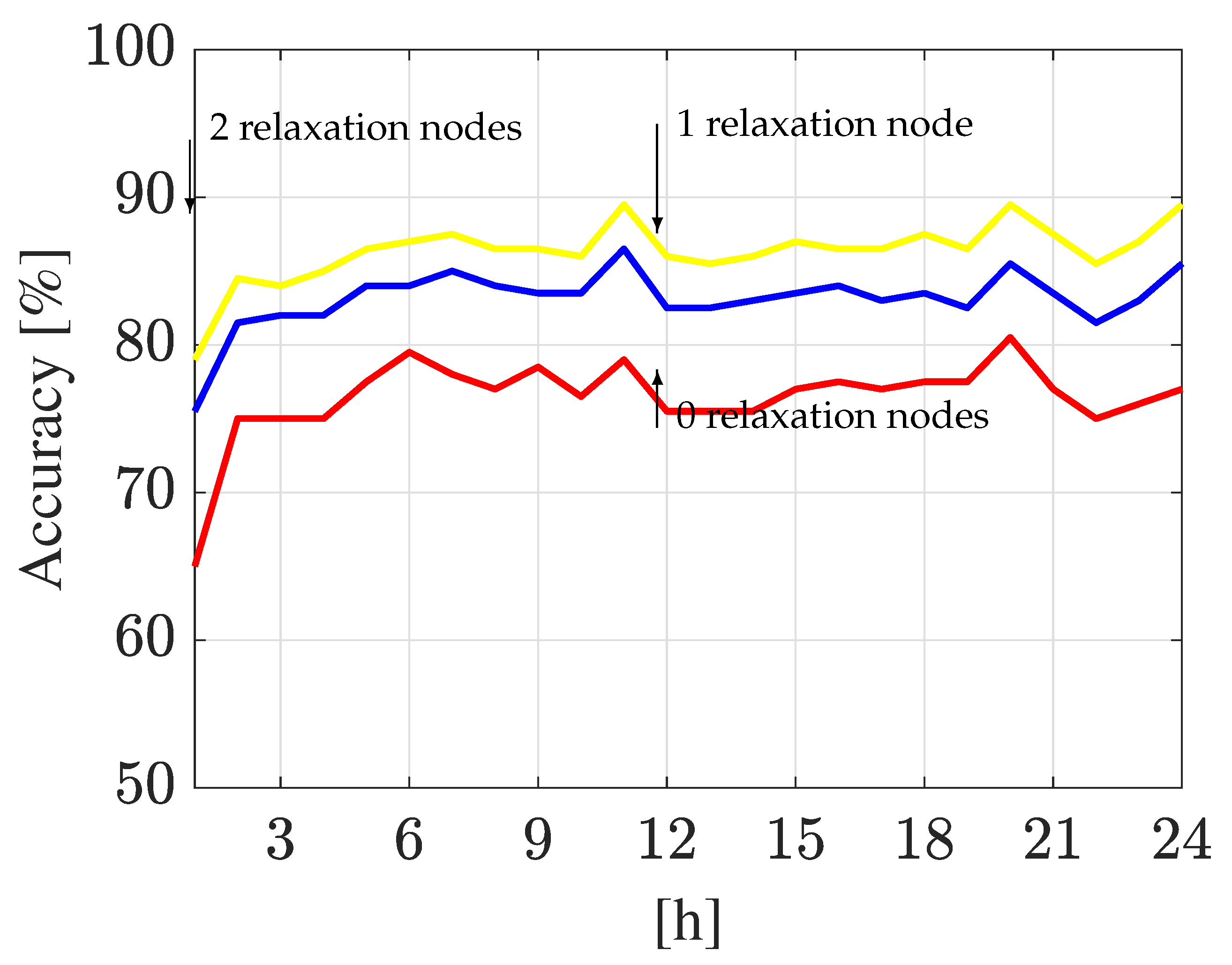
On the other hand, from Figure 23, it can be observed that the DA-based classifier had an accuracy rate of 65 % at the beginning and it reaches up to 75 % at the end of the analysis when the one relaxation node criterion is considered. Moreover, when the two relaxation node criterion is used, the accuracy rate reaches up to 80 % , respectively. Furthermore, when no relaxation nodes are used, the accuracy rate reaches a value of 79 % at 6 h, which is relatively maintained until 20 h when it declines in the last four hours of the analysis, decreasing up to 77 % at 24 h.

3.3. Discussion

The proposed methodology is focused on identifying the leaky zones rather than the leaky nodes. This criterion makes a good tradeoff between accuracy and simplicity due to the complexity that this two-simultaneous-leak problem represents by itself. In spite of this, the solution of this complex leak localization problem can be considered as a good outcome since the leak search area is reduced to a limited set of neighbor nodes.
Comparing both case studies, it can be observed that, as the complexity of the network increases (number of nodes), the accuracy rate of the k-NN algorithm decreases significantly. Conversely, the DA-based algorithm maintains a similar accuracy rate no matter the network complexity. In Table 3, a comparison of the performance of both classifiers is summarized. Here, N h stands for the number of hours in which the analysis has been performed.
It should be noted that the accuracy rate varies significantly when the relaxation node criteria are used, but it depends on the number of nodes that belong to the same zone (accuracy level). However, this is a direct consequence of using a segmentation of the WDN, especially for large-scale systems. This can be observed in the Table 3, where, for both classifiers in the Hanoi network, there is a higher increase in accuracy using relaxation node criteria compared to the accuracy obtained in the Madrid DMA.
The decrement in the classification of the k-NN algorithm results can be attributed to factors like not having a wide separation between the data that make up each class so that, for several cases, deficient classification results are obtained. A possible alternative to enhance this outcome is to adapt the number of k-nearest neighbors based on each case study and the amount of data for training; however, this does not guarantee a significant improvement in the results of the classifier.
Finally, although the linear discriminant analysis classifier seems to yield more consistent accuracy rates in Madrid’s DMA case study, this does not necessarily imply a better performance compared to the classification performed in the Hanoi network model since it should be considered that, in the Hanoi network, there are zones with fewer nodes.

4. Conclusions

The proposed methodology demonstrated to be an efficient tool to address the two-simultaneous-leak problem in water distribution networks. The segmentation of the network in zones reduced significantly the computational cost by maintaining a good tradeoff between simplicity and accuracy. Although exact leaky node identification is hard to achieve, the decision to identify a zone rather than a node keeps the uncertainty of the actual location of the leak under control. In other words, the leak node is often in the identified zone, which allows a significant reduction in the final leak search. When Madrid’s DMA case study is considered, the performance of the DA-based classifier is still robust regardless of the network’s size. This is possible because such a network is divided into a reasonable number of zones.
It should be noted that, in each case study, the proposed segmentation in zones causes a reduction in the size of the residual vector that would be generated by all possible scenarios of two simultaneous leaks in the network. For the Hanoi case study, there is a reduction from 46,500 leak scenarios to 6600, which, in turn, represents a reduction in the computational cost.
It has also been highlighted that, although in some cases both classifiers fail to identify the exact zone where the leak is occurring, the leaky node is close, and the relaxation node criteria allow to somehow define the uncertainty of the obtained result. In particular, the k-NN classifier showed an overall lower performance compared to the DA-based classifier. Hence, as a future work, it would be of interest to conduct an analysis using other classifiers to assess their performance.
In addition, it should be noted that, in this work, the initial prior probability of both classifiers was set equal to each class, which means that the occurrence of leaks is equally probable for any area of the network. However, in practice, there may be certain zones where the occurrence of leaks is higher due to factors such as pipe aging, greater susceptibility to seismic damage, historical records of failures in the network, etc. Therefore, as a future work, an analysis taking into account some of those factors to establish the initial prior probabilities is of particular interest.
The sensor placement methodology here adopted was designed for a single-leak scenario. Therefore, the development of a sensor placement methodology specifically designed to address multiple simultaneous leaks scenarios could enhance the obtained results.
Finally, a more-in-depth analysis on the zone segmentation of a WDN by using more complex criteria is required to establish an optimal tradeoff between simplicity and accuracy. On the other hand, a study about the variation in the sampling rate is also needed since, in practice, the devices are not able to provide measurements with a high sampling rate. Both issues will be part of future developments.

Author Contributions

Conceptualization, C.A.R.-A., O.B.-M. and J.A.D.-A.; Data curation, C.A.R.-A.; Formal analysis, J.A.D.-A. and I.S.-R.; Methodology, C.A.R.-A. and J.A.D.-A.; Project administration, J.A.D.-A.; Software, C.A.R.-A.; Supervision, O.B.-M. and J.A.D.-A.; Validation, C.A.R.-A.; Visualization, A.N.-D., I.S.-R. and J.A.D.-A.; Writing—original draft, C.A.R.-A., O.B.-M., J.A.D.-A., I.S.-R., V.P. and A.N.-D.; Writing—review and editing, C.A.R.-A., O.B.-M., J.A.D.-A., I.S.-R., V.P. and A.N.-D. All authors have read and agreed to the published version of the manuscript.

Funding

The APC was funded by Tecnológico de Monterrey.

Data Availability Statement

Not applicable.

Acknowledgments

The first author would like to acknowledge CONACYT for its support via the master fellowship 244269, but also CIIDETEC-UVM, IRI-UPC and TURIX-Dynamics Diagnosis and Control Group of Tecnológico Nacional de México for their fruitful collaboration in this research.

Conflicts of Interest

The authors declare no conflicts of interest.

Abbreviations

    The following abbreviations are used in this manuscript:
AIArtificial Intelligence
WDNWater Distribution Network
OECDOrganization for Economic Cooperation and Development
FIRFinite Impulse Response
RBFRadial Base Function
DADiscriminant Analysis
k-NNk Nearest Neighbors
hHour
L/sLiters per second
f R Leak flow rate used for estimation of residuals
f S Leak flow rate used for estimation of sensitivities
R Set of real numbers
diagDiagonal matrix
maxMaximum Value
arg maxMaximum argument

Appendix A. Sensor-Placement-Methodology-Based Algorithm

Algorithm A1: Sensor-placement-methodology-based algorithm.
Require :
The number of sensors to place N s , the number of nodes n, the leak flow for residuals f R , the leak flow for the sensitivity matrix f S , the matrix L R n × d containing all the possible locations of the sensors, where d is computed as n N s .
Ensure :
L o p t as the optimal sensor placement
1:
Load the model file of the water distribution network model.
2:
Get  p ^ the pressure of every node in a free-leak scenario.
3:
Calculate Matrices S and R using the leak flows f S and f R for sensibility and residuals Equations (5) and (6).
4:
e m i n n
5:
for  i = 1 : d   do
6:
     L i d i a g ( L ( i , : ) )
7:
     S L L i · S
8:
     R L L i · R
9:
     e 0
10:
    for  a = 1 : n  do
11:
         ψ a a R L a T · S L a R L a S L a Equation (8).
12:
        for  b = 1 : n  do
13:
              ψ a b = R L a T · S L b R L a S L b Equation (8).
14:
             if  ψ a b > ψ a a  then
15:
                  e e + 1
16:
                 break for
17:
           end if
18:
        end for
19:
        if  e > e m i n  then
20:
           break for
21:
        end if
22:
    end for
23:
    if  e e m i n  then
24:
         e m i n e
25:
         L o p t L i
26:
    end if
27:
end for print  L o p t

Appendix B. Dataset-Generation-Methodology-Based Algorithm

Algorithm A2: Dataset-generation-methodology-based algorithm
Require :
A network model, the number of zones into which the network is divided p, and the nodes that conform each zone, a set of N s nodes where the pressure sensors are located, the leakage flow rate for the two leaky nodes q n i and q n j having a previously defined range r.
1:
Load the model file of the water distribution network model.
2:
Get  p ^ the pressure of sensor in a free-leak scenario during 24 h.
3:
C p C p 2 + p Equation (13)
4:
Create Class labels with the zone combinations for each of the C p classes.
5:
Q q n i × q n j   Equation (18)
6:
L s p C p r 2   Equation (19)
7:
Create A zeros matrix R R N s × L s p
8:
for  a = 1 : C p do
9:
    for  b = 1 : r 2  do
10:
         i ( a 1 ) r 2 + b
11:
         L a set of two nodes belonging to each of the zones of the class a.
12:
        Compute Residual vector δ using nodes L and Q ( b ) flow rates, δ R N s × 1 .
13:
         R ( : , i ) δ
14:
    end for
15:
end for
16:
Assign the columns of R to their corresponding classes.
17:
Output The C p class labels, Training dataset R .

Appendix C. Leak-Localization-Strategy-Based Algorithm

Algorithm A3: Leak-localization-strategy-based algorithm
Require :
A set of residuals per hour r starting from the time the presence of leaks is detected, the training dataset R , whose columns are ordered from the hour the leaks are detected for a 24 h analysis, The class labels Y of the C p classes and the prior probability P p r i o r of each class to be the leaky zones.
1:
P K N N p r P p r i o r .
2:
P D A p r P p r i o r .
3:
for   h = 1 : 24 do
4:
    Set  x r As the r residual vector of the h-th hour of analysis.
5:
    Set  X As the column of R at the analysis hour h.
6:
    Train k-NN model with X and Y
7:
    Set k-NN model prior probability as P K N N p r
8:
    Train DA model with X and Y
9:
    Set DA Model prior probability as P D A p r
10:
     Z K N N k-NN model Predict of x r
11:
     Z D A DA model Predict of x r
12:
     P K N N p t k-NN model post probabilities
13:
     P D A p t DA model post probabilities
14:
    if  M a x ( P K N N p t ) = = 1  then
15:
        Set  M a x ( P K N N p t ) 0.99
16:
        Set the other elements of P K N N p t 0.01 ( C p 1 )
17:
    end if
18:
    if  M a x ( P D A p t ) = = 1  then
19:
        Set  M a x ( P D A p t ) 0.99
20:
        Set the other elements of P D A p t 0.01 ( C p 1 )
21:
    end if
22:
     P K N N p r P K N N p t .
23:
     P D A p r P D A p t .
24:
end for
25:
Output The candidate Z K N N of the k-NN model, the candidate zone Z D A of the DA model.

References

  1. OECD. Water Governance in Cities; OECD: Paris, France, 2016; p. 140. [Google Scholar] [CrossRef]
  2. Puust, R.; Kapelan, Z.; Savic, D.A.; Koppel, T. A review of methods for leakage management in pipe networks. Urban Water J. 2010, 7, 25–45. [Google Scholar] [CrossRef]
  3. Kim, H.; Shin, E.; Chung, W. Energy demand and supply, energy policies, and energy security in the Republic of Korea. Energy Policy 2011, 39, 6882–6897. [Google Scholar] [CrossRef]
  4. Qi, S.; Gao, J.; Wu, W.; Qiao, Y.; Tu, M.; Wang, J. Research on an Optimized Leakage Locating Model in Water Distribution System. Procedia Eng. 2014, 89, 1569–1576. [Google Scholar] [CrossRef]
  5. Delgado-Aguiñaga, J.A.; Begovich, O. Water Leak Diagnosis in Pressurized Pipelines: A Real Case Study; Springer International Publishing: Cham, Switzerland, 2017; pp. 235–262. [Google Scholar] [CrossRef]
  6. Santos-Ruíz, I.; Bermúdez, J.; López-Estrada, F.; Puig, V.; Torres, L.; Delgado-Aguiñaga, J. Online leak diagnosis in pipelines using an EKF-based and steady-state mixed approach. Control. Eng. Pract. 2018, 81, 55–64. [Google Scholar] [CrossRef]
  7. Navarro-Díaz, A.; Delgado-Aguiñaga, J.A.; Begovich, O.; Besançon, G. Two Simultaneous Leak Diagnosis in Pipelines Based on Input-Output Numerical Differentiation. Sensors 2021, 21, 8035. [Google Scholar] [CrossRef] [PubMed]
  8. Torres, L.; Verde, C.; Molina, L. Leak diagnosis for pipelines with multiple branches based on model similarity. J. Process. Control. 2021, 99, 41–53. [Google Scholar] [CrossRef]
  9. Delgado-Aguiñaga, J.; Santos-Ruiz, I.; Besançon, G.; López-Estrada, F.; Puig, V. EKF-based observers for multi-leak diagnosis in branched pipeline systems. Mech. Syst. Signal Process. 2022, 178, 109198. [Google Scholar] [CrossRef]
  10. Fuentes-Mariles, O.; Palma-Nava, A.; Rodriguez-Vazquez, K. Estimation and location of leaks in a drinking water pipeline network using genetic algorithms. Ing. Investig. Tecnol. 2011, 12, 235–242. [Google Scholar] [CrossRef]
  11. Puig, V.; Ocampo-Martínez, C.; Pérez, R.; Cembrano, G.; Quevedo, J.; Escobet, T. Real-Time Monitoring and Operational Control of Drinking-Water Systems; Springer: Cham, Switzerland, 2017; p. 428. [Google Scholar] [CrossRef]
  12. Choi, J.; Jeong, G.; Kang, D. Multiple Leak Detection in Water Distribution Networks Following Seismic Damage. Sustainability 2021, 13, 8306. [Google Scholar] [CrossRef]
  13. Alves, D.; Blesa, J.; Duviella, E.; Rajaoarisoa, L. Multi-leak detection and isolation in water distribution networks. In Proceedings of the 2nd International Joint Conference on Water Distribution Systems Analysis & Computing and Control in the Water Industry, Valencia, Spain, 18–22 July 2022. [Google Scholar]
  14. Vanijjirattikhan, R.; Khomsay, S.; Kitbutrawat, N.; Khomsay, K.; Supakchukul, U.; Udomsuk, S.; Suwatthikul, J.; Oumtrakul, N.; Anusart, K. AI-based acoustic leak detection in water distribution systems. Results Eng. 2022, 15, 100557. [Google Scholar] [CrossRef]
  15. Yang, J.; Wen, Y.; Li, P. Leak acoustic detection in water distribution pipelines. In Proceedings of the 2008 7th World Congress on Intelligent Control and Automation, Chongqing, China, 25–27 June 2008; pp. 3057–3061. [Google Scholar] [CrossRef]
  16. Iwanaga, M.; Brennan, M.; Almeida, F.; Scussel, O.; Cezar, S. A laboratory-based leak noise simulator for buried water pipes. Appl. Acoust. 2022, 185, 108346. [Google Scholar] [CrossRef]
  17. Fan, H.; Tariq, S.; Zayed, T. Acoustic leak detection approaches for water pipelines. Autom. Constr. 2022, 138, 104226. [Google Scholar] [CrossRef]
  18. Pérez, R.; Puig, V.; Pascual, J.; Quevedo, J.; Landeros, E.; Peralta, A. Methodology for leakage isolation using pressure sensitivity analysis in water distribution networks. Control. Eng. Pract. 2011, 19, 1157–1167. [Google Scholar] [CrossRef]
  19. Pérez, R.; Quevedo, J.; Puig, V.; Nejjari, F.; Cugueró, M.; Sanz, G.; Mirats, J. Leakage isolation in water distribution networks: A comparative study of two methodologies on a real case study. In Proceedings of the 2011 19th Mediterranean Conference on Control & Automation (MED), Corfu Island, Greece, 21–23 June 2011; pp. 138–143. [Google Scholar] [CrossRef]
  20. Ponce, M.V.C.; Castañón, L.E.G.; Cayuela, V.P. Model-based leak detection and location in water distribution networks considering an extended-horizon analysis of pressure sensitivities. Hydroinformatics 2014, 16, 649–670. [Google Scholar] [CrossRef]
  21. Soldevila, V.; Tornil-Sin, S.; Blesa, J.; Fernandez-Canti., R.; Puig, V. Modeling and Monitoring of Pipelines and Networks Advanced Tools for Automatic Monitoring and Supervision of Pipelines; Springer International Publishing: Berlin/Heidelberg, Germany, 2017. [Google Scholar]
  22. Carreño-Alvarado, E.; Reynoso-Meza, G.; Montalvo, I.; Izquierdo, J. A comparison of machine learning classifiers for leak detection and isolation in urban networks. In Proceedings of the Congress on Numerical Methods in Engineering CMN 2017, Valencia, Spain, 3–5 July 2017. [Google Scholar]
  23. Romero-Tapia, G.; Fuente, M.; Puig, V. Leak Localization in Water Distribution Networks using Fisher Discriminant Analysis. In Proceedings of the 10th IFAC Symposium on Fault Detection, Supervision and Safety for Technical Processes SAFEPROCESS, Warsaw, Poland, 29–31 August 2018. [Google Scholar] [CrossRef]
  24. Sun, C.; Parellada, B.; Puig, V.; Cembrano, G. Leak Localization in Water Distribution Networks Using Pressure and Data-Driven Classifier Approach. Water 2020, 12, 54. [Google Scholar] [CrossRef]
  25. Ferrandez-Gamot, L.; Busson, P.; Blesa, J.; Tornil-Sin, S.; Puig, V.; Duviella, E.; Soldevila, A. Leak Localization in Water Distribution Networks using Pressure Residuals and Classifiers. IFAC-PapersOnLine 2015, 48, 220–225. [Google Scholar] [CrossRef]
  26. Santos-Ruiz, I.; Blesa, J.; Puig, V.; López-Estrada, F. Leak localization in water distribution networks using classifiers with cosenoidal features. IFAC-PapersOnLine 2020, 53, 16697–16702. [Google Scholar] [CrossRef]
  27. Cordoba, G.C.; Tuhovčák, L.; Tauš, M. Using Artificial Neural Network Models to Assess Water Quality in Water Distribution Networks. Procedia Eng. 2014, 70, 399–408. [Google Scholar] [CrossRef]
  28. Przystałka, P. Performance optimization of a leak detection scheme for water distribution networks. IFAC-PapersOnLine 2018, 51, 914–921. [Google Scholar] [CrossRef]
  29. Basnet, L.; Brill, D.; Ranjithan, R.; Mahinthakumar, K. Supervised Machine Learning Approaches for Leak Localization in Water Distribution Systems: Impact of Complexities of Leak Characteristics. J. Water Resour. Plan. Manag. 2023, 149, 04023032. [Google Scholar] [CrossRef]
  30. Sourabh, N.; Timbadiya, P.; Patel, P.L. Leak detection in water distribution network using machine learning techniques. ISH J. Hydraul. Eng. 2023, 7, 1–19. [Google Scholar] [CrossRef]
  31. Javadiha, M.; Blesa, J.; Soldevila, A.; Puig, V. Leak Localization in Water Distribution Networks Using Deep Learning. In Proceedings of the 2019 6th International Conference on Control, Decision and Information Technologies (CoDIT), Paris, France, 23–26 April 2019; pp. 1426–1431. [Google Scholar] [CrossRef]
  32. Örn Garðarsson, G.; Boem, F.; Toni, L. Graph-Based Learning for Leak Detection and Localisation in Water Distribution Networks. IFAC-PapersOnLine 2022, 55, 661–666. [Google Scholar] [CrossRef]
  33. Hu, Z.; Shen, D.; Chen, W. Deep learning-based burst location with domain adaptation across different sensors in water distribution networks. Comput. Chem. Eng. 2023, 176, 108313. [Google Scholar] [CrossRef]
  34. Arbesser-Rastburg, G.; Fuchs-Hanusch, D. Serious Sensor Placement—Optimal Sensor Placement as a Serious Game. Water 2020, 12, 2876. [Google Scholar] [CrossRef]
  35. Ferreira, B.; Carriço, N.; Covas, D. Optimal Number of Pressure Sensors for Real-Time Monitoring of Distribution Networks by Using the Hypervolume Indicator. Water 2021, 13, 2235. [Google Scholar] [CrossRef]
  36. Guo, G.; Wang, H.; Bell, D.; Bi, Y.; Greer, K. KNN Model-Based Approach in Classification. In Proceedings of the on the Move to Meaningful Internet Systems 2003: CoopIS, DOA, and ODBASE, Catania, Italy, 3–7 November 2003; Meersman, R., Tari, Z., Schmidt, D.C., Eds.; Springer: Berlin/Heidelberg, Germany, 2003; pp. 986–996. [Google Scholar]
  37. Asadi Majd, A.; Samet, H.; Ghanbari, T. k-NN based fault detection and classification methods for power transmission systems. Control Mod. Power Syst. 2017, 32, 41601. [Google Scholar] [CrossRef]
  38. Alkarkhi, A.F.; Alqaraghuli, W.A. (Eds.) Chapter 10—Discriminant Analysis and Classification. In Easy Statistics for Food Science with R; Academic Press: Cambridge, MA, USA, 2019; pp. 161–175. [Google Scholar] [CrossRef]
  39. Viimeksi, P. Discriminant Analysis—IBM Documentation. 2021. Available online: https://www.ibm.com/docs/en/spss-statistics/beta?topic=features-discriminant-analysis (accessed on 1 June 2023).
  40. Eliades, D.G.; Kyriakou, M.; Vrachimis, S.; Polycarpou, M.M. EPANET-MATLAB Toolkit: An Open-Source Software for Interfacing EPANET with MATLAB. In Proceedings of the Critical Information Infrastructures Security. Computing & Control for the Water Industry (CCWI), Amsterdam, The Netherlands, 7–9 November 2016. [Google Scholar] [CrossRef]
  41. Casillas, M.V.; Garza-Castañón, L.E.; Puig, V. Optimal Sensor Placement for Leak Location in Water Distribution Networks using Evolutionary Algorithms. Water 2015, 7, 6496–6515. [Google Scholar] [CrossRef]
  42. Santos-Ruiz, I.; López-Estrada, F.R.; Puig, V.; Valencia-Palomo, G.; Hernández, H.R. Pressure Sensor Placement for Leak Localization in Water Distribution Networks Using Information Theory. Sensors 2022, 22, 443. [Google Scholar] [CrossRef]
Figure 1. Leak location methodology diagram.
Water 15 03090 g001
Figure 2. Discriminant analysis classification between three classes.
Water 15 03090 g002
Figure 3. Hanoi’s water distribution network.
Water 15 03090 g003
Figure 4. Sensor placement at nodes 12 and 21.
Water 15 03090 g004
Figure 5. Sensor placement at nodes 12, 15 and 21.
Water 15 03090 g005
Figure 6. Hanoi network divided in 11 zones.
Water 15 03090 g006
Figure 7. Leaks at nodes 4, 21.
Water 15 03090 g007
Figure 8. k-NN-based leak isolation. Zones 2, 7.
Water 15 03090 g008
Figure 9. DA-based leak isolation. Zones 2, 7.
Water 15 03090 g009
Figure 10. Leaks at nodes 18, 28.
Water 15 03090 g010
Figure 11. k-NN-based leak isolation. Zones 6, 11.
Water 15 03090 g011
Figure 12. DA-based leak isolation. Zones 6, 10.
Water 15 03090 g012
Figure 13. Leaks at nodes 11, 15.
Water 15 03090 g013
Figure 14. k-NN-based leak isolation. Zones 3, 5.
Water 15 03090 g014
Figure 15. DA-based leak isolation. Zones 4, 5.
Water 15 03090 g015
Figure 16. Relaxation node criteria.
Water 15 03090 g016
Figure 17. k-NN algorithm performance for Hanoi WDN.
Water 15 03090 g017
Figure 18. DA algorithm performance for Hanoi WDN.
Water 15 03090 g018
Figure 19. DMA in Madrid WDN.
Water 15 03090 g019
Figure 20. Eleven sensorplacement in Madrid’s DMA.
Water 15 03090 g020
Figure 21. Thirteen-zone division of Madrid’s DMA.
Water 15 03090 g021
Figure 22. k-NN algorithm performance for Madrid’s DMA.
Water 15 03090 g022
Figure 23. DA algorithm performance for Madrid’s DMA.
Water 15 03090 g023
Table 1. Optimal sensor placement.
Sensor’s NumberOptimal Placement
2 sensors12, 21
3 sensors12, 15, 21
Table 2. Zones of the Hanoi network.
ZoneNode Set
z 1 1, 2, 3
z 2 4, 5, 6
z 3 7, 8, 9
z 4 10, 11, 12
z 5 13, 14
z 6 16, 17, 18
z 7 19, 20, 21
z 8 22, 23, 24
z 9 15, 25, 26
z 10 27, 28
z 11 29, 30, 31
Table 3. Classification results comparison.
Relaxation
Nodes
Hanoi WDNMadrid DMA
k-NNDAk-NNDA
N h = 1 N h = 24 N h = 1 N h = 24 N h = 1 N h = 24 N h = 1 N h = 24
025.5%48.0%53.5%70.0%23.5%36.0%65.0%77.0%
140.5%73.5%65.0%82.5%29.0%46.0%75.5%85.5%
264.0%82.5%81.0%90.5%35.0%53.5%79.0%89.5%
Disclaimer/Publisher’s Note: The statements, opinions and data contained in all publications are solely those of the individual author(s) and contributor(s) and not of MDPI and/or the editor(s). MDPI and/or the editor(s) disclaim responsibility for any injury to people or property resulting from any ideas, methods, instructions or products referred to in the content.