Impact of Hydraulic Variable Conditions in the Solution of Pumping Station Design through Sensitivity Analysis

Abstract

A proper pumping station (PS) design should consider multiple criteria, such as technical, economic, and environmental aspects. The analytic hierarchy process (AHP) method can be applied for multi-criteria analysis in this type of engineering design, and it is based on the judgment of a group of experts for the criteria considered. On the other hand, the most common method for PS design is one based solely on economic aspects or life cycle cost (LCC). This paper presents a sensitivity analysis of the impact of the hydraulic conditions of a water distribution network (WDN) on the ultimate solution in two PS design approaches. The first approach was the classic method based on LCC minimization and the second approach was based on multi-criteria analysis by means of AHP accounting for technical, economic, and environmental aspects. In this way, the effects of different meaningful variables for PS design, such as the mean demand, parameters of the setpoint curve, electric tariffs, and interest rates, were evaluated to determine the robustness of the PS solutions obtained. The obtained results of the sensitivity analysis in the case study demonstrated that the PS design based on multiple criteria decision analysis was more reliable and robust than the classic PS design against variations that can occur in a WDN, especially in the mean flow, setpoint curve, and electric tariff. The variations in these parameters of the WDN did not impact the ultimate solutions of the PS design approaches when within the tolerance ranges, but these ranges were wider in the second approach to PS design than in the first approach.

1. Introduction

The design and the optimization of pumping stations (PSs) are crucial elements in water supply systems, as they play a significant role in maintaining efficient and reliable water distribution [1]. A proper PS design is a crucial element in a water distribution network (WDN) for adequate operation of water supply. Several studies have focused on improving the operation of pumping stations through minimizing energy consumption and reducing operational costs. For example, a study by Luna T. et al. [2] proposed an optimization model to minimize the operating costs of a pumping station in a WDN. The optimization model considered various factors, such as the number and size of pumps and the operating schedules, to minimize the overall operating costs.

The selection of the optimal pump type, size, and number to minimize energy consumption and operating costs is one of essential aspects in designing a PS. Recent studies have focused on using various optimization algorithms to optimize pump selection and operation. For example, Makaremi Y. et al. [3] used a genetic algorithm (GA) to optimize the design of a pumping station, considering both operational costs and switching the number of pumps. In addition, Carpitella et al. [4] used a multi-objective optimization algorithm to select the optimal pump type and operating point for a WDN, considering energy cost, operational lack of service, pressure uniformity, and network resilience. On the other hand, Martin-Candilejo A. et al. [5] used a methodology to select the number of pumps in operation to consume the least amount of energy through an analysis of the shape of the pump curve. The purpose of this methodology was to avoid an iterative process for the solution and to reduce computational effort.

One crucial factor to take into account when designing a PS is the impact of environmental elements. PSs consume a significant amount of energy and are responsible for a considerable amount of greenhouse gas emissions. Therefore, incorporating environmental considerations into the design and operation of a PS is a key issue. Over the last two decades, several studies have focused on assessing environmental performance in PSs. For example, Wu W. et al. [6] optimized a PS by using a multi-objective GA considering greenhouse gas (GHG) emission and economic aspects. In a similar way, Torregrossa and Capitanescu [7] optimized the energy efficiency of PSs, which can reduce the amount of energy required to pump water, resulting in lower greenhouse gas emissions. Research showed that defining an adequate pumping configuration, minimizing cavitation risk, limiting the overflow, and adopting energy-efficient motors in pumps can significantly reduce greenhouse gas emissions and extend the pump life. On the other hand, Catarina J. assessed the environmental impact of the consumed energy of a PS in a drainage system in terms of greenhouse gases emission.

Another critical aspect of pumping station design is the selection of appropriate control strategies. The selection of control strategies can significantly affect the performance and energy efficiency of pumping stations, especially when variable speed pumps (VSPs) are used in the control system [8,9]. The installation of a control system in a PS works with a wired installation and angular fitting connections in the pipelines. These parameters significantly affect the losses in efficiency of the entire system of hydraulic machines, as was observed in Karpenko M. et al. [10]. In addition, Olszewski P. [11] proposed an intelligent control strategy for parallel pumps with different scenarios of control, such as discharge valves, by-pass flow, and VSPs, based on a GA to optimize the operation of a PS in a WDN. Then, Cimorelli L. et al. [12] developed two pump scheduling techniques with FSPs and VSPs and compared these techniques in terms of operational, purchase, and installation costs. They concluded that the use of VSPs can justify the additional costs, especially in powerful PSs. Finally, Briceño-León et al. [13] formulated an optimization approach for the control system of a PS, encompassing the efficiency of a frequency inverter in VSPs within the optimization framework. Furthermore, this approach enables the reconsideration of the overall pump count during PS design. The intelligent control strategy results in significant energy savings and improved environmental performance in PSs compared to conventional control strategies.

The combination of FSP and VSP and the combination of flow control (FC) and pressure control (PC) constitute the possible control system strategies in a PS. In summary, this work considered five possible control systems. In the first configuration (1. no control system), the pumps are continuously in operation. The second configuration (2. FSP with PC) operates only FSPs with on/off switching according to the fixed start and stop heads in every pump. The third configuration (3. FSP with FC) operates only FSPs and their operation is associated with the flow measured. The intersection of the pumping curves and the setpoint curve determine the operational flow range in every pump. The fourth configuration (4. FSP and VSP with PC) operates in such a way that the PS follows a fixed head that corresponds to the maximum required head (H_max). Finally, the fifth configuration (5. FSP and VSP with FC) operates in such a way that the PS meets the operational points of the network (Q, H).

Designing pumping stations for water supply networks involves technical, economic, and environmental considerations. Technical aspects such as hydraulic design, selection of appropriate pumping equipment, and control strategies are crucial for ensuring the efficient and reliable operation of the PS. Economic factors such as investment, operational, and maintenance costs must be considered to optimize the life cycle cost of the PS. Environmental considerations such as the energy efficiency, GHG emission, and minimum efficiency index (MEI) must also be taken into account. Multi-criteria decision analysis (MCDA) methods, such as multi-valued logic trees, are used in design methods and based on multi-variable decisions by experts and set learning to rank several parameters considered in a design, as described in the work of Deptula A. et al. [14]. Another common method in multi-criteria analysis is the analytic hierarchy process (AHP) [15,16], a widely used decision-making tool to solve engineering problems with multiple decision criteria. In recent years this method has been applied in water management problems to reduce the level of uncertainty in the design process [17,18]. In addition, Briceño León et al. [19,20] applied the AHP method to develop a comprehensive PS design considering technical, economic, and environmental aspects and the variability of demand.

Though a considerable amount of research has focused on PS optimization techniques and PS design methodologies over the last three decades, it is imperative to perform sensitivity analysis on PSs in order to assess the reliability and robustness of the selected solutions for PS design. Sensitivity analysis is an important tool in the design of water distribution network infrastructures. This analysis is used to characterize uncertainty in estimations of system-level performance based on component and interdependency parameters [21,22]. Performing sensitivity analyses enables evaluation of the significance of adjusting parameters and exploration of the robustness of the PS design solution under different levels of uncertainty in the system [23].

Therefore, the aim of this work was to evaluate the robustness of the PS solution obtained by using the AHP, including technical, economic, and environmental criteria, in comparison with that obtained using the traditional approach of PS design based on LCC. This sensitivity analysis included various parameters, such as the amortization interest, the variation in electricity cost, mean demand, and the setpoint curve. The purpose of this study was also to define tolerance ranges for these parameters, within which the solution selected for the PS would not be affected.

2. Methodology

The framework of this methodology considered a PS with pumps installed in parallel to serve a WDN directly with no intermediate storage tank (e.g., see [22]). The design of a PS has three stages. The first stage determines the characteristics of the network (i.e., the maximum required flow (Q_max) and the maximum required head (H_max), the setpoint curve). The second stage identifies the feasible pump models and defines the overall number of pumps to satisfy the hydraulic conditions of the network. The efficiency curve of the pump, the head pumping curve, and the operating conditions of the network (Q, H) constraints the selection of pump model and the number of pumps. Conventional practice involves choosing a viable pump configuration by seeking out a pump model capable of supplying the highest demanded flow (Q_max) and maximum pressure head (H_max) within the system. Once the appropriate pump model is identified, the necessary quantity of pumps is determined by dividing the maximum required flow (Q_max) by the flow rate of an individual pump (Q_b1) that can generate the needed head (H_max), given that the pumps are set up in a parallel arrangement. However, in some cases, first the number of pumps (b) is fixed. Then, the model is selected according to the ratio of the maximum flow to the number of pumps (Q_max/b) and considering the maximum required head (H_max). Finally, the third stage includes selection of a control system strategy for the PS according to the setpoint curve of the network.

Two approaches of PS design are considered. The first approach is the classic PS design that consists of selecting the most suitable solution for the PS based on the optimization of investment, operational, and maintenance costs (i.e., the life cycle cost (LCC)). The second approach is the methodology proposed in [18], in which the most suitable solution is selected considering technical, economic, and environmental criteria based on the AHP. As shown by [18], the second approach has the merit of reducing the subjectivity of the design. The purpose of the present work was to perform a sensitivity analysis of the PS designs using the two approaches, which proved that the second approach is more robust and reliable, in that it better fits the different operational changes potentially occurring in the WDN.

2.1. Required Data

The required data to develop the methodology were the following.

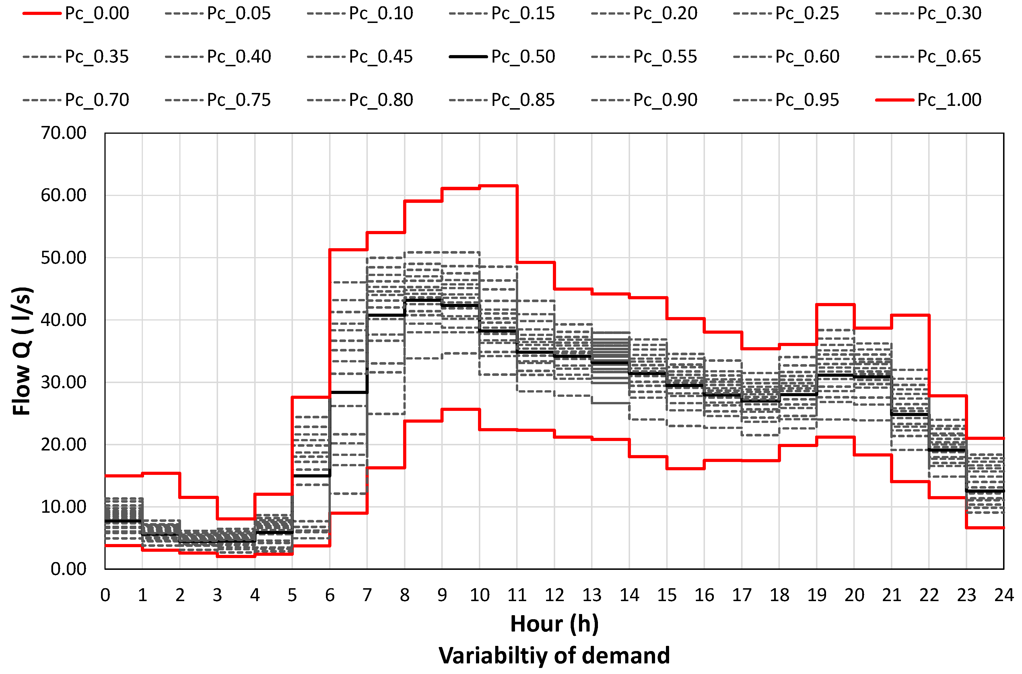
2.1.1. Demand Pattern

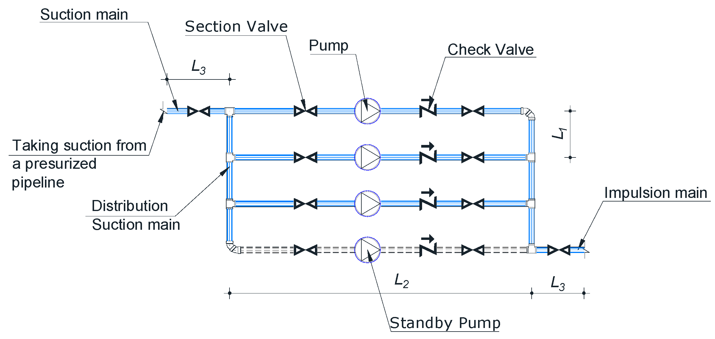
This methodology considered the variability of daily demand in the PS design. The 21 different scenarios of daily demand were derived with a probability of non-exceedance from 0 to 1 with steps of 0.05. The probability of occurrence for the scenarios with the non-exceedance probabilities 0 and 1 was 2.5%, while the probability of occurrence for the other scenarios was 5%. The scenarios were constructed as explained in the work of Briceño-León et al. [18], by using the demand data described in the work of Walski and Creaco [24].

2.1.2. PS Layout

The layout of the PS installation considered in this methodology is visualized in Figure 1. The configuration comprised a section valve situated in the suction pipeline. Then, a section valve and a check valve were installed following each branch of the pumps. Finally, these branches were integrated into a shared impulsion main with a section valve. The size of the station was determined by three pipeline lengths present in the fundamental design of the PS. The distance between each parallel pump branch corresponded to L₁, the length of the pump branches was represented by L₂, and the suction and discharge main lengths were defined by L₃.

2.1.3. Setpoint Curve

The setpoint curve is defined as the minimum head to be set in the PS, for a given network demand, in such a way that the minimum pressure head is guaranteed at the critical node. From this curve is obtained the operational points of flow and head (Q, H) of the PS that should be delivered to satisfy the required demand and pressure of the network. The equation of this curve is represented by the following form:

$$H_c=∆H+R·Q^C$$

(1)

in which ΔH and $R·Q^C$ represent the static head and energy losses produced in the network, respectively. Furthermore, c is an exponent set in such a way that the curve fits the required points of flow and head (Q, H).

2.1.4. Pump Model

The pump models are represented by the pump performance curve (Q, H) and the efficiency curve (Q, η). The forms of the typical equations to represent these curves are shown in Equations (2) and (3), as described in R. Sanks’ book [25]. In these equations, the affinity laws of a PS installation configured in parallel with several pumps were applied. Additionally, the possibility of the pumps working as VSPs was taken into account in the equations.

The constant terms of Equations (2) and (3) were obtained from a database constructed based on the manufacturer’s catalog (see Table S1 in Supplementary Material).

$$H=H_1{\alpha }^2-{\alpha }^{\left(2-B\right)}A·{\left(\frac{Q}{b}\right)}^B$$

(2)

$$\eta =E·\frac{Q}{\alpha ·b}-F·{\left(\frac{Q}{\alpha ·b}\right)}^2$$

(3)

The pump performance curve is defined by the fixed parameters A, H₁, and B in Equation (2). The pump efficiency curve is defined by the fixed parameters E and F in Equation (3). Both curves consider the rotational speed of the pump (N) and the number of pumps (b). The rotational speed of the pump is expressed as the ratio of the current rotational speed to the nominal rotational speed (α = N/N₀).

The electrical motors of the pump might range from 90% to 95%. However, in this methodology, it is considered that the mechanical power of the pump at the shaft (P_a) matches the electrical power utilized by the motor–pump assembly (P). This power encompasses both hydraulic power and the losses incurred during shaft transmission. Consequently, the overall pump assembly efficiency is established by the relation of hydraulic power to shaft power. This relation is defined by the following Equation (4):

$$\eta =\frac{P=\gamma ·Q\cdot H}{P_a=M·\omega }$$

(4)

The terms M and ω in Equation (4) are the mechanical torque of the pump and the rotational speed of the shaft, respectively, and the term γ corresponds to the specific weight of water.

In addition, the overall efficiency of the pump is corrected by applying the following formula developed by Coelho and Andrade-Campos [26] to consider the rotational speed in the pump:

$${\eta }_c=1-{\left(1-\alpha \right)}^3·\eta$$

(5)

An additional efficiency is applied to consider the correction proposed by Briceño-León et al. [13] for the affinity law, expressed as:

$${\eta }_v={\eta }_{v,0}·({\beta }_v^{k_1}-k_2·{\left(1-\alpha \right)}^{k_3})$$

(6)

The terms k₁, k₂, k₃ are constant parameters, while η_v,0 is the maximum frequency drive efficiency. Finally, P_s in Equation (6) is the consumed power of the PS, and Q_FSP and Q_VSP are the flow delivered by FSPs and VSPs, respectively.

$$P_s=\frac{\gamma ·Q_{FSP}·H}{{\eta }_c}+\frac{\gamma ·Q_{VSP}·H}{{\eta }_c·{\eta }_v}$$

(7)

2.2. Approches of PS Design

2.2.1. Classical Approach

This approach is based on LCC alone to define the PS design and comprises three stages. During the initial phase, pump models that align with the network’s hydraulic constraints are identified as viable options. Then, the required number of the viable pumps is determined. In the second stage, the five different control systems are evaluated for every one of the feasible pump models. The evaluation of the control system includes energy consumption optimization, especially for control systems integrated with VSPs. The combination of the five control systems and the feasible pump models generates several possible solutions for the PS. In the third stage, every one of the possible solutions is evaluated in economic terms (i.e., investment, operational, and maintenance costs), and the sum of these costs is the LCC. Finally, the solution with the lowest LCC is considered as the final solution.

2.2.2. Approach Based on the AHP

This second approach to PS design considers technical, economic, and environmental criteria in a comprehensive form to select the ultimate solution for the PS by applying the AHP method. The objective of the AHP method is to determine the priorities of the criteria for the PS. These priorities are obtained using the judgment of a group of experts on PS through surveys. The group of experts makes pairwise comparison of the criteria organized in a quadratic matrix to evaluate importance of each criterion against the other using a numeric scale, expressing the importance of one criterion over another. In the present work, the same modified scale as used in [18] was adopted. This scale is shown in

Table 1. Comparison of Saaty’s scale with the proposed scale.

Saaty’s Scale			Proposed Scale
NS	Ci	Cj	Ci	Cj	NS
1	50.00%	50.00%	50.00%	50.00%	1.00
2	67.67%	33.33%	55.00%	45.00%	1.22
3	75.00%	25.00%	60.00%	40.00%	1.50
4	80.00%	20.00%	65.00%	35.00%	1.86
5	83.33%	16.67%	70.00%	30.00%	2.33
6	85.71%	14.29%	75.00%	25.00%	3.00
7	87.50%	12.50%	80.00%	20.00%	4.00
8	88.89%	11.11%	85.00%	15.00%	5.67
9	90.00%	10.00%	90.00%	10.00%	9.00

Note: C_i, C_j: importance percentages (%). NS: numerical scale.

, in comparison with Saaty’s traditional scale, which has the flaw of percentage values not changing in gradual form.

Therefore, the technical, environmental, and economic criteria, along with their respective subcriteria, are assessed using a pairwise comparison matrix. This evaluation process aims to determine the priority vectors for both the criteria and subcriteria. The global priority of the subcriteria is obtained by multiplying the criteria priority vector with the subcriteria priority vector. To finalize the ranking of the subcriteria, the global priority is weighted exponentially, taking into account the inverse of the consistency index (CR) for each sub-criterion. The CR, ranging from 0 to 1, measures the consistency of the pairwise comparisons. A higher CR value indicates better consistency, approaching 1.

The subcriteria considered for the technical, economic, and environmental criteria are detailed below.

Technical Criteria

• Size: The size of the PS is a function of the number of pumps installed and the length of the pipelines in the station (see Figure 1). A higher score is assigned to this sub-criterion if the installation area is small. In this way, the highest size is assigned a score of 0 and the smallest size is assigned a score of 1. Equations (8) and (9) are used to evaluate the size of the PS.

$$L_i=f_i·{ND}_i$$

(8)

$$A=(\left(2·L_3\right)+L_2)·(b·L_1)$$

(9)

Standardized criteria to define the length of pipelines in the installation of a PS are based on the nominal diameter of the length, as established in the guidebook for pumping systems published by the Hydraulic Institute [27]. The lengths L₁, L₂, and L₃ are set proportionally to the nominal diameter of the pipes (ND_i) by using a constant factor (f_i). The sub-index i represents the type of length (L₁, L₂, or L₃).

2.

Flexibility: The flexibility of the PS is associated with the number of pumps installed, i.e., the higher the number of pumps installed, the larger the flexibility. A higher score is assigned if the number of pumps installed is large. The potential solution with the highest number of pumps (b) is assigned a score of 1 and the solution with the smallest number of pumps is assigned a score of 0.

3.

Complexity of control: This sub-criterion is related to the complexity of operation of the control system. The smaller the number of control elements in the system, the less complex the control system is considered to be. The complexity of operation is evaluated with a numeric score from 0 to 1 (see

Table 2. Numeric scores for the control system configurations.

Control System Configuration	Complexity Level	Numeric Score
1. Without CS	1	1.00
2. FSP with PC	2	0.57
3. FSP with FC	3	0.32
4. FSP-VSP with PC	4	0.15
5. FSP-VSP with FC	5	0.07

), corresponding to the highest and lowest levels of complexity, respectively, for the control systems. The scores are obtained from pairwise comparisons of the different control system strategies based on the AHP.

Economic criteria

4.

Investment cost: This includes the costs of the pumps, pipes, fittings, and control elements, as well as their installation. The investment costs are annualized considering the life cycle of the elements and the annual interest rate, and they are represented by Equation (10). A higher score is assigned to this sub-criterion if the investment cost is small. In this way, the solution with the lowest investment cost is assigned a score of 1 while 0 goes to the solution with the highest investment cost.

$$\begin{gathered} \hspace{1em}\hspace{1em}\hspace{1em}{C}_{Inv}=\left[\left(C_{PS}·b\right)·{FA}_{PS}+\left(C_{pipe}·L_T\right)·{FA}_{pipe}+\left(\sum _i^{{Acc}_i}{C}_{{Acc}_i}·N_{{Acc}_i}\right)·{FA}_{Acci} \\ +\left(\sum _j^{{RM}_j}{C}_{{RM}_j}·N_{{RM}_j}\right)·{FA}_{RMj}\right] \end{gathered}$$

(10)

Here, C_Inv represents the initial investment outlay for the PS, C_PS signifies the cost per unit of each individual pump, b denotes the count of installed pumps, FA_PS stands for the amortization factor of the pumps, C_pipe represents the cost per unit length of the pipelines, L_T indicates the overall pipeline length, and FA_pipe accounts for the pipeline amortization factor. Furthermore, C_ACCi corresponds to the cost per unit of minor station accessories such as valves and pipe connectors, while N_ACCi refers to the quantity of each minor accessory within the station. FA_ACCI represents the amortization factor for these minor accessories. Similarly, C_RMj signifies the unit cost of each control component (such as pressure switches, flow meters, pressure transducers, PLC, and VFD), N_RMj represents the number of units for each control element, and FA_RMj stands for the amortization factor of the control system devices. The amortization factor is determined using Equation (11).

$${FA}_i=\frac{T_i·{(1+T_i)}^{N_{LC}}}{{(1+T_i)}^{N_{LC}}-1}$$

(11)

Equation (11) involves variables such as FA_i, which represents the factor for amortizing the components within the PS infrastructure; T_i, denoting the yearly interest rate; and N_LC, indicating the count of years that constitute the life cycle of the components within the PS.

5.

Operational cost: This sub-criterion is related to the yearly cost (EUR) of energy consumed for operation of the PS, and it is calculated using Equation (12).

$$C_{E,year}=365\times \sum _{d=1}^{N_d}{Pr}_{DP,d}\left(\sum _{t=1}^{N_t}{P}_{T,t,d}\times ∆t\times {TE}_t\right)$$

(12)

where N_d is the number of daily demand scenarios, d corresponds to each demand scenario, the duration of the time slot is represented by Δt, Pr_DP,d is the probability of occurrence of every scenario, and TE is the electric tariff. The number 365 is used to obtain the number of days of occurrence for every demand scenario. The more economical the operational costs, the higher the rating given to this sub-criterion. Hence, the solution with the lowest operational cost is assigned a score of 1, while 0 goes to the solution with the highest operational cost.

6.

Maintenance cost: This signifies the expenses associated with performing maintenance tasks within the PS in order to uphold its optimal state. The regularity and expenses of maintenance tasks for the PS components are derived from a database, which is used to calculate the yearly maintenance expenditures. This cost is represented by Equation (13). This sub-criterion receives a higher rating when the maintenance cost is low. In this way, the solution with the lowest maintenance cost has a score of 1, while the solution with the highest maintenance cost has a score of 0.

$$\begin{gathered} \hspace{1em}\hspace{1em}\hspace{1em}\hspace{1em}{C}_{Maint}=\left[\left(\sum _i^{{APS}_i}{C}_{APSi}·F_{APSi}·b\right)+\left(C_{pipe}·F_{pipe}·L_T\right)+\left(\sum _j^{{Acc}_j}{C_{{Acc}_j}·F}_{{Acc}_j}·N_{{Acc}_j}\right) \\ +\left(\sum _k^{{RM}_k}{C_{{RM}_k}·F}_{{RM}_k}·N_{{RM}_k}\right)\right] \end{gathered}$$

(13)

In this context, C_Maint denotes the maintenance cost associated with the PS. C_APSi represents the individual cost for maintenance tasks related to the pump. F_APi signifies the yearly occurrence of maintenance activities linked to the pump. The variable ‘b’ corresponds to the count of pumps within the PS. C_pipe stands for the individual cost pertaining to maintenance tasks related to the pipelines and is expressed in units of currency (EUR/m). F_pipe represents the annual frequency at which pipeline maintenance is conducted. The parameter L_T refers to the total extent of pipeline length. C_ACCj signifies the individual cost for maintenance actions related to accessories within the PS, including valves and connectors. F_ACCj represents the yearly frequency of maintenance for each accessory. N_ACCJ represents the total quantity of units for each accessory. C_RM,j refers to the unit cost associated with maintaining control elements within the PS, such as pressure switches, flow meters, pressure transducers, PLCs, and frequency inverters. F_RMk indicates the annual frequency of maintenance for each control element, while N_RMj represents the total quantity of units for each control element. It is important to note that the maintenance tasks and their frequency for the PS components are based on the guidelines provided by the manufacturer.

Environmental criteria

7.

MEI: The minimum efficiency index (MEI) is a metric used to evaluate the energy efficiency of a pump. It is a standardized way to assess the efficiency of different pump models. A higher MEI value signifies better overall efficiency and suggests that the pump operates more efficiently across a range of flow rates. This index is established by EU regulation 547/2012 [28]. This regulation established an MEI of 0.7 as excellent, and an MEI below 0.4 as not acceptable. This sub-criterion is evaluated using a numeric scale from 0 to 1 with pairwise comparison of different MEI values based on the AHP. The obtained scores are detailed in

Table 3. Numeric scale for MEI index values.

MEI Index	Numeric Score
0.1	0.05
0.2	0.07
0.3	0.12
0.4	0.27
0.5	0.40
0.6	0.61
0.7	1.00

:

8.

CO₂ emission: This signifies the volume of CO₂ generated by the PS during its functioning. It is calculated by multiplying the energy utilized by the PS with the emission factor EF determined by El Ministerio de la Transformación Ecológica y el Reto Demográfico [29]. This sub-criterion is evaluated in terms of Kg of CO₂ in a year.

$${GHG}_{e, year}=EF\times C_{E,year}$$

(14)

A high score is assigned to this sub-criterion when the CO₂ emission is low. As a result, the solution exhibiting the lowest CO₂ emission receives a score of 1, whereas the solution associated with the highest CO₂ emission is given a score of 0.

9.

Performance of regulation: This performance (η_RS) relates the required energy at the demand node of the network to the energy delivered by the PS and is defined as the ratio of the required head of the network (H_c) to the head pumping (H) (see Equation (15)). This sub-criterion receives a high score if the regulation’s performance is good. Consequently, a score of 1 is given to the solution exhibiting the best regulatory performance, whereas a score of 0 is attributed to the solution with the worst regulatory performance.

$${\eta }_{RS,t}=\frac{H_{,t}}{H_{c,t}}$$

(15)

The second approach for PS design consists of three stages (see Figure 2. The first stage is to determine the feasible pump models for the network. In the second stage, the required number of pumps of the feasible models is determined. Then, the feasible pump models are evaluated in the five different control systems including the operating optimization. The possible solutions (N_{feasible pump models} × 5 control systems) are evaluated on the basis of the 9 subcriteria. The third stage reduces the possible solutions by identifying dominant and dominated solutions based on the 9 subcriteria. The dominant solutions are scored by using an average of each solution’s scores on every one of the 9 subcriteria weighted with their respective priority. Finally, the solution with the highest score is considered to be the ultimate solution for the PS.

The following flowchart (Figure 2) describes the different stages of the proposed methodology: the input of required data, the determination of the feasible pump models, and finally, the assessment of the potential solution and the selection of the ultimate solution.

2.3. Sensitibity Analysis

The obtained solutions for the PS design mainly depended on the hydraulic characteristics of the network (i.e., setpoint curve, demand) and on the electricity price and annual interest rate of amortization. The sensitivity analysis consisted of testing and evaluating the solutions obtained with the classical approach of PS design and with the approach based on AHP against different scenarios of operation. The different scenarios used for the sensitivity analysis were obtained by applying variations in the average demand (Q_m), pipeline lengths of the PS layout (L_i), hydraulic parameters of the setpoint curve (ΔH, R), electricity tariff prices (TE), and annual amortization interest rate (T_i). The objective of the sensitivity analysis was to determine the operational limits of these network parameters without changing the final solution of PS design. Therefore, gradual increases and decreases in each of these network parameters were performed iteratively until the final solutions for the two PS design approaches changed. The increment and decrement intervals were considered to be 0.5%. Finally, this analysis allowed evaluation of the robustness and reliability of the pumping station designs based on the AHP method versus the classical design approach.

3. Case Study

This work considered a hypothetical closed WDN as the case study for performing the sensitivity analysis on the two approaches of PS design. The hydraulic characteristics of this WDN are shown in

Table 4. Hydraulic parameters of the WDN.

Data	Qm (L/s)	ΔH (m)	R	c
	25.00	29.50	0.0109	1.95
$H_c=29.50+0.0109\times Q^{1.95}$

. This table includes the mean yearly demand of the network (Q_m = 25.00 L/s) and the parameters of the setpoint curve (ΔH, R, c).

There were 67 pump models that were evaluated in the two approaches to obtain the most suitable solution for each approach. The data for the pump models included the hydraulic parameters of the performance and efficiency curves as well as the cost of each model.

On the other hand, the velocity design considered for the sizing of the diameter of the pipelines in the PS layout was (V = 2.0 m/s). The multiplying factors for the pipe nominal diameters for the dimensioning of the pipeline lengths were considered as follows: N₁ = 20, N₂ = 40, and N₃ = 20. Finally, the maximum number of installed pumps (b_max) allowed for the PS design was 10.

The 21 daily demand scenarios considered for this WDN are shown in Figure 3, where every scenario is characterized by its probability of non-exceedance (P_c) from 0 to 1.

The electric tariff used in this case study corresponded to the average of the hourly electric tariff patterns over the last 5 years in Spain and the average of the daily electric tariff price. These data were obtained from a database provided by an energy supply company. Figure 4 shows the pattern of average hourly variability in electric tariffs for each year, with their respective averages of daily electric tariff prices and the overall averages of hourly variability in the last five years. Figure 5, on the other hand, shows the daily variability in electricity tariff prices from January of 2018 to December of 2022.

As can be seen in Figure 4 and Figure 5, the hourly variability in the electricity tariff is slight, and the change in the patterns was minimal in each year and would not have a significant effect on the design of a PS. However, when the daily variability of the electric tariff price is analyzed, it undergoes drastic changes through the years, and it could affect the selected solution for the PS design. Therefore, it is important to perform a sensitivity analysis on the approaches for PS design when the electricity price changes. For this reason, the average daily electric tariff price in every year with the overall pattern of average hourly variability were evaluated in both approaches of PS design to determine how changes in the daily electricity tariff affects the ultimate solution for the PS design.

3.1. Results

First, the classical PS design approach and the PS design based on the AHP were evaluated with the original data of the WDN. The ultimate solutions for both approaches are shown in

Table 5. Ultimate solutions of PS approaches with original data of the WDN.

Approaches		First Approach	Second Approach
Pump Characteristics	Pump Model	32	64
	Q0 (L/s)	22.71	16.97
	H0 (m)	61.06	61.52
	ηmax (%)	61%	83%
Tec. Aspects	C1 (m2)	151.20	140.80
	C2	0 FSP–3 VSP	1 FSP–3 VSP
	C3	5	5
Eco. Aspects	C4 (EUR/year)	5355.78	12,778.24
	C5 (EUR/year)	13,079.49	9460.92
	C6 (EUR/year)	1193.21	1462.31
Env. Aspects	C7	0.10	0.70
	C8 Kg CO2	57,041.02	41,208.60
	C9 (%)	100%	100%
Life Cycle Cost (EUR/year)		19,628.48	23,701.47

Note: C1: PS size; C2: control system; C3: number of pumps; C4: investment cost; C5: operational cost; C6: maintenance cost; C7: MEI; C8: GHG emission; C9: regulation performance.

. This figure contains the BEP of the pump models of the ultimate solutions and the values for the nine subcriteria considered for the design in every approach.

The ultimate solutions obtained with the two approaches were different in the characteristics of the pump model. The main differences in the pump models were in the flow capacity, which was greater in the second approach, leading to different scores for the various subcriteria. One of the highlighted subcriteria was that the solution in approach 2 had better flexibility than approach 1 with a greater number of pumps in approach 2 than in approach 1. In addition, the MEI of the solution in approach 2 was better than approach 1. Therefore, it was implied that operational costs and GHG emissions in approach 2 would be lower than in approach 1. The complexity of operation, maintenance costs, and performance of regulation were, however, very similar in both approaches. On the other hand, investment cost and LCC were greater in approach 2 than in approach 1.

In summary, the selection of the ultimate solution in approach 1 depended only on LCC, while the selection of the ultimate solution in approach 2 depended on several factors related to technical, economic, and environmental criteria. Hence, the ultimate solution in approach 2 provided better performance in most of the subcriteria than the ultimate solution in approach 1. In addition, the consideration of technical, economic, and environmental criteria in PS design could imply that the ultimate solution in approach 2 would be more robust than the ultimate solution obtained in approach 1, when tackling different operational scenarios that could occur in a WDN in terms of modified demand, setpoint curve, or electricity tariffs.

Both approaches were evaluated with different interest rate of amortization factors (T_i), by increasing and decreasing them with a step of 0.5% with respect to the original interest rate (T_i) of the case study until the ultimate solution in every approach was different from the original case study, to determine the sensitivity of this data for selecting the ultimate solution in both approaches. The obtained results of this sensitivity analysis are shown in

Table 6. Sensitivity analysis with interest rate in both approaches to PS design.

Approaches		Ti + 50% = 4.5%	Ti − 50% = 1.5%	Ti + 50% = 4.5%	Ti − 50% = 1.5%
		Approach 1	Approach 1	Approach 2	Approach 2
Pump Characteristics	PumpModel	32	32	64	64
	Q0 (L/s)	22.71	22.71	16.97	16.97
	H0 (m)	61.06	61.06	61.52	61.52
	ηmax (%)	61%	61%	83%	83%
Tec. Aspects	C1 (m2)	151.20	151.20	140.80	140.80
	C2	0 FSP–3 VSP	0 FSP–3 VSP	1 FSP–3 VSP	1 FSP–3 VSP
	C3	5	5	5	5
Eco. Aspects	C4 (EUR/year)	5876.52	4866.67	13,928.41	11,688.22
	C5 (EUR/year)	13,079.49	13,079.49	9460.92	9460.92
	C6 (EUR/year)	1193.21	1137.46	1462.31	1462.31
Env. Aspects	C7	0.10	0.10	0.70	0.70
	C8 Kg CO2	57,041.02	57,041.02	41,208.60	41,208.60
	C9 (%)	100%	100%	100%	100%
Life Cycle Cost (EUR/year)		20,197.24	19,187.39	24,851.63	22,611.45

Note: C1: PS size; C2: control system; C3: number of pumps; C4: investment cost; C5: operational cost; C6: maintenance cost; C7: MEI; C8: GHG emission; C9: regulation performance.

. The obtained results in Table 6 demonstrated that the ultimate solutions in both approaches were not sensitive to the interest rate (T_i), even though the interest rate could change drastically +/−50% compared to the original interest rate. The only changes in the ultimate solutions for the two approaches produced by increasing or decreasing the interest rate were in the investment costs and LCC. The characteristics of the pump models in the ultimate solutions and the values for the other subcriteria in both approaches were identical to the original results of the case study.

The sensitivity analysis of the mean demand (Q_m) in both approaches is illustrated in

Table 7. Sensitivity analysis with the mean flow in the PS design approach based on LCC minimization.

Approaches		Qm_max = Qm + 1% (25.25 L/s)	Qm + 2% (25.5 L/s)	Qm_max = Qm − 3% (24.25 L/s)	Qm − 4% (24.0 L/s)
		Approach 1	Approach 1	Approach 1	Approach 1
Pump Characteristics	Pump Model	32	33	32	31
	Q0 (L/s)	22.71	24.32	22.71	19.50
	H0 (m)	61.06	78.73	61.06	50.43
	ηmax (%)	61%	61%	61%	70%
Tec. Aspects	C1 (m2)	151.20	151.20	151.20	158.40
	C2	0 FSP–3 VSP	0 FSP–3 VSP	1 FSP–2 VSP	2 FSP–3 VSP
	C3	5	5	5	5
Eco. Aspects	C4 (EUR/year)	5355.78	6604.70	5152.23	6328.61
	C5 (EUR/year)	13,258.22	13,320.51	12,552.96	10,594.24
	C6 (EUR/year)	1193.21	1193.21	1170.78	1739.98
Env. Aspects	C7	0.10	0.11	0.10	0.10
	C8 Kg CO2	57,814.90	58,075.52	54,760.90	46,194.04
	C9 (%)	100%	100%	100%	100%
Life Cycle Cost (EUR/year)		19,807.21	21,118.41	18,875.97	18,662.84

Note: C1: PS size; C2: control system; C3: number of pumps; C4: investment cost; C5: operational cost; C6: maintenance cost; C7: MEI; C8: GHG emission; C9: regulation performance.

and

Table 8. Sensitivity analysis with the mean flow in the PS design approach based on AHP with technical, economic, and environmental criteria.

Approaches		Qm_max = Qm + 2% (25.50 L/s)	Qm + 3% (25.75 L/s)	Qm_min = Qm − 2% (24.50 L/s)	Qm − 3% (24.25 L/s)
		Approach 2	Approach 2	Approach 2	Approach 2
Pump Characteristics	Pump Model	64	33	64	44
	Q0 (L/s)	16.97	24.32	16.97	19.50
	H0 (m)	61.52	78.73	61.52	50.43
	ηmax (%)	83%	61%	83%	70%
Tec. Aspects	C1 (m2)	140.80	140.80	140.80	144.00
	C2	1 FSP–3 VSP	0 FSP–3 VSP	1 FSP–3 VSP	6 FSP–0 VSP
	C3	5	5	5	3
Eco. Aspects	C4 (EUR/year)	12,778.24	8376.14	12,778.24	9542.55
	C5 (EUR/year)	9732.85	13,501.42	9193.33	14,782.81
	C6 (EUR/year)	1462.31	1210.36	1462.31	1918.87
Env. Aspects	C7	0.70	0.12	0.70	0.70
	C8 Kg CO2	42,387.25	58,858.99	40,048.68	64,669.36
	C9 (%)	100%	100%	100%	71%
Life Cycle Cost (EUR/year)		23,973.41	23,087.92	23,433.88	26,244.24

Note: C1: PS size; C2: control system; C3: number of pumps; C4: investment cost; C5: operational cost; C6: maintenance cost; C7: MEI; C8: GHG emission; C9: regulation performance.

. The mean demand (Q_m) of the original case study was incremented and decremented with a step of 1% until the ultimate solution in every PS design approach was different.

The maximum and minimum limits of the allowed mean demand range (Q_{m_max,} Q_{m_min}) in the first approach was 25.25 L/s and 24.25 L/s, respectively. The ultimate solution of the original case study was valid with a range of mean demand (Q_m) from 24.25 L/s to 25.25 L/s with the same pump model and same control system strategy, as can observed in Table 7. A variation in the mean demand (Q_m) of the case study generated different values in the subcriteria, especially for investment costs, operational costs, GHG emissions, and LCC in the ultimate solutions. However, the ultimate solution remained the same. In contrast, when the mean demand (Q_m) was outside the range 24.25 L/s to 25.25 L/s, the ultimate solution of the first approach was different from the ultimate solution of the original case study, in terms of pump model, control system, and the values for the subcriteria.

The minimum and maximum limits of mean demand in the second approach were Q_{m_,min} = 24.50 L/s and Q_{m_max} = 25.50 L/s, respectively. The ultimate solution of the second approach in this range of mean demand (Q_m = 24.50 L/s to 25.50 L/s) was the same as the ultimate solution of the original case study with the same pump model and control system strategy, but with different subcriteria values, as can observed in Table 8. For example, operational costs, GHG emission, and the LCC of the ultimate solution changed in accordance with mean demand (Q_m). On the other hand, if the mean demand (Q_m) of the WDN was outside of that range (24.50 L/s to 25.50 L/s), the ultimate solution of the second approach was different from the ultimate solution of the original case study, involving a different pump model and different values for the subcriteria.

The sensitivity analysis of the setpoint curve for both PS design approaches included the parameters ΔH and R (see Section 2.1.3). First, the sensitivity analysis of the static head (ΔH) was performed with an iterative process by increasing and decreasing the original static head (ΔH) of the WDN with a step 1% until the ultimate solution in every approach was different from the original ultimate solution. This analysis allowed determination of the range of static head (ΔH) where the ultimate solutions of the PS design approaches were not affected by changes in the static head (ΔH).

Table 9. Sensitivity analysis with the parameter (ΔH) of the setpoint curve for the first PS design approach.

Approaches		ΔHmax = ΔH + 5% (30.98 m)	ΔH + 6% (31.27 m)	ΔHmin = ΔH − 8% (27.14 m)	ΔH − 9% (26.85 m)
		Approach 1	Approach 1	Approach 1	Approach 1
Pump Characteristics	Pump Model	32	33	32	31
	Q0 (L/s)	22.71	24.32	22.71	19.50
	H0 (m)	61.06	78.73	61.06	50.43
	ηmax (%)	61%	61%	61%	70%
Tec. Aspects	C1 (m2)	151.20	151.20	151.20	158.40
	C2	0 FSP–3 VSP	0 FSP–3 VSP	1 FSP–2 VSP	2 FSP–3 VSP
	C3	5	5	5	5
Eco. Aspects	C4 (EUR/year)	5355.78	6604.70	5355.78	6328.61
	C5 (EUR/year)	13,549.89	13,494.90	12,334.95	10,471.42
	C6 (EUR/year)	1193.21	1193.21	1193.21	1739.98
Env. Aspects	C7	0.10	0.11	0.10	0.10
	C8 Kg CO2	59,104.26	58,860.22	53,775.66	45,625.47
	C9 (%)	100%	100%	100%	100%
Life Cycle Cost (EUR/year)		20,098.88	21,292.80	18,883.94	18,540.02

Note: C1: PS size; C2: control system; C3: number of pumps; C4: investment cost; C5: operational cost; C6: maintenance cost; C7: MEI; C8: GHG emission; C9: regulation performance.

and

Table 10. Sensitivity analysis with the parameter (ΔH) of the setpoint curve for the second PS design approach.

Approaches		ΔHmax = ΔH + 7% (31.57 m)	ΔH + 8% (31.27 m)	ΔHmin = ΔH − 21% (23.31 m)	ΔH − 22% (23.01 m)
		Approach 2	Approach 2	Approach 2	Approach 2
Pump Characteristics	Pump Model	64	32	64	31
	Q0 (L/s)	16.97	22.71	16.97	19.35
	H0 (m)	61.52	61.06	61.52	50.43
	ηmax (%)	83%	61%	83%	70%
Tec. Aspects	C1 (m2)	140.80	140.80	140.80	140.80
	C2	1 FSP–3 VSP	1 FSP–3 VSP	1 FSP–3 VSP	1 FSP–3 VSP
	C3	5	5	5	5
Eco. Aspects	C4 (EUR/year)	12,778.24	6261.77	12,778.24	5447.80
	C5 (EUR/year)	9922.35	13,839.98	8092.24	9421.28
	C6 (EUR/year)	1462.31	1462.31	1462.31	1462.31
Env. Aspects	C7	0.70	0.10	0.70	0.19
	C8 Kg CO2	43,226.87	60,376.79	35,223.68	41,029.30
	C9 (%)	100%	100%	100%	100%
Life Cycle Cost (EUR/year)		24,162.90	21,564.06	22,814.32	16,331.39

Note: C1: PS size; C2: control system; C3: number of pumps; C4: investment cost; C5: operational cost; C6: maintenance cost; C7: MEI; C8: GHG emission; C9: regulation performance.

contain the ultimate solutions and their values for the subcriteria for the maximum and minimum limits of the static head (ΔH) range obtained from the sensitivity analysis for the first and second approaches, respectively. In addition, these tables present the obtained ultimate solutions for each approach with scenarios of the static head (ΔH) that were outside of the maximum and minimum limits.

The range of the static head (ΔH) of the WDN, where the ultimate solution of the first PS design approach was not affected, was from 27.14 m to 30.98 m, as is observed in Table 10. The ultimate solutions of the first approach when the static head (ΔH) was at the maximum limit (ΔH = 30.98 m) and at the minimum limit (ΔH = 30.98 m) were similar and featured the same pump model, control system strategy, and values for most of subcriteria. The only differences between these ultimate solutions were in the obtained values for the subcriteria operational costs, GHG emissions, and LCC. The values of these subcriteria changed in accordance with the changes in the static head (ΔH) of the WDN. On the other hand, when the static head (ΔH) was outside the range (ΔH_max < ΔH < ΔH_min), the ultimate solutions were different from the ultimate solution of the original case study and featured different pump models, control system strategies, and values for the subcriteria, as reported in Table 9.

Table 10 shows that the range of the static head (ΔH) in the WDN where altering ΔH in the setpoint curve did not impact the ultimate solution of the second PS design approach spanned from 23.31 m to 31.57 m (much wider than the range obtained for the first approach). The second approach yielded similar ultimate solutions when the static head (ΔH) reached its maximum limit (ΔH = 31.57 m) and minimum limit (ΔH = 23.31 m). These solutions employed the same pump model and control system strategy, and had matching values for most subcriteria. The disparities between these ultimate solutions lay only in the operational costs and GHG emissions subcriteria and, of course, the LCC. As the static head (ΔH) of the WDN increased or decreased, the subcriteria values changed accordingly. Conversely, when the static head (ΔH) fell outside the designated range (ΔH_max < ΔH < ΔH_min), the ultimate solutions differed from the original case study. These divergent solutions involved different pump models, control system strategies, and distinct subcriteria values, as reported in Table 10.

The second parameter considered in the sensitivity analysis of the setpoint curve in both design approaches for PSs was the losses generated in the system (R). This sensitivity involved an iterative process, where the original losses (R) of the WDN were increased or decreased by a step of 1%. This process continued until the ultimate solution for each approach differed from the ultimate solution of the original case study. By conducting this analysis, it was possible to identify the permitted range of losses (R) where the ultimate solutions of the PS design approaches were not affected by the variation in the losses (R) in the setpoint curve.

Table 11. Sensitivity analysis with the losses (R) of the setpoint curve in the first PS design approach.

Approaches		Rmax = R + 5% (0.0114)	R + 6% (0.0116)	Rmin = R − 7% (0.0101)	R − 8% (0.0100)
		Approach 1	Approach 1	Approach 1	Approach 1
Pump Characteristics	Pump Model	32	33	32	31
	Q0 (L/s)	22.71	24.32	22.71	19.35
	H0 (m)	61.06	78.73	61.06	50.43
	ηmax (%)	61%	61%	61%	70%
Tec. Aspects	C1 (m2)	151.20	151.20	151.20	158.40
	C2	0 FSP–3 VSP	0 FSP–3 VSP	1 FSP–2 VSP	2 FSP–3 VSP
	C3	5	5	5	5
Eco. Aspects	C4 (EUR/year)	5355.78	6604.70	5355.78	6328.61
	C5 (EUR/year)	13,233.72	13,139.54	12,864.50	10,990.73
	C6 (EUR/year)	1193.21	1193.21	1193.21	1739.98
Env. Aspects	C7	0.10	0.11	0.10	0.10
	C8 Kg CO2	57,707.91	57,290.64	56,111.42	47,912.66
	C9 (%)	100%	100%	100%	100%
Life Cycle Cost (EUR/year)		19,782.71	20,937.44	19,413.48	19,059.32

Note: C1: PS size; C2: control system; C3: number of pumps; C4: investment cost; C5: operational cost; C6: maintenance cost; C7: MEI; C8: GHG emission; C9: regulation performance.

and

Table 12. Sensitivity analysis with the losses (R) of the setpoint curve in the second PS design approach.

Approaches		Rmax = R + 6% (0.0116)	R + 7% (0.0117)	Rmin = R − 19% (0.0088)	R − 20% (0.0087)
		Approach 2	Approach 2	Approach 2	Approach 2
Pump Characteristics	Pump Model	64	32	64	31
	Q0 (L/s)	16.97	22.71	16.97	19.35
	H0 (m)	61.52	61.06	61.52	50.43
	ηmax (%)	83%	61%	83%	70%
Tec. Aspects	C1 (m2)	140.80	140.80	140.80	140.80
	C2	1 FSP–3 VSP	1 FSP–3 VSP	1 FSP–3 VSP	1 FSP–3 VSP
	C3	5	5	5	5
Eco. Aspects	C4 (EUR/year)	12,778.24	6261.77	12,778.24	5447.80
	C5 (EUR/year)	9595.57	13,301.39	9035.25	10,640.50
	C6 (EUR/year)	1462.31	1462.31	1462.31	1462.31
Env. Aspects	C7	0.70	0.10	0.70	0.19
	C8 Kg CO2	41,790.42	58,000.73	39,369.32	46,400.27
	C9 (%)	100%	100%	100%	100%
Life Cycle Cost (EUR/year)		23,836.13	21,025.46	23,757.32	17,550.61

Note: C1: PS size; C2: control system; C3: number of pumps; C4: investment cost; C5: operational cost; C6: maintenance cost; C7: MEI; C8: GHG emission; C9: regulation performance.

present the ultimate solutions and their corresponding values for the subcriteria. These values were obtained from the sensitivity analysis for the maximum and minimum limits of the losses range (R_max, R_min), using the first and second approaches, respectively. Additionally, these tables display the ultimate solutions obtained by each approach when scenarios with values of losses (R) exceeding the maximum and minimum limits of the range were considered.

The sensitivity analysis of losses (R) in the WDN of the first PS design approach (see Table 11) determined that the permissible range of losses where the ultimate solution was not affected was from 1.01 × 10⁻³ to 1.14 × 10⁻³. When losses (R) reached these maximum and minimum limits (R_max, R_min), the ultimate solutions of the first approach were the same as the ultimate solution with the original data of the WDN. In fact, these ultimate solutions yielded the same values for the subcriteria as the ultimate solution of the original case study, except for the subcriteria operational costs and GHG emissions and the LCC. The values of these subcriteria in the ultimate solution were in accordance with the losses in the WDN. On the contrary, when losses (R) reached values above or below the maximum and minimum of the permissible range (e.g., R_max = 1.16 × 10⁻³ and R_min = 1.10 × 10⁻³), the ultimate solutions of the first approach were different from the ultimate solution in the original case study, including different pump models and different subcriteria values.

The sensitivity analysis conducted on the losses (R) of the water distribution network (WDN) using the second PS design approach (refer to Table 12) revealed that the allowable range of losses, where the ultimate solution remained unaffected, spanned from 0.80 × 10⁻³ to 1.16 × 10⁻³ (wider than the range obtained for the first design approach). When the losses (R) fell within these upper and lower limits (0.80 × 10⁻³ < R < 1.16 × 10⁻³), the ultimate solutions obtained using the second approach aligned with the ultimate solution derived from the original WDN data. In fact, the only differences between these ultimate solutions and the original ultimate solution were in the operational costs, GHG emission, and LCC. The values of these subcriteria for the ultimate solution were in accordance with the losses (R) in the WDN. Conversely, when the losses (R) exceeded or fell below the permissible range (for instance, with values of R = 1.16 × 10⁻³ and R = 1.10 × 10⁻³), the ultimate solutions obtained using the second approach differed from the ultimate solution in the original case study, involving different pump models and consequently different subcriteria values.

Two scenarios of the average annual tariff price were evaluated for each of the PS design approaches for the sensitivity analysis of the electricity tariff. The first scenario corresponded to the minimum price of the average annual tariff over the last 5 years (TE = EUR 0.034) and the second scenario to the maximum price of the average annual tariff of the last 5 years (TE = EUR 0.17).

The ultimate solutions with their respective subcriteria values for both PS design approaches with the maximum and minimum average electric tariff in the last 5 years are shown in

Table 13. Sensitivity analysis with the electric tariff in both PS design approaches.

Approaches		TEmax = EUR 0.17	TEmin = EUR 0.034	TEmax = EUR 0.17	TEmin = EUR 0.034
		Approach 1	Approach 1	Approach 2	Approach 2
Pump Characteristics	Pump Model	31	32	64	64
	Q0 (L/s)	19.35	22.71	16.97	16.97
	H0 (m)	50.43	61.06	61.52	61.52
	ηmax (%)	70%	61%	83%	83%
Tec. Aspects	C1 (m2)	140.80	151.20	140.80	140.80
	C2	1 FSP–3 VSP	0 FSP–3 VSP	1 FSP–3 VSP	1 FSP–3 VSP
	C3	5	5	5	5
Eco. Aspects	C4 (EUR/year)	12,778.24	5355.78	12,778.24	12,778.24
	C5 (EUR/year)	3875.56	5357.86	19,377.78	9460.92
	C6 (EUR/year)	1462.31	1193.21	1462.31	1397.98
Env. Aspects	C7	0.70	0.10	0.70	0.70
	C8 Kg CO2	41,208.60	57,041.02	41,208.60	41,208.60
	C9 (%)	100%	100%	100%	100%
Life Cycle Cost (EUR/year)		11,906.85	33,233.21	33,618.33	18,116.11

Note: C1: PS size; C2: control system; C3: number of pumps; C4: investment cost; C5: operational cost; C6: maintenance cost; C7: MEI; C8: GHG emission; C9: regulation performance.

.

The ultimate solution of the first approach with the minimum average electric tariff (TE_min = EUR 0.034) led to the same pump model and control system as the ultimate solution in the original case study. In this case, the change of the average annual electric tariff only affected the operational costs and LCC. However, when the electric tariff reached the maximum average annual electric tariff (TE_max = EUR 0.17) in the first approach, the ultimate solution was different from the ultimate solution in the original case study, as it featured a different pump model and consequently different subcriteria values. In this case, the ultimate solution of the first approach was affected significantly when the electric tariff reached the maximum average annual tariff over the last 5 years.

The ultimate solutions of the second PS design approach obtained with the lowest and highest average annual electric tariffs in the case study (TE_min = EUR 0.034 and TE_max = EUR 0.17), resulted in the adoption of the same pump model and control system as the ultimate solution in the original case study. In the second approach, the alteration of the electric tariff did not affect the ultimate solution of the PS design. The electric tariff solely impacted the operational costs and LCC.

3.2. Discussion

A PS design depends on several variables in a WDN, such as mean demand (Q_m), the setpoint curve (e.g., static head (ΔH), losses (R)), and the electric tariff (TE). In addition, other variables influence PS design, such as the interest rate (T_i) of the amortization factor. However, the effects that these variables have in PS design are different. Moreover, another important point is that these variables affect the outcome of PS design differently depending on the approach considered in the design. In this study, two approaches to PS design were considered. The first approach, the classic approach, was based on the minimization of LCC, while the second approach was based on the AHP and considered technical, economic, and environmental criteria. Therefore, a sensitivity analysis of the different meaningful variables of PS design was carried out for both design approaches. The most salient results of the sensitivity analyses performed on each PS design approach are discussed below.

The obtained results from the sensitivity analysis of the interest rate (T_i) of amortization factor in both PS design approaches (see Table 6) showed that the ultimate solutions of both Ps design approaches were not sensitive to alteration of the interest rate (T_i). The only effects produced in the ultimate solution in each design approach by a change in the interest rate (T_i) were in the investment cost and the LCC as the interest rate (T_i) varied. However, the ultimate solution for each approach was the same regardless of the interest rate (T_i).

The sensitivity analysis with the mean flow (Q_m) in approaches 1 and 2 (referred to in Table 7 and Table 8) demonstrated that the selection of the ultimate solution in both approaches was very sensitive to a fluctuation in the mean flow (Q_m). The permitted flow range in the first design approach, where the ultimate solution of the original case study was not altered, was from 24.25 L/s to 25.25 L/s. Hence, the range of mean flow variations (ΔQ_m) that would not affect the ultimate solution in the first approach was 1 L/s. Similarly, the range of the mean flow fluctuations (ΔQ_m) in the second design approach that would not alter the ultimate solution of the original case study was 1 L/s, with a range from 24.5 L/s to 25.5 L/s. Therefore, both PS design approaches have the same sensitive to fluctuation in the mean flow (Q_m) in the WDN.

The evaluation of variation in the static head (ΔH) in the setpoint curve of the ultimate solutions for both PS design approaches (refer to Table 9 and Table 10) determined that the selection of the ultimate solution was more sensitive to a fluctuation in the static head (ΔH) in the first design approach than in the second approach. The tolerable range of static head (ΔH) that would not affect the ultimate solution of the first approach was from 27.14 m to 30.48 m, with an amplitude of 3.34 m. The allowable span of static head (ΔH) within which the ultimate solution of the second approach remained valid extended further, compared to the first approach, ranging from 23.31 m to 31.57 m, that is, for 8.26 m. The fact that the first approach only considered the LCC for selecting the ultimate solution made it more sensitive to varying the static head (ΔH) of the setpoint curve. In addition, the static head (ΔH) fluctuation mainly affected operational cost, GHG emission, and LCC in that solution for the PS. On the contrary, the second approach considered technical, economic, and environmental criteria based on the AHP to select the ultimate solution. Therefore, this multi-criteria analysis in the design made the solution more robust when facing variation in the static head (ΔH) of the setpoint curve.

In the same way, the analysis of variation in losses (R) in the setpoint curve revealed that the sensitivity to fluctuations differed between the ultimate solutions in the two PS design approaches (refer to Table 11 and Table 12). In the first approach, the acceptable range of losses (R) where there was no effect on the selection of the ultimate solution was from 1.01 × 10⁻³ to 1.14 × 10⁻³, with an amplitude of 0.13 × 10⁻³. The second approach had a wider range, from 0.80 × 10⁻³ to 1.16 × 10⁻³, with an interval of 0.36 × 10⁻³. The variation in losses (R) in the setpoint curve primarily impacted operational costs, GHG emissions, and LCC in the ultimate solution of the PS. The first approach solely considered LCC for ultimate solution selection, making it more susceptible to changes in losses (R) in the setpoint curve. Conversely, the second approach incorporated technical, economic, and environmental criteria using the AHP, resulting in a more robust solution when losses varied in the setpoint curve.

The sensitivity analysis with the alteration of the electric tariff (TE) for the selection of the ultimate solutions showed important differences in the two PS design approaches (refer to Table 13). On the one hand, the solution obtained in the first approach was affected when the electricity tariff reached its maximum annual average value from the last 5 years. On the other hand, the second approach’s solution was not affected by variation in the electricity tariff (TE), even when it reached the maximum and minimum annual average values from the last 5 years. In general, a change in the electric tariff affected the operational costs of the solution in both PS design approaches. However, only the ultimate solution of the first PS approach was sensitive to variation in the electric tariff. This approach relied only on LCC to determine the PS solution, and this made the selection of the solution sensitive to significant changes in the annual electricity tariff. On the contrary, the multi-criteria analysis of technical, economic, and environmental aspects based on the AHP to define the ultimate PS solution in the second approach made that solution dependent on multiple factors. Therefore, the solution in the second approach was robust and remained unchanged by variations in the annual electricity tariff.

4. Conclusions

The conclusions drawn from the sensitivity analysis and the tolerance ranges of various variables in the two approaches to PS design were as follows:

Interest Rate (Ti):

• The tolerance range for the variation in amortization interest rate was undefined because the amortization rate did not affect the selection of the ultimate solution in either PS design approach (see Table 8).
• Variations in the amortization interest rate impacted both pumping station design approaches in the same way. These mainly affected the investment costs and, consequently, the LCC in the final solutions of both approaches. However, the pump model of the ultimate solutions in both approaches remained unchanged.

Mean Flow (Q_m):

• The allowable range of mean flow (Q_m) variation that did not affect the ultimate solution was similar for both approaches with the same length of the tolerance range, as is visualized in Table 9 and Table 10.
• Variations in the mean flow (Q_m) within the tolerance range (Q_min < Q_m < Q_max) had an impact on operational costs, GHG emissions, and LCC, while maintaining the ultimate solution of the original case study in both approaches.
• Fluctuations in the average flow rate outside the tolerance range generated significant effects on the selection of the final solution in both design approaches. In the first approach, with the flow variation outside the tolerance range, the final solution was changed mainly in the pump model and its flow capacity, while in the second approach, the final solution was changed in the pump model and its flow capacity, the number of pumps, and the control strategy.

Static Head (ΔH) and Losses (R):

• The tolerance range for static head (ΔH) and losses (R) in the second approach was wider than in the first approach (see Table 11 and Table 12).
• Fluctuations in static head (ΔH) and losses (R) had a greater impact on the first design approach compared to the second approach.
• Variations in static head (ΔH) and losses (R) within the tolerance range in the setpoint curve primarily impacted operational costs, greenhouse gas (GHG) emissions, and the LCC of the ultimate solutions in both design approaches. However, the first approach, which considered only LCC, was more susceptible to changes in losses, while the second approach, incorporating multi-criteria analysis including technical, economic, and environmental factors, was more robust facing variations in the variables of static head (ΔH) and losses (R).
• On the other hand, when the variations of the static head (ΔH) and losses (R) were outside the tolerance range, the main impact on the selected solutions in both approaches was a change in the pump model, with different flow and pumping head capacity, from that of the ultimate solution in the original case study.

Electric Tariff (TE):

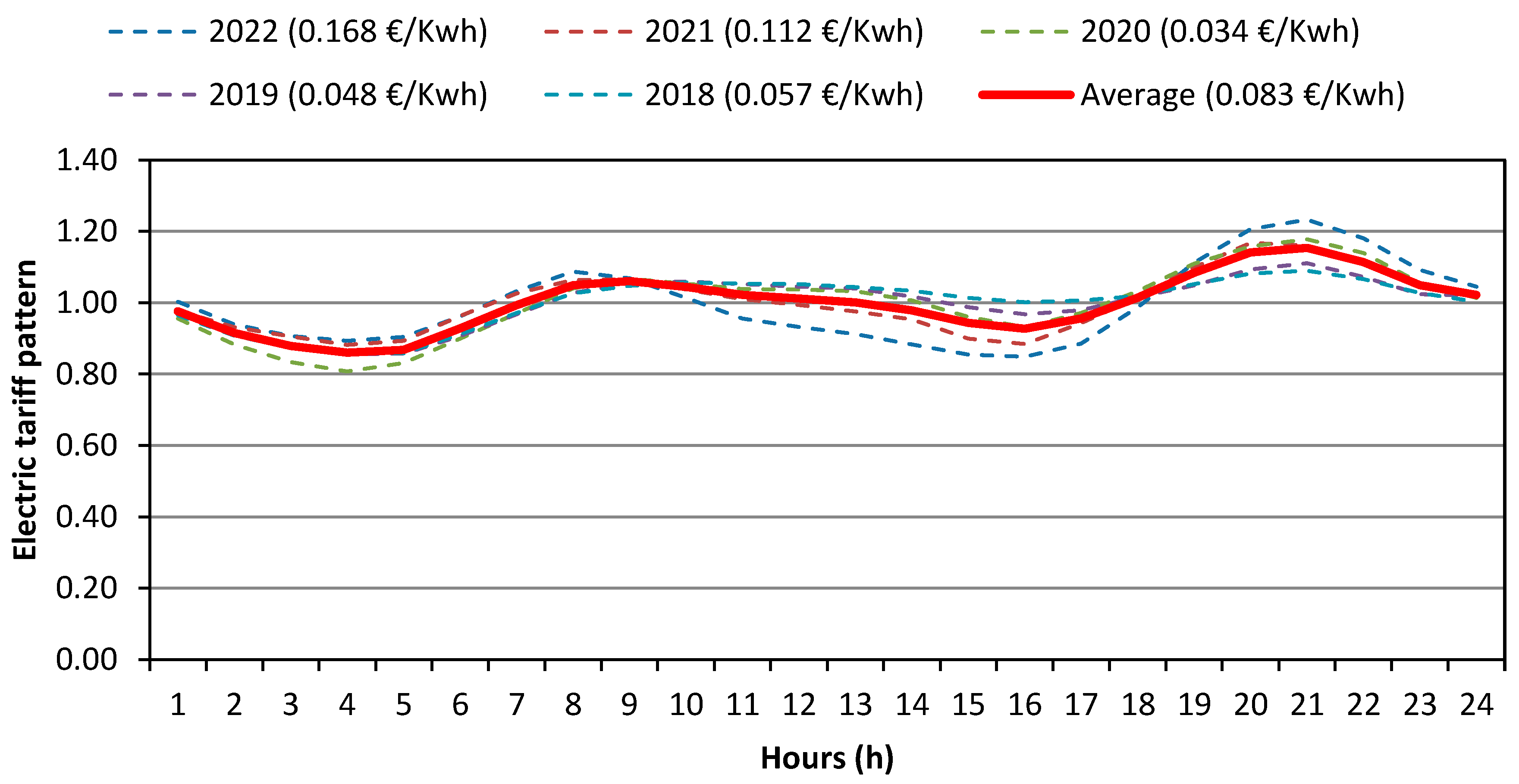
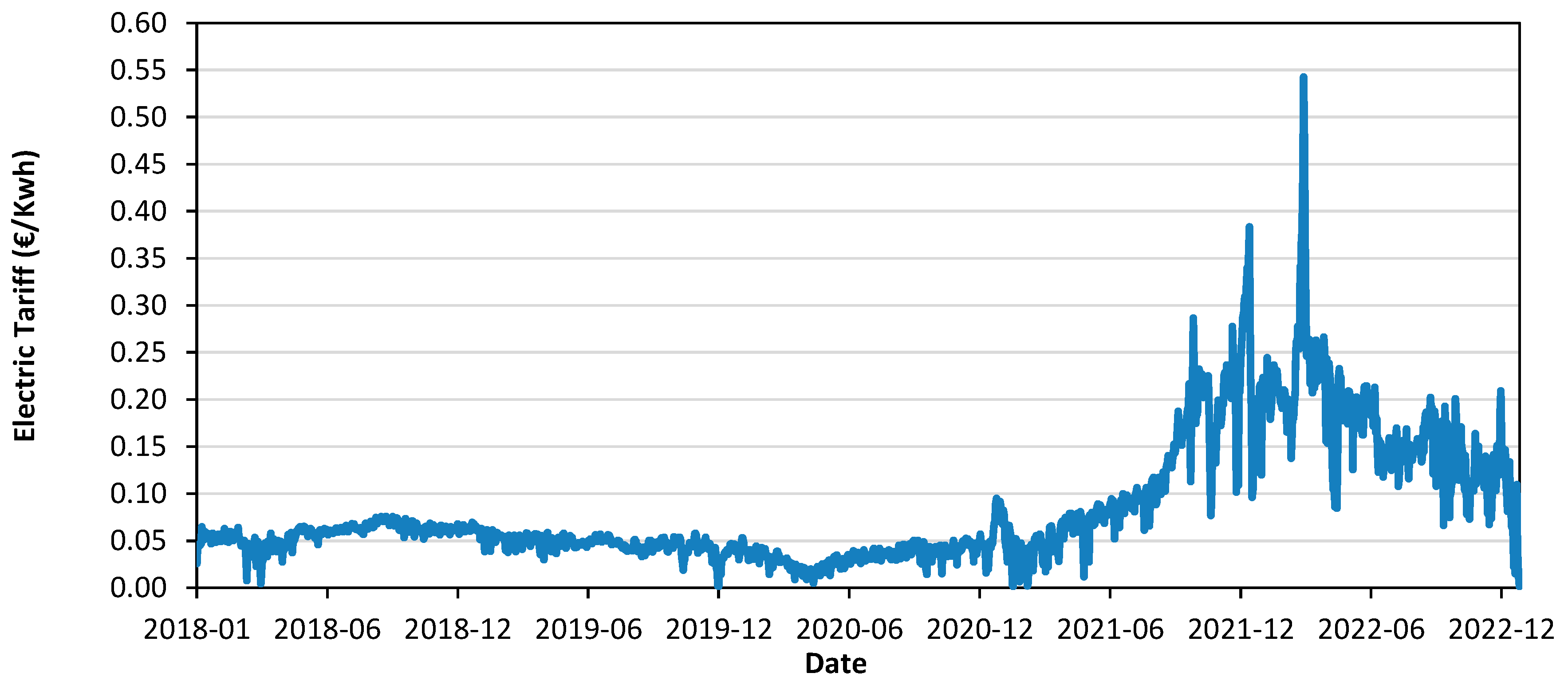
• The sensitivity analysis revealed important differences between the two design approaches regarding the electric tariff (TE), as can be observed in Table 13. The tolerance range of the electric tariff (TE) of the first approach had a defined width, whereas the tolerance range (TE) in the second approach was undefined because variation in this variable did not affect its ultimate solution.
• The solution obtained in the first approach was affected by significant variations in the electric tariff, as they were considered in the present work. In contrast, the solution obtained in the second approach remained unaffected by changes in the electric tariff, even when the electric tariff (TE) had extreme variations.
• Changes in the electric tariff primarily impacted operational costs, but they had a significant impact only on the ultimate solution of the first approach, which relied solely on LCC. The second approach, considering technical, economic, and environmental aspects, based on the AHP, resulted in a more robust solution that remained unchanged despite variations in the annual electricity tariff (TE).

In conclusion, the sensitivity analysis highlighted the importance of considering multiple variables and adopting a multi-criteria approach in PS design, incorporating technical, economic, and environmental factors. This approach leads to more robust solutions that are less sensitive to changes in variables such as interest rate (T_i), mean demand (Q_m), static head (ΔH), losses (R) in the setpoint curve, and electric tariff (TE). On the other hand, the first design approach, which relied solely on LCC, was more susceptible to variations in these variables.

References

1. Leiby, V.M.; Burke, M.E. Energy Efficiency Best Practices for North American Drinking Water Utilities; WRF: Albany, NY, USA, 2011. [Google Scholar]
2. Luna, T.; Ribau, J.; Figueiredo, D.; Alves, R. Improving energy efficiency in water supply systems with pump scheduling optimization. J. Clean. Prod. 2019, 213, 342–356. [Google Scholar] [CrossRef]
3. Makaremi, Y.; Haghighi, A.; Ghafouri, H.R. Optimization of Pump Scheduling Program in Water Supply Systems Using a Self-Adaptive NSGA-II; a Review of Theory to Real Application. Water Resour. Manag. 2017, 31, 1283–1304. [Google Scholar] [CrossRef]
4. Carpitella, S.; Brentan, B.; Montalvo, I.; Izquierdo, J.; Certa, A. Multi-criteria analysis applied to multi-objective optimal pump scheduling in water systems. Water Sci. Technol. Water Supply 2019, 19, 2338–2346. [Google Scholar] [CrossRef]
5. Martin-Candilejo, A.; Martin-Carrasco, F.J.; Santillán, D. How to select the number of active pumps during the operation of a pumping station: The convex hyperbola charts. Water 2021, 13, 1474. [Google Scholar] [CrossRef]
6. Wu, W.; Simpson, A.R.; Maier, H.R. Accounting for Greenhouse Gas Emissions in Multiobjective Genetic Algorithm Optimization of Water Distribution Systems. J. Water Resour. Plan. Manag. 2010, 136, 146–155. [Google Scholar] [CrossRef]
7. Torregrossa, D.; Capitanescu, F. Optimization models to save energy and enlarge the operational life of water pumping systems. J. Clean. Prod. 2019, 213, 89–98. [Google Scholar] [CrossRef]
8. Alandi, P.P.; Pérez, P.C.; Álvarez, J.F.O.; Hidalgo, M.M.; Martín-Benito, J.M.T. Pumping Selection and Regulation for Water-Distribution Networks. J. Irrig. Drain. Eng. 2005, 131, 273–281. [Google Scholar] [CrossRef]
9. Lamaddalena, N.; Khila, S. Efficiency-driven pumping station regulation in on-demand irrigation systems. Irrig. Sci. 2013, 31, 395–410. [Google Scholar] [CrossRef]
10. Karpenko, M.; Stosiak, M.; Šukevičius, Š.; Skačkauskas, P.; Urbanowicz, K.; Deptuła, A. Hydrodynamic Processes in Angular Fitting Connections of a Transport Machine’s Hydraulic Drive. Machines 2023, 11, 355. [Google Scholar] [CrossRef]
11. Olszewski, P. Genetic optimization and experimental verification of complex parallel pumping station with centrifugal pumps. Appl. Energy 2016, 178, 527–539. [Google Scholar] [CrossRef]
12. Cimorelli, L.; Covelli, C.; Molino, B.; Pianese, D. Optimal regulation of pumping station in water distribution networks using constant and variable speed pumps: A technical and economical comparison. Energies 2020, 13, 2530. [Google Scholar] [CrossRef]
13. Briceño-León, C.X.; Iglesias-Rey, P.L.; Martinez-Solano, F.J.; Mora-Melia, D.; Fuertes-Miquel, V.S. Use of fixed and variable speed pumps in water distribution networks with different control strategies. Water 2021, 13, 479. [Google Scholar] [CrossRef]
14. Deptuła, A.; Augustynowicz, A.; Stosiak, M.; Towarnicki, K.; Karpenko, M. The Concept of Using an Expert System and Multi-Valued Logic Trees to Assess the Energy Consumption of an Electric Car in Selected Driving Cycles. Energies 2022, 15, 4631. [Google Scholar] [CrossRef]
15. Saaty, T.L. Analytic Hierarchy Process; McGraw Hil: New York, NY, USA, 1980. [Google Scholar]
16. Saaty, T.L. Decision making with the analytic hierarchy process. Int. J. Serv. Sci. 2008, 1, 83–98. [Google Scholar] [CrossRef]
17. Aşchilean, I.; Badea, G.; Giurca, I.; Naghiu, G.S.; Iloaie, F.G. Choosing the optimal technology to rehabilitate the pipes in water distribution systems using the AHP method. Energy Procedia 2017, 112, 19–26. [Google Scholar] [CrossRef]
18. Kurbatova, A.; Abu-Qdais, H.A. Using multi-criteria decision analysis to select waste to energy technology for a mega city: The case of Moscow. Sustainability 2020, 12, 9828. [Google Scholar] [CrossRef]
19. Briceño-León, C.X.; Sanchez-Ferrer, D.S.; Iglesias-Rey, P.L.; Martinez-Solano, F.J.; Mora-Melia, D. Methodology for pumping station design based on analytic hierarchy process (AHP). Water 2021, 13, 2886. [Google Scholar] [CrossRef]
20. Briceño-León, C.X.; Iglesias-Rey, P.L.; Martínez-Solano, F.J.; Creaco, E. Integrating Demand Variability and Technical, Environmental, and Economic Criteria in Design of Pumping Stations Serving Closed Distribution Networks. J. Water Resour. Plan. Manag. 2023, 149, 04023002. [Google Scholar] [CrossRef]
21. Lee, C.; Tien, I. Sensitivity analysis of interdependency parameters using probabilistic system models. In Proceedings of the 13th International Conference on Applications of Statistics and Probability in Civil Engineering, Brussels, Belgium, 26–30 May 2019; pp. 1–13. [Google Scholar]
22. Morosini, A.F.; Haghshenas, S.S.; Haghshenas, S.S.; Choi, D.Y.; Geem, Z.W. Sensitivity analysis for performance evaluation of a real water distribution system by a pressure driven analysis approach and artificial intelligence method. Water 2021, 13, 1116. [Google Scholar] [CrossRef]
23. Jensen, H.; Jerez, D. A Stochastic Framework for Reliability and Sensitivity Analysis of Large Scale Water Distribution Networks. Reliab. Eng. Syst. Saf. 2018, 176, 80–92. [Google Scholar] [CrossRef]
24. Walski, T.; Creaco, E. Selection of pumping configuration for closed water distribution systems. J. Water Resour. Plan. Manag. 2016, 142, 04016009. [Google Scholar] [CrossRef]
25. Sanks, R.L. Pumping Station Design, 2nd ed.; Butterworth-Heinemann: Woburn, MA, USA, 1998. [Google Scholar]
26. Coelho, B.; Andrade-Campos, A.G. A new approach for the prediction of speed-adjusted pump efficiency curves. J. Hydraul. Res. 2016, 54, 586–593. [Google Scholar] [CrossRef]
27. Hydraulic Institute. Pump Life Cycle Costs: A Guide to LCC Analysis for Pumping Systems, 2nd ed.; Office of Energy Efficiency and Renewable Energy (EERE), Energy Efficiency Office, Advanced Manufacturing Office: Washington, DC, USA, 2001.
28. The European Union Comission. Commission Regulation (EU) N0 547/2012. Off. J. Eur. Union 2012, 4, 178–183. [Google Scholar]
29. Oficina Española del Cambio Climático (OECC). Factores de Emisión Registro de Huella de Carbono, Compensacion y Proyectos de Absorción de Dióxido de Carbono; Ministerio para la Transición Ecológica y el Reto Demográfico España: Madrid, Spain, 2022.
Figure 1. PS layout.
Water 15 03067 g001
Figure 2. Stages of the second PS approach.
Water 15 03067 g002
Figure 3. Variability of demand.
Water 15 03067 g003
Figure 4. Hourly pattern of electric tariff.
Water 15 03067 g004
Figure 5. Daily variability in electricity tariff.
Water 15 03067 g005