Regional Flow Influenced Recirculation Zones of Pump‒and‒Treat Systems for Groundwater Remediation with One or Two Injection Wells: An Analytical Comparison

Abstract

As a widely employed method for in situ remediation of groundwater contamination, the pump-and-treat (PAT) system involves the management of water recirculation between the extraction and injection wells. The recirculation zone (RZ) of an extraction-injection well pair in a confined aquifer has been well known. However, PAT systems are more frequently used in unconfined aquifers with a natural regional flow and may not only include one injection well. We develop comparable analytical models for an unconfined aquifer treated by two different system settings, including an extraction well and one injection well (1e/1i system) or two injection wells (1e/2i system). The role of regional groundwater flow is highlighted. Analytical solutions of RZs and recirculation ratios are obtained using complex potential functions, with a new treatment of the jump of the stream function at a branch cut. Results indicate that the shape of RZs and the recirculation ratio nonlinearly depend on several dimensionless parameters linked to the pumping rate and direction of regional flow. Compared to the 1e/1i system, the two injection wells in the 1e/2i system may reduce the integrity of RZs and decrease the recirculation ratio; however, they lead to a higher allowable pumping rate in satisfying the limitations of the water table in wells. This study suggests a useful methodology for analyzing PAT systems with multiple injection wells and provides new insights into RZs between extraction and injection wells.

1. Introduction

The pump-and-treat (PAT) method is widely used for in-situ remediation of groundwater contamination. Groundwater is pumped out from an extraction well in a PAT system and then treated to reduce pollutants [1,2,3]. In general, treated water is reinjected into aquifers through the original extraction borehole [4] or other wellbores specially prepared for injection [5,6,7,8,9]. Coordinated operation of the extraction and injection wells can accelerate groundwater remediation. It has been well known that a recirculation zone (RZ) may be developed between the extraction and injection wells, where groundwater is recharged by the injection well while being discharged towards the pumping well. Multiple RZs may exist at a site, including multiple injection wells, which may increase the difficulty of managing the recirculation. RZs also play important roles in projects of coastal groundwater management [10,11,12], Two-well tests [13,14], and thermal energy exploitation [15,16,17].

The regional groundwater flow significantly influences the RZ for the extraction/injection well pair [18,19]. To delineate the shape of RZs affected by the regional groundwater flow and estimate the fraction of flow rate in a RZ, both numerical modeling methods [20,21,22,23,24] and analytical solutions [25,26,27,28,29,30,31,32] have been applied. Numerical methods are powerful for complicated conditions, while the accuracy of results highly depends on the resolution of the model grid and the particle tracking process. In comparison, analytical solutions can reveal the exact and general impacts of the regional groundwater flow in typical conditions and can be used to provide simplified design tools for PAT systems.

The RZ of an extraction-injection well pair with a uniform regional flow has been analyzed in detail in the literature [11,18,28,33,34]. The conceptual model of the extraction-injection well pair in a PAT system is shown in Figure 1a, where the system includes one extraction well and one injection well (marked as the 1e/1i system in this study). Existing analytical solutions of the flow were typically derived for a 1e/1i system in a confined aquifer [28], but they can be extended to determine the RZ shape in an unconfined aquifer, as shown in Figure 1a. A poorly known effect is the limitation of water table heights in the injection and extraction wells (to be neither too high nor too low), which may lead to a threshold of the recirculation ratio and influence the efficiency of the PAT system.

Multiple injection wells can be used in a PAT system, but they may lead to more complicated patterns of RZs that are not well known. A typical example is the 1e/2i system shown in Figure 1b, where an extraction well gains water from double injection wells. Christ et al. (1999) [25] developed analytical solutions for flow zones for multiple extraction-injection well pairs in a confined aquifer, i.e., for the ne/ni system, where n extraction wells are linked with n injection wells. Unfortunately, the solutions are not available for the 1e/2i system. Shi et al. (2020) [12] analyzed RZs of the 1e/ni system in a coastal confined aquifer, where the injection wells are located in the downgradient area of the regional flow with respect to the extraction well. However, for the regional groundwater flow with an arbitrary direction, the exact RZ patterns of the 1e/ni system are still poorly known. We expect that analyzing the 1e/2i system is a reasonable step for investigating the general behaviors of the 1e/ni system.

In this study, we delineate the RZs of the 1e/2i system in detail and estimate the recirculation ratio using the analytical method. Results are compared with the RZ and recirculation ratio of the 1e/1i system. Conceptual models and complex potential functions of groundwater flow driven by the 1e/1i and 1e/2i systems are presented in Section 2 for an unconfined aquifer with a uniform regional flow. Then, analytical solutions are presented in Section 3 and Section 4, respectively, for the RZ in the 1e/1i system and the RZs in the 1e/2i system. The recirculation ratio and the performance of the two kinds of PAT systems are compared in Section 5. The study results provide new insights into the design of a PAT system influenced by regional groundwater flow.

2. Conceptual Model and Complex Potential Functions

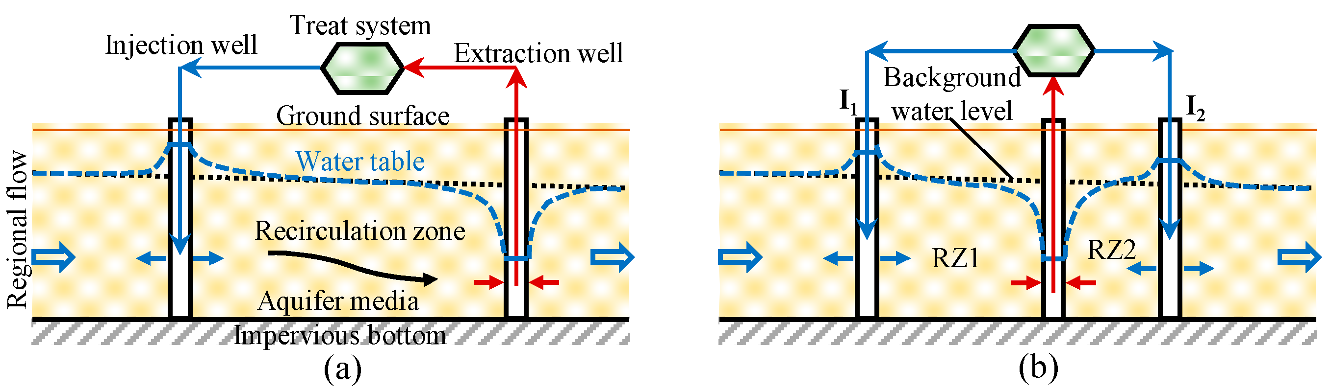
2.1. Simplified Conceptual Model

The conceptual model of groundwater flow for the 1e/1i and 1e/2i systems is shown in Figure 1, which includes simplifications in hydrogeological conditions: (1) The aquifer is a horizontally extending unconfined aquifer, composed of homogeneous and isotropic media with a flat impervious bottom, while does not influenced by the vertical infiltration recharge or discharge; (2) The regional groundwater flow in the aquifer is uniform in an area that is significantly larger than the well-influenced zone at the site; (3) At the site of the PAT system, groundwater flow is controlled by an extraction well and one injection well (1e/1i system) or two injection wells (1e/2i system); (4) All wells are fully penetrated into the aquifer, and the total injection flow rate is equal to the extraction flow rate; (5) The regional groundwater flow and local flow driven by wells are both in a steady state. Based on these simplifications, we adopt the Dupuit-Forchheimer assumption [35] to investigate the flow in a plan view, i.e., neglecting the vertical flow velocity.

Using the Cartesian coordinate system, as (X, Y) shown in Figure 2, the regional groundwater flow can be quantified as:

$$q_0\cos \alpha =-K{h}_0\frac{\partial h_0}{\partial X}, q_0\sin \alpha =-K{h}_0\frac{\partial h_0}{\partial Y}$$

(1)

where: q₀ is the constant flow rate per unit width of the aquifer [L²T⁻¹], α is the counterclockwise angle of the flow direction with respect to the X axis [0, π]; h₀ is the background water level in the aquifer related to the bottom [L], and K is the hydraulic conductivity of the aquifer media [LT⁻¹]. The water table height is a function of the position, h(X, Y), and becomes different from the background water level, h₀(X, Y), due to the impacts of the extraction and injection wells. For the 1e/1i system (Figure 2a), the extraction well (E) and the injection well (I) are allocated at (d, 0) and (−d, 0), respectively, with a distance of 2d [L] between them. The flow rates of the extraction and injection wells are +Q and −Q [L³T⁻¹], respectively, where Q is a constant positive value. For the 1e/2i system (Figure 2b), the extraction well (E) is allocated at (0, 2d), whereas the double injection wells, I₁ and I₂, are allocated at (0, b) and (0, −b), respectively. The flow rates of the injection wells are the same as −Q/2, where Q is the pumping rate of the extraction well. Local groundwater discharges along the directions of the X and Y coordinates, q_X and q_Y [L²T⁻¹], respectively, can be estimated as:

$$q_X=h{V}_X=-Kh\frac{\partial h}{\partial X}, q_Y=h{V}_Y=-Kh\frac{\partial h}{\partial Y}$$

(2)

where: V_X [LT⁻¹] and V_Y [LT⁻¹] are the Darcy velocities in the X-direction and Y-direction, respectively.

2.2. Complex Potential Function

The 2D steady-state flow field for an infinite aquifer with a uniform regional flow and multiple wells can be expressed by a complex function [35,36],

$$\Omega =\Phi +i\Psi ={\Phi }_0-q_{0}Z{e}^{-\mathrm{i}\alpha }+\frac{1}{2\pi }{\displaystyle \sum _{j=1}^N{Q}_j}\ln \left(Z-Z_j\right)$$

(3)

where: Ω is the complex potential; Φ and Ψ are the discharge potential and stream function [L³T⁻¹], respectively; Φ₀ is a reference value of the discharge potential depending on the background water level; Q_j is the flow rate [L³T⁻¹] of the j-th well (Q_j > 0 for an extraction well, Q_j < 0 for an injection well); N is the number of wells; the complex variable, Z = X + iY, defines the position at (X, Y), while Z_j = X_j + iY_j denotes the position of the j-th well. For the unconfined aquifer in this study, the discharge potential and stream function can be defined as [35]:

$$\Phi =\frac{1}{2}K{h}^2, \frac{\partial \Psi }{\partial X}=q_y, \frac{\partial \Psi }{\partial Y}=-q_x$$

(4)

Generic solutions of the discharge potential and stream function according to Equation (3) have been obtained as follows [36]:

$$\Phi ={\Phi }_0-q_0\left(X\cos \alpha +Y\sin \alpha \right)+{\displaystyle \sum _{j=1}^N\frac{Q_j}{4\pi }}\ln \left[{(X-X_j)}^2+{(Y-Y_j)}^2\right]$$

(5)

$$\Psi =q_0\left(X\sin \alpha -Y\cos \alpha \right)+{\displaystyle \sum _{j=1}^N\frac{Q_j}{2\pi }}\arg (Z-Z_j)$$

(6)

where: arg(Z − Z_j) is the argument of Z − Z_j, which is multi-valued. When using MATLAB for computation, the argument is usually calculated with atan2(Y − Y_j, X − X_j) that takes values in the range of (−π, π]. Substituting the well locations of the 1e/1i system (Figure 2a) into Equations (5) and (6), we have

$$\Phi =\frac{1}{2}K{h}_{\mathrm{ref}}^2-q_0\left(X\cos \alpha +Y\sin \alpha \right)+\frac{Q}{4\pi }\ln \frac{{\left(X-d\right)}^2+Y^2}{{\left(X+d\right)}^2+Y^2}$$

(7)

$$\Psi =q_0\left(X\sin \alpha -Y\cos \alpha \right)+\frac{Q}{2\pi }[\mathrm{atan}2(Y,X-d)-\mathrm{atan}2(Y,X+d)]$$

(8)

where: Q is the flow rate of the extraction well; h_ref is the background water level at X = 0 and Y = 0. For the 1e/2i system (Figure 2b), the solutions become:

$$\Phi =\frac{1}{2}K{h}_{\mathrm{ref}}^2-q_0\left(X\cos \alpha +Y\sin \alpha \right)+\frac{Q}{4\pi }\ln \frac{{\left(X-2d\right)}^2+Y^2}{\sqrt{\left[X^2+{(Y-b)}^2\right]\left[X^2+{(Y+b)}^2\right]}}$$

(9)

$$\Psi =q_0\left(X\sin \alpha -Y\cos \alpha \right)+\frac{Q}{2\pi }[\mathrm{atan}2(Y,X-2d)-\frac{\mathrm{atan}2(Y+b,X)+\mathrm{atan}2(Y-b,X)}{2}]$$

(10)

Note that atan2(Y, X) in MATLAB is a special representation of the multivalued argument function as arctan(Y/X).

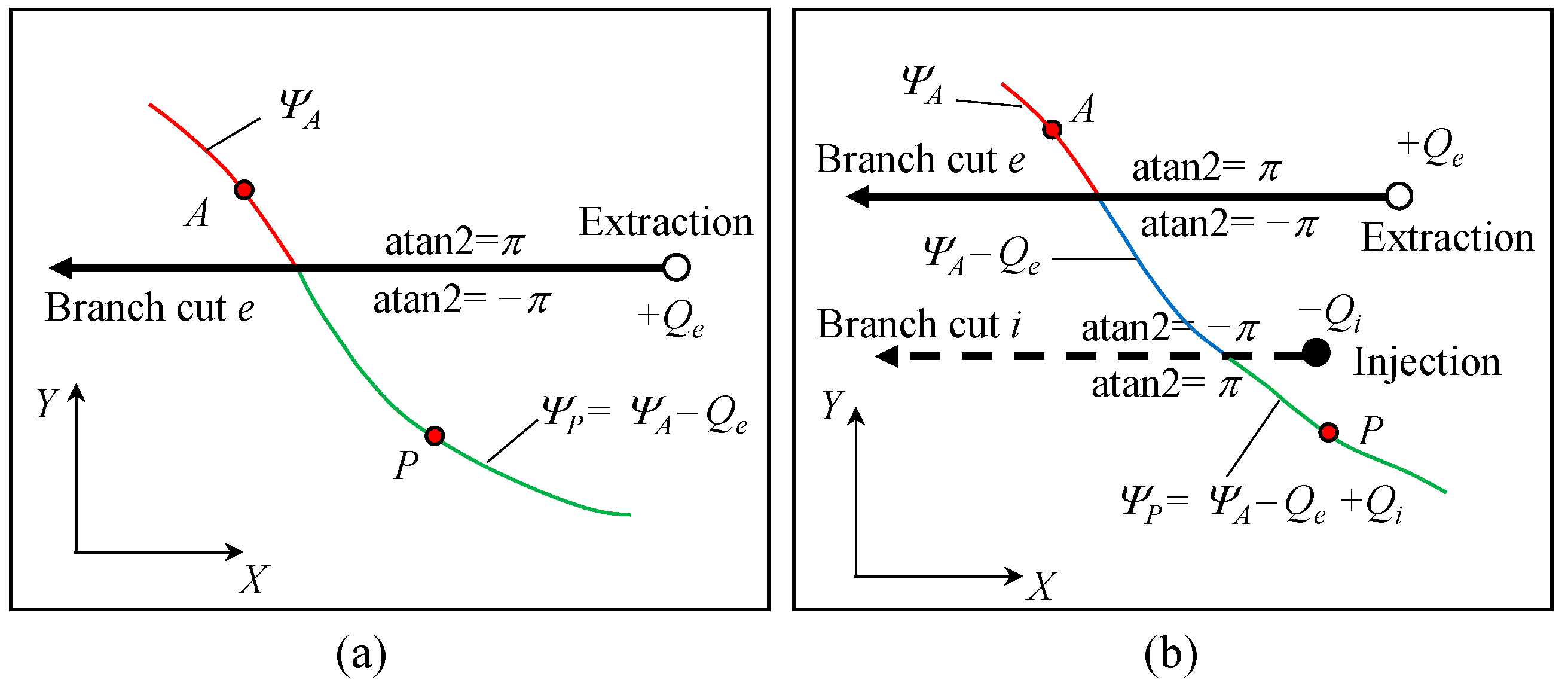
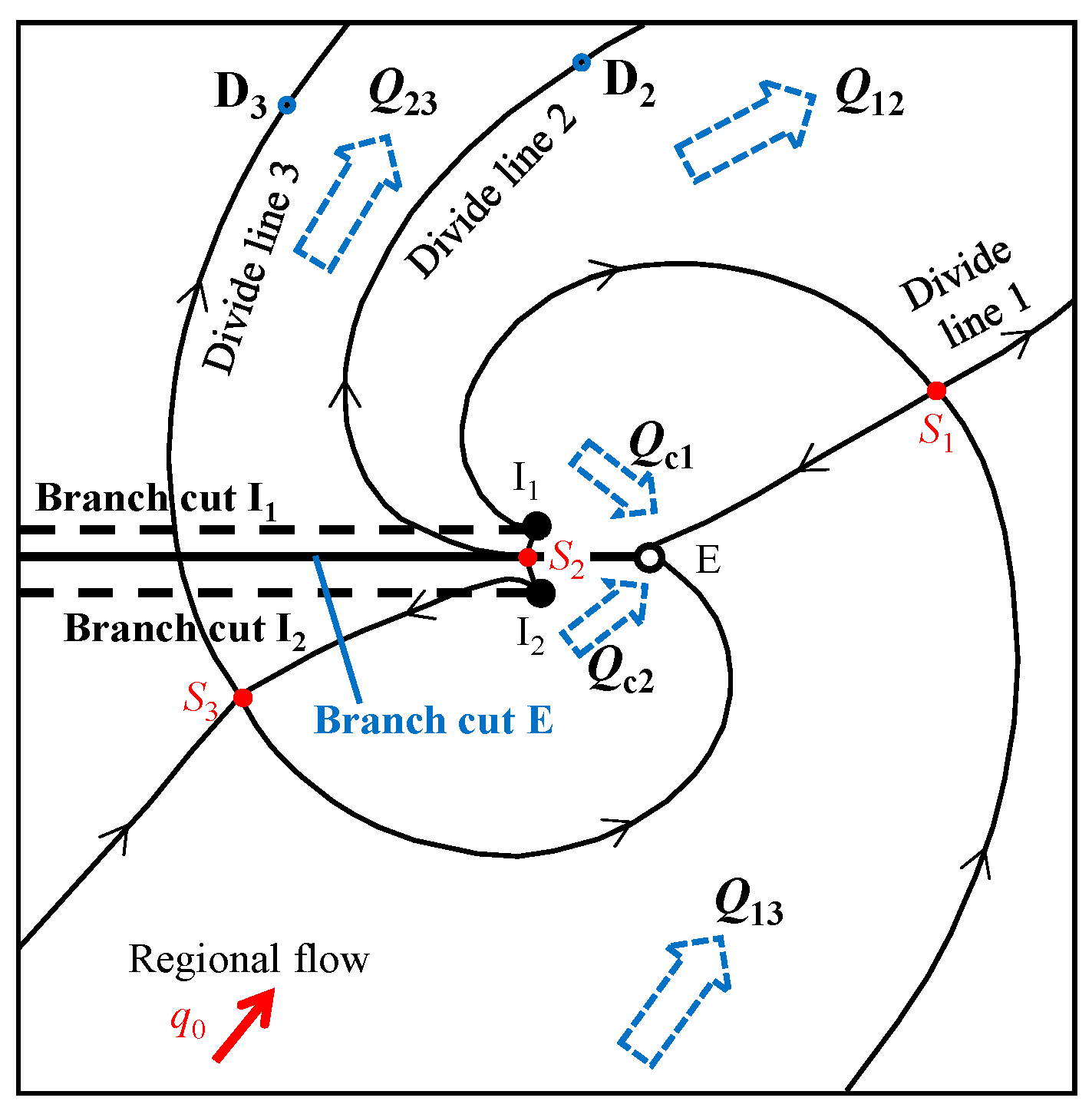
2.3. Streamline and Branch Cuts

The contours of the stream function can be applied to represent streamlines for the 2D steady-state groundwater flow. However, a challenge for delineating a streamline using the stream function is the branch cut [37,38,39,40] arising from the argument function. As shown in Figure 3, a branch cut is a line that extends from the well toward the negative direction of the X axis. The relative argument of points on a cut line is either π or −π as estimated with the atan2(Y − Y_j, X − X_j) function in MATLAB. When a streamline links points A and P on the sides of the branch cut extending from an extraction well (Figure 3a), the following relationship should be considered:

$${\Psi }_P={\Psi }_A+\frac{Q_e}{2\pi }(-\pi -\pi )={\Psi }_A-Q_e$$

(11)

where: Q_e is the extraction flow rate; Ψ_A and Ψ_P are the stream function values of A and P, respectively. When a part of the streamline between A and P extends across branch cut lines of several wells (an example is shown in Figure 3b), the relationship of stream function values can be accounted for by

$${\Psi }_P={\Psi }_A-{\displaystyle \sum _{i=1}^M{Q}_i}$$

(12)

where: M is the number of branch cut lines between A and P (Figure 3b); Q_i is the well flow rate of the i-th branch cut. As a result, when the branch cut lines in Figure 3b are generated from the three wells of the 1e/2i system (Figure 2b), there must be Ψ_P = Ψ_A.

3. Analytical Solutions of 1e1i System

3.1. Dimensionless Functions

We introduce the following dimensionless variables for the 1e/1i system,

$$x=\frac{X}{d}, y=\frac{Y}{d}, \varphi =\frac{2\pi \Phi }{Q}, {\varphi }_{\mathrm{ref}}=\frac{\pi K}{Q}{h}_{\mathrm{ref}}^2, \psi =\frac{2\pi \Psi }{Q}, q_D=\frac{2\pi d{q}_0}{Q}$$

(13)

According to Equations (7) and (8), the dimensionless discharge potential and stream functions can be expressed as:

$$\varphi (x,y)={\varphi }_{\mathrm{ref}}-q_D\left(x\cos \alpha +y\sin \alpha \right)+\frac{1}{2}\ln \frac{{\left(x-1\right)}^2+y^2}{{\left(x+1\right)}^2+y^2}$$

(14)

$$\psi (x,y)=q_D\left(x\sin \alpha -y\cos \alpha \right)+\mathrm{atan}2\left(y,x-1\right)-\mathrm{atan}2\left(y,x+1\right)$$

(15)

3.2. Stagnation Points

In general, there are two stagnation points in the flow field of the 1e/1i system, denotds S₁ and S₂ (Figure 4). They may fall on the X axis (Figure 4a) or Y axis (Figure 4b) or at other places. The Darcy velocities at a stagnation point satisfy V_X = 0 and V_Y = 0, as well as dΩ/dz = 0. It leads to an equation expressed in a dimensionless manner as follows:

$$z^2-\left(1+\frac{2e^{i\alpha }}{q_D}\right)=0$$

(16)

where: z = x + iy. The roots of Equation (16) yield the positions of S₁ at z₁ = x₁ + iy₁, and S₂ at z₂ = x₂ + iy₂. We obtain:

$$x_1=\sqrt{{\left(\frac{1}{4}+\frac{1}{q_D^2}+\frac{\cos \alpha }{q_D}\right)}^{1/2}+\left(\frac{1}{2}+\frac{\cos \alpha }{q_D}\right)}, y_1=\sqrt{{\left(\frac{1}{4}+\frac{1}{q_D^2}+\frac{\cos \alpha }{q_D}\right)}^{1/2}-\left(\frac{1}{2}+\frac{\cos \alpha }{q_D}\right)}$$

(17)

$$x_2=-x_1, y_2=-y_1$$

(18)

Note that the stagnation point S₁ falls on the right-side zone of the Y axis, or just on the Y axis, while S₂ falls on the opposite zone, or also just on the Y axis.

Figure 4. Typical patterns of flow zones for the 1e/1i system: (a) a complete RZ when α = 0; (b) an approximate prismatic RZ when α = π; (c) a rotational symmetrical RZ when α = π/4; (d) absence of the RZ when α = π/4. I−IV are the number of flow zones. Zone-I is the regional flow captured by the extraction well E and filled with red; zone-II is the regional flow contributed by the injection well I and filled with blue; zone-III is the RZ and filled with green; zone-IV is filled with white. Arrows indicate groundwater flow direction on the streamlines.

Figure 4. Typical patterns of flow zones for the 1e/1i system: (a) a complete RZ when α = 0; (b) an approximate prismatic RZ when α = π; (c) a rotational symmetrical RZ when α = π/4; (d) absence of the RZ when α = π/4. I−IV are the number of flow zones. Zone-I is the regional flow captured by the extraction well E and filled with red; zone-II is the regional flow contributed by the injection well I and filled with blue; zone-III is the RZ and filled with green; zone-IV is filled with white. Arrows indicate groundwater flow direction on the streamlines.

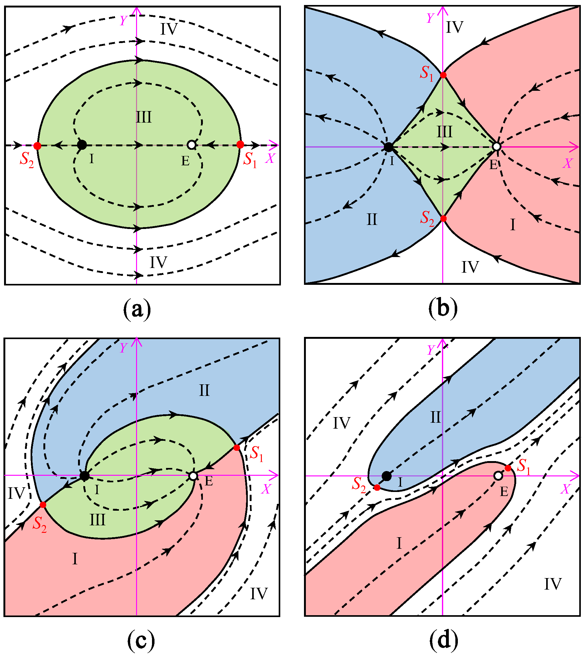
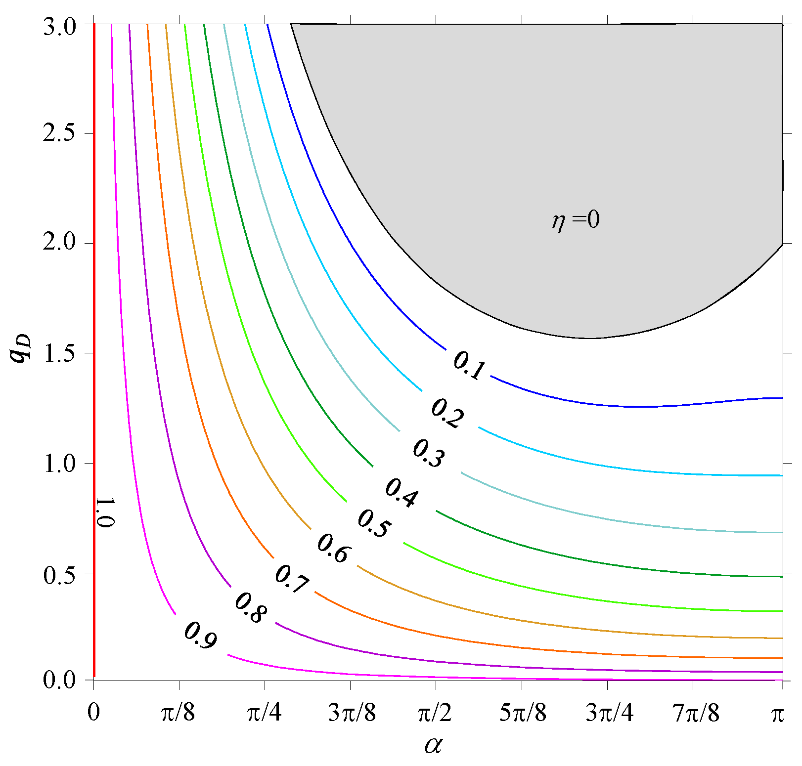
3.3. Recirculation Zone

Partitioning flow zones of the 1e/1i system can be performed by delineating streamlines between the two stagnation points, S₁ and S₂. Four streamlines are linked by a stagnation point, which serves as a divide between flow zones. In general, four flow zones are partitioned by these divide lines, as shown in Figure 4: Zone-I includes groundwater captured by the extraction well from the regional flow; zone-II includes water released from the injection well and joints to the regional flow; zone-III is the RZ; and zone-IV includes groundwater that is not exchanged with wells. We denote stream function values at S₁ and S₂ as ψ(x₁, y₁) and ψ(x₂, y₂), respectively. Substituting Equations (17) and (18) into Equation (15), we have

$$\psi \left(x_1,y_1\right)=-\psi \left(x_2,y_2\right)$$

(19)

When the RZ (zone-III) exists, the discharge (Q_c) of the regional flow captured by the extraction well can be estimated from the absolute difference between the stream function values of S₁ and S₂, leading to:

$$\begin{gathered} Q_c=\frac{Q}{2\pi }\left|\psi \left(x_1,y_1\right)-\psi \left(x_2,y_2\right)\right| \\ =\frac{1}{\pi }\left|q_D\left(x_1\sin \alpha -y_1\cos \alpha \right)+\mathrm{atan}2\left(y_1,x_1-1\right)-\mathrm{atan}2\left(y_1,x_1+1\right)\right| \end{gathered}$$

(20)

Note that Q − Q_c yields the flow rate of water in the RZ. Thus, the recirculation ratio, η = (Q − Q_c)/Q, can be calculated as:

$$\eta =1-\frac{Q_c}{Q}=1-\frac{1}{\pi }\left|q_D\left(x_1\sin \alpha -y_1\cos \alpha \right)+\mathrm{atan}2\left(y_1,x_1-1\right)-\mathrm{atan}2\left(y_1,x_1+1\right)\right|$$

(21)

Equation (21) is the analytical solution of the recirculation ratio for the 1e/1i system.

The RZ of the 1e/1i system is controlled by two dimensionless parameters: q_D and α. When α = 0, both stagnation points fall on the X axis, forming a complete RZ (Figure 4a), where the injected water totally returns to the extraction well, i.e., η = 1. When α = π, stagnation points fall on the Y axis and form a RZ that is symmetric about the X and Y axes (Figure 4b), where a part or all of the injected water returns to the extraction well, i.e., η ≤ 1. When 0 < α < π, the RZ may have a shape of rotational symmetry about the origin of coordinates (Figure 4c) with a recirculation ratio that is smaller than 1, i.e., η < 1. It is also possible that the RZ does not exist when q_D is significantly large (Figure 4d), leading to η ≤ 0 as estimated by substituting the q_D value into Equation (21). In this situation, the exact recirculation ratio should be η = 0. Figure 5 shows the dependency of η on q_D and α. It is clear that when both the angle and relative rate of the regional flow are high (α > π/2, q_D > 2), the RZ does not exist and the recirculation ratio is zero.

The recirculation ratio is also bounded by the limitation of water table height in the unconfined aquifer. The water table height, h(x, y), should not be very high (to avoid being close to the ground surface) or very low (to avoid being close to the aquifer bottom) within the wells. It implies that the discharge potential at the PAT site has a limited range, which can be expressed as

$${\Phi }_{\min }\le \Phi \le {\Phi }_{\max }$$

(22)

where: Φ_min and Φ_max are, respectively, the allowable minimum and maximum values of the discharge potential. The water level within the extraction well yields the lowest discharge potential at the site, Φ_ext, which can be estimated with Equation (7) by using X = d and Y = r_e, where r_e is the radius of the extraction well. It leads to

$${\Phi }_{\mathrm{ext}}=\frac{1}{2}K{h}_{\mathrm{ref}}^2-q_0\left(d\cos \alpha +r_e\sin \alpha \right)+\frac{Q}{4\pi }\ln \frac{r_e^2}{4d^2+r_e^2}$$

(23)

The limitation of this lowest discharge potential, is Φ_ext > Φ_min, which leads to

$$q_D\ge q_{\mathrm{ext}}, q_{\mathrm{ext}}=\frac{q_{0}d\ln [1+(4d^2/r_e^2)]}{K{h}_{\mathrm{ref}}^2-2q_0\left(d\cos \alpha +r_e\sin \alpha \right)-2{\Phi }_{\min }}$$

(24)

The water level within the injection well yields the highest discharge potential at the site, Φ_inj, which can be estimated with Equation (7) by using X = −d and Y = −r_i, where r_i is the radius of the injection well. It leads to

$${\Phi }_{\mathrm{inj}}=\frac{1}{2}K{h}_{\mathrm{ref}}^2+q_0\left(d\cos \alpha +r_i\sin \alpha \right)+\frac{Q}{4\pi }\ln \frac{4d^2+r_i^2}{r_i^2}$$

(25)

The limitation of this highest discharge potential, is Φ_inj ≤ Φ_max, which then leads to

$$q_D\ge q_{\min }, q_{\mathrm{inj}}=\frac{d{q}_0\ln [1+(4d^2/r_e^2)]}{2{\Phi }_{\max }-K{h}_{\mathrm{ref}}^2-2q_0\left(d\cos \alpha +r_i\sin \alpha \right)}$$

(26)

An integrated consideration of both Equations (24) and (26) yields

$$q_D\ge q_{\min }, q_{\min }=\max \{q_{\mathrm{ext}},q_{\mathrm{inj}}\}$$

(27)

By replacing q_D by q_min in Equation (21), a critical value of the recirculation ratio, η_c, can be obtained as

$${\eta }_c=1-\frac{1}{\pi }\left|q_{\min }\left(x_1\sin \alpha -y_1\cos \alpha \right)+\mathrm{atan}2\left(y_1,x_1-1\right)-\mathrm{atan}2\left(y_1,x_1+1\right)\right|$$

(28)

As a result, the real recirculation ratio should be lower than η_c, because the η value generally decreases with the increasing q_D value (Figure 5).

4. Analytical Solutions of 1e2i System

4.1. Dimensionless Functions, Stagnation Points and Divide Lines

For the 1e/2i system, an additional parameter beside the parameters defined in Equation (13) is introduced, as follows:

$$B=\frac{b}{d}$$

(29)

Then, the dimensionless functions of the discharge potential (ϕ) and the stream function (ψ) can be expressed as:

$$\varphi ={\varphi }_{\mathrm{ref}}-q_D\left(x\cos \alpha +y\sin \alpha \right)+\frac{1}{2}\ln \frac{{\left(x-2\right)}^2+y^2}{\sqrt{\left[x^2+{(y-B)}^2\right]\left[x^2+{(y+B)}^2\right]}}$$

(30)

$$\psi =q_D\left(x\sin \alpha -y\cos \alpha \right)+\mathrm{atan}2\left(y,x-2\right)-\frac{1}{2}\left[\mathrm{atan}2(y-B,x)+\mathrm{atan}2(y+B,x)\right]$$

(31)

The stagnation points are linked with the equation dΩ/dz = 0, where z represents the dimensionless complex, z = x + iy, and then the equation can be written as:

$$z^3-2z^2+\left(B^2-\frac{2}{q_D{e}^{-i\alpha }}\right)z-\left(2B^2+\frac{B^2}{q_D{e}^{-i\alpha }}\right)=0$$

(32)

For the 1e/2i system, typical patterns of the stagnation points and divide lines are shown in Figure 6. Three stagnation points are distributed around wells, denoted as S₁ at (x₁, y₁), S₂ at (x₂, y₂), and S₃ at (x₃, y₃), where divide lines linking S₁ and S₃ partition the regional groundwater flow into three parts, among which the middle part is captured by the extraction well. Two RZs exist among the extraction well and injection wells; one gains water from I₁ and another gains water from I₂. These two RZs are demarcated by a division line between points S₂ and E. The discharge rate of the regional flow captured by the extraction well, Q₁₃, can be estimated from the absolute difference between the stream function values of S₁ and S₃, leading to:

$$Q_{13}=\frac{Q}{2\pi }\left|\psi \left(S_1\right)-\psi \left(S_3\right)\right| \mathrm{or} Q_{13}=\frac{Q}{2\pi }\left|\psi \left(x_1,y_1\right)-\psi \left(x_3,y_3\right)\right|$$

(33)

The discharge rate of downgradient flow between S₁ and S₂ can be estimated from the absolute difference between the stream function values of S₁ and D₂, where D₂ is a point on the downgradient streamline linking S₂ over a long distance (Figure 6). Thus,

$$Q_{12}=\frac{Q}{2\pi }\left|\psi \left(S_1\right)-\psi \left(D_2\right)\right|$$

(34)

The relationship between ψ(D₂) and ψ(S₂) depends on jumps of the steam function caused by branch cut lines between D₂ and S₂, as follows:

$$\psi \left(D_2\right)=\psi \left(S_2\right)-\pi , \mathrm{when} y_2 > 0; \psi \left(D_2\right)=\psi \left(S_2\right)+\pi , \mathrm{when}{y}_2<0$$

(35)

A similar analysis can be performed for the discharge rate of downgradient flow between S₂ and S₃, which leads to:

$$Q_{23}=\frac{Q}{2\pi }\left|\psi \left(D_3\right)-\psi \left(D_2\right)\right|=\frac{Q}{2\pi }\left|\psi \left(S_3\right)-\psi \left(D_2\right)\right|$$

(36)

where: D₃ is a point on the downgradient streamline linking S₃ with a long distance (Figure 6). The value of ψ(D₃) is equal to ψ(S₃), because the streamline between S₃ and D₃ is influenced by three branch cut lines.

The Q₁₂, Q₁₃, and Q₂₃ values satisfy the following equation:

$$Q_{13}=Q_{12}+Q_{23}$$

(37)

Note that the discharge rate Q₁₂ is a part of the injected flow from I₁, and then the recirculation flow rate from I₁ to E can be estimated as

$$Q_{c1}=\frac{1}{2}Q-Q_{12}$$

(38)

Further, the recirculation flow rate from I₂ to E can be estimated as

$$Q_{c2}=\frac{1}{2}Q-Q_{23}$$

(39)

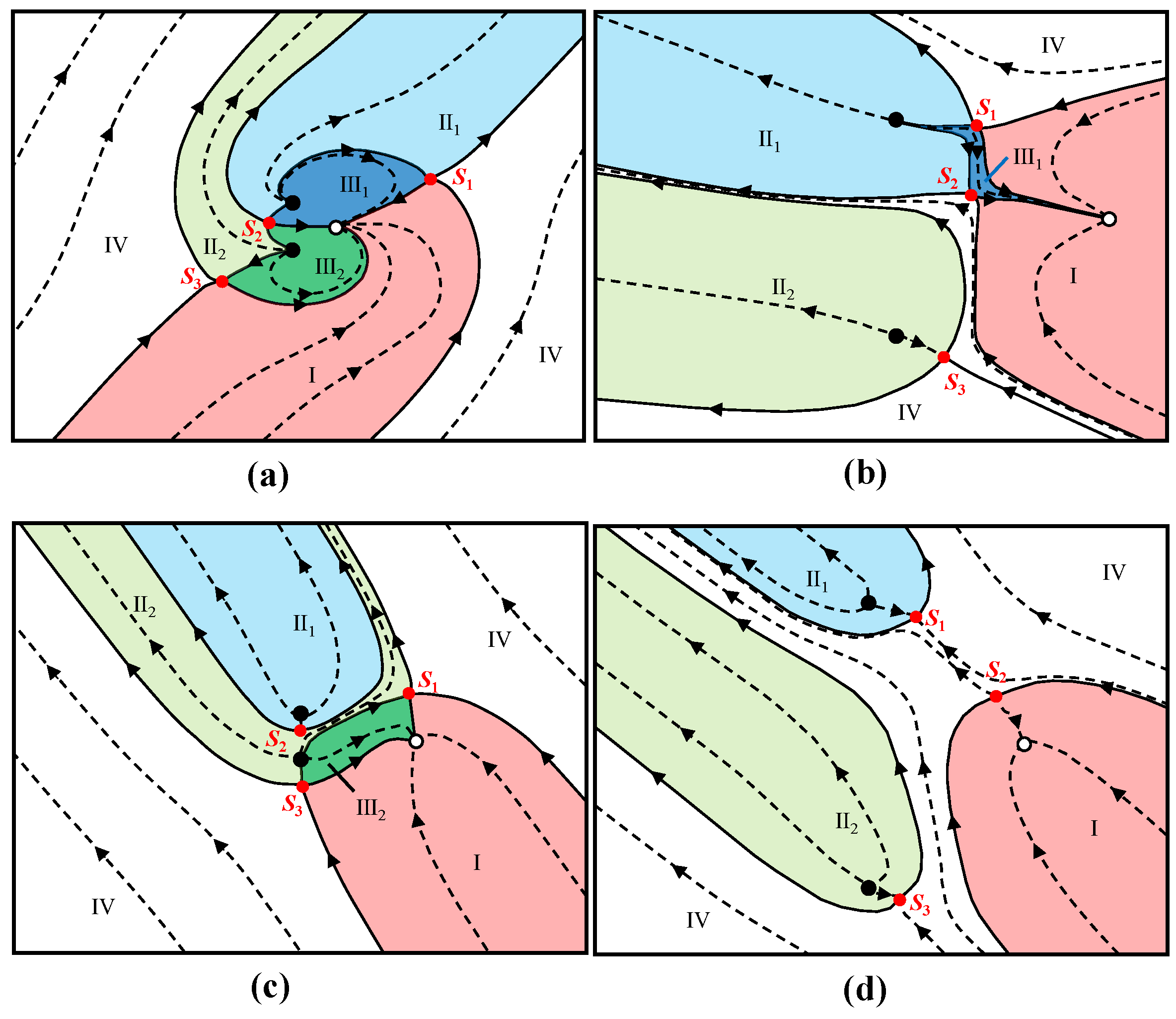
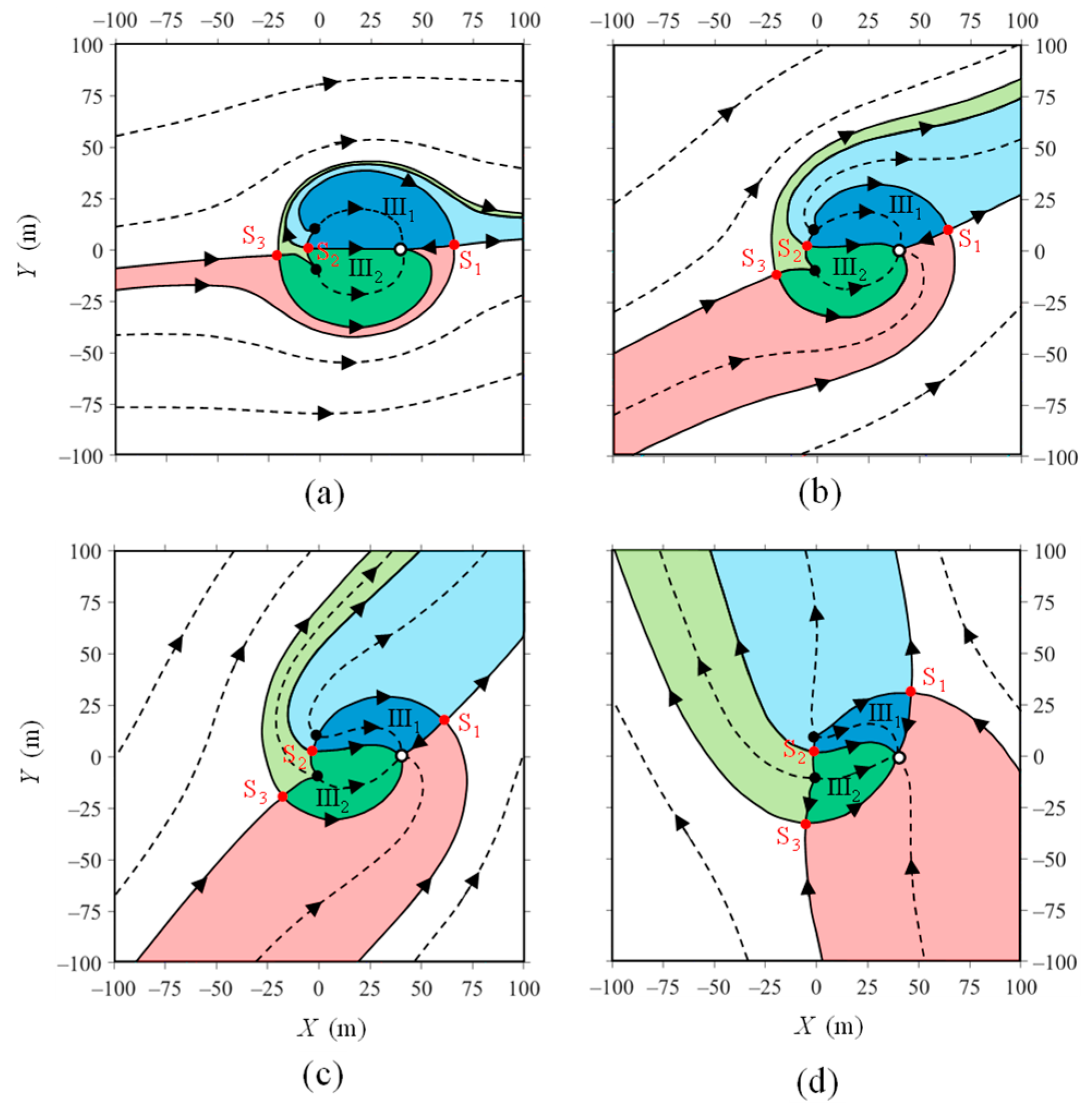
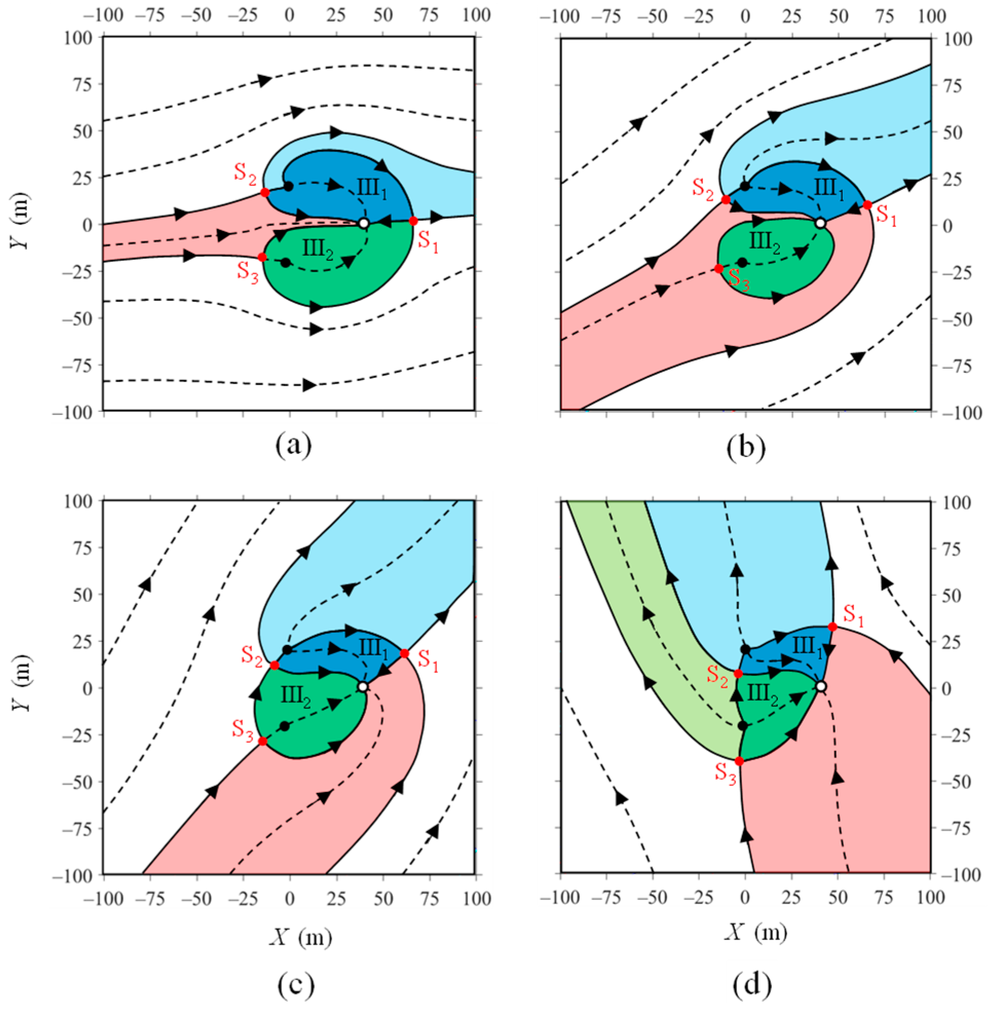
4.2. Patterns of Flow Zones

More flow zones can be partitioned in the 1e/2i system than zones in the 1e/1i system, as shown in Figure 7. In general, outside divide lines are identified to delineate zone IV of the regional groundwater flow that is not directly connected to wells and links stagnation points S₁ and S₃. The stagnation S₂ falls in the area bounded by these division lines and controls the patterns of RZs. The patterns of flow zones can be basically classified into four types:

(1)

Both RZs of the injection wells I₁ and I₂ are developed, as shown in zones III₁ and III₂ in Figure 7a. The extraction well gains water from zones I (regional flow) and RZs. The injection wells I₁ and I₂ also contribute water to zones II₁ and II₂, respectively, for the downgradient regional flow. The discharge rates, Q₁₂, Q₁₃, and Q₂₃, satisfy the following relationship:

$$Q_{12}<Q/2, Q_{23}<Q/2, Q_{13}<Q$$

(40)

In this situation, the recirculation ratio can be estimated as:

$${\eta }_1=\frac{1}{2}-\frac{Q_{12}}{Q}, {\eta }_2=\frac{1}{2}-\frac{Q_{23}}{Q}, \eta ={\eta }_1+{\eta }_2$$

(41)

(2)

Only the RZ of injection well I₁ exists, as zone III₁ in Figure 7b. The flow contributed from the injection well, I₂, totally joins the downgradient regional flow behind S₃. The discharge rates, Q₁₂, Q₁₃, and Q₂₃, satisfy the following relationship:

$$Q_{12}<Q/2, Q_{23}>Q/2, Q_{13}<Q$$

(42)

In this situation, the recirculation ratio can be estimated as:

$${\eta }_1=\frac{1}{2}-\frac{Q_{12}}{Q}, {\eta }_2=0, \eta ={\eta }_1$$

(43)

(3)

Only the RZ of the injection well I₂ exists, as zone III₂ in Figure 7c. The flow contributed from this injection well totally joins the downgradient regional flow behind S₂. The discharge rates, Q₁₂, Q₁₃, and Q₂₃, satisfy the following relationship:

$$Q_{12}>Q/2, Q_{23}<Q/2, Q_{13}<Q$$

(44)

In this situation, the recirculation ratio can be estimated as:

$${\eta }_1=0, {\eta }_2=1-\frac{Q_{13}}{Q}, \eta ={\eta }_2$$

(45)

(4)

Both RZs of the injection wells I₁ and I₂ do not exist, as shown in Figure 7d. Water contributed from the injection wells totally joins the downgradient regional flow. The discharge rates, Q₁₂, Q₁₃, and Q₂₃, satisfy the following relationship:

$$Q_{12}>Q/2, Q_{23}>Q/2, Q_{13}>Q$$

(46)

In this situation, the recirculation ratio is zero, with η = η₁ = η₂ = 0.

Figure 7. Flow zones of the 1e/2i system in different situations: (a) including two RZs denoted as zones III₁ and III₂; (b) including a RZ of III₁; (c) including a RZ of III₂; (d) absence of RZs. I−IV are the number of flow zones. Zone I is the regional flow captured by the extraction well E and filled with red; zone II₁ is the regional flow contributed by the injection well I₁ and filled with light blue; zone II₂ is the regional flow contributed by the injection well I₂ and filled with light green; zones III₁ and III₂ are RZ of the injection well I₁ and RZ of the injection well I₂, respectively, and filled with dark blue and dark green; zone IV is the regional groundwater flow and filled with white. Arrows indicate groundwater flow direction.

Figure 7. Flow zones of the 1e/2i system in different situations: (a) including two RZs denoted as zones III₁ and III₂; (b) including a RZ of III₁; (c) including a RZ of III₂; (d) absence of RZs. I−IV are the number of flow zones. Zone I is the regional flow captured by the extraction well E and filled with red; zone II₁ is the regional flow contributed by the injection well I₁ and filled with light blue; zone II₂ is the regional flow contributed by the injection well I₂ and filled with light green; zones III₁ and III₂ are RZ of the injection well I₁ and RZ of the injection well I₂, respectively, and filled with dark blue and dark green; zone IV is the regional groundwater flow and filled with white. Arrows indicate groundwater flow direction.

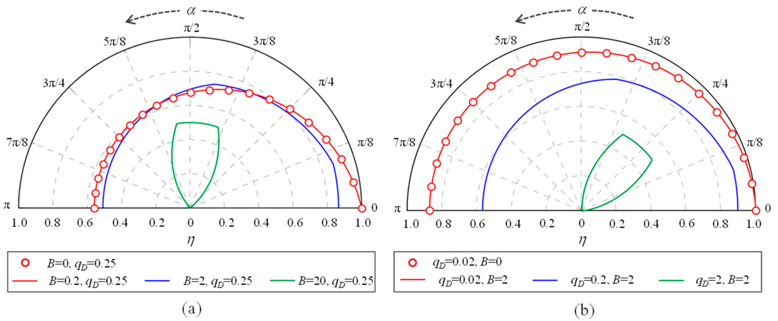
4.3. Dependency of Recirculation Ratios on Parameters

The recirculation ratio of the 1e/2i system, η, depends on the three dimensionless parameters: α, q_D, and B. Figure 8 shows the impact of parameters for 0 ≤ α ≤ π.

When q_D = 0.25 (Figure 8a), the shape of the η-α curve varies with different values of B, where the B value yields the relative distance (b/d) between the two injection wells, 2b. The recirculation ratio is generally larger than 0.5 for a small B value, as indicated by the cases of B = 0.2 and B = 2 in Figure 8a. In particular, when B = 0.2, i.e., when the two injection wells are close to each other, the dependency of the η value on the α value agrees well with the η-α relationship of the 1e/1i system. In comparison, a large B value may cause a decrease in the η value to a range that is generally less than 0.5, especially when the direction of the regional flow (α) is significantly larger or smaller than π/2, as indicated by the case of B = 20 in Figure 8a.

When B = 2 (Figure 8b), the shape of the η-α curve varies with different values of q_D. As indicated, with an increase in the q_D value, the recirculation ratio decreases. It implies that a stronger regional groundwater flow generally leads to a smaller recirculation ratio of the 1e/2i system, which has also revealed from the analytical solution of the 1e/1i system. The η value is higher than 0.5 for a small q_D value, as indicated by the cases of q_D = 0.02 and q_D = 0.2 in Figure 8b. In particular, when q_D = 0.02, i.e., when the regional groundwater flow is relatively weak, the η-α relationship of the 1e/2i system agrees well with that of the 1e/1i system. When the regional groundwater flow is as strong as that in the case of q_D = 2 in Figure 8b, the recirculation ratio of the 1e/2i system is generally less than 0.5, and it may reach 0.5 only when the direction of the regional flow (α) is close to π/4.

4.4. The Impact of Water Table Limitations

Similar to the 1e/1i system, there are also limitations to the water table height in the 1e/2i system. The minimum value of the discharge potential, Φ_ext, can be estimated from the extracting well by substituting X = 2d and Y = r_e into Equation (9), as follows:

$${\Phi }_{\mathrm{ext}}=\frac{1}{2}K{h}_{\mathrm{ref}}^2-q_0\left(2d\cos \alpha +r_e\sin \alpha \right)+\frac{Q}{4\pi }\ln \frac{r_e^2}{\sqrt{\left[4d^2+{(r_e-b)}^2\right]\left[4d^2+{(r_e+b)}^2\right]}}$$

(47)

In practice, this lowest discharge potential should be higher than the threshold of Φ_min, leading to a limitation of q_D:

$$q_D\ge q_{\mathrm{ext}}, q_{\mathrm{ext}}=\frac{q_{0}d\ln \left\{\sqrt{\left[4d^2+{(r_e-b)}^2\right]\left[4d^2+{(r_e+b)}^2\right]}/r_e{}^2\right\}}{K{h}_{\mathrm{ref}}^2-2q_0\left(2d\cos \alpha +r_e\sin \alpha \right)-2{\Phi }_{\min }}$$

(48)

The highest discharge potential may exist within an injection well, either I₁ or I₂. The discharge potentials are denoted as Φ_I1 or Φ_I2, respectively, for I₁ and I₂, and can be estimated from the radius of the injection well (I₁: X = 0, Y₁ = b − r_i; I₂: X = 0, Y₂ = −b + r_i), as follows:

$${\Phi }_{\mathrm{I}1}=\frac{1}{2}K{h}_{\mathrm{ref}}^2-q_0\left(b-r_i\right)\sin \alpha +\frac{Q}{4\pi }\ln \frac{4d^2+{(b-r_i)}^2}{\left|2b{r}_i-r_i^2\right|}$$

(49)

$${\Phi }_{\mathrm{I}2}=\frac{1}{2}K{h}_{\mathrm{ref}}^2-q_0\left(-b+r_i\right)\sin \alpha +\frac{Q}{4\pi }\ln \frac{4d^2+{(b-r_i)}^2}{\left|2b{r}_i-r_i^2\right|}$$

(50)

In practice, the highest discharge potential should be less than Φ_max, leading to the following limitations:

$$q_D\ge q_{\mathrm{I}1}, q_{\mathrm{I}1}=\frac{d{q}_0\ln [(4d^2+{(b-r_i)}^2)/\left|2b{r}_i-r_i^2\right|]}{2{\Phi }_{\max }-K{h}_{\mathrm{ref}}^2+2q_0\left(b-r_i\right)\sin \alpha }$$

(51)

$$q_D\ge q_{\mathrm{I}2}, q_{\mathrm{I}2}=\frac{d{q}_0\ln [(4d^2+{(b-r_i)}^2)/\left|2b{r}_i-r_i^2\right|]}{2{\Phi }_{\max }-K{h}_{\mathrm{ref}}^2+2q_0\left(-b+r_i\right)\sin \alpha }$$

(52)

A combined result of the limitations is:

$$q_D\ge q_{\min }, q_{\min }=\max \{q_{\mathrm{ext}},q_{\mathrm{I}1},q_{\mathrm{I}2}\}$$

(53)

As indicated in Figure 8b, the recirculation ratio of the 1e/2i system generally decreases with the increasing value of q_D. Thus, the limitation of q_D given in Equation (53) generally leads to a maximum threshold of the recirculation ratio, η_c, which is determined by q_min.

5. Comparison Analyses and Discussions on a Synthetic Example

5.1. Hydrogeological Conditions

In this section, we compare the development of RZs and the recirculation ratio of the PAT system between the 1e/1i and 1e/2i systems for a synthetic example of satisfying physical experiences in practice. The properties of the aquifer-well system in the synthetic example are listed in

Table 1. Settings of the synthetic example.

Theme	Elements and Parameters	Symbol	Value
Aquifer conditions	Hydraulic conductivity of the aquifer	K	5 m/d
	Regional groundwater flow rate	q0	0.075 m2/d
	Regional groundwater flow direction	α	0 ≤ α ≤ π
	Ground surface elevation	zsurf	20 m
	Aquifer bottom elevation	zbot	0 m
	Initial water level at (x = 0, y = 0)	href	15 m
Water level limitations	Allowed highest water level	hmax	18 m
	Maximum discharge potential	Φmax	810 m3/d
	Allowed lowest water level	hmin	10 m
	Minimum discharge potential	Φmin	250 m3/d
Wells	Location of the extraction well	d	20 m
	Well radius	re = ri	0.1 m
	Half the distance between injection wells	b	≤20 m
	Flow rate of the extraction well	Q	<1000 m3/d

. The regional groundwater flow rate, q₀ = 0.075 m²/d, is specified for a condition in which the natural hydraulic gradient is 0.1%.

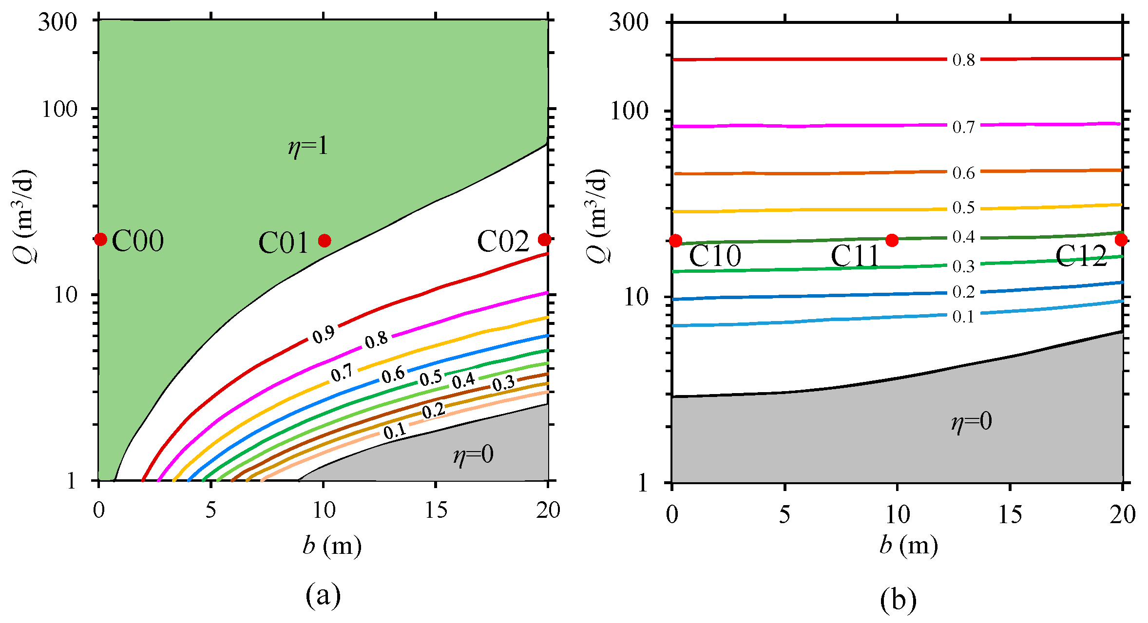
5.2. RZs and Recirculation Ratios When α = 0 and α = π

Regional groundwater flow scenarios of α = 0 and α = π are particularly investigated for the synthetic example in this section to observe results in a special condition: the regional flow is parallel to the arrangement line (the X axis) of wells. For both scenarios, three cases are typically selected to observe the patterns of the RZs, as listed in

Table 2. Typical cases for scenarios of α = 0 and α = π.

Scenario	PAT System	Cases	b (m)	qmin	Qmax (m3/d)	Q (m3/d)	η
α = 0	1e/1i system	C00	0	0.0365	258	20	0
	1e/2i system	C01	10	0.0292	323	20	0
	1e/2i system	C02	20	0.0296	319	20	0.93
α = π	1e/1i system	C10	0	0.0285	258	20	0.41
	1e/2i system	C11	10	0.0286	329	20	0.40
	1e/2i system	C12	20	0.0290	325	20	0.38

. The 1e/1i system is used in cases C00 and C10 to compare the 1e/2i system used in cases C01, C02, C11, and C12. When the 1e/1i system is used, the values of q_ext and q_inj are estimated with Equation (24) and Equation (26), respectively. Then the value of q_min is determined according to Equation (27). It yields the maximum allowable flow rate of the extraction well, which is denoted as Q_max (=2πdq₀/q_min). Similarly, the values of q_min and Q_max can be determined with Equation (53) when the 1e/2i system is used. The results of these threshold values are also given in Table 2. In comparison to the 1e/1i system, it is clear that the 1e/2i system has a higher allowable pumping rate. For instance, the Q_max values in the C01 and C11 cases are ~25% higher than those in the C00 and C10 cases. Patterns of RZs for these cases are shown in Figure 9. Only one RZ is developed in the cases of the 1e/1i system, shown as zone III in Figure 9a for the case C00 and Figure 9d for the case C10. Two RZs are developed in the cases of the 1e/2i system, which are definitely symmetrical about the X-axis. When all of the stagnation points (S₁, S₂, and S₃) fall on the X-axis (Figure 9b for the case C01), or two stagnation points fall on the Y-axis and the other one falls on the X-axis (Figure 9e for the case C11 and Figure 9f for the case C12), the two RZs are fully connected by the X-axis. The C02 case (Figure 9c) is special because the two stagnation points, S₂ and S₃ do not fall on the X-axis or Y-axis, and the regional flow reaches the pumping well along a path between S₂ and S₃, i.e., the capture zone of the regional flow toward the pumping well separates the RZs of the two injection wells.

In scenarios of α = 0 or α = π, the recirculation ratio is subject to the distance between injection wells, 2b, and the flow rate of the extraction well, Q. Using analytical solutions in this study, the recirculation ratio is estimated and shown in Figure 10 for both scenarios of α = 0 and α = π. When α = 0, the recirculation ratio (η) ranges between 0 and 1, which generally increases with increasing Q and decreasing b values. As exhibited in Figure 10a, there are two special areas in the b-Q space for η: one yields η = 0 for relatively large η and small Q values (absence of RZs), and another yields η = 1 for relatively small η and large Q values (e.g., cases C00 and C01 in Table 2). When α = π, the η value is positively dominated by the Q value while showing a slight positive dependency on the b value (Figure 10b). There is η = 0, when the Q value is smaller than a threshold (gray area in Figure 10b), while η cannot reach 1 even when Q is close to Q_max (Table 2, ~300 m³/d), because the regional flow must be partially captured by the pumping well in the scenarios of α = π.

5.3. Sensitivity to the Angle of Regional Groundwater Flow

The impact of α on the recirculation ratio and RZs is investigated on the basis of the cases listed in Table 2 by fixing Q = 20 m³/d for b = 0 m (1e/1i system), b = 10 m, or 20 m (1e/2i system), while changing the α value. This value of Q is lower than the maximum allowable pumping rate and falls on the moderate side of the b-Q space for the recirculation ratio (Figure 10); thus, it is suitable for investigating the general role of the regional flow angle.

The dependence of the recirculation ratio on the angle of regional flow is shown in Figure 11. For the 1e/1i system (b = 0 m), the η value decreases from 1 to 0.40 when the α value increases from 0 to π. The data points of this 1e/1i system in Figure 11 approximately fall on the changing curve of the 1e/2i system with b = 10 m. It indicates that the dependencies of η on α for the 1e/2i system of b = 10 m and the 1e/1i system are quite similar. However, the obvious difference between the 1e/1i system and the 1e/2i system can be seen when b = 20 m. When the α value ranges between 0.17π and 0.61π, the recirculation ratio of the 1e/2i system is higher than that of the 1e/1i system. Otherwise, in the ranges of 0 ≤ α < 0.17π and 0.61π < α ≤ π, the recirculation ratio of the 1e/2i system is lower than that of the 1e/1i system.

Patterns of RZs in different cases with typical angles of regional flow are shown in Figure 12 and Figure 13 for b = 10 m and b = 20 m, respectively. The α values of these cases include the critical points (α = 0.17π and α = 0.61π) of α-η curves in Figure 11 and two transition points (α = 0.03π and α = 0.3π). As indicated in Figure 12, the double RZs in cases of b = 10 m are always adjacent, with a border streamline between the stagnation S₂ and the extraction well. When the α value increases from 0.03π (Figure 12a) to 0.17π (Figure 12b) and then increases to 0.3π and 0.61π, more and more regional flow is captured by the extraction well, with increasing width of the capture zone. This response causes a decrease in flow rate in RZs and then reduces the recirculation ratio. Similar patterns exist in cases where b = 10 m, as shown in Figure 13. However, a new pathway of the regional flow captured by the extraction well emerges in places between the two injection wells when α = 0.03π (Figure 13a) and α = 0.17π (Figure 13b). This new pathway does not exist when α = 0.3π (Figure 13c) and α = 0.61π (Figure 13d), leading to quite similar capture zones in comparison to those of b = 10 m.

6. Conclusion Remarks

We obtain analytical solutions of RZs and recirculation ratios for two kinds of the PAT system in an unconfined aquifer influenced by regional groundwater flow. An arbitrary direction of the regional flow as well as the impact of water table limitations in the extraction and injection wells are considered. The major conclusions can be summarized as follows:

(1)

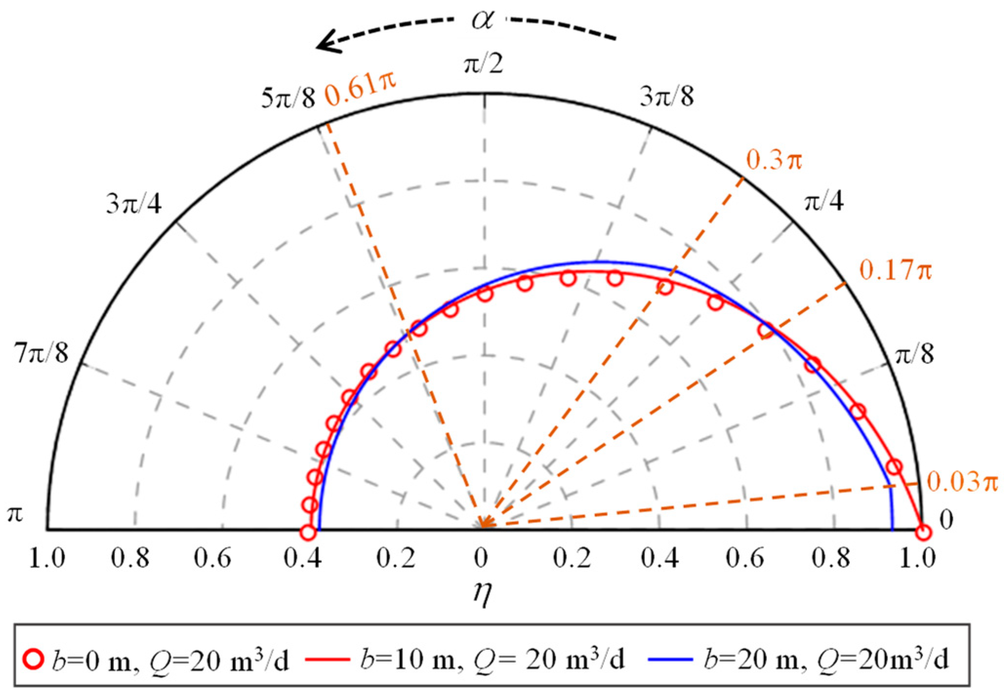
For the 1e/1i system, the existence of the RZ and the recirculation ratio (η) depend on the angle (α) and relative rate (q_D) of the regional flow. When the direction of the regional flow is close to the path from the injection well to the extraction well (α ≈ 0), the RZ exists with a η value that is close to 1. Larger q_D and α values generally lead to smaller η value;

(2)

For the 1e/2i system, the patterns of RZs and the recirculation ratio depend on α, q_D and the relative distance between the two injection wells (B). The 1e/2i system is equal to the 1e/1i system when B = 0. In general, an increase in the B value may reduce the integrity of RZs or take away one or two RZs and lead to a decrease in the recirculation ratio, especially when α is close to 0 or π;

(3)

Water table limitations in the extraction and injection wells yield a maximum allowable pumping rate for the PAT system and then lead to an upper bound on the recirculation ratio. The 1e/2i system generally has a higher allowable pumping rate than the 1e/1i system;

(4)

A special zone of α may exist for the sake of producing RZs in the 1e/2i system, even leading to a larger recirculation ratio than that of the 1e/1i system.

Assumptions and simplifications are introduced in this study to obtain analytical solutions, which limit the applicability of the study results and should be carefully considered in practice. In Section 2.1, five major simplifications were listed that are necessary for using the analytical solutions of RZs and the recirculation ratio. In the real world, groundwater flow around the wells at the beginning of a PAT system may follow a significantly unsteady pattern, which does not satisfy the steady-state flow assumption in this study. Thus, our research results are more suitable to assess the long-term behavior of a PAT system with relatively steady performance. Although we only considered one or two injection wells, PAT systems with more than two injection wells or with multiple extraction wells generally have similar behaviors as those discovered in this study. Further investigations are expected to reveal details of different recirculation zones among different extraction wells in the same field.

References

1. Truex, M.; Johnson, C.; Macbeth, T.; Becker, D.; Lynch, K.; Giaudrone, D.; Frantz, A.; Lee, H. Performance Assessment of Pump-and-Treat Systems. Groundw. Monit. Rem. 2017, 37, 28–44. [Google Scholar] [CrossRef]
2. Yuan, F.; Zhang, J.; Chen, J.; Chen, H.; Samuel, B. In Situ Pumping-Injection Remediation of Strong Acid-High Salt Groundwater: Displacement-Neutralization Mechanism and Influence of Pore Blocking. Water 2022, 14, 2720. [Google Scholar] [CrossRef]
3. Mackay, D.M.; Cherry, J.A. Groundwater contamination: Pump-and-treat remediation. Environ. Sci. Technol. 1989, 23, 630–636. [Google Scholar] [CrossRef]
4. Bedient, P.B.; Rifai, H.S.; Newell, C.J. Ground Water Contamination: Transport and Remediation; Prentice-Hall International: Englewood Cliffs, NJ, USA, 1994; pp. 395–450. [Google Scholar]
5. Bear, J.; Sun, Y.W. Optimization of pump-treat-inject (PTI) design for the remediation of a contaminated aquifer: Multi-stage design with chance constraints. J. Contam. Hydrol. 1998, 29, 225–244. [Google Scholar] [CrossRef]
6. Chang, L.C.; Chu, H.J.; Hsiao, C.T. Optimal planning of a dynamic pump-treat-inject groundwater remediation system. J. Hydrol. 2007, 342, 295–304. [Google Scholar] [CrossRef]
7. Bear, J.; Cheng, A.H.-D. Modeling Groundwater Flow and Contaminant Transport; Springer Science & Business Media: Berlin/Heidelberg, Germany, 2010; pp. 516–519. [Google Scholar]
8. Sdai, M.A. Well rate and placement for optimal groundwater remediation design with a surrogate model. Water 2019, 11, 2233. [Google Scholar] [CrossRef] [Green Version]
9. Goltz, M.N.; Christ, J.A. Recirculation Systems, Delivery and Mixing in the Subsurface: Processes and Design Principles for In Situ Remediation; Springer: Cham, Switzerland, 2012; pp. 139–168. [Google Scholar]
10. Sheahan, N.T. Injection/Extraction Well System—A Unique Seawater Intrusion Barriera. Groundwater 1977, 15, 32–50. [Google Scholar] [CrossRef]
11. Lu, C.; Werner, A.D.; Simmons, C.T.; Robinson, N.I.; Luo, J. Maximizing Net Extraction Using an Injection-Extraction Well Pair in a Coastal Aquifer. Groundwater 2013, 51, 219–228. [Google Scholar] [CrossRef]
12. Shi, L.; Lu, C.; Ye, Y.; Xie, Y.; Wu, J. Evaluation of the performance of multiple-well hydraulic barriers on enhancing groundwater extraction in a coastal aquifer. Adv. Water Resour. 2020, 144, 103704. [Google Scholar] [CrossRef]
13. Grove, D.B.; Beetem, W.A. Porosity and Dispersion Constant Calculations for a Fractured Carbonate Aquifer Using the Two Well Tracer Method. Water Resour Res. 1971, 7, 128–134. [Google Scholar] [CrossRef]
14. Clement, T.P.; Truex, M.J.; Hooker, B.S. Two-Well Test Method for Determining Hydraulic Properties of Aquifers. Groundwater 1997, 35, 698–703. [Google Scholar] [CrossRef]
15. Gringarten, A.C.; Sauty, J.P. A theoretical study of heat extraction from aquifers with uniform regional flow. J. Geophys. Res. 1975, 80, 4956–4962. [Google Scholar] [CrossRef]
16. Wu, B.; Zhang, X.; Jeffrey, R.G.; Bunger, A.P.; Jia, S. A simplified model for heat extraction by circulating fluid through a closed-loop multiple-fracture enhanced geothermal system. Appl. Energy 2016, 183, 1664–1681. [Google Scholar] [CrossRef]
17. Wu, B.; Zhang, G.; Zhang, X.; Jeffrey, R.G.; Kear, J.; Zhao, T. Semi-analytical model for a geothermal system considering the effect of areal flow between dipole wells on heat extraction. Energy 2017, 138, 290–305. [Google Scholar] [CrossRef]
18. Bear, J. Hydraulics of Ground Water; McGraw-Hill: New York, NY, USA, 1979; pp. 367–374. [Google Scholar]
19. Dacosta, J.; Bennett, R. The pattern of flow in the vicinity of a recharging and discharging pair of wells in an aquifer having areal parallel flow. Int. Ass. Sci. Hydrol. Publ. 1960, 52, 524–536. [Google Scholar]
20. Suk, H.; Chen, J.S.; Park, E.; Han, W.S.; Kihm, Y.H. Numerical evaluation of the performance of injection/extraction well pair operation strategies with temporally variable injection/pumping rates. J. Hydrol. 2021, 598, 126494. [Google Scholar] [CrossRef]
21. Bumb, A.C.; Mitchell, J.T.; Gifford, S.K. Design of a ground-water extraction /reinjection system at a superfund site using MODFLOW. Ground Water 1997, 35, 400–408. [Google Scholar] [CrossRef]
22. Zhan, H.B. Analytical and numerical modeling of a double well capture zone. Math Geol. 1999, 31, 175–193. [Google Scholar] [CrossRef]
23. Li, H.; Wang, X.S. A Preliminary Study on a Pumping Well Capturing Groundwater in an Unconfined Aquifer with Mountain-Front Recharge from Segmental Inflow. Water 2019, 11, 1243. [Google Scholar] [CrossRef] [Green Version]
24. Satkin, R.L.; Bedient, P.B. Effectiveness of various aquifer restoration schemes under variable hydrogeologic conditions. Groundwater 1988, 26, 488–498. [Google Scholar] [CrossRef]
25. Christ, J.A.; Goltz, M.N.; Huang, J.Q. Development and application of an analytical model to aid design and implementation of in situ remediation technologies. J. Contam. Hydrol. 1999, 37, 295–317. [Google Scholar] [CrossRef]
26. Cunningham, J.A.; Reinhard, M. Injection-extraction treatment well pairs: An alternative to permeable reactive barriers. Groundwater 2002, 40, 599–607. [Google Scholar] [CrossRef] [PubMed]
27. Shan, C. An analytical solution for the capture zone of two arbitrarily located wells. J. Hydrol. 1999, 222, 123–128. [Google Scholar] [CrossRef]
28. Luo, J.; Kitanidis, P.K. Fluid residence times within a recirculation zone created by an extraction-injection well pair. J. Hydrol. 2004, 295, 149–162. [Google Scholar] [CrossRef]
29. Samani, N.; Zarei-Doudeji, S. A General Analytical Capture Zone model: A Tool for Groundwater Remediation. In Proceedings of the 8th Vienna International Conference on Mathematical Modelling, Vienna, Austria, 18–20 February 2015; pp. 234–239. [Google Scholar] [CrossRef]
30. Christ, J.A.; Goltz, M.N. Hydraulic containment: Analytical and semi-analytical models for capture zone curve delineation. J. Hydrol. 2002, 262, 224–244. [Google Scholar] [CrossRef]
31. Samani, N.; Zarei-Doudeji, S. Capture zone of a multi-well system in confined and unconfined wedge-shaped aquifers. Adv. Water Resour. 2012, 39, 71–84. [Google Scholar] [CrossRef]
32. Fienen, M.N.; Jian, L.; Kitanidis, P.K. Semi-analytical homogeneous anisotropic capture zone delineation. J. Hydrol. 2005, 312, 39–50. [Google Scholar] [CrossRef]
33. Luo, J.; Wu, W.M.; Fienen, M.N.; Jardine, P.M.; Mehlhorn, T.L.; Watson, D.B.; Cirpka, O.A.; Criddle, C.S.; Kitanidis, P.K. A nested-cell approach for in situ remediation. Groundwater 2006, 44, 266–274. [Google Scholar] [CrossRef]
34. Luo, J.; Wu, W.M.; Carley, J.; Ruan, C.; Gu, B.; Jardine, P.M.; Criddle, C.S.; Kitanidis, P.K. Hydraulic performance analysis of a multiple injection-extraction well system. J. Hydrol. 2007, 336, 294–302. [Google Scholar] [CrossRef]
35. Bear, J. Dynamics of Fluids in Porous Media; Dover Publications: New York, NY, USA, 1972; pp. 222–246. [Google Scholar]
36. Strack, O.D.L. Groundwater Mechanics; Prentice Hall: Englewood Cliffs, NJ, USA, 1989; pp. 278–282. [Google Scholar]
37. Campos, L.M.B.D.C. Complex Analysis with Applications to Flows and Fields; CRC press: Boca Raton, FL, USA, 2010; pp. 65–80. [Google Scholar]
38. Holzbecher, E. Streamline Visualization of Potential Flow with Branch Cuts, with Applications to Groundwater. J. Flow Vis. Image Process. 2018, 25, 119–144. [Google Scholar] [CrossRef]
39. Kahan, W. Branch cuts for complex elementary functions. In The State of the Art in Numerical Analyszs; Powell, M.J.D., Iserles, A., Eds.; Oxford University Press: Oxford, UK, 1987; pp. 165–211. [Google Scholar]
40. Sato, K. Complex Analysis for Practical Engineering; Springer: Cham, Switzerland, 2015. [Google Scholar]
Figure 1. Schematic profiles of PAT system: (a) 1e/1i system with one extraction well and one injection well; (b) 1e/2i system with one extraction well and two injection wells named I1 and I2, where RZ1 and RZ2 are recirculation zones of I1 and I2, respectively. Arrows indicate the flow direction.
Water 15 02852 g001
Figure 2. Plane positions of the extraction (E) and injection (I) wells with the Cartesian coordinates: (a) 1e/1i system; (b) 1e/2i system.
Water 15 02852 g002
Figure 3. Jump of the stream function value for a stream line extending across branch cut lines: (a) the impact of a branch cut from an extraction well; (b) joint impacts of branch cut lines from extraction and injection wells. A and P are two points on one stream line. The red, green, or blue solid lines indicate segments with different stream function values on the same streamline.
Water 15 02852 g003
Figure 5. Dependency of the recirculation ratio, η, on the angle (α) and relative rate (qD) of the regional flow for the 1e/1i system.
Water 15 02852 g005
Figure 6. Typical stagnation points and divide lines to infinity of the 1e/2i system. Black arrows indicate the groundwater flow direction of divide lines; red arrows indicate the regional groundwater flow direction; and blue arrows indicate the groundwater flow direction in the middle part of any two divide lines.
Water 15 02852 g006
Figure 8. Dependency curves of recirculation ratio (η) with a for the 1e/2i system: (a) Giving qD = 0.25 while different B values; (b) Giving B = 2 while different qD values. Circles are data points for the 1e/1i system (B = 0).
Water 15 02852 g008
Figure 9. Patterns of RZs for typical cases listed in Table 2: (a) C00; (b) C01; (c) C02; (d) C10; (e) C11; (f) C12. Red zones are the regional flow captured by extraction well E; light blue zone is the regional flow contributed by the injection well I1 in C02, C11 and C12; light green zone is the regional flow contributed by the injection well I2 in C02, C11 and C12; blue zone is the regional flow contributed by the injection well in C01; III1 and III2 are number of RZs for injection well I1 and I2, respectively, and filled with dark blue and dark green; III is the number of RZ in C00 and C10, and filled with green. Arrows indicate groundwater flow direction.
Water 15 02852 g009
Figure 10. Dependency of the recirculation ratio on b and Q for scenarios of 1e/2i system: (a) α = 0; (b) α = π. Red circles denote the cases in Table 2. The vertical coordinate is labeled with the logarithmic scale to clearly show patterns for small Q values.
Water 15 02852 g010
Figure 11. Dependency of the recirculation ratio (η) on the angle of regional flow (α) for scenarios of Q = 20 m3/d with b = 0 m, b = 10 m and b = 20 m.
Water 15 02852 g011
Figure 12. RZs patterns of 1e/2i system with b = 10 m and Q = 20 m3/d for typical angles of the regional flow: (a) α = 0.03π; (b) α = 0.17π; (c) α = 0.3π; (d) α = 0.61π. Red zones are the regional flow captured by the extraction well E; light blue zone is the regional flow contributed by the injection well I1; light green zone is the regional flow contributed by the injection well I2; III1 and III2 are number of RZs for injection well I1 and I2, respectively, and filled with dark blue and dark green. Arrows indicate groundwater flow direction.
Water 15 02852 g012
Figure 13. RZs patterns of 1e/2i system with b = 20 m and Q = 20 m3/d for typical angles of the regional flow: (a) α = 0.03π; (b) α = 0.17π; (c) α = 0.3π; (d) α = 0.61π. Red zones are the regional flow captured by extraction well E; light blue zone is the regional flow contributed by the injection well I1; light green zone is the regional flow contributed by the injection well I2; III1 and III2 are number of RZs for injection well I1 and I2, respectively, and filled with dark blue and dark green;. Arrows indicate groundwater flow direction.
Water 15 02852 g013