Statistical Analysis of the Wave Runup at Walls in a Changing Climate by Means of Image Clustering

Abstract

This contribution builds on an existing methodology of image clustering analysis, conceived for modelling the wave overtopping at dikes from video records of laboratory experiments. It presents new procedures and algorithms developed to extend this methodology to the representation of the wave runup at crown walls on top of smooth berms. The upgraded methodology overcomes the perspective distortion of the native images and deals with the unsteady, turbulent and bi-phase flow dynamics characterizing the wave impacts at the walls. It accurately reconstructs the free surface along the whole structure profile and allows for a statistical analysis of the wave runup in the time and spatial domain. The effects of different structural configurations are investigated to provide key information for the design of coastal defences. In particular, the effects of increased sea levels in climate change scenarios are analysed. Innovative results, such as profiling of the envelopes of the runup along the wall cross and front sections, and the evidencing of 3D effects on the runup are presented. The extreme runup is estimated for the definition of the design conditions, while the envelopes of the average and minimum runup heights are calculated to assess the normal exercise conditions of existing structures.

1. Introduction

Coastal areas, dealing with sea-level rise and facing storms of increasing severity and frequency, are already experiencing the effects of global climate change. Indeed, despite the lack of understanding of the systematic and long-term trends of climate change in waves [1,2], evidence is available that extreme wave heights have increased in the South and North Atlantic Oceans by around 0.8 cm/year over the period 1985–2018 [3]. Furthermore, high-confidence projections of increased significant wave heights across the Southern Ocean, the tropical eastern Pacific and the Baltic Sea have been estimated [3]. The enhancement of wave heights contributes to generating or emphasising extreme sea-level events, coastal erosion and flooding.

Furthermore, it is nowadays well established that the global mean sea level is rising [4], with acceleration in recent decades due to increasing rates of ice loss from the Greenland and Antarctic ice sheets, as well as continued glacier mass loss and ocean thermal expansion [3]. Between 1902 and 2015, global sea level rose by 16 cm [3] and many coastal regions are projected to face a global sea-level rise of 0.5–2 m by the year 2100. Sea-level rise is already causing increased coastal flooding [5], and it is expected that upper-end sea-level rise scenarios could displace hundreds of millions of people by the end of the 21st century [6].

Coastal flooding is caused by astronomic tides, storm surge and waves. Apart from the contribution of tides, climate-change induced phenomena such as sea-level rise, increasing violent storm conditions and extreme waves all contribute to exacerbating the maximum elevation reached by the wave motion on beaches and on coastal structures, i.e., the wave runup [7,8,9]. Many coastal structures built in the past may therefore be inadequate for the predicted increased runup heights and may require upgrading. A standard practice for upgrading the hydraulic performance of coastal defences is to include crown walls on top of existing breakwaters, dikes or berms with or without overhanging parts, such as parapets or bullnoses (inter alia, [10,11,12]). Despite a number of studies detailing the structural performance of crown walls and parapets [12,13,14,15,16], to the best of the authors’ knowledge, no method exists to predict wave runup at these structure types. Nevertheless, quantifying the wave runup and its evolution with respect to past decades and predicting its progress in the near future is a key aspect to consider when designing new coastal protections or planning the management of existing defences.

Historically, studies on wave runup were carried out through physical modelling exercises using step gauges, resistant gauges and resistant probes (e.g., [17,18]). On the one hand, all these techniques suffer from large disturbances induced by turbulence and the aeration of the flow, making measurements very difficult to interpret [19]; on the other hand, they may cause significant disturbances to the measurements themselves, as in the case of the large-scale tests performed by Van der Meer et al. [18] with streamlined floaters on the water, which gave accurate measurements of the wave runup but interacted with the overtopping flow due to their considerable dimensions.

Since the 2010s, the use of video imagery has been increasingly recognised as an efficient technique to estimate wave runup, overcoming some of the limitations imposed by physical measurements. Blenkinsopp et al. [20], Vousdoukas et al. [21] and Almeida et al. [22] made use of laser-scanner techniques to measure the free-surface elevations in the swash zone and reconstruct the position of the shoreline over time. Hofland et al. [19] measured the wave runup height on a dike slope with a laser scanner, while Almar et al. [23] introduced and validated the use of the Radon transform to detect the instantaneous position of the shoreline from uprush and backwash on a beach based on the coastal image data collected by monitoring systems such as ARGUS [24,25]. Den Bieman et al. [26] used segmentation algorithms to obtain quantitative measurements of the free surface elevation and of the wave runup from the video analysis of physical model tests. In recent years, the diffusion of high-resolution cameras and of sophisticated algorithms for image processing has allowed the obtainment of coastal indicators such as shoreline position and wave runup with adequate spatial accuracy and high temporal resolution [27]. All these studies illustrate and demonstrate the effectiveness and advantages of video imagery as a technique to model wave runup with respect to more traditional techniques.

Starting from the abovementioned lack of information on the wave runup at crown walls and parapets and following the stream of machine-learning techniques for reconstructing quantitative data from video imagery, this contribution presents the extension of an existing methodology of image clustering analysis to represent and quantify, for the first time, the wave runup at crown walls installed on top of coastal defences. Exploiting the potential of the image clustering analysis, the novel part of the methodology offers the possibility to derive a fully space-time statistical analysis of the wave runup at crown walls. The main goal is to provide practical information for (i) the assessment of the hydraulic performance of the walls in exercise conditions and for (ii) the design of new defences and for the upgrade of existing ones to account for climate change scenarios. For this purpose, different structural configurations under climate change scenarios were analysed and processed with the new methodology, resulting in a parametrization of the effects of the most relevant geometric parameters on the wave runup.

The proposed study is based on the extension of an existing methodology of image clustering analysis developed by the authors for the representation of the wave overtopping at dikes [28]. The methodology is applied here to the analysis of video records of eight tests of wave overtopping and wave impacts at smooth berms, taken from a set of lab experiments conducted and filmed by Formentin et al. [16] (Section 2). The existing methodology was upgraded with the introduction of new procedures (Section 3) to extend the detection of the free-surface elevation to the crown wall area and optimize the reconstruction of the profiles of the water up-rushing the walls (Section 4). The free-surface data were further analysed to extract the wave runup values and the results of the statistical and parametric analysis carried out are illustrated and discussed (Section 5). Finally, a few concluding remarks, illustrating potentialities and limits of the methodology, are made (Section 6).

2. Tests and Laboratory Setup

The new part of the methodology of video cluster analysis proposed in this contribution was applied to a subset of 8 experiments selected among 128 tests of wave overtopping and wave loads carried out against smooth dikes with crown wall structures in the wave flume of the Hydraulic Laboratory of the University of Bologna (Unibo). These tests, consisting of irregular wave attacks carried out against various configurations of the same basic structures characterized by a plain, trapezoidal cross section, are described in detail in [16,29]. The scheme of the tested cross sections is shown in Figure 1, where the following symbols are used: h is the water depth at the wave-maker and before the dike toe; cot(α_d) is the structure slope; B is the width of the dike crest that, following the EurOtop [30] manual classification of the structure types, is schematized as a berm and will be referenced as such hereinafter; h_c is the structure height, which was 0.35 m for all the tests; h_w is the height of the crown wall; h_n and ε = 30° are, respectively, the height and the angle of inclination of the parapet which was included on top of the crown wall in some of the tests; h_b is the berm submergence, with h_b < 0 and h_b > 0 for emerged and submerged berm, respectively; R_c is the structure total freeboard, calculated from the top of the crown wall to the still water level, R_c = h_w − h_b; H_s is the significant wave height and L_m−1,0 is the spectral wave length characterizing the incident waves and γ_f is the factor representing the roughness of the structures according to EurOtop [30]. Since all the parts of the structures were formed in plexiglass, γ_f = 1.

The variety of the tested configurations in the lab was obtained by varying: the dike slope, cot(α_d) = 2 and 4; the berm width, B = 0.15 and 0.30 m; the berm relative emergence to the wave height, h_b/H_s = 0, and −0.5; the crown wall height, h_w = 0.04 and 0.05 m and the presence or not of the parapet. Each configuration was subjected to the following 4 target wave conditions: H_s = 0.05 m and s_m−1,0 = H_s/L_m−1,0 = 0.03; H_s = 0.05 m and s_m−1,0 = 0.04; H_s = 0.06 m and s_m−1,0 = 0.03 and H_s = 0.06 m and s_m−1,0 = 0.04, where s_m−1,0 is the wave steepness. The wave attacks were all characterized by Jonswap spectra, with a peak enhancement factor of γ = 3.3 and consisted of approximately 500–600 waves (according to the target peak wave period, T_p).

The characteristics of the 8 selected tests are reported in

Table 1. Summary of the 8 experiments elaborated with the video cluster analysis. The parameters modified with respect to the benchmark case are highlighted with blue colour. All the 8 different structure configurations were subjected to the same wave attack (target values of H_s = 0.05 m and s_m−1,0 = 0.03) and are characterized by the same berm width B = 0.30 m.

Test ID	cot(αd) [−]	h [m]	hw [m]	hb/Hs [−]	Parapet
TW1	4	0.350	0.05	0	-
TW2	4	0.350	0.04	0	-
TW3	4	0.325	0.05	0.5	-
TW4	4	0.350	0.05	0	Yes
TW5	2	0.350	0.05	0	-
TW6	2	0.350	0.04	0	-
TW7	2	0.325	0.05	0.5	-
TW8	2	0.350	0.05	0	yes

, where the notation introduced in Figure 1 are adopted. The selected tests represent 8 different structural configurations which were set up starting from a benchmark case—characterized by h_w = 0.05 m, h_b/H_s = 0 and no parapet—and by modifying one parameter at once to separately investigate the effects of:

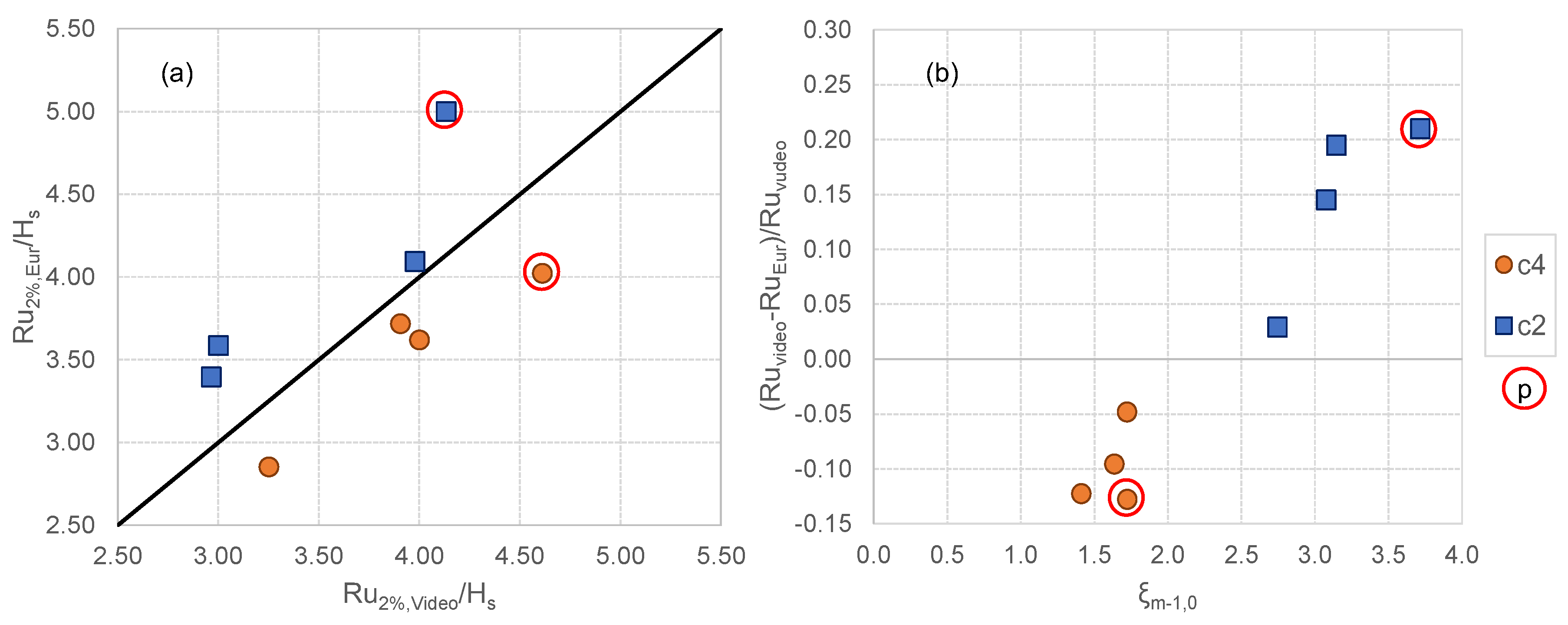
• Different wave-breaking conditions, obtained by selecting both cot(α_d) = 4 and 2; the two slopes, which will be referred as “c4” and “c2” hereinafter, were set up in the lab to determine, respectively, spilling breaker types, with values of the Iribarren–Battjes’ breaker parameter ξ_m−1,0 in the range 1.41–1.72 and plunging breakers, with ξ_m−1,0 = 3.03–3.72. For each test, ξ_m−1,0 was calculated at the toe of the structure based on the values of H_s and L_m−1,0 measured in the wave channel;
• The wall heights, by reducing h_w from 0.05 to 0.04 m;
• The berm relative submergence, by introducing the condition of emerged berm with h_b/H_s = −0.5;
• The parapet.

One single-wave attack (H_s = 0.05 m and s_m−1,0 = 0.03) was selected for all the 8 tests, because it was already observed [16,29] that changing the wave height and the wave period involves scale effects purely; contextually, the adoption of the same wave attack makes the sensitivity analysis to the effects of the different geometrical parameters meaningful. Finally, all the 8 selected configurations involve the same condition of B = 0.30 m.

The details about the instrumentation adopted in the laboratory are given in [28]. The video records of the experiments were performed through a 30 Hz full-HD camera (resolution 1080 × 1920 pixels) placed to the side of the wave flume and perpendicular to it, with the camera lens focusing exactly on the mid-width section of the berm and at the elevation of its crest. Figure 4 shows the camera framing window, with reference to the focus of the camera. The framing window within the glass-sided flume facilitated the filming of the wave–structure interaction processes. Specifically, it was set up to film the wave runup over the dike slope and capture the wave breaking, the flow over the berm, the wave impacts at the walls, the wave runup at the walls and the wave overtopping beyond them. The camera was installed inside a “darkroom” specifically established to enclose the wave flume in the filming area in order to optimize the light condition and to avoid the disturbance of external objects.

3. The Video Cluster Methodology

3.1. Description of the Methodology

The image-processing methodology referenced in the present contribution was developed by Formentin et al. [28] on the basis of the video records of the experiments conducted at Unibo and recalled in Section 2. The core of such a methodology is represented by the application of an image clustering technique [31] to automatically detect significant “features” from the images of the experiments. The open-source toolbox “PRTools” (Pattern recognition Tools, http://prtools.tudelft.nl/?from=www.website80.com, [32]) developed by TU Delft was adopted for the cluster analysis and the features extraction from the videos. The raw outputs of the image clustering are the clustered maps of each single frame of the video record of each experiment. In the clustered maps, the different features “water”, “air” and “structure” are detected and labelled. An example of clustered map reproducing a wave overtopping event is given in Figure 2a, where the different colours identify the different classes of objects (magenta for air, violet for structure, etc.). The image clustering phase is respectively preceded and followed by a number of pre- and post-processing techniques specifically designed to improve the automatic detection phase.

The existing methodology has so far been applied to the application of the image clustering technique in the area of the structure included between the dike slope and the berm, excluding therefore the part with the crown walls. It involves two sets of procedures which elaborate the raw outputs to (i) perform the free-surface tracking and (ii) estimate the number of air bubbles entrapped in the liquid phase. Figure 2b shows the profile of the free surface obtained with the application of the existing procedure to the cluster map of Figure 2a. With the first set of procedures, the instantaneous values of the free-surface elevation are further manipulated to obtain the wave overtopping depths, velocities, volumes and discharges characterizing the flow above the crest of the structures. The second set of procedures is dedicated to the estimation of the number of air bubbles entrapped in the liquid phase during the several phases of the runup and overtopping propagation flow.

The novel part of the methodology presented in this contribution consists in:

• the extension of the existing procedure to the area including the crown walls placed at the inshore edge of the berm and beyond; such extension involves: (i) the adaptation of the pre-clustering techniques to deal with the presence of the wall, (ii) the adaptation of the procedure for the detection of the free surface to the area including the walls and (iii) the elimination of the 3D effects affecting the pictures in the area around the walls;
• a package of new procedures is developed to further manipulate the free-surface elevation in order to extract the following new quantitative data: (i) the wave runup height at the walls, (ii) the number of overtopping waves behind the crown wall and (iii) the number of the wave impacts at the walls.

The conceptual scheme of the whole methodology is illustrated in Figure 3, where the existing and the new parts are distinguished. This figure synthetizes and briefly describes the several steps of the methodology. The details about the existing pre- and post-clustering and the clustering itself are given in Formentin et al. [28].

3.2. Setup of the Virtual Gauges

The new methodology includes several novel aspects related to the elaborations of the free-surface elevation (h, hereinafter) in specific points of the framing window, which will be referenced hereinafter as “virtual wave gauges” (WGs). The positions of these WGs are given in Figure 4 representing the framing window of the camera used to record the experiments. Figure 4 gives reference to the direction and orientation of the horizontal x-axis, to the vertical z-axis and to the position of the origin of the coordinate system (x = 0, z = 0) The y-axis—not shown in the figure—will be used in the present contribution to refer to the third dimension perpendicular to the plane of the frame.

WG1 and WG2 are the two virtual gauges installed above the structure berm and adopted to reconstruct the single overtopping waves over the berm and the number of the impact events at the walls and to estimate the celerity of propagation of the overtopping waves above the berm. WG3 is placed behind the crown wall, and it is used to calculate the number of the waves overtopping the wall. P1, P2 and P3 are the “virtual pressure transducers” and are placed exactly in correspondence of the homonymous real pressure transducers installed in the lab. In Figure 4, the local coordinates of the WGs and of other peculiar points delimiting the areas of the camera framing window dedicated to the free-surface detection, the air entrainment estimation (not shown here), the wave runup and the wave impacts detection are indicated in red and denoted by the symbol “x_i”. These x-values represent the abscissas of these points calculated with respect to the left-most section of the frame. These x-values may vary by ±20 mm depending on the structure slope (c2 or c4), on the crown wall height and random uncertainty. Indeed, it should be noted that—though the camera was always kept in the same position from the beginning to the end of the lab tests—small movements may have occurred due to the routine operation of the system (camera turning on and off, battery recharge, etc.). For this reason, the calibration of the camera was repeated daily, see [28].

The new procedures of the methodology developed to reconstruct the wave runup are described in detail in Section 4. The procedures dedicated to the evaluation of the number of the wave impacts at the walls and of the overtopping waves behind the walls will be part of a separate contribution presently under preparation.

3.3. Accuracy of the Methodology

The accuracy of the whole methodology is primarily determined by the accuracy in the camera calibration process and the related correction of the image distortion. The accuracy in the camera calibration is a direct indicator of the error associated to the h-values and, by extension, to all the quantities representing lengths or heights which are directly computed from h, i.e., the flow depths at WG1 and WG2, the runup heights, the height of the water columns in front of P1, P2 and P3 and the depth of the overtopping flow behind the wall. Similarly to Gaeta et al. [31] and Formentin et al. [28], the calibration was performed following the approach indicated by Bouguet et al. [33] and the accuracy of the camera calibration error was calculated by selecting a sample frame for validation for each experiment, and by comparing the main geometrical distances (e.g., width of the berm or slope angle of the dike) of the picture to the corresponding real-world dimensions obtained after the application of the rotation matrix and translation vector. Following this approach, the relative errors characterizing the length of the berm (B) and the inclination of the dike slope (cotα_d) were calculated for each of the eight selected tests and are shown in

Table 2. Relative errors in the estimation of the length of the berm (B) and the inclination of the dike slope (cotα_d) and mean reprojection error (MRPE) per image resulting from the camera calibration.

Test ID	MRPE [Pixels]	Rel. Error B [−]	Rel. Error cotαd [−]
TW1	2.21	0.08	0.025
TW2	3.05	0.09	0.01
TW3	2.21	0.04	0.06
TW4	1.92	0.08	0.03
TW5	1.11	0.06	0.04
TW6	5.09	0.06	0.02
TW7	1.11	0.04	0.04
TW8	2.73	0.05	0.04

. The following computations were performed:

$$\mathrm{Rel}.\mathrm{Error}B=\frac{{(B}_{real}{-B}_{video})}{B_{real}}$$

(1)

$$\mathrm{Rel}{.\mathrm{Error}\cot \alpha }_d=\frac{({cot\alpha }_d{}_{real}{-cot\alpha }_{d_{video}})}{{cot\alpha }_{d_{real}}},$$

(2)

where B_real and cotα_d,real are the real world values of B and cotα_d and B_video and cotα_d,video are the ones derived from the images. Overall, the relative error of B varies between 4% and 9%, whereas the relative error of cotα varies between 1% and 6%.

The procedure of conversion into real-world coordinates also provides the reprojection error (RPE), i.e., the distance between a pattern key point detected in the calibration image ($\hat{x}$), and a corresponding world point ($\hat{X}$) projected into the same image. Specifically, if P is the projection matrix of the camera and $\hat{x}$ is the image projection of $\hat{X}$ such that $\hat{x}=P·\hat{X}$, the RPE of $\hat{X}$ is the Euclidean distance between $\hat{x}$ and $\hat{X}$.

For each image, its mean reprojection error (MRPE) can be calculated, which can be used as a further indicator of the accuracy of the calibration process:

$$\mathrm{MRPE}=\frac{1}{\mathrm{N}}{{\displaystyle \sum }}_{\mathrm{i}=0}^{\mathrm{N}-1}{\left|\widehat{X_{\mathrm{i}}}{-\hat{x}}_{\mathrm{i}}\right|}_2,$$

(3)

where N is the number of points in the image and $\left|\widehat{X_{\mathrm{i}}}{-\hat{x}}_{\mathrm{i}}\right|$₂ is the Euclidean distance between the i-th real-world and image projected points ${\hat{x}}_i$ and ${\hat{X}}_i$. The values of the MRPE (pixels) obtained for each test are reported in Table 2. By considering an average ratio of pixels/mm of 3.3, it can be estimated that the MRPE per image varies on average between 0.67 and 1.55 mm.

The accuracy of the whole methodology, and therefore the accuracy of the results on the wave runup presented in this contribution (Section 5), is basically determined by the precision of the camera calibration process and by the correction of the image distortion. To these uncertainties, the error propagation related to the application of the several procedures of pattern recognition and automatic detection of the free surface needs to be added. It is not possible to know which is the principal source of error in the model chain, but it is possible to identify all the elements that contribute to the propagation of the error. As reference, Formentin et al. [28] verified the accuracy of the methodology by comparing the results obtained from the imagery of the free-surface elevation with the corresponding laboratory quantities, finding the following relative errors: +36% for the extreme flow depths values; +19% for the average overtopping discharge above the berm; +5% for the estimation of the number of overtopping waves above the berm; +2% for the average and total overtopping volumes over the berm.

As for the wave runup objective of the present contribution, a comparison with methods from the literature is proposed in Section 5.2.

4. Calculation of the Wave Runup

This section details the specific procedures set up for the reconstruction of the wave runup at the crown walls. Such procedure involves the pre-clustering techniques (Section 4.1), the algorithm of automatic detection of the free surface from the clustered model maps of the frames (Section 4.2) and the post-clustering techniques (Section 4.3).

4.1. Adaptation of the Pre-Filtering Techniques

Extending the automatic detection of the free surface to the wall and beyond it means adjusting the procedures to account for the presence of the wall itself and the disturbance it caused to the image clustering. Firstly, as can be appreciated in Figure 2a, the existing methodology is not able to distinguish the wall from the turbulent water jet up rushing over it, since they are both detected as object “air” (magenta colour). To overcome this aspect, it was necessary to tune and modify the pre-clustering filtering techniques by applying a different contrast enhancement technique performing histogram equalization. Such a technique transforms the values of the input image in an intensity image so that the histogram of the output image approximately matches a uniformly distributed histogram. For example, Figure 5 shows the clustered model map (panel c) associated to the frame selected for training the cluster model of test TW5 (panel a), after the application of the new pre-clustering techniques described above (panel b). In Figure 5b, the profile of the wall is enhanced, differently from the real colour image of Figure 5a, where it is completely mixed with the water. As a result, Figure 5c, showing a clustered model map where the profile of the wall is distinguished from the water, differs from Figure 2a.

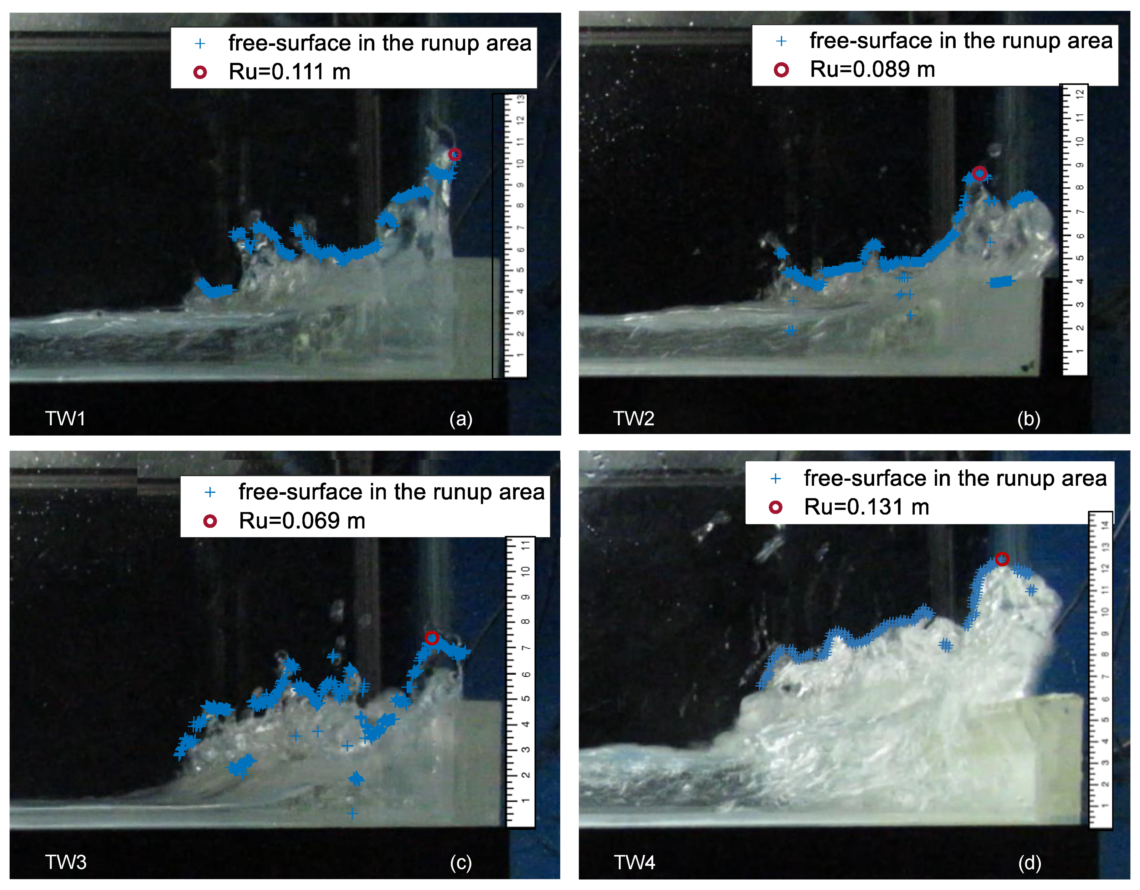
4.2. Extension of the Free-Surface Tracking to the Wall Area

The existing procedure for the free-surface tracking developed by Formentin et al. [28] provides the values of the water depth h above the structure berm, i.e., from x₁ to x_w,1 (see Figure 4). It consists in a customized procedure that, for each frame, takes as input the “edge” of the object “water” detected in the clustered map and returns the effective profile of the free surface, abscissa after abscissa. It is based on the definition of an initial time condition and follows a sort of “forward scheme” to identify the nearby points of the free surface, based on the assumption of the continuity of the free-surface profile itself in time and space. The calculation of the wave runup proposed in this contribution has involved the modification of such existing procedures (see the scheme of Figure 3) to extend the automatic detection of the free-surface tracking from x_w,i to x_w,f (see Figure 4). The new part of the free-surface tracking procedure was kept separated from the existing one to “isolate” the h-values in the runup zone for the specific analyses. It is conceptually subsequent to the existing procedure, because, for each time step, it applies the value of h resulting from the existing procedure as left-boundary condition in x = x_w,i. In case no value is available—for example, because the overtopping flow has not reached the abscissa x_w,i yet—the value h in correspondence of x_w,I is set equal to 0. For x > x_w,i, the new procedure adopts the same forward scheme of the existing one and the same assumption of the continuity of the free-surface profile itself. The procedure includes a control of the h-values that cannot be lower than the wall height (h_w), though the update of the image clustering phase to optimize the pattern recognition and distinguish the water from the wall (Section 4.1) should prevent this shortcoming.

Following this method, the profiles of the up-rushing jets were detected for each frame of each test and the instantaneous values of the wave runup heights, Ru, were calculated as the vertical distances between the highest point reached by the water jet and the still water level [30]. Figure 6 provides an example of the profile of the free surface (blue) circumscribed between x_w,i and x_w,f and the corresponding runup height (red circle) obtained with the new part of the methodology.

Finally, the calculation of the wave runup has involved also the development of a new procedure dedicated to the computation of maximum runup heights of each frame and the extraction of the upper envelopes of the runup profiles over time.

4.3. Perspective Distortion Correction

Figure 4 and Figure 6 show that the wall is strongly affected by a 3D perspectival distortion that, of course, increases radially from the centre (i.e., the focus of the camera) to the sides of the framing window, and therefore it becomes nearly maximum in the horizontal direction in correspondence of the crown wall. The horizontal distortion of the wall due to the perspective effect can be estimated by comparing the difference between x_w,f and x_w,i ≈ 200 mm to the real thickness of the wall, which was 20 mm. Such distortion cannot be corrected with the application of the rotation translation matrix and the translation vectors deriving from the camera calibration process. These transformations are indeed used to convert all the data from the videos of the experiments from intrinsic to world coordinates and can correct the skewness, the tangential distortion and optical errors due to lens distortion. To reduce the perspective effect, a specific procedure of perspective control and correction developed by Chan [34] was included in the step of the calculation of the wave runup at the walls, after the automatic reconstruction of the free-surface elevation (Section 4.2) and before converting the data into real-world coordinates. Figure 7 compares the example free-surface profile obtained in the runup area before (panel a) and after (panel b) the application of the perspective correction. As is evident in panel b, the perspective correction significantly reduces the 3D effect of the wall allowing the reconstruction of the up-rushing jet, but it contextually generates a radial distortion in the image that affects the horizontal distances and would make meaningless all the other elaborations and results. This is the reason why the perspective correction procedure was applied to the reconstruction of the runup only.

5. Statistical and Parametric Analysis of the Wave Runup

Depending on the incident, irregular waves, the Ru-values are stochastic variables varying in time for each overtopping event [30]. Therefore, specific statistics (mean, median, maximum, etc.) are necessary to characterize the distribution of the Ru-values of each test. To this purpose, the probability of exceedance of Ru were derived (Section 5.1) and specific quantiles were calculated for each test. Generally, the literature (e.g., [19,30]) indicates the “2% exceedance wave runup height”, Ru_2%, as a characteristic statistic and design basis for the definition of the crest levels in case of irregular waves. Ru_2% is defined as the wave runup height exceeded by 2% of the incident waves. Other studies (inter alia, [8,35]) refer instead to the maximum wave runup height, Ru_max as a design parameter. In the present study, both the parameters Ru_2%,video and Ru_max,video were calculated from the probability exceedance curves for each test in order to compare the results of the video analysis with those from the literature (Section 5.2).

Finally, it was observed that the instantaneous Ru-values vary also with the cross-shore distance (x) and across the front section of the crown walls due to 3D effects, as it can be appreciated in the example of Figure 8, showing two consecutive overtopping events of the same test reaching two different Ru-values (0.081 m and 0.073 m, in panels a and b, respectively) at two different distances x_Ru = 0.609 m and 0.073 m, respectively, where the x-values are calculated from the beginning of the frame. To also characterize the spatial distribution of Ru across the crown wall section, envelopes of the runup profiles over time were calculated for each of the tests. Such envelopes are shown in Figures 13 and 14 for the tests with cotα_d = 4 (TW1, TW2, TW3 and TW4) and cotα_d = 2 (TW5, TW6, TW7 and TW8), respectively. A parametric analysis of these envelopes is detailed in Section 5.3 and Section 5.4.

Figure 9 illustrates and summarises the analyses carried out and proposed in this contribution for the characterization of the wave runup.

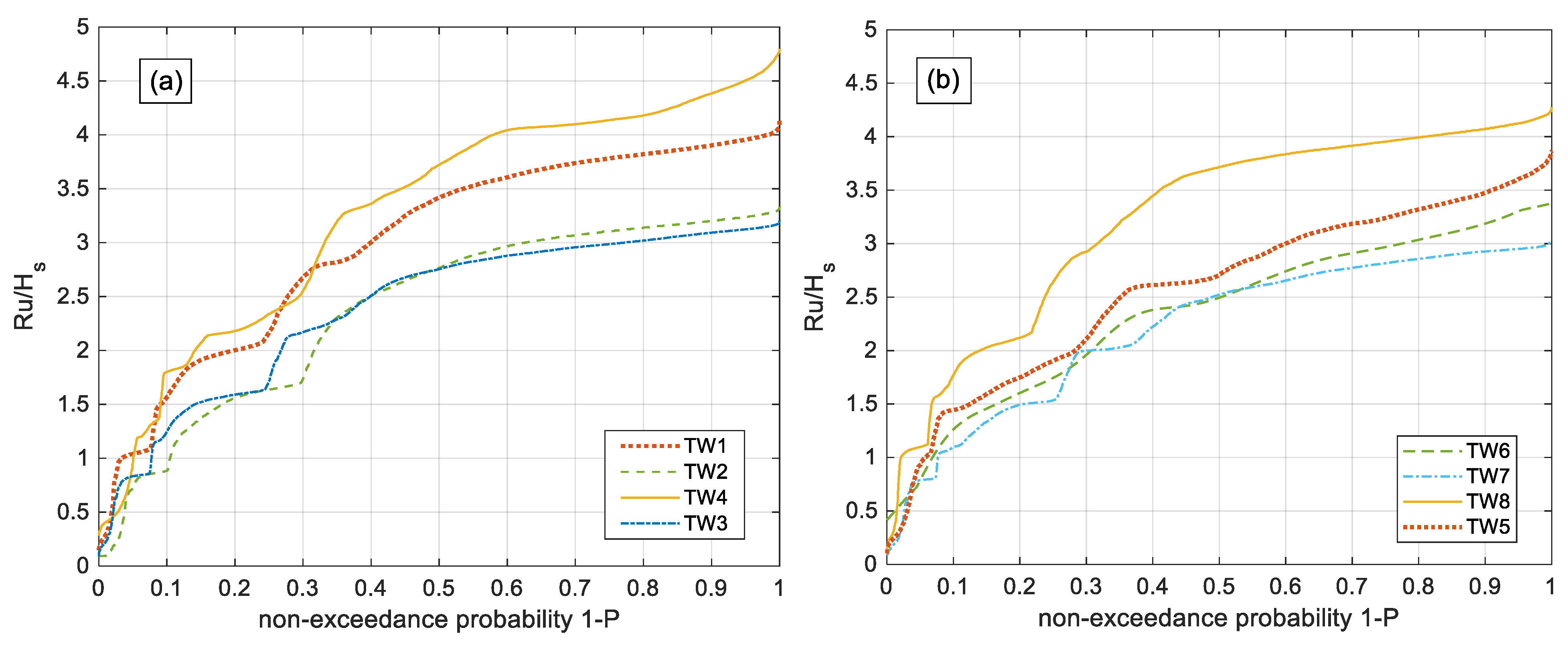
5.1. Probability of Exceedance of the Wave Runup

To statistically characterize the wave runup Ru in time and investigate the effects and the influence of the different tested geometries (slope, berm level, presence of the parapet, wall height) on it, the values of the probability of exceedance of the wave runup (P) were calculated for each test. The curves of probability of non-exceedance (1 − P) of Ru obtained for each test were therefore derived and are reported in Figure 10a,b, for the slopes c4 and c2, respectively. To avoid scale effects, the dimensionless Ru/H_s were used in these Figures.

Overall, the tests with slope c4, characterized by spilling breaker types, tend to give higher Ru-values with respect to the tests with the slope c2 characterized by plunging waves, with maximum values of Ru/H_s in the ranges 3.30–4.75 and 3.00–4.25, respectively.

In both the graphs of Figure 10, the higher curves relate to the tests with parapet TW4 and TW8 (yellow continuous lines), meaning that higher Ru-values are more frequently reached for these tests. Therefore, the parapet may increase the Ru heights of ≈11–12% for the same wave attack with respect to the same structural configuration without parapet. This phenomenon is clearly visible in the example of Figure 11, which compares the same wave event up rushing the crown wall and reaching its instantaneous Ru_max for the four tests TW1, TW2, TW3 and TW4 associated to the slope c4. In particular, Figure 11d (test TW4) shows that the deflection of the up-rushing jet induced by the parapet generates not only higher runup levels, but also higher turbulence and higher air entrainment rates, resulting in a more violent impact with respect to the benchmark case TW1 without parapet Figure 11a).

In Figure 10a,b, the lowest curves are associated to the tests TW3 and TW7 (blue dot-dashed lines), representing the configurations with h_b/H_s = −0.5. The differences among these curves and the corresponding benchmark cases of TW1 and TW5 representing the configurations with h_b/H_s = 0 may be used to quantify the effect of the sea level on Ru: the maximum values of Ru/H_s associated to TW1 and TW5 are approximately +20% higher than TW3 and TW7. Varying h_b/H_s from −0.5 to 0 means increasing h from 0.325 m to 0.35 m, i.e., increasing the sea level of +0.025 m, viz ≈ 0.5 m in real scale conditions. Such a scenario represents an intermediate condition with respect to the predictions of the Intergovernmental Panel on Climate Change (IPCC) that estimates a global average sea-level rise ranging from 0.29–1.10 m by 2100 depending on the emissions scenario [3]. Based on the present results, Ru_max may therefore increase up to +20%, for the same wave attack under a scenario of intermediate sea-level rise. This predicted increase is limited to the configurations considered in this work and does not consider the potentially contributing effects of the wave heights which are also expected to increase due to climate change.

Finally, the curves associated to the tests TW2 and TW6 (green, dashed lines) are very close to the curves of the tests with parapet, in both Figure 10a,b, suggesting therefore that the runup is lower for a lower crown wall height (h_w = 0.04 m). Considering that higher wall heights give lower overtopping discharges, this result suggests that, for the same wave attack, a higher wall allows for higher up-rushing jets that are more likely to spray up vertically and turn back, instead of bending over the top of the wall and overtopping it. This different behaviour can be observed in Figure 11a,b, comparing Ru_max associated to the same wave for the tests TW1 and TW2, respectively. In Figure 11a, the wave sprays up vertically, reaching Ru = 0.111 m and then it turns back without overtopping the wall; in Figure 11b, the wave overturns and overtops the wall before reaching its maximum Ru-value of 0.089 m. Therefore, lower Ru-values are not necessarily associated to lower overtopping discharge q as in the case of emerged berms; indeed, as it can be appreciated in Figure 10 (emerged berm configuration, TW3), the presence of an emerged berm causes an earlier wave breaking along the structure slope that dissipates most of the incident wave energy, determining consequently a bore overtopping flow over the berm and modest runup at the wall and overtopping. Such a correlation lower Ru-lower q does not apply for the configuration with h_w = 0.04.

In summary, the parametric analysis conducted on the results of the video analysis presented in Figure 10 leads to the following main outcomes:

• for the same wave attack, increased rates of Ru of c. 11–12% should be expected when a parapet is included on top of wall;
• in an intermediate condition of sea-level rise projection of c. 0.5 m by the end of the 21st century, Ru_max might increase by up to +20% with respect to present conditions;
• runup heights and overtopping rates (beyond the walls), being differently affected by the structural geometrical parameters, are not necessarily correlated, i.e., the two quantities do not necessarily increase contemporarily.

The limits of these results are discussed in the Conclusions chapter.

5.2. Comparison of the Wave Runup Heights with the Literature

In this sub-section, the results of the video analysis are compared with the commonly applied methods available to quantify the wave runup.

The EurOtop manual [30] proposes the following formulae (Equations (4) and (5) in the manual), for the prediction of Ru_2% in the case of “relatively gentle slopes”, i.e., for values of ξ_m−1,0 ≤ 4 (Ru_2%,Eur):

$$\frac{{Ru}_{2\%}}{H_s}=1.65·{\gamma }_b·{\gamma }_f·{\gamma }_{\beta }·{\xi }_{m-1,0},\mathrm{with}\mathrm{a}\mathrm{maximum}\mathrm{of}:$$

(4)

$$\frac{{Ru}_{2\%}}{H_s}=1.0·{\gamma }_{\beta }·{\gamma }_f·\left(4-\frac{1}{\sqrt{{\gamma }_b·{\xi }_{m-1,0}}}\right),$$

(5)

where γ_b is the influence factor accounting for the presence of a berm, γ_β is the influence factor for oblique wave attacks and γ_f is the influence factor for rough slopes. Since the values of ξ_m−1,0 characterizing the tests TW1-TW8 range between 1.41 and 3.72, these formulae were adopted to estimate the Ru_2%,Eur–values associated to each test. For this purpose, γ_f and γ_β were set equal to 1, whereas γ_b was calculated based on EurOtop Eqs. 5.40, 5.41 and 5.42 and resulted in a value of 0.6 for all the tests. The values of H_s and ξ_m−1,0 were set as equal to the measured values in the wave flume. The use of EurOtop Eq. 5.6, conceived for steep to vertical slopes was evaluated as alternative to Equations (1) and (2) to represent the crown wall on top of the berms. However, Equations (1) and (2) were considered to be more appropriate to describe the geometry of the tested configurations.

The comparison between the 8 values of Ru_2%,video and the corresponding Ru_2%,Eur predictions is portrayed in Figure 12a. Based on the values of Ru_2%,Eur calculated from Equations (4) and (5), the relative differences among video and predicted values of Ru_2% were calculated (Ru_2%,video−Ru_2%,Eur)/Ru_2%,video and plotted as functions of ξ_m−1,0 in Figure 12b. In Figure 12a,b, the data are separated into tests with cotα_d = 4 (“c4”, dots) and cotα_d = 2 (“c2”, squares), and the tests characterized by the presence of the parapet (TW4 and TW8) are circled in red.

In both Figure 12a,b, the points are aligned along the bisector line representing Ru_2%,video = Ru_2%,Eur, suggesting that the results of the video analysis align with the predictions from EurOtop. However, a strong effect of the slope, and consequently of the wave breaking, is observed. All the Ru_2%,video-values associated with the tests “c2” are indeed overestimated by Equations (4) and (5), whereas all the tests “c4” are systematically underestimated. For both the group of tests, the higher differences among EurOtop formulae and video are observed for the tests with parapet, TW4 and TW8, as it could have been expected since Equations (4) and (5) do not account for the presence of the parapet. The important role played by ξ_m−1,0 is even more evident from Figure 12b, where the differences (Ru_2%,video − Ru_2%,Eur)/Ru_2%,video increase almost linearly with increasing ξ_m−1,0-values, being ≤0 for spilling waves and ≥0 for plunging waves. This seems to suggest that for the tested configurations—which do not perfectly fit in any of the cases modelled by EurOtop [30]—a stronger effect of the breaker parameter should be accounted for.

The indications of Ning et al. [8] and Carbone et al. [35] for the maximum runup, Ru_max, were also considered. These two contributions indicate that Ru_max can be 2.6 and 2.75 times the maximum wave height H_max at vertical seawalls [8] and on cliffs [35], respectively. The values of Ru_max/H_max obtained with the videos range in the interval 1.51–2.39, with the minimum and the maximum values being associated with the tests TW7 (Ru_max/H_max = 1.51) and TW4 (Ru_max/H_max = 2.39), respectively. These slightly lower values of Ru_max/H_max recorded with respect to the predicted values from EurOtop can be explained by the wave dissipation process determined by the overtopping flow over the berm. Therefore, based on the results of the video analysis, it could be argued that the inclusion of a smooth berm may reduce the Ru_max by an average the 20% and at least 10% with respect to vertical walls or cliffs. These estimations can be compared with the average reduction of 36% found for armoured berms and berm breakwaters [36].

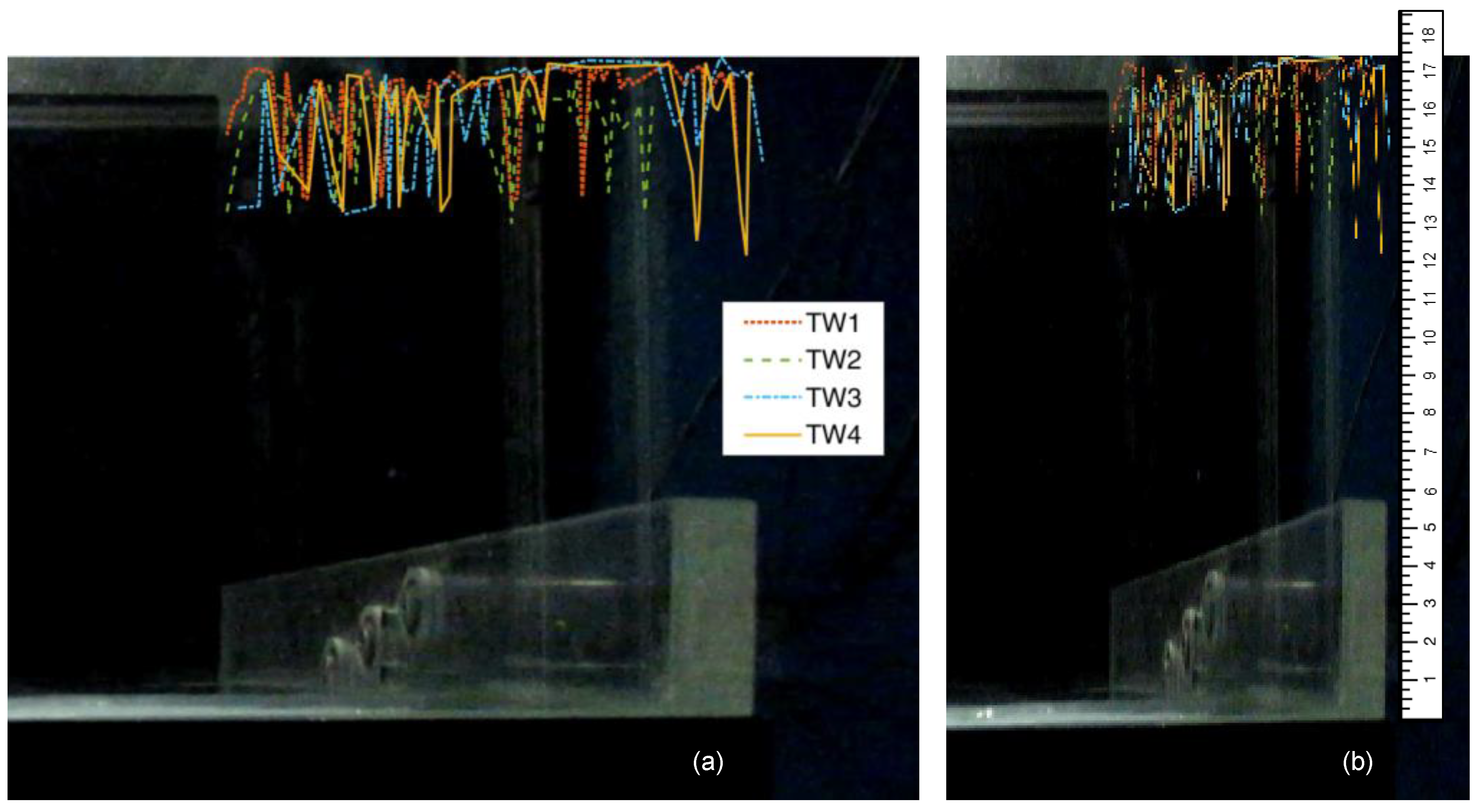
5.3. Wave Runup Envelopes: Design Conditions

Along a 2D, plain slope, the cross-shore position (x) of each instantaneous Ru-value is univocally determined by the Ru-value itself (the higher Ru (z-direction) the farther the horizontal distance covered by the overtopping tongue from the base of the slope, x-direction). Differently, the up rushing along a vertical crown wall generates wave deflection and wave reflection phenomena affecting the linear increasing relationship x-Ru and inducing great variability in the cross-shore spatial distribution of the Ru-values. The presence of 3D, unpredictable effects, which are more pronounced when the parapet is included, induces a spatial variability also along the front-section direction (y).

This sub-section investigates and illustrates the spatial variability of the Ru-values along the x- and y-directions focusing on maxima and minima values, which are useful to get information for design purpose. Section 5.4 will focus on average values to assess ordinary, exercise conditions. To achieve this, for each x-position from x_w,i to x_w,f the corresponding maximum, minimum and mean values of Ru that occurred in that position (if any) were recorded. It was then possible to draw the x-shore envelopes of Ru for each test.

The maximum envelopes of Ru along x are reported in Figure 13 and Figure 14 for the slopes c4 and c2, respectively. In each Figure, both the real images—affected by the perspective distortion (panels a)—and the corrected ones (panels b) are shown. Both images are shown because the distorted pictures show also the variability in the y-direction, whereas the corrected pictures provide the “pure” variability in the x-direction. To assist the interpretation of the results, a ruler marking the vertical heights with respect to the berm crest are included in both the Figures.

The analysis of Figure 13 and Figure 14 leads to the following findings:

• The different configurations associated to the slope c2 (Figure 14) show a higher variability of the Ru-envelopes, ranging between 0.110 and 0.175 m, than the tests c4, which range from between 0.125 and 0.175 m. The effect of the different geometries is indeed more evident in this group of tests with respect to the group c4 (Figure 13); the profile obtained for the test TW6 (lower wall height, h_w = 0.04 m) is well below the profile for the test TW5 (benchmark case for c2) and the profile of TW7 (emerged berm, h_b/H_s = −0.5) is in turn systematically below TW6. Overall, the envelope of TW8 (parapet) is above all the other envelopes, showing Ru-values ranging between 0.140 and 0.175 m;
• Contrary to this and in the case of c4 (Figure 13), the sensitivity to the geometrical parameters is modest and the profiles intersect each other across the whole wall cross section. The envelope of the test with the parapet (TW4) is locally—but not systematically—above all the other envelopes. It is interesting to note that the envelopes associated with TW1 (benchmark case for c4) and to TW4 (emerged berm) show similar variability ranges of Ru (0.133–0.175) and similar spikes;
• A strong variability of Ru across the x- and y-direction is observed. This variability is randomly distributed and the spikes, varying from test to test, are not concentrated either at the front sides of the wall, nor around its middle section. Therefore, it can be concluded that the side walls—which are made of glass—do not generate side effects due to potential friction or capillarity phenomena, and the presence of the pressure transducers located in the middle of the front-section of the walls, do not disturb the runup flow. In conclusion, the variability of the wave runup in the y-direction cannot be explained by side effects from the wave flume side walls.

Based on these results, the recommendation for design purposes is to consider that Ru_max may vary across the wall by approximately ±30% in the case of plunging waves (tests c2) and ±20% in case of spilling waves (tests c4), due to 3D effects. It is notable that only perpendicular waves were tested and therefore the methodology needs also to be applied to wave tank tests to confirm these findings.

5.4. Wave Runup Envelopes: Exercise Conditions

Whilst the upper envelopes represent key data for the design of coastal structures, the mean and the lower envelopes of Ru relate to the typical exercise conditions and provide practical information for the maintenance or upgrade of existing structures to enhance their resilience. Figure 15 compares the upper, mean and lower envelopes of Ru for the tests TW4 and TW8, representing the configurations with parapets characterized by the most severe Ru-values. In the case of TW8 (panel b of Figure 15), it is interesting to see that the lower envelope is frequently and significantly above the wall, revealing that the structure is nearly always overtopped. The mean envelopes of Figure 15 indicate that:

• in average conditions, both the configurations (slopes c4 and c2) are always overtopped;
• in the case of TW4 (spilling breaker type), the average overtopping rate is expected to be modest, since the envelope is very close to the wall top, while in case of TW8 (plunging breaker) the “standard” overtopping represents a severe condition;
• for this latter test, overtopping randomly occurs across the wall front section even in the case of minimum runup: this outcome suggests that the structural configuration corresponding to TW8 is clearly inadequate to face the wave attack conditions in the case of sea-level rise determining h_b = 0.

The average envelopes of the wave runup could also be used to estimate the average overtopping discharge q beyond the wall, by multiplying the average flow depth above the top of the crown wall for the corresponding wave celerity which, under the hypothesis of shallow-water conditions, corresponds approximately to the flow velocity. To complete the estimation of q, the knowledge of the total number of overtopping waves is required to evaluate the time of overtopping, i.e., the portion of the total duration of the tests where overtopping does actually occur. As shown in Figure 3 and specified at the end of Section 3.2, the evaluation of the number of overtopping waves is a matter of ongoing research. The possibility of estimating q from the video analysis of the wave runup would represent an important contribution to the assessment of the hydraulic performance of coastal structures in prototype and field conditions, where the measurement of q is complex and often unfeasible for practical and economic reasons.

6. Conclusions

A statistical and parametric analysis of the wave runup at walls based on the results of video analysis of laboratory experiments of smooth berms with crown walls was presented in this contribution. Such analysis was possible through the implementation of new and innovative procedures of image processing in the framework of an existing methodology of image clustering recently released by the authors. The new procedures were developed to extend the automatic recognition of the free-surface levels from the dike crest (or berm) to the walls area, in order to reconstruct the profiles of the water jets up-rushing along the crown wall and eventually overtopping it. Such procedures were conceived to deal with the complications in the pattern-recognition step represented by the high turbulence and air entrainment rates due to the dynamics of the wave impacts and wave reflection at the walls, by the presence of the wall itself, and by the 3D-perspective distortion effects due to the lens of the camera. Specifically, pre-filtering techniques were applied to exaggerate the contrast of the frames to ease the correct individuation and distinction of the wall from the turbulent flow during the image clustering, while a tool to correct the perspective distortion affecting the walls was included.

The new methodology was applied to the image processing of a subset of eight tests that were specifically selected to analyse the following configurations: two different berm slopes determining spilling and plunging wave-breaking conditions; the case of emerged berms with respect to the still water level, to represent existing defence structures in present exercise conditions, and the case of berms with the crest aligning with the still water level to represent future scenarios of sea-level rise; two wall heights and configurations both including and without a sloping parapet on top of the crown walls installed to reduce the wave overtopping.

The direct outputs of the new methodology of image analysis are the profiles of the free surface along the whole profile of the crown walls of each of the eight selected tests. Based on these profiles, for each time step of each test, the runup height Ru was calculated as the instantaneous maximum elevation reached by the water while up rushing the wall. The records of the Ru-values were further elaborated to perform a statistical analysis of the time and spatial distribution of the wave runup and to investigate how the different tested configurations affect the wave runup itself.

The upper 2% exceedance wave runup values Ru_2%, and the maxima Ru_max, were derived for each test and respectively compared with the methods available from the literature. While following the trend of the EurOtop [30] formulae for the prediction of Ru_2%, the values resulting from the videos show a strong effect of the wave breaking that, if confirmed by further research, might suggest a re-calibration of the literature formula to better represent both spilling and plunging waves. The values of Ru_max/H_max obtained with the videos, ranging in the interval 1.51–2.39, are slightly lower than the predictions of Ning et al. [8] and Carbone et al. [35] for vertical seawalls (2.6) and cliffs (2.75). The dissipation process determined by the presence of the smooth berm before the walls determine therefore a reduction of Ru_max of 20% on average and at least 10%.

Based on the results of the parametric analysis conducted on the probability exceedance curves of the Ru-values reconstructed for each test, it was found that:

• Under an intermediate scenario of sea-level rise of ≈0.5 m up to the end of the 21st century, by assuming the same wave attack conditions, an average increase of ≈20% of Ru_max at the walls could be expected;
• Furthermore, the inclusion of a recurving parapet on top of crown walls as a measure to reduce the wave overtopping discharge might generate an average increase of Ru_max of ≈11–12%, implying higher spray jets, more severe wave loads at the walls and higher wave reflection from the berms.

The analysis of the upper, the mean and the lower envelopes of the Ru-values across the front and the cross section of the walls suggests a significant spatial variability of the runup due to 3D effects. Such variability can be quantified by approximately ±30% in case of plunging waves and of ±20% in case of spilling waves and was observed for all the envelopes, holding therefore for both design conditions (upper envelopes) and exercise conditions (mean envelopes).

The use of the image technique and of the new methodology presented in this contribution can be extremely promising for prototype measurements and assessments and may represent a key information for design purpose. However, it should be noted that all the quantitative outcomes presented in this contribution are the result of small-scale, laboratory experiments and are limited to a specific set of structural configurations. Therefore, the extension to larger scales and a wider range of structures should be supported by further applications of the methodology to prototype and field conditions. Anyway, the whole methodology (new and existing) is completely scale independent and can be directly applied to processing any video record obtained with any camera in any condition (laboratory and field). Therefore, the application of the methodology to new experiments is straightforward.

The main recommendations to apply the proposed methodology to new experiments are related to the use of the camera exclusively, i.e.:

• Well fix the camera and ensure that the framing window is the same for the whole campaign of tests (or at least, for each set of tests);
• Re-calibrate the camera daily and for each set of tests;
• For laboratory tests, if possible, install the camera inside a black box to reduce light reflection and any possible disturbance.

References

1. Reguero, B.G.; Losada, I.J.; Méndez, F.J. A recent increase in global wave power as a consequence of oceanic warming. Nat. Commun. 2019, 10, 205. [Google Scholar] [CrossRef] [Green Version]
2. Timmermans, B.W.; Gommenginger, C.P.; Dodet, G.; Bidlot, J. Global Wave Height Trends and Variability from New Multimission Satellite Altimeter Products, Reanalyses, and Wave Buoys. Geophys. Res. Lett. 2020, 47, e2019GL086880. [Google Scholar] [CrossRef]
3. IPCC. Summary for Policymakers. IPCC Special Report on the Ocean and Cryosphere in a Changing Climate; Pörtner, H.-O., Roberts, D.C., Masson-Delmotte, V., Zhai, P., Tignor, M., Poloczanska, E.K., Eds.; 2019; Available online: https://www.ipcc.ch/srocc/chapter/summary-for-policymakers/ (accessed on 20 May 2023).
4. Priestley, R.K.; Heine, Z.; Milfont, T.L. Public understanding of climate change-related sea-level rise. PLoS ONE 2021, 16, e0254348. [Google Scholar] [CrossRef]
5. Taherkhani, M.; Vitousek, S.; Barnard, P.; Frazer, N.; Anderson, T.; Fletcher, C. Sea-level rise exponentially increases coastal flood frequency. Sci. Rep. 2020, 10, 6466. [Google Scholar] [CrossRef] [Green Version]
6. Nicholls, R.J.; Marinova, N.; Lowe, J.A.; Brown, S.; Vellinga, P.; De Gusmao, D.; Hinkel, J.; Tol, R.S.J. Sea-level rise and its possible impacts given a ‘beyond 4 C. world’ in the twenty-first century. Philos. Trans. R. Soc. A Math. Phys. Eng. Sci. 2011, 369, 161–181. [Google Scholar] [CrossRef] [Green Version]
7. Senechal, N.; Coco, G.; Bryan, K.R.; Holman, R.A. Wave runup during extreme storm conditions. J. Geophys. Res. 2011, 116, C07032. [Google Scholar] [CrossRef] [Green Version]
8. Ning, D.; Wang, R.; Chen, L.; Li, J.; Zang, J.; Cheng, L.; Liu, S. Extreme wave run-up and pressure on a vertical seawall. Appl. Ocean. Res. 2017, 67, 188–200. [Google Scholar] [CrossRef]
9. Melet, A.; Almar, R.; Hemer, M.; Le Cozannet, G.; Meyssignac, B.; Ruggiero, P. Contribution of wave setup to projected coastal sea level changes. J. Geophys. Res. Ocean. 2020, 125, e2020JC016078. [Google Scholar] [CrossRef]
10. Pedersen, J. Wave Forces and Overtopping on Crown Walls of Rubble Mound Breakwaters; Series Paper; Aalborg Universitetsforlag: Aalborg, Denmark, 1996. [Google Scholar]
11. Pearson, J.; Bruce, T.; Allsop, W.; Kortenhaus, A.; Van Der Meer, J.; Smith, J.M. Effectiveness of Recurve Walls in Reducing Wave Overtopping on Seawalls and Breakwaters. In Proceedings of the 29th International Conference on Coastal Engineering, Lisbon, Portugal, 19–24 September 2004; pp. 4404–4416. [Google Scholar]
12. Van Doorslaer, K.; De Rouck, J.; Audenaert, S.; Duquet, V. Crest modifications to reduce wave overtopping of non-breaking waves over a smooth dike slope. Coast. Eng. 2015, 101, 69–88. [Google Scholar] [CrossRef]
13. Molines, J.; Bayon, A.; Gómez-Martín, M.E.; Medina, J.R. Influence of Parapets on Wave Overtopping on Mound Breakwaters with Crown Walls. Sustainability 2019, 11, 7109. [Google Scholar] [CrossRef] [Green Version]
14. Contestabile, P.; Crispino, G.; Russo, S.; Gisonni, C.; Cascetta, F.; Vicinanza, D. Crown Wall Modifications as Response to Wave Overtopping under a Future Sea Level Scenario: An Experimental Parametric Study for an Innovative Composite Seawall. Appl. Sci. 2020, 10, 2227. [Google Scholar] [CrossRef] [Green Version]
15. Molines, J.; Bayón, A.; Gómez-Martín, M.E.; Medina, J.R. Numerical Study of Wave Forces on Crown Walls of Mound Breakwaters with Parapets. J. Mar. Sci. Eng. 2020, 8, 276. [Google Scholar] [CrossRef] [Green Version]
16. Formentin, S.M.; Palma, G.; Zanuttigh, B. Integrated assessment of the hydraulic and structural performance of crown walls on top of smooth berms. Coast. Eng. 2021, 168, 103951. [Google Scholar] [CrossRef]
17. Schüttrumpf, H.; Van Gent, M.R.A. Wave overtopping at seadikes. In Proceedings of the Coastal Structures, Portland, OR, USA, 26–30 August 2003; pp. 431–443. [Google Scholar]
18. Van der Meer, J.; Schrijver, R.; Hardeman, B.; Van Hoven, A.; Verheij, H.; Steendam, G.J. Guidance on Erosion Resistance of Inner Slopes of Dikes from Three Years of Testing with the Wave Overtopping Simulator. Van der Meer Consulting. 2009. Available online: http://resolver.tudelft.nl/uuid:3b4bba65-453c-46f6-b0af-6e6e677cdd77 (accessed on 27 July 2023).
19. Hofland, B.; Diamantidou, E.; van Steeg, P.; Meys, P. Wave runup and wave overtopping measurements using a laser scanner. Coast. Eng. 2015, 106, 20–29. [Google Scholar] [CrossRef]
20. Blenkinsopp, C.E.; Mole, M.A.; Turner, I.L.; Peirson, W.L. Measurements of the timevarying free-surface profile across the swash zone obtained using an industrial LIDAR. Coast. Eng. 2010, 57, 1059–1065. [Google Scholar] [CrossRef]
21. Vousdoukas, M.I.; Kirupakaramoorthy, T.; de la Torre, M.; Wübbold, F.; Wagner, W.; Schimmels, S.; Oumeraci, H. The role of combined laser scanning and video techniques in monitoring wave-by-wave swash zone processes. Coast. Eng. 2014, 83, 150–165. [Google Scholar] [CrossRef]
22. Almeida, L.P.; Masselink, G.; Russell, P.; Davidson, M. Observations of gravel beach dynamics during high energy wave conditions using a laser scanner. Geomorphology 2014, 228, 15–27. [Google Scholar] [CrossRef] [Green Version]
23. Almar, R.; Blenkinsopp, C.; Almeida, L.P.; Cienfuegos, R.; Catalán, P.A. Wave runup video motion detection using the radon transform. Coast. Eng. 2017, 130, 46–51. [Google Scholar] [CrossRef]
24. Holman, R.; Stanley, J. The history and technical capabilities of Argus. Coast. Eng. 2007, 54, 477–491. [Google Scholar] [CrossRef]
25. Archetti, R. Quantifying the evolution of a beach protected by low crested structures using video monitoring. J. Coast. Res. 2009, 25, 884–899. [Google Scholar] [CrossRef]
26. Den Bieman, J.P.; de Ridder, M.P.; van Gent, M.R.A. Deep learning video analysis as measurement technique in physical models. Coast. Eng. 2020, 158, 103689. [Google Scholar] [CrossRef]
27. Addona, F.; Sistilli, F.; Romagnoli, C.; Cantelli, L.; Liserra, T.; Archetti, R. Use of a Raspberry-PiVideo Camera for Coastal Flooding Vulnerability Assessment: The Case of Riccione (Italy). Water 2022, 14, 999. [Google Scholar] [CrossRef]
28. Formentin, S.M.; Gaeta, M.G.; De Vecchis, R.; Guerrero, M.; Zanuttigh, B. Image-clustering analysis of the wave-structure interaction processes under breaking and non-breaking waves. Phys. Fluids 2021, 33, 105121. [Google Scholar] [CrossRef]
29. Formentin, S.M. Key Performance Indicators for the upgrade of existing coastal defense structures. J. Mar. Sci. Eng. 2021, 9, 994. [Google Scholar] [CrossRef]
30. EurOtop. Manual on Wave Overtopping of Sea Defences and Related Structures. An Overtopping Manual Largely Based on European Research, but for Worldwide Application. 2018. Available online: www.overtoppingmanual.com (accessed on 20 July 2023).
31. Gaeta, M.G.; Guerrero, M.; Formentin, S.M.; Palma, G.; Zanuttigh, B. Non-Intrusive Measurements of Wave-Induced Flow over Dikes by Means of a Combined Ultrasound Doppler Velocimetry and Videography. Water 2020, 12, 3053. [Google Scholar] [CrossRef]
32. Duin, R.P.W.; Pekalska, E. Pattern Recognition: Introduction and Terminology; Delft University of Technology: Delft, The Netherlands, 2021; Available online: http://resolver.tudelft.nl/uuid:f5c560ed-5fc7-4320-84b4-a20614012bc7 (accessed on 18 April 2023).
33. Bouguet, J.Y. Camera Calibration Toolbox for Matlab. 2015. Available online: http://www.vision.caltech.edu/bouguetj/calib_doc/index.html (accessed on 1 September 2020).
34. Chan, M. Perspective Control/Correction MATLAB Central File Exchange. 2023. Available online: https://www.mathworks.com/matlabcentral/fileexchange/35531-perspective-control-correction (accessed on 18 April 2023).
35. Carbone, F.; Dutykh, D.; Dudley, J.M.; Dias, F. Extreme wave runup on a vertical cliff. Geophys. Res. Lett. 2013, 40, 3138–3143. [Google Scholar] [CrossRef] [Green Version]
36. Milanian, F.; Zakeri Niri, M.; Najafi-Jilani, A. Effect of hydraulic and structural parameters on Wave Run-Up over Berm breakwaters. Int. J. Nav. Archit. Ocean. Eng. 2017, 9, 282–291. [Google Scholar] [CrossRef] [Green Version]
Figure 1. Schematic layout of the tested cross sections (not in scale) with reference to the symbols and parameters.
Water 15 02729 g001
Figure 2. (a) Cluster map of a frame reproducing a wave overtopping event from the test TW5; (b) profile of the free surface (blue) associated to the overtopping event as obtained from the automatic procedure.
Water 15 02729 g002
Figure 3. Conceptual scheme of the whole methodology of image cluster analysis, where the new part is highlighted in the frame [28,31].
Water 15 02729 g003
Figure 4. Camera framing window, with reference to the positions of the virtual gauges (red) set up to elaborate the outputs of the video cluster analysis. The areas of the window dedicated to the different applications are also indicated. All the measurements are in mm.
Water 15 02729 g004
Figure 5. (a) Example of a frame used for training the cluster model in the new methodology (test TW8); (b) Image as resulting after the application of the new pre-processing techniques; (c) clustered model map of the frame.
Water 15 02729 g005
Figure 6. Example of an instantaneous runup profile (blue) and corresponding maximum runup height (red circle) obtained with the new part of the methodology.
Water 15 02729 g006
Figure 7. Example of the free-surface profile in the runup area before (a) and after (b) the application of the perspective correction.
Water 15 02729 g007
Figure 8. Example of the free-surface profiles in the runup area (blue) and the corresponding instantaneous maximum Ru-values (red circle) obtained for the same test TW8 from two consecutive overtopping events (time instants t = 19.6 s and t = 20.8 s from the beginning of the test for panel (a) and panel (b), respectively). All the measures are in m.
Water 15 02729 g008
Figure 9. Conceptual scheme of the analyses proposed for the wave runup. Now is the number of overtopping events occurring for each test, where “overtopping” refers to the berm.
Water 15 02729 g009
Figure 10. Non-exceedance probability curves (1 − P) of the wave runup for the tests with cot(αd) = 4 (panel (a)) and cot(αd) = 2 (panel (b)).
Water 15 02729 g010
Figure 11. Example of the free-surface profile in the runup area (blue) and the corresponding instantaneous maximum Ru-value (red circle) obtained with the same wave for the tests TW1 (a), TW2 (b), TW3 (c) and TW4 (d).
Water 15 02729 g011
Figure 12. (a) Comparison among the upper 2% Ru-values obtained with the image analysis (Ru2%,video) and estimated with the EurOtop formulae (Ru2%,Eur). (b) Relative difference bewteen the Ru-values ((Ru2%,videoRu2%,Eur)/Ru2%,video) as functions of the Iribarren–Battjes’ breaker parameter ξm−1,0. The red circles indicate the tests with parapets.
Water 15 02729 g012
Figure 13. Upper envelopes of the runup profiles for each of the four tests with cot(αd) = 4. Profiles before (a) and after (b) the application of the perspective correction. The measures in the ruler of panel (b) are in cm.
Water 15 02729 g013
Figure 14. Upper envelopes of the runup profiles for each of the four tests with cot(αd) = 2. Profiles before (a) and after (b) the application of the perspective correction. The measures in the ruler of panel (b) are in cm.
Water 15 02729 g014
Figure 15. Upper, mean and lower envelopes of the runup profiles for the tests with parapet TW4 (panel (a)) and TW8 (panel (b)). The measures in the rulers are in cm.
Water 15 02729 g015