Correction of Fused Rainfall Data Based on Identification and Exclusion of Anomalous Rainfall Station Data

Abstract

High-quality rainfall data are crucial for accurately forecasting flash floods and runoff simulations. However, traditional correction methods often overlook errors in rainfall-monitoring data. We established a screening system to identify anomalous stations using the Hampel method, Grubbs criterion, analysis of surrounding measurement stations, and radar-assisted verification. Three rainfall data-fusion methods were used to fuse rainfall station data with radar quantitative precipitation estimation data; the accuracies of the fused data products with and without anomalous data identification were compared. Validation was performed using four 2012 rainfall events in Hebei Province. The 08:00–19:00 July 3 rainfall event had the highest number of anomalous stations (11.5% of the total), while the 01:00–17:00 August 9 event had the lowest number (7.8%). By comparing stations deemed to be anomalous with stations that were actually anomalous, we determined that the accuracy of reference station determination using Hampel’s method and Grubbs’ test was 94.2%. Radar-assisted validation improved the average accuracy of anomalous station identification during the four typical rainfall events from 89.7 to 93.7%. Excluding anomalous data also significantly impacted the efficacy of rainfall-data fusion, as it improved the quality of the rainfall station data. Among the performance indicators, 95% improved after the exclusion of anomalous data for all four rainfall events.

1. Introduction

Floods occur frequently in China, and have seriously hindered the country’s socioeconomic development [1]. Although floods can have various causes, rainfall is by far the most common and immediate [2]. In the face of increasingly serious flash flood disasters, many countries have developed or are developing effective flash flood monitoring and early warning systems to enhance flood management capabilities, such as the American Hydrological Research Center (HRC) flash flood guidance system (FFGS) [3], which has been widely used in Central America, South Korea and other regions; China’s independent research and development of China Flash Flood Hydrological model (CNFF) [4], which strives to minimize the severity of flash floods. As the most active element of the hydrological cycle, rainfall is the main driver of terrestrial hydrological processes and the most important input for flood forecasting models [5]. However, observation data from a single source contain significant uncertainties due to spatiotemporal variabilities in rainfall [6] and cannot meet the requirements for high-precision and high-resolution rainfall data in the fields of hydrology, agriculture, and ecology. Therefore, accurate spatial estimation of rainfall has been a popular research topic in various fields [7,8].

Since the 1990s, the spatial estimation of rainfall has developed to the multi-source data-fusion stage [9]. This technique involves merging two or more types of rainfall data, producing rainfall products with high precision and high resolution. One widely used method for rainfall-data fusion is Bayesian model averaging (BMA), which was first proposed by Raftery et al. [10] in 2005. Since the output statistics of the model should not be applied to a single set member when the BMA method calibrates the set, which reduces the propagation of the set, Schmeits M J et al. corrected the pre-precipitation probability equation (POP) and additive bias, so that it has become more reliable than traditional methods with these improvements [11]. A newer method for merging rainfall data, the fast Bayesian regression kriging (FBRK) method, was proposed by Yang and Ng in 2019 [12]. Unlike other methods, FBRK merges radar, gauge, and crowdsourced data and analyzes the differences in errors of the various data types, leading to accurate estimations of actual rainfall fields. Additionally, its speed makes it suitable for real-time rainfall estimation [13].

The optimal interpolation (OI) method ensures the accuracy of rainfall data measured at the grid points of monitoring stations and reflects the spatial distribution characteristics of rainfall in remote sensing data. However, its accuracy is affected by the density of the monitoring station network [14]. Presently, kriging with external drift (KED) is the most widely applied and practical method for rainfall-data fusion. In KED, the radar quantitative precipitation estimation (QPE) field is used as auxiliary information to normalize interpolation weights and the spatial correlation between rainfall stations and radar values [15].

Although rainfall-data fusion can be used to obtain accurate and wide-ranging data, it is still affected by the accuracy of the rainfall station data [16,17]. Rainfall monitoring is a critical aspect of hydrological monitoring and is key to the mitigation of rainstorm-induced flooding disasters [18]. However, owing to the poor construction standards of some rainfall stations, it is challenging to maintain stations in mountainous areas. This has made it difficult to ensure that the data produced by these stations are of high quality. Consequently, some rainfall stations produce anomalous data (e.g., overestimates, underestimates, and missing measurements) [19]. Moreover, the topographic conditions of small watersheds in hilly areas are complex and changeable, which has a great impact on the prediction results of hydrological models [20]. Furthermore, owing to the extreme randomity of these anomalies, it is impractical to completely exclude certain stations for rainfall analysis. To ensure that the data from all rainfall stations can be utilized effectively, it is necessary to identify the stations that produced accurate rainfall data in each period, and to exclude the stations with data quality problems [21]. Pegram G used a covariance biplot to screen for outlier sites and an efficient PEM algorithm to repair missing data by combining with singular value decomposition, which was experimentally found to be effective in identifying outliers and repairing missing data [22]. Arumugam P found an effective way of excluding outliers from the rainfall data by using the residuals from the fitted SARIMA model to find outliers and distinguish them from other events [23]. Chao Zhao introduced a robust skewed box plot to remove outliers from skewed data and found that it was possible to robustly identify rainfall outliers as well as retain outliers incorrectly identified by the e standard box plot [24].

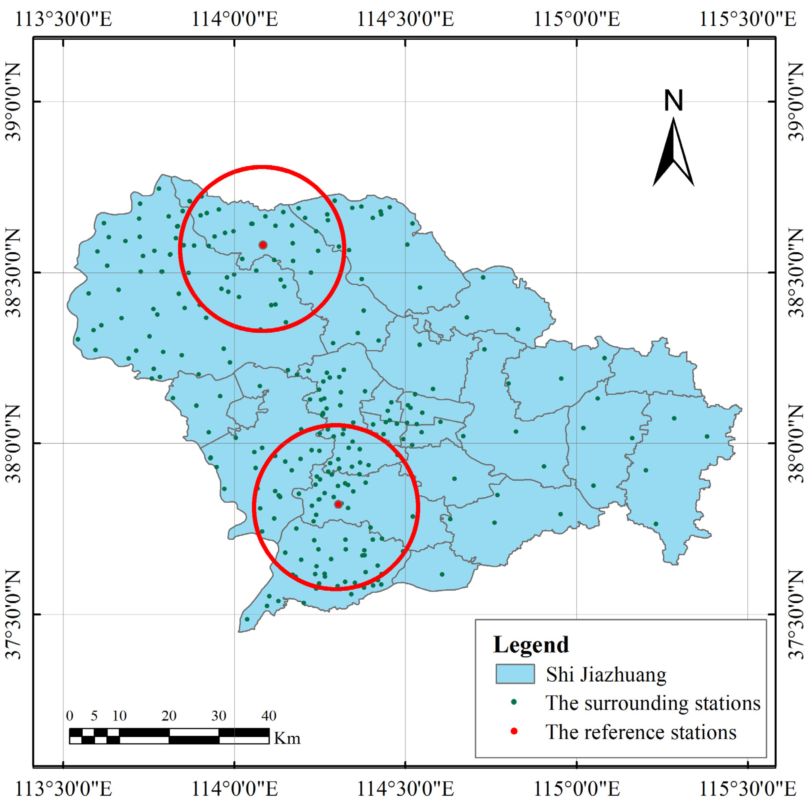
To address the data anomalies caused by poorly maintained rainfall stations in mountainous regions, we developed a three-step method to exclude anomalous stations. First, Hampel’s method and Grubbs’ test were used to screen for stations with anomalous rainfall data, and to select “reference” stations with stable, high-quality rainfall data. Next, adjacent-station comparisons and radar-assisted validation were used to identify anomalous stations, which were subsequently excluded to improve the quality of the rainfall station data. Finally, KED, OI, and an interpolation method based on distance and radar rainfall station data were used to fuse radar QPE data with rainfall station data (for the purposes of this study, this was performed before and after the anomalous stations were excluded). The effects of our anomaly identification method on rainfall-data fusion were analyzed using leave-one-out cross-validation (LOOCV).

2. Study Area and Data

As the prevention and control of flash floods have always been important for China, the provincial government of Hebei has implemented various measures to improve their ability to prevent and mitigate such disasters. However, as shown in the Figure 1, the flash-flood monitoring and warning systems of Hebei are still affected by inaccurate rainfall station data, including overestimates, underestimates, and missing measurements. Moreover, there is currently no effective method for identifying anomalous rainfall stations. As rainfall in Hebei Province is mostly concentrated in July and August, flash floods occur most frequently during this period [25] and have significantly hindered the province’s socioeconomic development. Therefore, we chose to study the rainfall time-series data of Hebei during the July–August 2012 period. Four typical rainfall events were selected for analysis: (i) 08:00–19:00 July 3, (ii) 15:00 July 5 to 11:00 July 6, (iii) 14:00 July 27 to 08:00 July 28 and (iv) 01:00–17:00 August 9.

3. Research Methods

3.1. Method for Anomalous Station Identification

This study proposes a three-step method for the detection and exclusion of anomalous stations. These steps are:

• Selection of reference stations and exclusion of obviously anomalous stations. During this step, Hampel’s method and an improved Grubbs’ test were used to identify anomalous stations.
• The surrounding stations’ analyses, where hourly rainfall data of a station were compared to that of an adjacent reference station to ascertain whether the data were anomalous.
• Radar-assisted validation, to validate the selection of anomalous stations.

3.1.1. Reference Station Determination

• Hampel’s method

Hampel’s method was used to identify outliers. Its basic principle is to assume a distribution and probability model for a given data set and use a consistency test to process the data series according to said assumption [26]. The method to identify anomalies in the rainfall data of each station is as follows:

$$Z_i=\frac{X_i-\left|Median\right|}{\left(\frac{MAD}{0.6745}\right)},$$

(1)

where X_i is a value in the data series X; Median is the median of X; MAD (median absolute deviation) is the median of the data set Y; X = {x₁, x₂, …, x_n} is the rainfall-data sequence of the measurement station; and Y = {y₁, y₂, …, y_n} = {x₁-median, x₂-median, …, x_n-median}. When the value of Z_i (i = 1, 2, …, n) is >2.24, X_i is determined to be an anomalous station and i is the anomalous time of that station.

ii.

Grubbs’ test

After the preliminary identification of anomalous stations, a specific area surrounding each station was demarcated. The area is delimited with a radius of 20 km, and there are about 50 test stations in the area, which are shown in Shijiazhuang as an example (Figure 2). The rainfall values of all stations within that area were used to form a sample sequence, X = (x₁, x₂, …, x_n), which was sorted in ascending order. The value G₀ for the critical coefficient G_{(a, n)} was obtained from the critical value table (

Table 1. The critical value table.

a	n
	3	4	5	6	7	8	9	10	11	12	13	14	15
0.05	1.15	1.45	1.67	1.82	1.94	2.03	2.11	2.18	2.28	2.29	2.33	2.37	2.41
0.025	1.15	1.48	1.71	1.89	2.02	2.13	2.21	2.29	2.36	2.41	2.46	2.51	2.55
0.01	1.15	1.49	1.75	1.94	2.10	2.22	2.32	2.41	2.48	2.55	2.61	2.66	2.71

). The significance level was denoted by a and its value was adopted as 0.05 in this study. Next, G₁ and G_n were calculated as follows:

G₁ = (X_m − x₁)/σ,

(2)

G_n = (x_n − X_m)/σ,

(3)

where n is the number of stations, X_m is the median of the sample, and σ is the standard deviation. G₁ and G_n are statistical quantities.

If G₁ ≥ G_n and G₁ > G₀, x₁ is determined to be an outlier and is rejected; if G_n ≥ G₁ and G_n > G₀, x_n is an outlier and is rejected; if G₁ < G₀ and G_n < G₀, then there is no outlier. If there is an outlier, it is removed and recalculated using the rainfall values of the remaining stations, and the above steps are repeated until there is no outlier.

Using the Grubbs’ test to identify suspected anomalous stations and properly segregating the areas for determination allows for the elimination of confirmed anomalous stations and reduces the impact of outliers on the final results. Additionally, this method saves processing time.

3.1.2. The Surrounding Stations’ Analysis

In this step, rainfall recorded at the same time by a candidate station and reference station were compared. If the candidate station was far away from the reference station, a nearby non-reference station that had been validated as being “normal” (non-anomalous) via comparison with the reference station was used for the comparison. In other words, a candidate station is adjudged as being normal or anomalous through comparisons with adjacent reference stations in terms of average rainfall. This comparison was conducted for different lengths of time: 1, 3, 6, 12, and 24 h. As

Table 2. Rainfall grades.

Grade	Rainfall Amount (mm)
	1 h	3 h	6 h	12 h	24 h
Light rain	0.1–1.5	0.1–2.9	0.1–3.9	0.1–4.9	0.1–9.9
Moderate rain	1.6–6.9	3.0–9.9	4.0–12.9	5.0–14.9	10.0–24.9
Heavy rain	7.0–14.9	10.0–19.9	13.0–24.9	15.0–29.9	25.0–49.9
Rainstorm	15.0–39.9	20.0–49.9	25.0–59.9	30.0–69.9	50.0–99.9
Heavy rainstorm	40.0–49.9	50.0–69.9	60.0–119.9	70.0–139.9	100.0–249.9
Torrential rainstorm	≥50.0	≥70.0	≥120.0	≥140.0	≥250.0

shown, if the difference in average rainfall exceeded one order of magnitude, the candidate station was deemed to be anomalous.

3.1.3. Radar-Assisted Validation

Radar-assisted verification involves using radar data to confirm the screening results of the previous two methods. The method uses the following steps:

• The standard for verifying the determination results of a station was rainfall that occurred when the low-elevation reflectivity of the radar exceeded the 20 dBZ threshold. This means that if the radar detected rainfall at a certain station, it would verify the determination results of that station.
• The rainfall amount recorded at the station was compared with the radar-estimated rainfall intensity. If the station’s rainfall amount was significantly different from the radar-estimated amount, then it was considered anomalous.
• For a station located at the boundaries of a rainfall–non-rainfall area or a rainfall area with large variations in rainfall intensities, the determination results were verified using the spatial reflectivity gradient. This involves examining the changes in reflectivity over a certain distance and determining whether the station’s rainfall amount was consistent with the observed reflectivity changes.

3.2. Methods for Rainfall-Data Fusion

3.2.1. OI

OI transforms discrete rainfall data into an evenly distributed grid of analytical values. The analytical value for each grid point is given by the following equation:

$$R_i^a=R_i^r+{\displaystyle {\sum }_{k=1}^n}{P}_k\left(R_k^g{-R}_k^r\right),$$

(4)

where i is the ordinal number of the grid point; R_i is the rainfall intensity; a, r, and g are the analytical value, initial radar-estimated value, and rain gauge-observed value, respectively; n and k are the number of rain gauges and the station’s ordinal number, respectively; and P_k is the weight factor.

The optimal weight factor is given by:

$${\displaystyle {\sum }_j^N}{P}_j{\mu }_{ij}+{\mathsf{\eta }}_i{P}_j={\mu }_{ki}$$

(5)

where μ_ij is the correlation function between two points i and j, and η_i is the relative mean square error (RMSE) of the observed value at the ith gauge (the actual calculated value is usually 0).

Depending on the density of the station network, the correlation function of the element field usually follows one of two types:

$${\mu }_{ij}=\mathrm{e}\mathrm{x}\mathrm{p}\left(\frac{-r_{ij}}{a}\right),$$

(6)

$${\mu }_{ij}=\mathrm{e}\mathrm{x}\mathrm{p}\left(\frac{-{r_{ij}}^2}{a}\right),$$

(7)

where a is a variable parameter with an appropriate value set according to the network density and r_ij is the distance between i and j.

3.2.2. KED

KED, an extension of Kriging interpolation, interpolates variables as the sum of random and deterministic terms. In our method, KED is performed with the assumption of a linear correlation between the expectation value of the rainfall station data $G\left(x\right)$ and the estimate from radar QPE, $R\left(x\right)$ [27]:

$$G\left(x\right)=a+b\cdot R\left(x\right),$$

(8)

where $G\left(x\right)$ is the rainfall measured by the station at location x; $R\left(x\right)$ is the radar-estimated rainfall at location x; and a and b are pre-determined linear coefficients.

The rainfall at location x₀ is calculated by a linear estimator, whose weights are given by:

$${\displaystyle {\sum }_{i=1}^n}{\lambda }_i^{KED}=1,$$

(9)

$${\displaystyle {\sum }_{i=1}^n}{\lambda }_i^{KED}{R(x}_i)={R(x}_0).$$

(10)

where ${\lambda }_i^{KED}$ is the weight factor; ${R(x}_0)$ is the rainfall at the point to be estimated; ${R(x}_i)$ is the radar-estimated rainfall amount at location x_i.

As trans-Gaussian KED can correlate each given probability quantile to the corresponding quantile of the standard normal probability distribution, it was chosen to transform the data into a strictly continuous cumulative distribution [28].

3.2.3. Distance-Weighted Spatial Interpolation Using Coupled Radar–Gauge Rainfall Data

A method for merging rainfall data suitable for hilly areas (hereinafter called the false alarm ratio (FAR)) was selected for this study. The original dataset for this method includes both radar and gauge data. The radar data (A) are utilized as the primary data to determine the nearest gauge station (B) for each radar station. The monitoring data of the corresponding gauge station are then employed to interpolate the radar station data using the following equation:

$$A_0=\frac{A_1}{B_1}\times B_0,$$

(11)

where $A_0$ is the interpolated rainfall amount of the interpolation point; $A_1$ is the rainfall amount of the gauge station located nearest to the interpolation point; $B_0$ is the radar monitoring value of the interpolation point; and $B_1$ is the radar monitoring value of the nearest gauge station.

3.2.4. LOOCV-Based Evaluation of Rainfall Data-Fusion Methods’ Performances

The performance evaluation of different methods for merging rainfall data was conducted using LOOCV. For each gauge and correction method, their performance was evaluated hourly. The following indicators were used to quantitatively analyze the hourly comparison results of the various merged radar–gauge products and the rainfall monitoring data:

• BIAS: difference between an individual measured value and the average measured value, which is used to determine the precision of the measured results.

  $$\mathrm{B}\mathrm{I}\mathrm{A}\mathrm{S}=\frac{1}{n}{\displaystyle {\sum }_{i=1}^n}\left(R_i-{\widehat{R}}_i\right).$$

  (12)
• RMSE: square root of the deviation between the predicted and ground-truth values. In this study, the ground-truth values were the rainfall values that were obtained after the anomalous data were excluded.

  $$\mathrm{R}\mathrm{M}\mathrm{S}\mathrm{E}=\sqrt{\frac{1}{n}{\displaystyle {\sum }_{i=1}^n}{\left(R_i-{\widehat{R}}_i\right)}^2}.$$

  (13)
• MRTE: mean root transformation error. If the assigned weights are small, MRTE can decrease the principal error associated with high rainfall values.

  $$\mathrm{M}\mathrm{R}\mathrm{T}\mathrm{E}=\frac{1}{n}{\displaystyle {\sum }_{i=1}^n}{\left(\sqrt{R_i}-\sqrt{{\widehat{R}}_i}\right)}^2,$$

  (14)

  where $R_i$ is the observed amount of rainfall at a rainfall station, n is the number of rainfall stations, and ${\widehat{R}}_i$ is the estimated rainfall after data fusion. BIAS ranges from −∞ to +∞; RMSE and MRTE range from 0 to +∞. The optimal value for all three indicators is 0.

4. Results

4.1. Effects of Anomaly Identification and Exclusion

When Hampel’s method and the Grubbs’ test were used to identify anomalous stations during four typical rainfall events, it was found that the 08:00–19:00 July 3 event had the highest number of anomalous stations (11.5% of the total). The event from 01:00 to 17:00 on August 9 had the lowest number of anomalous stations (7.8% of the total) (Figure 3). By comparing the number of anomalous stations detected for each rainfall event to the actual anomalous stations, it was found that the accuracy of reference station determination was 94.2% (

Table 3. Number of detected and actual anomalous stations.

Anomalous Stations	08:00–19:00 h, July 3	15:00, July 5–11:00 h, July 6	14:00 h, July 27–08:00 h, July 28	01:00–17:00 h, August 9
Determined	602	530	451	408
Actual	639	566	472	426

). The anomalous stations were comprised of three types: (i) those that reported a cumulative rainfall of 0 (no data); (ii) those with rainfalls much smaller than those of their adjacent stations (underestimation); and (iii) those with rainfalls much greater than those of their adjacent stations (overestimation). An example is shown in Figure 4, which corresponds to the 08:00–19:00 July 3 event.

It was found that eastern, western, and southern Hebei had many anomalous stations, with the most common being underestimation, “no data,” and overestimation, respectively. Northern Hebei only had a small number of anomalous stations, which occasionally reported a cumulative rainfall of zero (“no data” anomaly).

Next, stations that were deemed anomalous at 08:00 and 17:00 during each rainfall event were manually checked; the accuracy of anomaly detection was >90% in most cases (

Table 4. Accuracy of anomaly detection (%).

Rainfall Event/Time	08:00–19:00 July 3	15:00 July 5–11:00 July 6	14:00 July 27–08:00 July 28	01:00–17:00 August 9
08:00	87	91	88	90
17:00	92	96	92	91

).

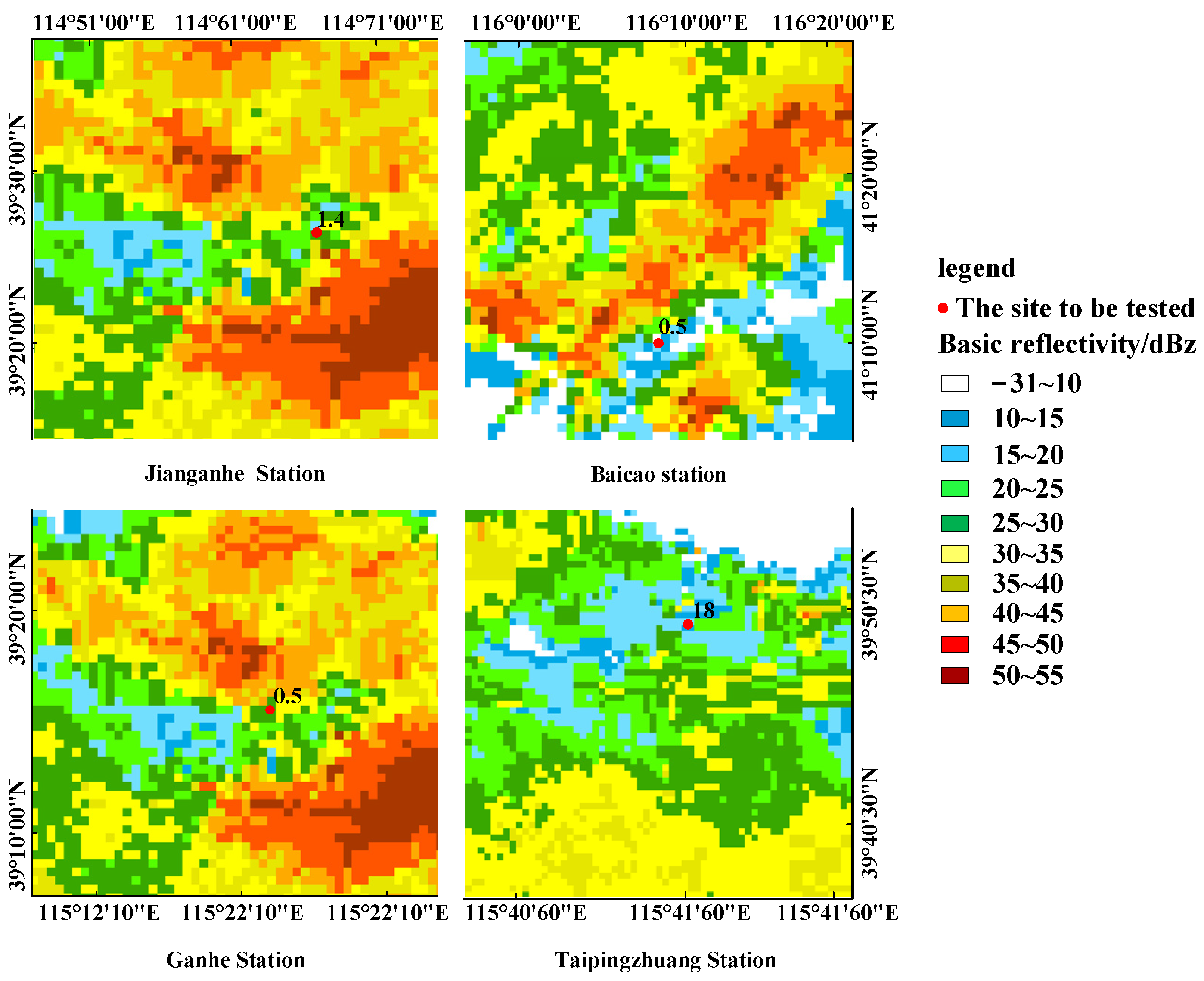
Radar-assisted validation was performed on the anomalous stations that were detected by reference station determination and adjacent-station analysis. Four stations deemed to be anomalous (Baicao, Jianganhe, Ganhe, and Taipingzhuang) at 17:00 on 3 July 2012, were selected for manual validation, which was performed by superimposing the rain gauge-derived rainfall map onto a radar-echo map. Although the four stations were previously determined to be anomalous, it was discovered that the cumulative rainfalls of the Baicao, Jianganhe, Ganhe, and Taipingzhuang stations during the 16:00–17:00 period were 0.5, 1.4, 0.5, and 18.0 mm, respectively. Radar reflectivity was measured every 6 min from 16:00 to 17:00, and the average radar reflectivity values at the four stations (Baicao, Jianganhe, Ganhe, and Taipingzhuang) were 15, 23, 28, and 19 dBZ, respectively. By comparing the hourly rainfall and radar reflectivity at each station, it was found that the Jianganhe and Baicao stations were accurate. The Ganhe station underestimated rainfall, whereas the Taipingzhuang station overestimated rainfall.

During the month of July, large areas of Hebei are rainy, and many rainfall stations report rain. Therefore, radar-assisted validation was performed on three rainfall events in July, at 08:00 and 17:00 (Figure 5 and

Table 5. Accuracy of anomalous station identification in Hebei before and after radar-assisted validation.

Time	08:00–19:00 July 3		15:00 July 5–11:00 July 6		14:00 July 27–08:00 July 28
	08:00	17:00	08:00	17:00	08:00	17:00
Accuracy before radar-assisted validation	88	93	87	89	91	90
Accuracy after radar-assisted validation	93	92	96	94	93	94

). The average accuracy rates of anomaly identification before and after radar verification were 89.7 and 93.7%, respectively.

4.2. Performances of Rainfall Data-Fusion Methods

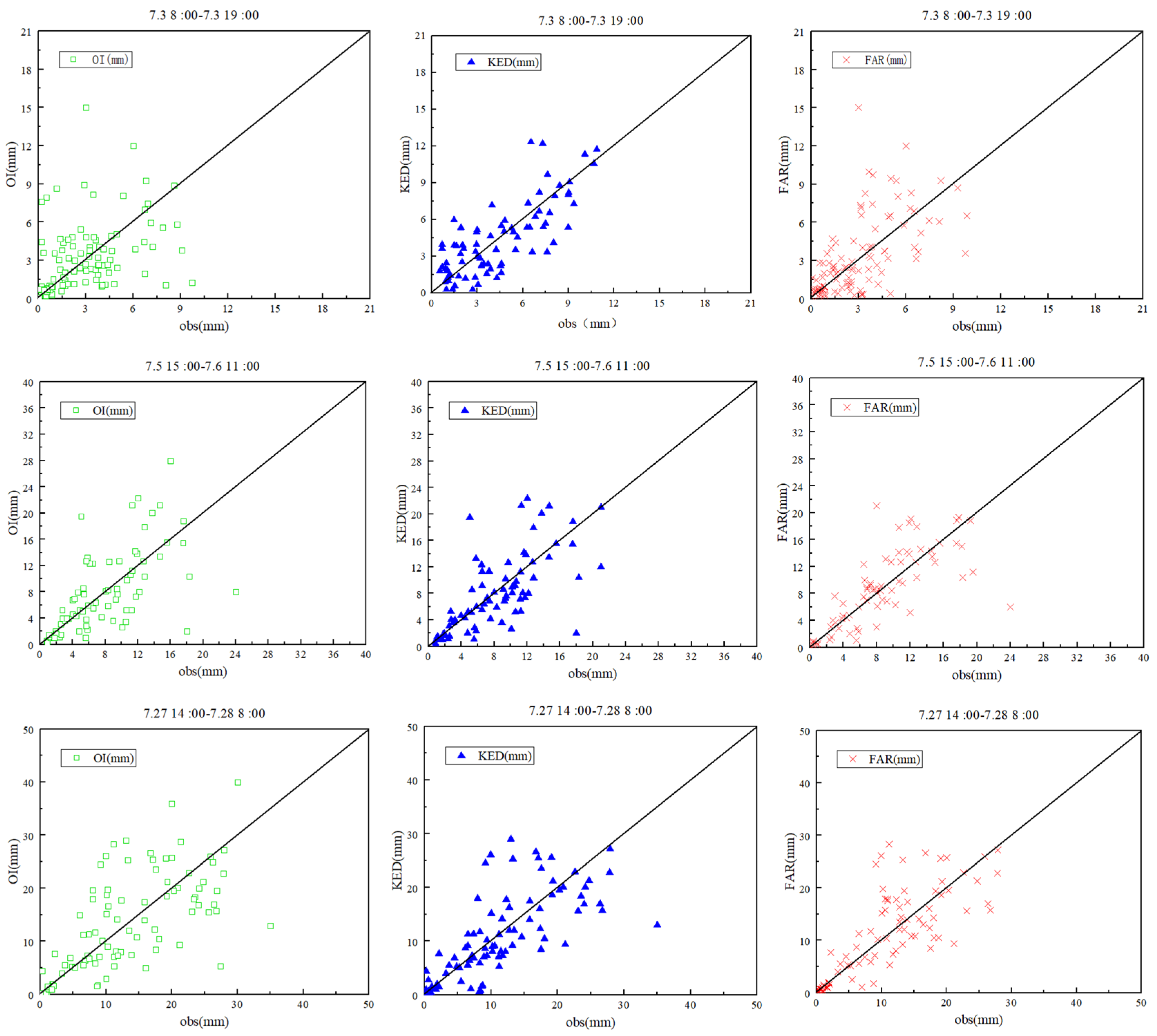
Three data-fusion methods were used to fuse radar QPE and rainfall station data, before and after anomaly detection, which resulted in several fused rainfall products. The performance of each rainfall data-fusion method was evaluated by calculating the BIAS, RMSE, and MRTE of each method for the four typical rainfall events (

Table 6. Performance of each rainfall data-fusion method without the exclusion of anomalous data.

Rainfall Event	Indicator	OI	KED	FAR
08:00–19:00 July 3	BIAS	−0.43	−0.10	−0.16
	RMSE	4.65	2.11	3.16
	MRTE	0.32	0.16	0.16
15:00 July 5–11:00 July 6	BIAS	−0.50	0.16	−0.21
	RMSE	1.86	0.84	1.55
	MRTE	0.49	0.11	0.43
14:00 July 27–08:00 July 28	BIAS	−0.76	0.55	0.69
	RMSE	0.55	0.49	0.47
	MRTE	0.50	0.41	0.53
01:00–17:00 August 9	BIAS	−0.31	−0.36	0.48
	RMSE	1.59	1.01	1.42
	MRTE	0.46	0.33	0.41

). BIAS was analyzed by comparing the fused data products to rainfall station data. It was found that OI had strongly negative BIAS values, while the other methods had BIAS values close to 0. For the 08:00–19:00 event on July 3, all three data-fusion methods exhibited large RMSE values (4.65 (OI), 3.16 (FAR) and 2.11 (KED)), but near-zero values for other indicators.

Figure 6 shows the observed rainfall data plotted against the rainfall estimates derived from the three rainfall data-fusion methods without anomalous station identification.

Next, data fusion was performed using the three different data-fusion methods after anomalous stations were identified and excluded. The performance of each method for the four typical rainfall events is shown in

Table 7. Performance of each rainfall data-fusion method after the exclusion of anomalous data.

Rainfall Event	Indicator	OI	KED	FAR
08:00–19:00 July 3	BIAS	−0.23	−0.08	−0.10
	RMSE	3.32	1.56	2.96
	MRTE	0.16	0.12	0.08
15:00 July 5–11:00 July 6	BIAS	−0.36	0.10	−0.13
	RMSE	1.77	0.86	1.55
	MRTE	0.44	0.06	0.32
14:00 July 27–08:00 July 28	BIAS	−0.77	0.53	0.76
	RMSE	0.52	0.43	0.42
	MRTE	0.50	0.32	0.49
01:00–17:00 August 9	BIAS	−0.23	−0.15	0.33
	RMSE	1.32	0.88	0.85
	MRTE	0.38	0.21	0.42

. By comparing Table 6 and Table 7, it is clear that there are noticeable differences in the quality of the fused rainfall products before and after the exclusion of anomalous stations. We found that 95% of the indicator values showed significant improvement after the exclusion of anomalous rainfall data.

After anomalous station exclusion, for the 08:00–19:00 event on July 3, the BIAS and MRTE values were closer to 0, and RMSE decreased by approximately 1.0. For the 15:00 July 5–11:00 July 6 event, all three indicators decreased by approximately 0.1. The indicators corresponding to the 14:00 July 27–08:00 July 28 event did not change significantly after anomaly identification, which indicates that the removal of anomalies only had a small effect on this set of data. For the 01:00–17:00 August 9 event, the indicator values decreased by 0.2–0.5.

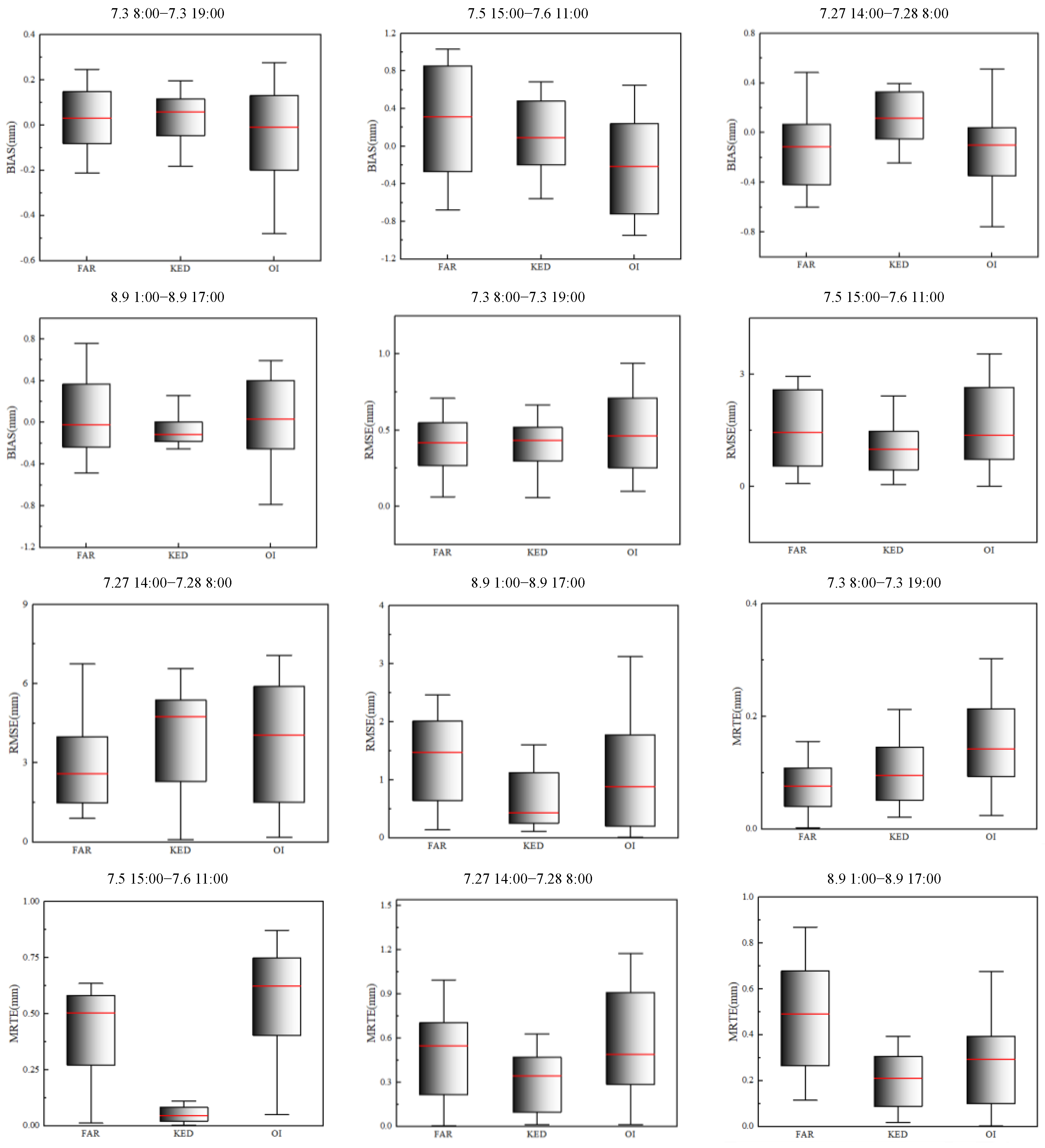
The box plots in Figure 7 depict the values of the performance indicators for the three rainfall data-fusion methods during the four rainfall events. According to the results, KED was the most effective method, followed closely by FAR. The evaluation of the indicators for the four rainfall sessions showed that KED performed slightly better than FAR, while OI was the least effective method. However, FAR performed better than KED for the session 01:00–17:00 h, August 9.

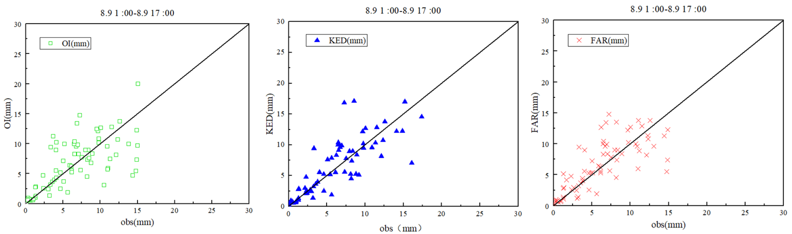
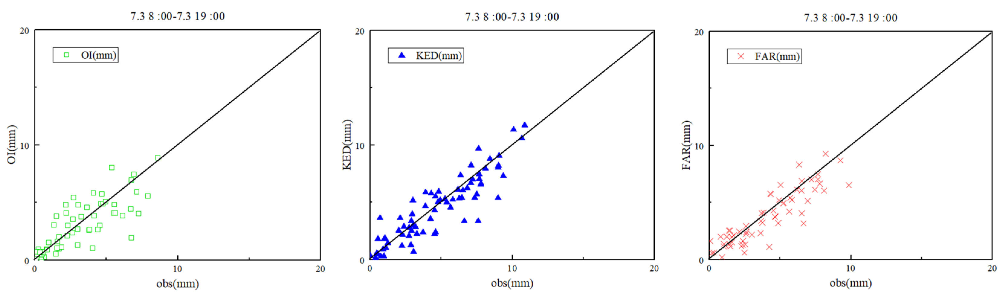
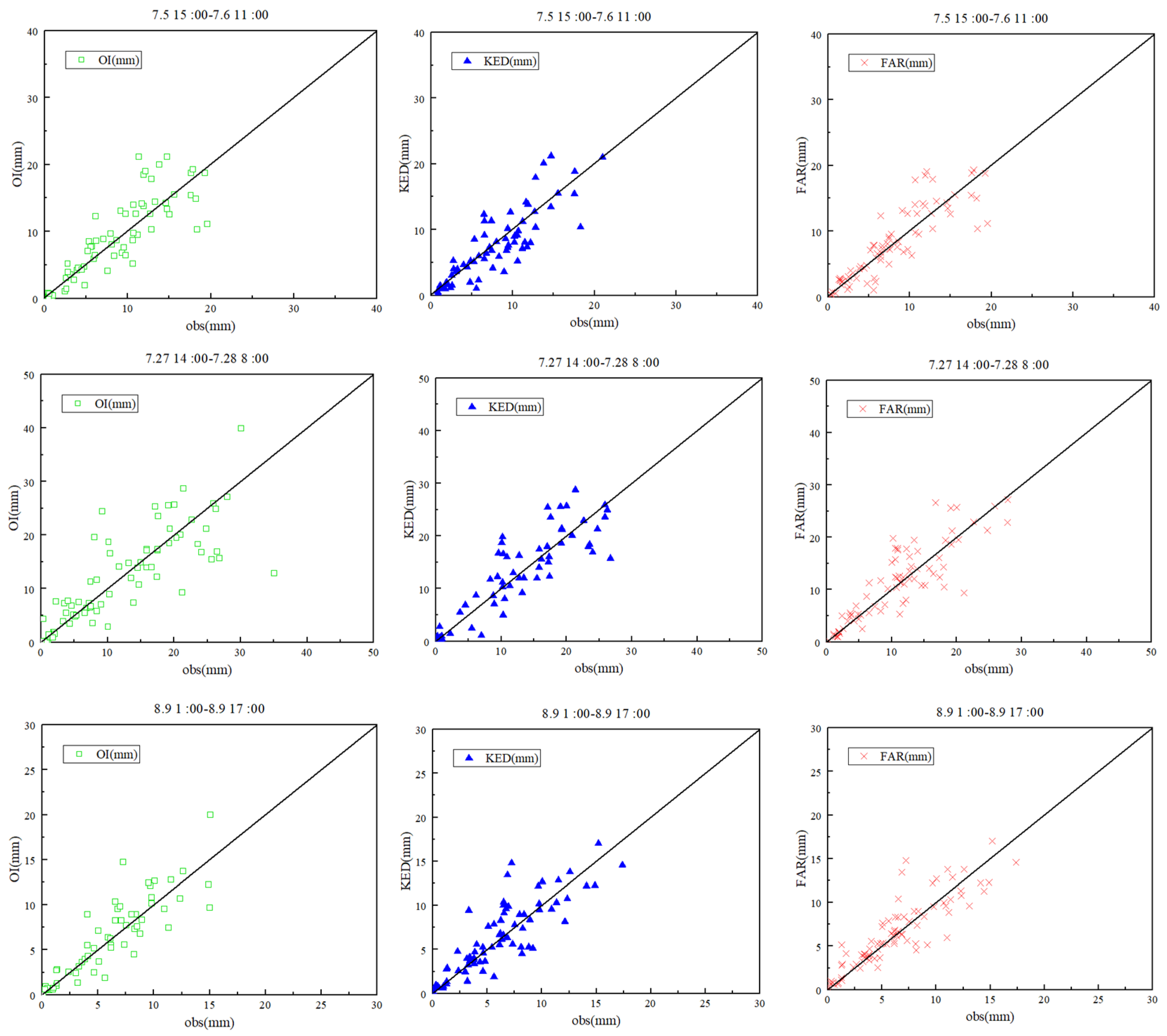
Figure 8 contains scatter diagrams that compare rainfall estimates derived from the three rainfall data-fusion methods plotted against observed rainfall data, after anomalous stations were excluded. As before, OI still had strongly negative BIAS values, while the other methods had average BIAS values close to 0.

By comparing Figure 6 and Figure 8, it is clear that the exclusion of anomalous stations significantly improved the performance of all three rainfall data-fusion methods. This is especially true for the OI and KED methods, as their scatter points became much closer to the 1/1 line after the exclusion of anomalous data. The spreads of the FAR product also became smaller after this step.

5. Discussion

The identification of anomalous rainfall stations in four typical rainfall events using Hampel’s method and Grubbs’ test showed that eastern, western, and southern Hebei have many anomalous stations. This can be attributed to the dense distribution of rainfall stations in those regions. The number of anomalous stations decreased for the later rainfall sessions due to the intensified operation and maintenance of gauge stations after the flood season. However, there was an increase in the number of anomalous stations for the session 01:00–17:00 h, August 9. Manual verification showed that the accuracy rate of the reference station was 94.2%, indicating that the Hampel method and Grubbs criterion had significant effects on the identification of anomalous stations and extreme values. Overall, these methods were helpful in improving the quality of monitoring data [29].

Manual validation performed after the first two steps (reference station determination and adjacent-station analysis) showed that normal stations located at the boundary between rainy and non-rainy areas or areas with significant variations in rainfall intensity were often wrongly classified as anomalous. Hence, the anomalous stations that were detected at 08:00 and 17:00 during three rainfall events in July were selected for radar-assisted validation. The average accuracy of anomaly identification before and after radar-assisted validation were 89.7 and 93.7%, respectively. Hence, radar-assisted validation is suitable for identifying false positives in challenging areas.

The merged rainfall–gauge data were obtained through the application of three different methods before and after the determination of anomalous data. The OI results consistently exhibited strong negative values, regardless of whether the analysis was based on the box diagram or the table of performance indicators, while the average deviations of the other methods were around 0. KED had the best performance, consistent with previous research that shows this method is relatively stable and universal for evaluating most rainfall data merging methods [30,31]. The performance gap between FAR and KED was not large, with FAR occasionally performing better than KED. The excellent performance of FAR was due to its greater suitability for calculating and analyzing the merged rainfall data of hilly regions.

After anomalous stations were excluded, the BIAS and MRTE values of all three data-fusion methods became closer to 0 for the 08:00–19:00 July 3 event; their RMSE values also decreased by approximately 1.0. For the session 15:00 h, July 5–11:00 h, July 6, the results of the three indicators generally decreased by approximately 0.1. There was no significant change in the indicators and anomaly identification for the session 14:00 h, July 27–08:00 h, July 28, and the optimization effect was small. For the session 01:00–17:00 h, August 9, the results of the various indicators generally reduced by 0.2–0.5 compared to those before the identification of anomalous stations. This shows that identifying anomalous stations could eliminate anomalous data and improve the quality of rainfall monitoring data, effectively improving the accuracy of the merged rainfall data. The scatter diagrams used for comparing and analyzing the merged products before and after eliminating anomalous rainfall monitoring data show that the overall correction effects improved significantly after anomaly identification, indicating that the quality of rainfall data at gauge stations determines that of the merged rainfall products [17,32].

6. Conclusions

In this study, we proposed a three-step method for anomalous station identification based on Hampel’s method, adjacent-station analysis, and radar-assisted validation, and used it to detect anomalies in the rainfall station data of Hebei in July–August 2012. In addition, three rainfall data-fusion methods were used to fuse radar QPE data with rainfall station data, before and after anomalous station identification. The results of data fusion with and without anomalous station identification were then compared. The conclusions of this study are as follows:

• By conducting anomalous station identification using Hampel’s method and Grubbs’ test (i.e., “reference station determination”) on four typical rainfall events, it was found that the 08:00–19:00 July 3 event had the highest number of anomalous stations (11.5% of all anomalous stations), while the 01:00–17:00 August 9 event had the smallest number of anomalous stations (7.8% of all anomalous stations). By comparing the anomalous stations that were detected for each rainfall event to the stations that were known to be anomalous, it was determined that the accuracy of reference station determination was 94.2%.
• Radar-assisted validation increased the average accuracy of anomaly identification for the four typical rainfall events from 89.7 to 93.7%. Hence, this method is suitable for identifying false positives in challenging areas (i.e., the boundary between rainy and non-rainy areas, and areas that contain large variations in rainfall intensity).
• By analysing box plots for the performance indicators of each data-fusion method in four rainfall events, KED was found to be the best performing method for rainfall-data fusion. FAR was the second best method, and was only slightly less effective than KED.
• The exclusion of anomalous stations had a pronounced impact on the results of rainfall-data fusion, as it improved the quality of the rainfall station data. We found that 95% of the performance indicators were improved by the exclusion of anomalous data. In scatter diagrams comparing rainfall station data to rainfall estimates derived from fused rainfall products, it was found that the exclusion of anomalous data had the greatest impact on the OI and KED products, with the scatter points much closer to the 1/1 line. In other words, anomalous data exclusion, which improves the quality of rainfall station data, is a very effective way to improve the quality of fused rainfall products.
• A method combining Hampel and Grubbs criterion was used to determine the reference station, by which to identify the surrounding measuring stations. Using radar-assisted inspection, the vast majority of abnormal rainfall data could be eliminated, which greatly improved the quality of rainfall monitoring by rainfall stations. This method obtains high-resolution and high-precision rainfall fusion products by using high-quality data to carry out rainfall fusion. Finally, it will provide strong support for flash flood disaster forecasting and early warning.

References

1. Zhang, J.; Zhou, C.; Xu, K.; Watanabe, M. Flood disaster monitoring and evaluation in China. Glob. Environ. Chang. B 2002, 4, 33–43. [Google Scholar] [CrossRef]
2. Smith, D.D.; Wischmeier, W.H. Rainfall erosion. Adv. Agron. 1962, 14, 109–148. [Google Scholar] [CrossRef]
3. Georgakakos, K.P.; Modrick, T.M.; Shamir, E.; Campbell, R.; Cheng, Z.; Jubach, R.; Sperfslage, J.A.; Spencer, C.R.; Banks, R. The flash flood guidance system implementation worldwide: A successful multidecadal research-to-operations effort. Bull. Am. Meteorol. Soc. 2022, 103, E665–E679. [Google Scholar] [CrossRef]
4. Wang, Y.; Liu, R.; Guo, L.; Tian, J.; Zhang, X.; Ding, L.; Wang, C.; Shang, Y. Forecasting and providing warnings of flash floods for ungauged mountainous areas based on a distributed hydrological model. Water 2017, 9, 776. [Google Scholar] [CrossRef] [Green Version]
5. Ntajal, J.; Lamptey, B.L.; Mahamadou, I.B.; Nyarko, B.K. Flood disaster risk mapping in the lower Mono river basin in Togo, West Africa. Int. J. Disaster Risk Reduct. 2017, 23, 93–103. [Google Scholar] [CrossRef]
6. Wilson, J.W. Integration of radar and raingage data for improved rainfall measurement. J. Appl. Climatol. 1970, 9, 489–497. [Google Scholar] [CrossRef]
7. Hu, Q.; Li, Z.; Wang, L.; Huang, Y.; Wang, Y.; Li, L. Rainfall spatial estimations: A review from spatial interpolation to multi-source data merging. Water 2019, 11, 579. [Google Scholar] [CrossRef] [Green Version]
8. Barrett, E.C.; Beaumont, M.J. Satellite rainfall monitoring: An overview. Remote Sens. Rev. 1994, 11, 23–48. [Google Scholar] [CrossRef]
9. Duan, Z.; Ren, Y.; Liu, X.; Lei, H.; Hua, X.; Shu, X.; Zhou, L. A comprehensive comparison of data fusion approaches to multi-source precipitation observations: A case study in Sichuan Province, China. Environ. Monit. Assess. 2022, 194, 422. [Google Scholar] [CrossRef]
10. Raftery, A.E.; Gneiting, T.; Balabdaoui, F.; Polakowski, M. Using Bayesian model averaging to calibrate forecast ensembles. Mon. Weather Rev. 2005, 133, 1155–1174. [Google Scholar] [CrossRef] [Green Version]
11. Schmeits, M.J.; Kok, K.J. A comparison between raw ensemble output, (modified) Bayesian model averaging, and extended logistic regression using ECMWF ensemble precipitation reforecasts. Mon. Weather Rev. 2010, 138, 4199–4211. [Google Scholar] [CrossRef]
12. Yang, P.; Ng, T.L. Fast Bayesian regression kriging method for real-time merging of radar, rain gauge, and crowdsourced rainfall data. Water Resour. Res. 2019, 55, 3194–3214. [Google Scholar] [CrossRef]
13. Kang, H.B.; Jung, Y.J.; Park, J. Fast Bayesian Functional Regression for Non-Gaussian Spatial Data. Bayesian Anal. 2023, 1, 1–32. [Google Scholar] [CrossRef]
14. Zhang, T.; Li, Y.; Li, J.; Li, Z.; Wang, C.; Liu, J. Quantitative Estimation and Fusion Optimization of Radar Rainfall in Duanzhuang Watershed in the Eastern foot of Taihang Mountains. Authorea 2023. [Google Scholar] [CrossRef]
15. Crane, R.K. Automatic cell detection and tracking. IEEE Trans. Geosci. Electron. 1979, 17, 250–262. [Google Scholar] [CrossRef]
16. Velasco-Forero, C.A.; Sempere-Torres, D.; Cassiraga, E.F.; Jaime Gómez-Hernández, J. A non-parametric automatic blending methodology to estimate rainfall fields from rain gauge and radar data. Adv. Water Resour. 2009, 32, 986–1002. [Google Scholar] [CrossRef]
17. Ochoa-Rodriguez, S.; Wang, L.-P.; Willems, P.; Onof, C. A review of radar-rain gauge data merging methods and their potential for urban hydrological applications. Water Resour. Res. 2019, 55, 6356–6391. [Google Scholar] [CrossRef]
18. de Vos, L.W.; Leijnse, H.; Overeem, A.; Uijlenhoet, R. Quality control for crowdsourced personal weather stations to enable operational rainfall monitoring. Geophys. Res. Lett. 2019, 46, 8820–8829. [Google Scholar] [CrossRef] [Green Version]
19. Sciuto, G.; Bonaccorso, B.; Cancelliere, A.; Rossi, G. Quality control of daily rainfall data with neural networks. J. Hydrol. 2009, 364, 13–22. [Google Scholar] [CrossRef]
20. Guo, B.; Zhang, J.; Xu, T.; Croke, B.; Jakeman, A.; Song, Y.; Yang, Q.; Lei, X.; Liao, W. Applicability assessment and uncertainty analysis of multi-precipitation datasets for the simulation of hydrologic models. Water 2018, 10, 1611. [Google Scholar] [CrossRef] [Green Version]
21. Wang, H.; Zhang, N.; Du, E.; Yan, J.; Han, S.; Li, N.; Li, H.; Liu, Y. An adaptive identification method of abnormal data in wind and solar power stations. Renew. Energy 2023, 208, 76–93. [Google Scholar] [CrossRef]
22. Pegram, G. Patching rain-fall data using regression methods. 3. Grouping, patching and outlier detection. J. Hydrol. 1997, 198, 319–334. [Google Scholar] [CrossRef]
23. Arumugam, P.; Saranya, R. Outlier detection and missing value in sea-sonal ARIMA model using rainfall data. Mater. Today Proc. 2018, 5, 1791–1799. [Google Scholar] [CrossRef]
24. Zhao, C.; Yang, J. A robust skewed boxplot for detecting outliers in rainfall observations in real-time flood forecasting. Adv. Meteorol. 2019, 2019, 1795673. [Google Scholar] [CrossRef] [Green Version]
25. Ma, M.; He, B.; Wan, J.; Jia, P.; Guo, X.; Gao, L.; Maguire, L.W.; Hong, Y. Characterizing the flash flooding risks from 2011 to 2016 over China. Water 2018, 10, 704. [Google Scholar] [CrossRef] [Green Version]
26. Pearson, R.K. Outliers in process modeling and identification. IEEE Trans. Control Syst. Technol. 2002, 10, 55–63. [Google Scholar] [CrossRef]
27. Haberlandt, U. Geostatistical interpolation of hourly precipitation from rain gauges and radar for a large-scale extreme rainfall event. J. Hydrol. 2007, 332, 144–157. [Google Scholar] [CrossRef]
28. Erdin, R.; Frei, C.; Künsch, H.R. Data transformation and uncertainty in geostatistical combination of radar and rain gauges. J. Hydrometeorol. 2012, 13, 1332–1346. [Google Scholar] [CrossRef]
29. Davies, L.; Gather, U. The identification of multiple outliers. J. Am. Stat. Assoc. 1993, 88, 782–792. [Google Scholar] [CrossRef]
30. Qiu, Q.; Liu, J.; Tian, J.; Jiao, Y.; Li, C.; Wang, W.; Yu, F. Evaluation of the radar QPE and rain gauge data merging methods in Northern China. Remote Sens. 2020, 12, 363. [Google Scholar] [CrossRef] [Green Version]
31. Nanding, N.; Rico-Ramirez, M.A.; Han, D. Comparison of different radar-raingauge rainfall merging techniques. J. Hydroinform. 2015, 17, 422–445. [Google Scholar] [CrossRef]
32. Jewell, S.A.; Gaussiat, N. An assessment of kriging-based rain-gauge–radar merging techniques. Q. J. R. Meteorol. Soc. 2015, 141, 2300–2313. [Google Scholar] [CrossRef]
Figure 1. Map of rainfall stations in Hebei Province.
Water 15 02541 g001
Figure 2. Map of Shijiazhuang reference station and distribution of surrounding stations.
Water 15 02541 g002
Figure 3. Number and percentage of anomalous stations during four typical rainfall events.
Water 15 02541 g003
Figure 4. Types of anomalies during the 08:00–19:00 July 3 rainfall event.
Water 15 02541 g004
Figure 5. Validation of anomalous station identification.
Water 15 02541 g005
Figure 6. Scatter diagrams comparing rainfall station data (1/1 line) to rainfall estimates derived from rainfall-data fusion (scatter points), without the exclusion of anomalous data.
Water 15 02541 g006aWater 15 02541 g006b
Figure 7. Box plots of the data-fusion performance indicators for four rainfall events.
Water 15 02541 g007
Figure 8. Scatter diagrams comparing rainfall station data (1/1 line) to rainfall estimates derived from rainfall-data fusion (scatter points) after the exclusion of anomalous data.
Water 15 02541 g008aWater 15 02541 g008b