
Automatic River Planform Recognition Tested on Chilean Rivers

 ,
,
Abstract
:
1. Introduction
2. Methodology
2.1. Ability to Deal with Rivers with Highly Variable AC Width
2.2. Improvement of Some Indicators and Value Functions (VF)
- -
- Adjustments or refinement of Value Functions (definition, attributes, and their parameter values);
- -
- Determination of sinuosity;
- -
- Constrained sinuosity conditions;
- -
- Adoption of multiplicative scalar Value Functions (VFs).
2.3. Introduction of the Holistic Categorical Tool Paired with the Planform Tool
- -
- Identify the discontinuities of Planform type (output of Planform);
- -
- Then, proceed from the upstream toward the downstream while considering each generic slice i.
- -
- It determines the “distance of constancy D(i)”; i.e., the number of slices along which the previous type (now changed) were kept constant within half of the significant length centered in the current slice; this distance, by construction, progressively reduces while moving to slices ahead of a discontinuity.
- -
- “prevailing type K steps forward window”: the algorithm here identifies the most frequent type occurring within the K slices ahead.
- -
- “prevailing type in the D residual forward window “: analogous task, but in a reduced window of just K − D(i) − 1 slices ahead: this is a moving window ahead within a K horizon, the start of which is anchored to the previous discontinuity (it is changed when the algorithm processes the next discontinuity) and that progressively becomes shorter. Its purpose is to consider which value is prevailing in the vicinity in front of the current slice and so avoid it while concluding that a certain type is prevailing in the K window ahead when it indeed is, but leaving “a hole” (i.e., different types are present) in the most proximal slices:
- When the prevailing type in this window is the same than before the (last) discontinuity → current type was a “local hole” and therefore the previous value is maintained instead;
- When it is “not detectable”, it is maintained;
- Otherwise, the prevailing type within the K forward window is adopted.
- -
- It identifies discontinuities in the sequence of types just determined by the Holistic I round;
- -
- Where there is no discontinuity, it maintains the already-computed value;
- -
- Where there is a discontinuity, if the distance D(i) from the last discontinuity is D(i) < K, it adopts the value type occurring upstream of the discontinuity; otherwise, it maintains the current one.
3. Case Study
3.1. Study Area
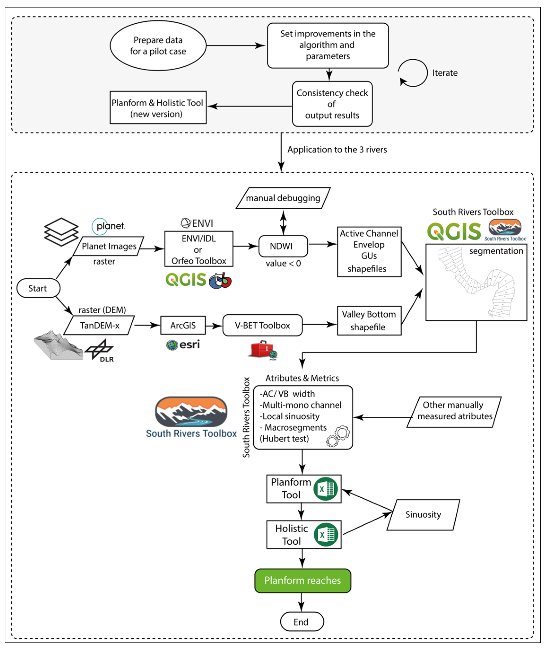
3.2. Data and Methods
- -
- ID of the slice or DGO (i);
- -
- Length of discretization slice (all slices equal; 50 m was adopted for the three rivers);
- -
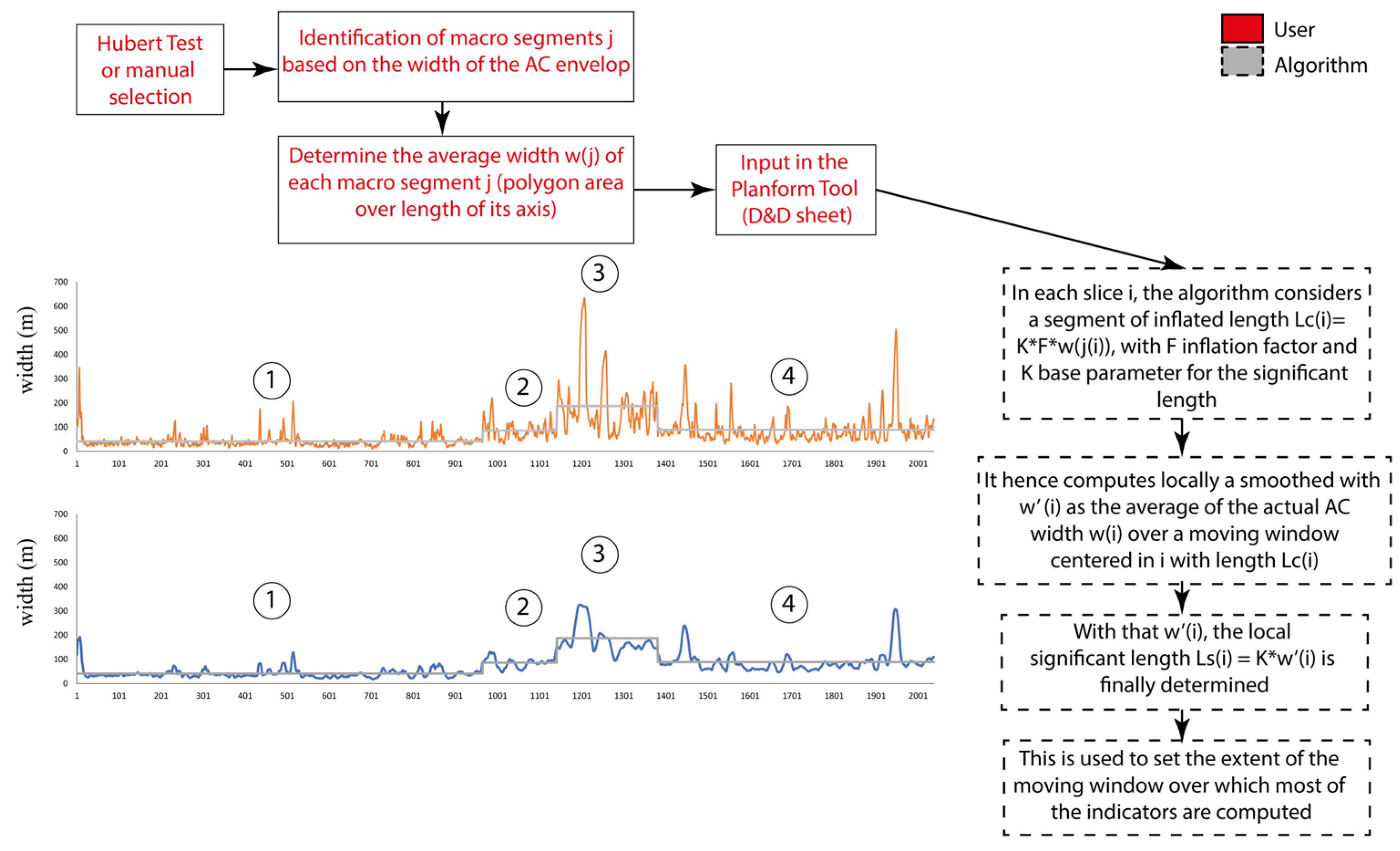
- Length LH(j) of the Hubert segment j(i) corresponding to slice i (several slices were associated with the same segment j); reference moving window length L(i) = f ∗ LH(j(i)), over which the reference width w(j(i)) was calculated, with f inflation factor (f ≥ 1) → corresponding significant length (smoothed) LS(i) = K ∗ w(j(i)) with K characteristic parameter. Notice hence that w(j(i)) in general did not coincide with the local slice width w(i), which could be much more variable along the river: w(j(i)) is a filtered out relative of w(i);
- -
- AC envelope area (or width);
- -
- VB area (or width);
- -
- Area of left, right, and point bank attached bars; area of mid-channel bars;
- -
- Number of active channels;
- -
- Max, min, average width of low-flow water channel;
- -
- Max and average distance between two low-flow channels (when multi-channel);
- -
- Max whole length of water channel crossing slice i (from its departure from main channel until its joining downstream);
- -
- Area of wetlands within the VB (for slice i);
- -
- Sinuosity of reach in which slice i falls (see discussion above on sinuosity iteration).
4. Results and Discussion
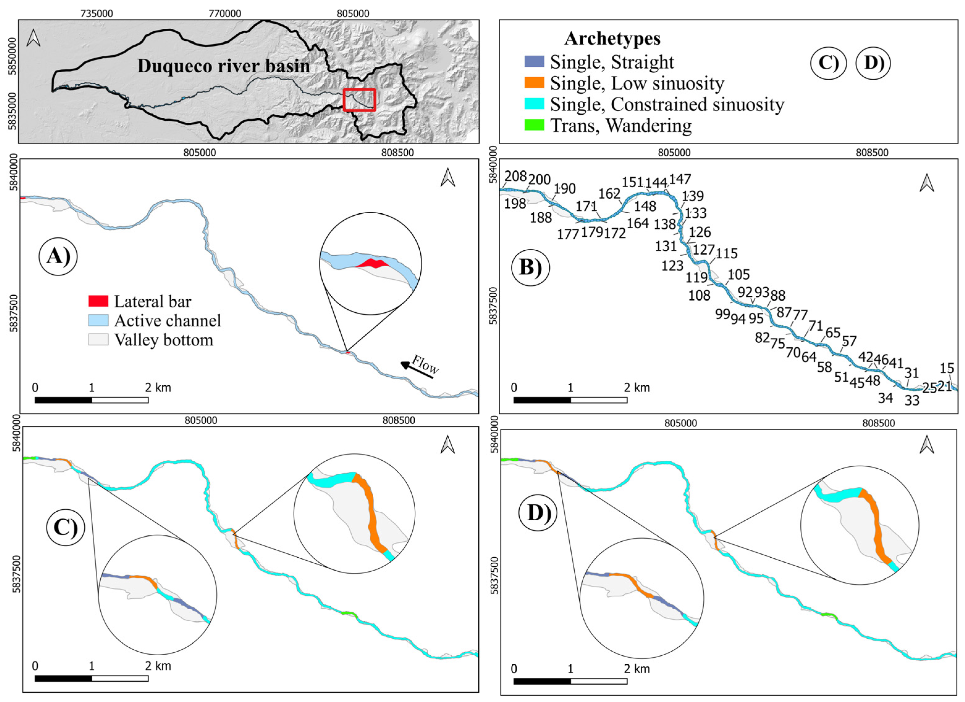
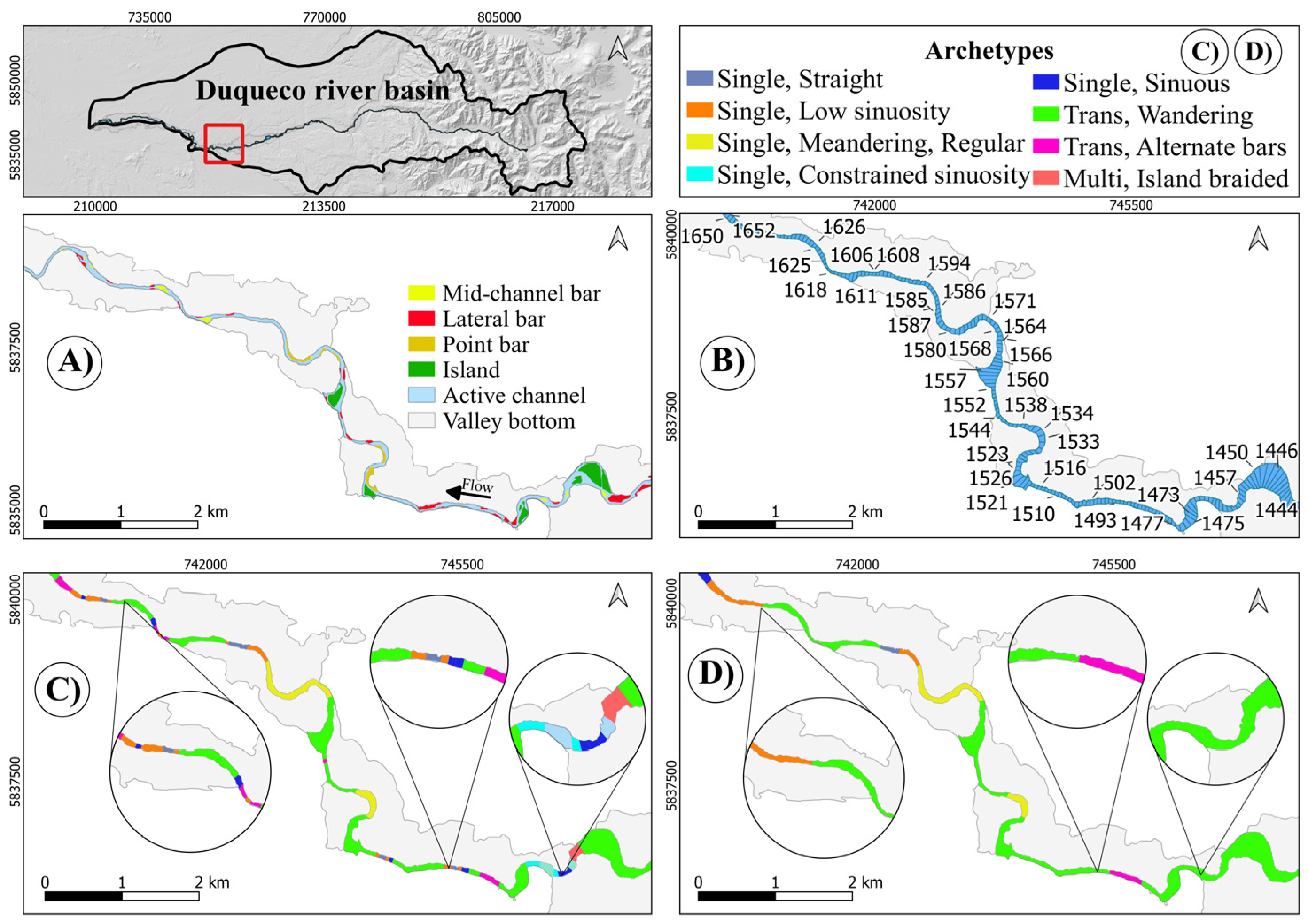
4.1. Duqueco River
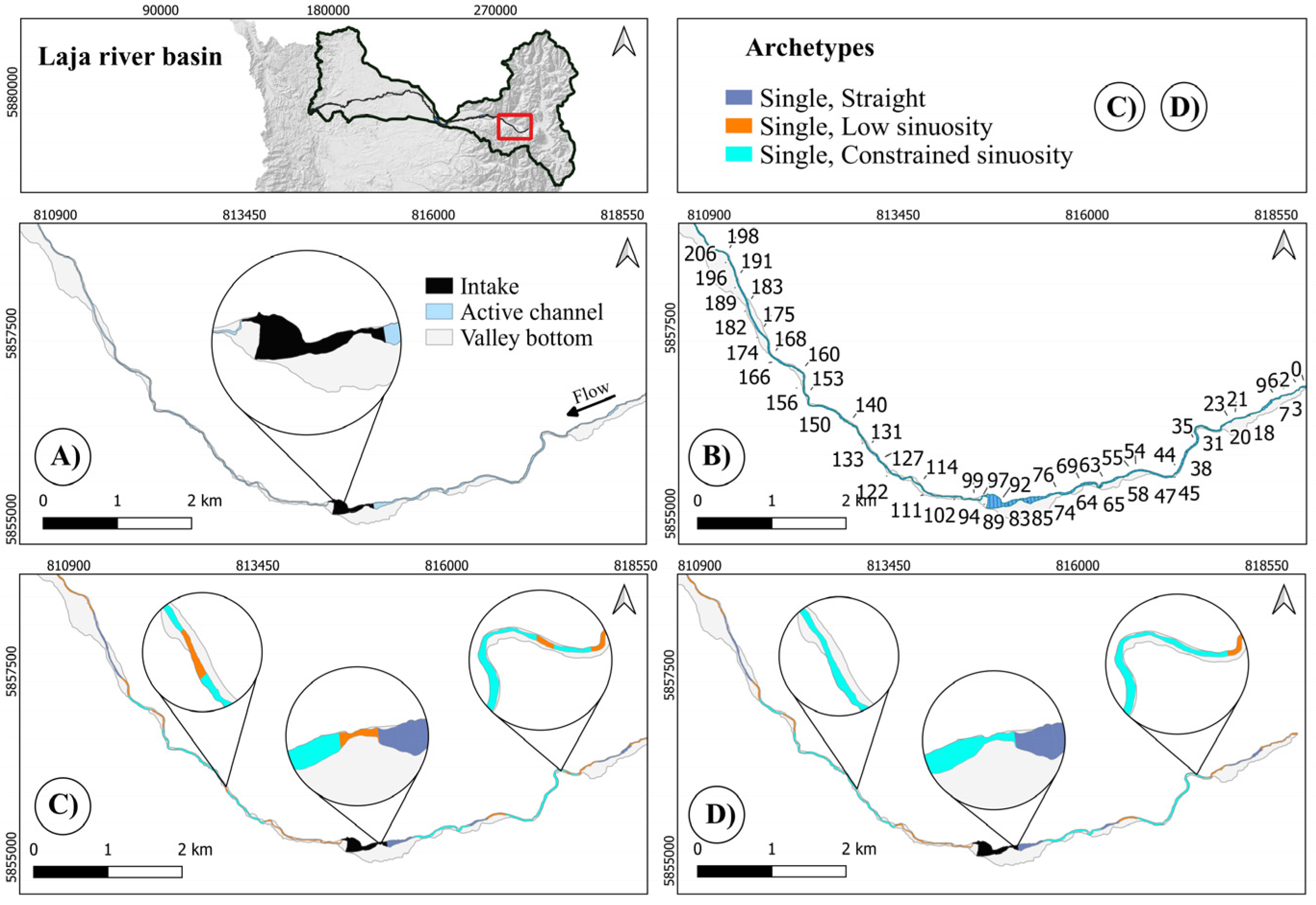
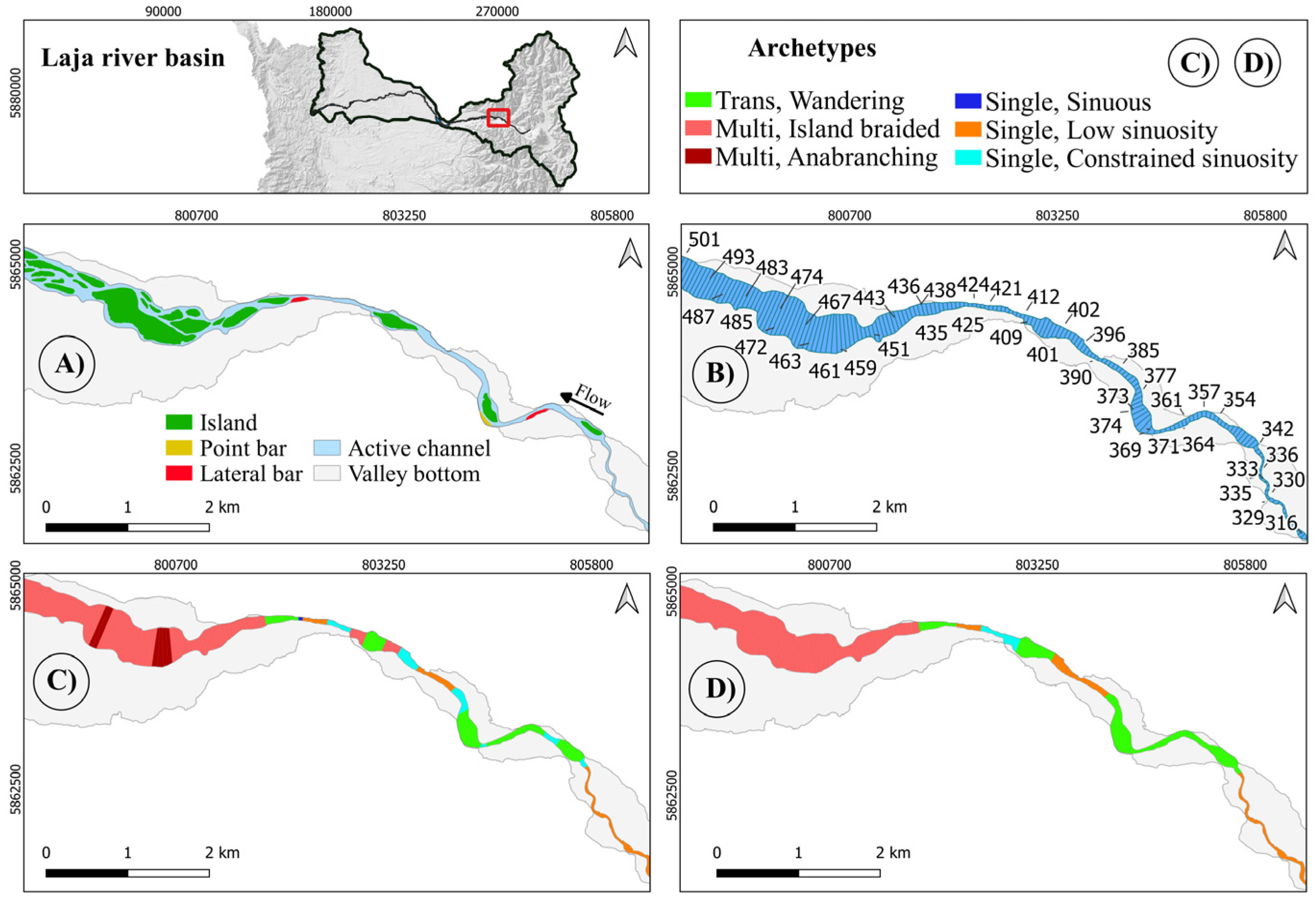
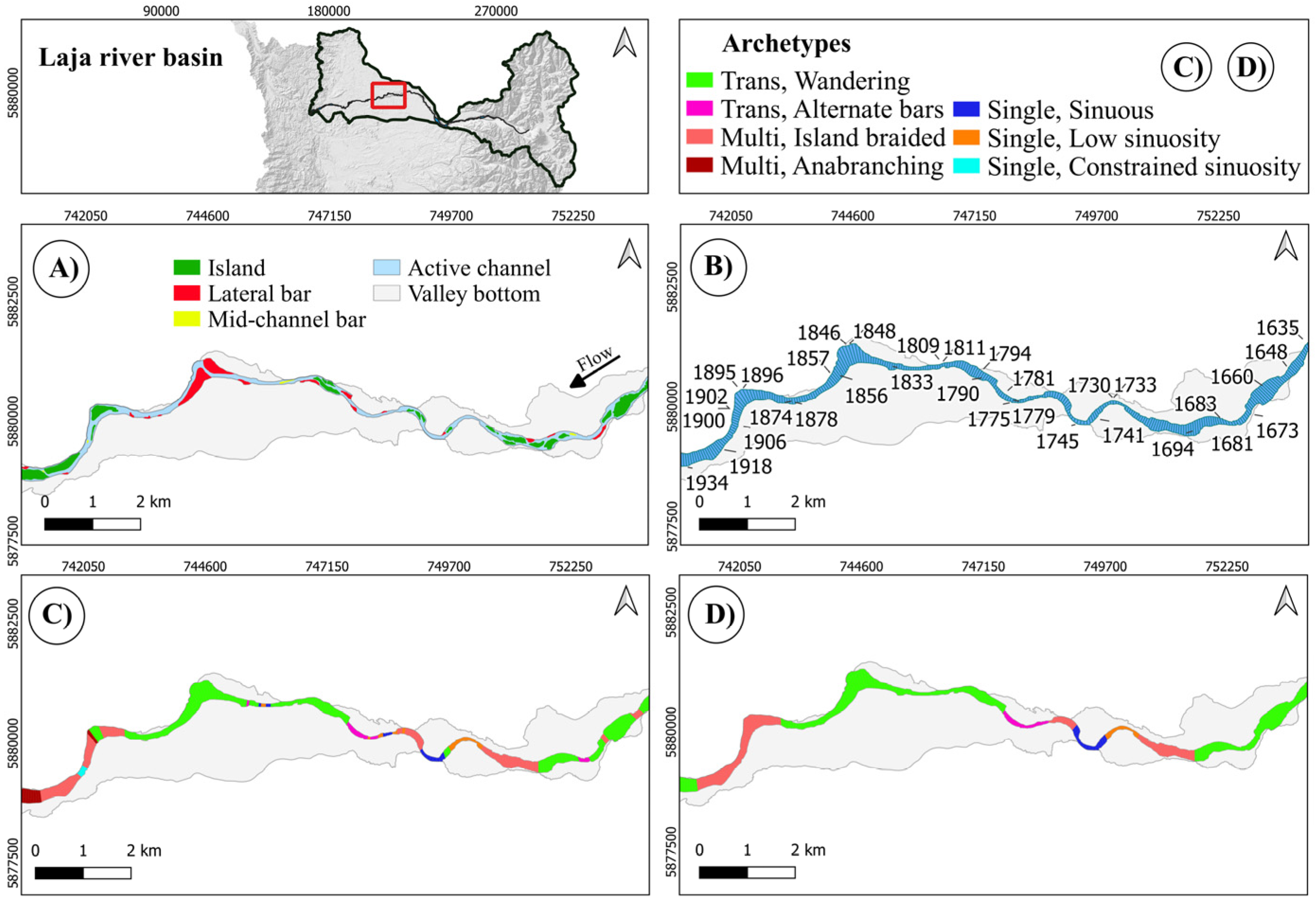
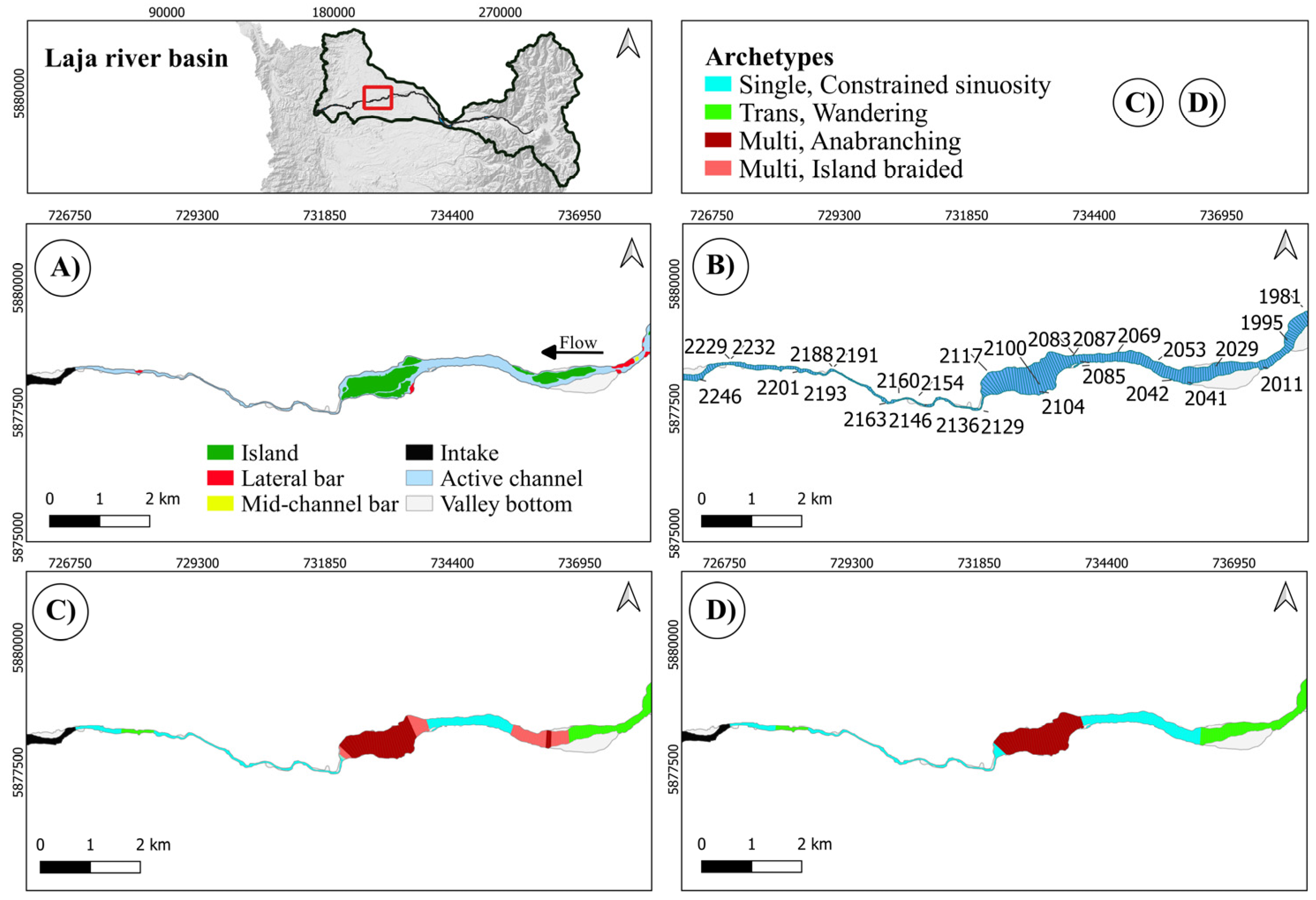
4.2. Laja River
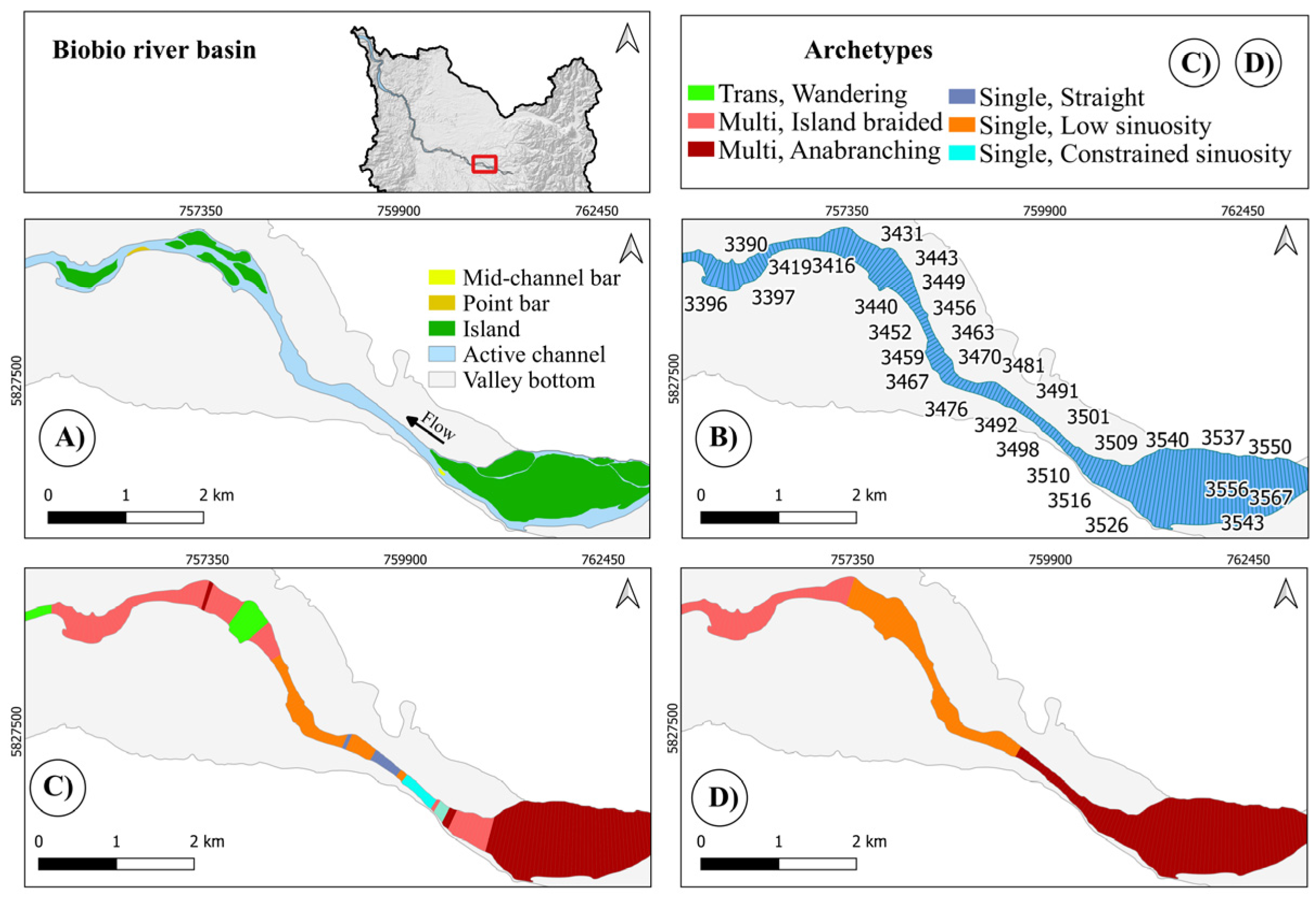
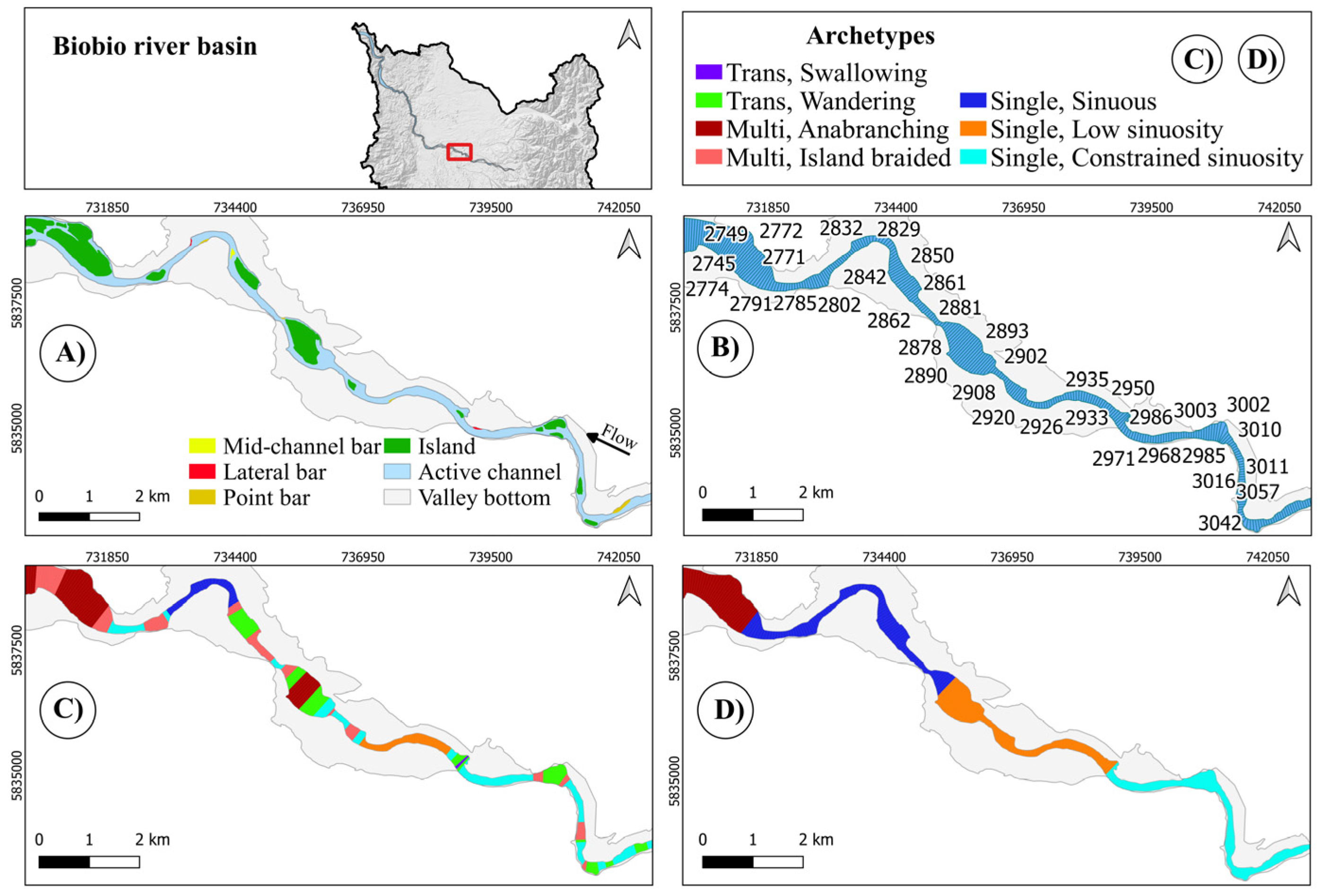
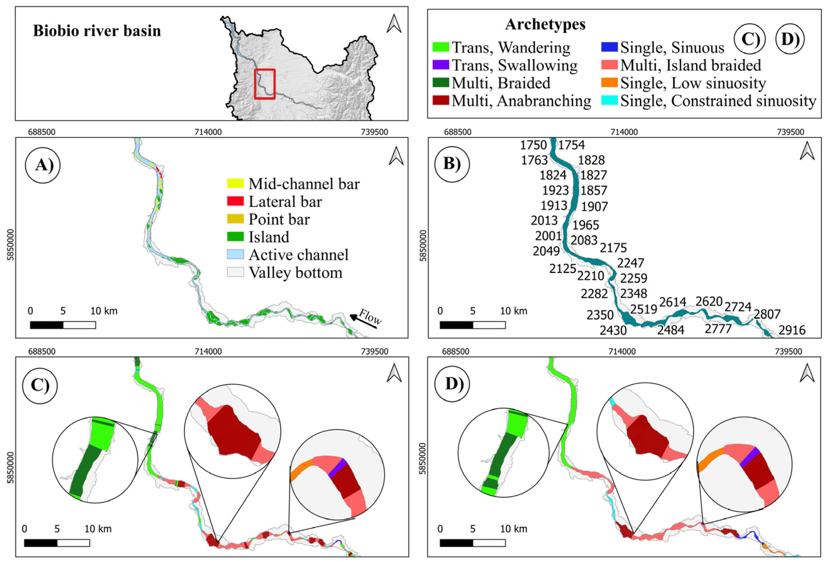
4.3. Biobío River
4.4. General Considerations
5. Conclusions
- -
- The ability to characterize large river networks;
- -
- The possibility of carrying out a regular, systematic monitoring of a river network to detect possible typological changes as clear indicators of (natural or anthropogenic) alterations that have occurred.
Author Contributions
Funding
Data Availability Statement
Acknowledgments
Conflicts of Interest
References
- Kondolf, G.M.; Piégay, H.; Schmitt, L.; Montgomery, D.R. Geomorphic classification of rivers and streams. In Tools in Fluvial Geomorphology; Wiley: Hoboken, NJ, USA, 2016; pp. 133–158. [Google Scholar] [CrossRef]
- Buffington, J.; Montgomery, D. Geomorphic classification of rivers. In Treatise on Geomorphology; Shroder, J., Wohl, E., Eds.; Elsevier: San Diego, CA, USA, 2013; Volume 9, pp. 730–767. [Google Scholar]
- Fryirs, K.; Brierley, G. Practical Applications of River Styles Framework as a Tool for Catchment-Wide River Management: A Case Study from Bega Catchment New South Wales; MacQuirie University: Auckland, New Zealand, 2005. [Google Scholar]
- Nardini, A.; Yépez, S.; Mazzorana, B.; Ulloa, H.; Bejarano, M.D.; Laraque, A. A systematic, automated approach for river segmentation tested on the Magdalena River (Colombia) and the Baker River (Chile). Water 2020, 12, 2827. [Google Scholar] [CrossRef]
- Parker, C.; Clifford, N.J.; Thorne, C.R. Automatic delineation of functional river reach boundaries for river research and applications. River Res. Appl. 2012, 28, 1708–1725. [Google Scholar] [CrossRef] [Green Version]
- Piégay, H.; Arnaud, F.; Belletti, B.; Bertrand, M.; Bizzi, S.; Carbonneau, P.; Dufour, S.; Liébault, F.; Ruiz-Villanueva, V.; Slater, L. Remotely sensed rivers in the Anthropocene: State of the art and prospects. Earth Surf. Process. Landf. 2020, 45, 157–188. [Google Scholar] [CrossRef]
- Dallaire, O.C.; Ouellet Dallaire, B.; Lehner, R.; Sayre, M. Thieme A multidisciplinary framework to derive global river reach classifications at high spatial resolution. Environ. Res. Lett. 2018, 14, 024003. [Google Scholar] [CrossRef]
- Demarchi, L.; Bizzi, S.; Piégay, H. Hierarchical object-based mapping of riverscape units and in-stream mesohabitats using LiDAR and VHR imagery. Remote Sens. 2016, 8, 97. [Google Scholar] [CrossRef] [Green Version]
- Bernard, T.G.; Davy, P.; Lague, D. Hydro-geomorphic metrics for high resolution fluvial landscape analysis. J. Geophys. Res. Earth Surf. 2022, 127, e2021JF006535. [Google Scholar] [CrossRef]
- Jézéquel, C.; Oberdorff, T.; Tedesco, P.A.; Schmitt, L. Geomorphological diversity of rivers in the Amazon Basin. Geomorphology 2022, 400, 108078. [Google Scholar] [CrossRef]
- Nardini, A.; Brierley, G. Automatic River Planform identification by a logical-heuristic algorithm. Geomorphology 2021, 375, 107558. [Google Scholar] [CrossRef]
- Frasson, R.P.d.M.; Pavelsky, T.M.; Fonstad, M.A.; Durand, M.T.; Allen, G.H.; Schumann, G.; Lion, C.; Beighley, R.E.; Yang, X. Global relationships between river width, slope, catchment area, meander wavelength, sinuosity, and discharge. Geophys. Res. Lett. 2019, 46, 3252–3262. [Google Scholar] [CrossRef] [Green Version]
- Beechie, T.; Imaki, H. Predicting natural channel patterns based on landscape and geomorphic controls in the Columbia River basin, USA. Water Resour. Res. 2014, 50, 39–57. [Google Scholar] [CrossRef]
- Beechie, T.J.; Liermann, M.; Pollock, M.M.; Baker, S.; Davies, J. Channel pattern and river-floodplain dynamics in forested mountain river systems. Geomorphology 2006, 78, 124–141. [Google Scholar] [CrossRef]
- Rabanaque, M.P.; Martínez-Fernández, V.; Calle, M.; Benito, G. Basin-wide hydromorphological analysis of ephemeral streams using machine learning algorithms. Earth Surf. Process. Landf. 2022, 47, 328–344. [Google Scholar] [CrossRef]
- Bertrand, M.; Piégay, H.; Pont, D.; Liébault, F.; Sauquet, E. Sensitivity analysis of environmental changes associated with riverscape evolutions following sediment reintroduction: Geomatic approach on the Drôme River network, France. Int. J. River Basin Manag. 2013, 11, 19–32. [Google Scholar] [CrossRef]
- Guillon, H.; Byrne, C.F.; Lane, B.A.; Sandoval Solis, S.; Pasternack, G.B. Machine learning predicts reach-scale channel types from coarse-scale geospatial data in a large river basin. Water Resour. Res. 2020, 56, e2019WR026691. [Google Scholar] [CrossRef]
- Horacio, J.; Ollero, A.; Pérez-Alberti, A. Geomorphic classification of rivers: A new methodology applied in an Atlantic Region (Galicia, NW Iberian Peninsula). Environ. Earth Sci. 2017, 76, 746. [Google Scholar] [CrossRef]
- Bizzi, S.; Lerner, D.N. Characterizing physical habitats in rivers using map-derived drivers of fluvial geomorphic processes. Geomorphology 2012, 169, 64–73. [Google Scholar] [CrossRef]
- Donadio, C.; Brescia, M.; Riccardo, A.; Angora, G.; Veneri, M.D.; Riccio, G. A novel approach to the classification of terrestrial drainage networks based on deep learning and preliminary results on solar system bodies. Sci. Rep. 2021, 11, 5875. [Google Scholar] [CrossRef]
- Alber, A.; Piégay, H. Spatial disaggregation and aggregation procedures for characterizing fluvial features at the network-scale: Application to the Rhône basin (France). Geomorphology 2011, 125, 343–360. [Google Scholar] [CrossRef]
- Nardini, A.; Yépez, S.; Bejarano, M.D. A Computer Aided Approach for River Styles—Inspired Characterization of Large Basins: A Structured Procedure and Support Tools. Geosciences 2020, 10, 231. [Google Scholar] [CrossRef]
- Hubert, P. The segmentation procedure as a tool for discrete modeling of hydrometeorological regimes. Stoch. Environ. Res. Risk Assess. 2000, 14, 297–304. [Google Scholar] [CrossRef]
- Brierley, G.; Fryirs, K. Geomorphology and River Management: Applications of the River Styles Framework; Blackwell Publishing: Malden, MA, USA, 2005. [Google Scholar] [CrossRef]
- Caamaño, D. Caracterización de cambios morfológicos en la parte media del río Biobío. Master’s Thesis, Universidad Católica de la Santísima Concepción, Concepción, Chile, 2019. [Google Scholar]
- Niemeyer, H. Hoyas hidrográficas de Chile: 8a. Región del Bío-Bío, 9a. Región de la Araucanía, 10a. Región de Los Lagos. 1980. Available online: https://bibliotecadigital.ciren.cl/handle/20.500.13082/2348 (accessed on 1 February 2023).
- Mardones, M.; Vargas, J. Efectos hidrológicos de los usos eléctrico y agrícola en la cuenca del río Laja (Chile centro-sur). Rev. Geogr. Norte Gd. 2005, 33, 89–102. [Google Scholar]
- Yépez, S.; Salas, F.; Nardini, A.; Valenzuela, N.; Osores, V.; Vargas, J.; Rodriguez, R.; Piégay, H. Semi-automated morphological characterization using South Rivers Toolbox. Proc. IAHS 2023, 100, 1–8. [Google Scholar]
- McFeeters, S.K. The use of the Normalized Difference Water Index (NDWI) in the delineation of open water features. Int. J. Remote Sens. 1996, 17, 1425–1432. [Google Scholar] [CrossRef]
- Gilbert, J.T.; Macfarlane, W.W.; Wheaton, J.M. The Valley Bottom Extraction Tool (V-BET): A GIS tool for delineating valley bottoms across entire drainage networks. Comput. Geosci. 2016, 97, 1–14. [Google Scholar] [CrossRef]
- Kleinhans, M.G.; van den Berg, J.H. River channel and bar patterns explained and predicted by an empirical and a physics-based method. Earth Surf. Process. Landf. 2011, 36, 721–738. [Google Scholar] [CrossRef]
- Ashworth, P.J.; Lewin, J. How do big rivers come to be different? Earth-Sci. Rev. 2012, 114, 84–107. [Google Scholar] [CrossRef]


| N | River | Year | L (km) | wmax (m) | wmin (m) | A. Basin (km2) | Qav (m3/s) | N. Macrosegments |
|---|---|---|---|---|---|---|---|---|
| 1 | Duqueco | 2009 | 102 | 634 | 11 | 1551 | 55 | 4 |
| 2 | Laja | 2019 | 140 | 44 | 5 | 4667 | 151 | 5 |
| 3 | Biobío | 2020 | 198 (*) | 2649 | 15 | 24,273 | 984 | 5 |
Disclaimer/Publisher’s Note: The statements, opinions and data contained in all publications are solely those of the individual author(s) and contributor(s) and not of MDPI and/or the editor(s). MDPI and/or the editor(s) disclaim responsibility for any injury to people or property resulting from any ideas, methods, instructions or products referred to in the content. |
© 2023 by the authors. Licensee MDPI, Basel, Switzerland. This article is an open access article distributed under the terms and conditions of the Creative Commons Attribution (CC BY) license (https://creativecommons.org/licenses/by/4.0/).
Share and Cite
Nardini, A.G.C.; Salas, F.; Carrasco, Z.; Valenzuela, N.; Rojas, R.; Vargas-Baecheler, J.; Yépez, S. Automatic River Planform Recognition Tested on Chilean Rivers. Water 2023, 15, 2539. https://doi.org/10.3390/w15142539
Nardini AGC, Salas F, Carrasco Z, Valenzuela N, Rojas R, Vargas-Baecheler J, Yépez S. Automatic River Planform Recognition Tested on Chilean Rivers. Water. 2023; 15(14):2539. https://doi.org/10.3390/w15142539
Chicago/Turabian StyleNardini, Andrea Gianni Cristoforo, Francisca Salas, Zoila Carrasco, Noelia Valenzuela, Renzo Rojas, José Vargas-Baecheler, and Santiago Yépez. 2023. "Automatic River Planform Recognition Tested on Chilean Rivers" Water 15, no. 14: 2539. https://doi.org/10.3390/w15142539