Article

Incorporating Wetland Delineation and Impacts in Watershed-Scale Hydrologic Modeling

1
Department of Civil, Construction and Environmental Engineering (Dept. 2470), North Dakota State University, P.O. Box 6050, Fargo, ND 58108-6050, USA
2
Wet Ecosystem Research Group, Department of Biological Sciences (Dept. 2715), North Dakota State University, P.O. Box 6050, Fargo, ND 58108-6050, USA
3
Department of Agricultural and Biosystems Engineering (Dept. 7620), North Dakota State University, P.O. Box 6050, Fargo, ND 58108-6050, USA
*
Author to whom correspondence should be addressed.
Water 2023, 15(14), 2518; https://doi.org/10.3390/w15142518
Submission received: 12 June 2023 / Revised: 26 June 2023 / Accepted: 6 July 2023 / Published: 9 July 2023
(This article belongs to the Special Issue Wetland Processes, Monitoring and Modeling for Design and Management)

Abstract

:
In semi-distributed hydrologic models, it is difficult to account for the impacts of wetlands on hydrologic processes, as they are based on lumped, subbasin-scale wetland concepts. It is a challenge to incorporate the influences of individual small wetlands into watershed-scale models by using lumped parameterization. The objective of this study was to improve watershed-scale hydrologic modeling by taking into account real wetland features during the wetland parameterization. To achieve this objective, a joint modeling framework was proposed to couple a surface delineation algorithm with a semi-distributed hydrologic model and then applied to the Upper Turtle River watershed in North Dakota, USA. The delineation algorithm identified the topographic properties of wetlands, which were further utilized for wetland parameterization. A nonlinear area–storage relationship was determined and used in the estimation of the wetland-related parameters. The results demonstrated that the new joint modeling approach effectively avoided misestimating the wetland-related parameters by accounting for real topographic characteristics (e.g., storage, ponding area, and contributing area) of identified wetlands and their influences, and provided improved modeling of the hydrologic processes in such a wetland-dominated watershed.

1. Introduction

Wetlands play a significant role in watershed hydrologic processes, and watershed hydrologic models are useful tools to assess their impacts [1,2,3]. Wetlands can alter watershed water balance by affecting surface runoff generation and other hydrologic processes [4,5,6,7,8,9,10,11]. The effects of wetlands vary because of the diversity of wetland topographic features [4,5,7,10]. For instance, using a semi-distributed hydrologic model, Evenson et al. [6] found that compared with smaller wetlands, larger wetlands acted as hydrologic “gatekeepers” that prevented surface runoff from reaching streams. Martinez-Martinez et al. [10] revealed that the areas of wetland had significant impacts on streamflow, while the depths of wetland did not. Golden et al. [7] found that wetlands farther away from a stream had greater capacity for increasing streamflow than those closer, due to the sequencing of watershed hydrologic connectivity in their study area. Blanchette et al. [4] found that contributing area was important for a wetland to provide hydrologic services, especially for mitigating extreme stream flows. Thus, the variability in the size, spatial distribution, and contributing area of wetlands makes their hydrologic functions and influences more complicated.
Watershed hydrologic modeling facilitates the assessment of the impacts of wetlands and their losses or restorations [6,9,10,12]. Evenson et al. [6] conducted hydrologic modeling for different wetland scenarios, showing a consistent potential of increased downstream flooding from wetland losses. Lee et al. [9] found that wetland losses reduced the baseflow contribution and increased the inter-monthly variability of downstream flow, especially during extreme flow conditions. Martinez-Martinez et al. [10] showed that wetland restorations had a negligible impact on the long-term average daily peak flow, but only had slight impacts on the reduction in average annual maximum peak flow. Wetlands have been widely acknowledged as providing critical ecosystem services to humans, yet they have also been destroyed and altered by human activities at very high rates around the world [13]. In recent decades, the restoration and creation of wetlands have become important means to mitigate some of that damage [14]. It is therefore of great importance that the impacts on watershed hydrologic processes of changes in wetland sizes and distributions can be accurately assessed and predicted, not only because of loss of wetlands but also due to addition of newly constructed wetlands.
Watershed hydrologic models have been used to assess the impacts of wetland losses and restorations (e.g., [4,15,16,17,18,19,20,21,22,23]). Among the existing hydrologic models, the Soil and Water Assessment Tool (SWAT) with a built-in wetland module has been widely employed and/or modified for wetland-based hydrologic modeling [2,5,6,9,10,24,25,26,27,28,29]. The wetland module incorporated in SWAT depicts wetland hydrologic processes at a subbasin level using a lumped concept. To perform wetland routing, several wetland-related parameters are required to calculate the inflow, outflow, and seepage of the lumped wetland. However, the oversimplified, subbasin-scale wetland with the lumped parameters hinders the application of SWAT, especially in complex wetland systems such as the Prairie Pothole Region (PPR) [30]. It is particularly difficult to assess the impacts of wetlands on hydrologic processes using SWAT without accurate estimation of the wetland-related parameters. Liu et al. [31] found that the lack of accurate hydraulic conductivity of the wetland bottom resulted in overestimation of percolation.
Various approaches have been used to estimate wetland parameters in SWAT, including the fraction of the subbasin area draining into the lumped wetlands (Fr), four shape parameters of the lumped wetlands (i.e., maximum surface area (SAmx), maximum storage volume (Vmx), normal surface area (SAnor), and normal storage volume (Vnor)), and the effective saturated hydraulic conductivity of the lumped wetland bottoms (Kwet) [1,2,3,10,11,27,29,32]. Due to the lack of real data, many studies simply utilized some assumed values. For example, an assumed wetland depth is used to determine the wetland volume parameters [2,3]. Similarly, the hydraulic conductivity of the wetland bottom is frequently assumed as zero [1,2]. Alternatively, the wetland parameters are estimated based on the limited data from field survey or surface delineation tools. Wang et al. [29] estimated the soil saturated hydraulic conductivity of the entire watershed from a field survey and set it as the hydraulic conductivity of the wetland bottom. To some extent, these methods made certain improvements to wetland modeling by incorporating the actual wetland topographic features. However, to the best of our knowledge, few studies have accounted for the dissimilar properties of real wetlands in the estimation of Vnor and SAnor. Instead, Vnor was assumed as constant proportions of Vmx and SAnor was assumed as constant proportions of SAmx across different subbasins [1,2,3,11,29,32]. Thus, there is room for improvement to apply such methods to wetland-dominated watersheds.
The current work was part of a collaborative study that addressed the overall question of how much wetland is needed within a watershed to significantly reduce sediment and pollutant loads downstream. To answer this question, the first step was to improve existing hydrologic models regarding hydrologic functioning of wetlands. Therefore, the objective of this study was to improve the hydrologic modeling in a wetland-dominated watershed by taking into account real wetland features through wetland parameterization. To achieve this objective, a joint modeling framework was proposed to couple the Hydrologic Units Delineation for Depressions and Channels (HUD-DC) [33] with SWAT. HUD-DC was used to identify wetlands and their spatial distributions, maximum ponding areas, maximum storage, and contributing areas, while SWAT was utilized for watershed hydrologic modeling. A new procedure was proposed for wetland parameterization by coupling HUD-DC and SWAT. Here, the joint modeling approach was applied to the wetland-dominated Upper Turtle River (UTR) watershed in North Dakota, USA.

2. Materials and Methods

2.1. Overall Modeling Framework

To enhance the wetland module in SWAT, a joint modeling framework, which coupled HUD-DC with SWAT, was proposed (Figure 1). In this framework, the wetland parameters in SWAT were estimated based on the topographic features of the wetlands identified by HUD-DC. A three-step modeling procedure was performed: (1) surface delineation, (2) wetland parameterization, and (3) SWAT modeling (Figure 1). In step 1, watershed delineation was performed using ArcSWAT [34] and wetland delineation was performed using HUD-DC. The subbasin features were obtained based on the fully filled digital elevation model (DEM) during the watershed delineation, while the wetland topographic properties of each subbasin were extracted from the fully filled DEM, the original DEM [35], and the National Wetland Inventory data [36] during wetland delineation. In step 2, wetland parameterization was performed by coupling HUD-DC and SWAT. In step 3, SWAT modeling enhanced by the results from step 2 was performed. As detailed in the following subsection, this new procedure of wetland parameterization takes full advantage of the combination of the delineation results from both ArcSWAT and HUD-DC and the soil properties from the SWAT database, which ensures that the parameters used for the routing of the wetlands reflect their actual conditions.

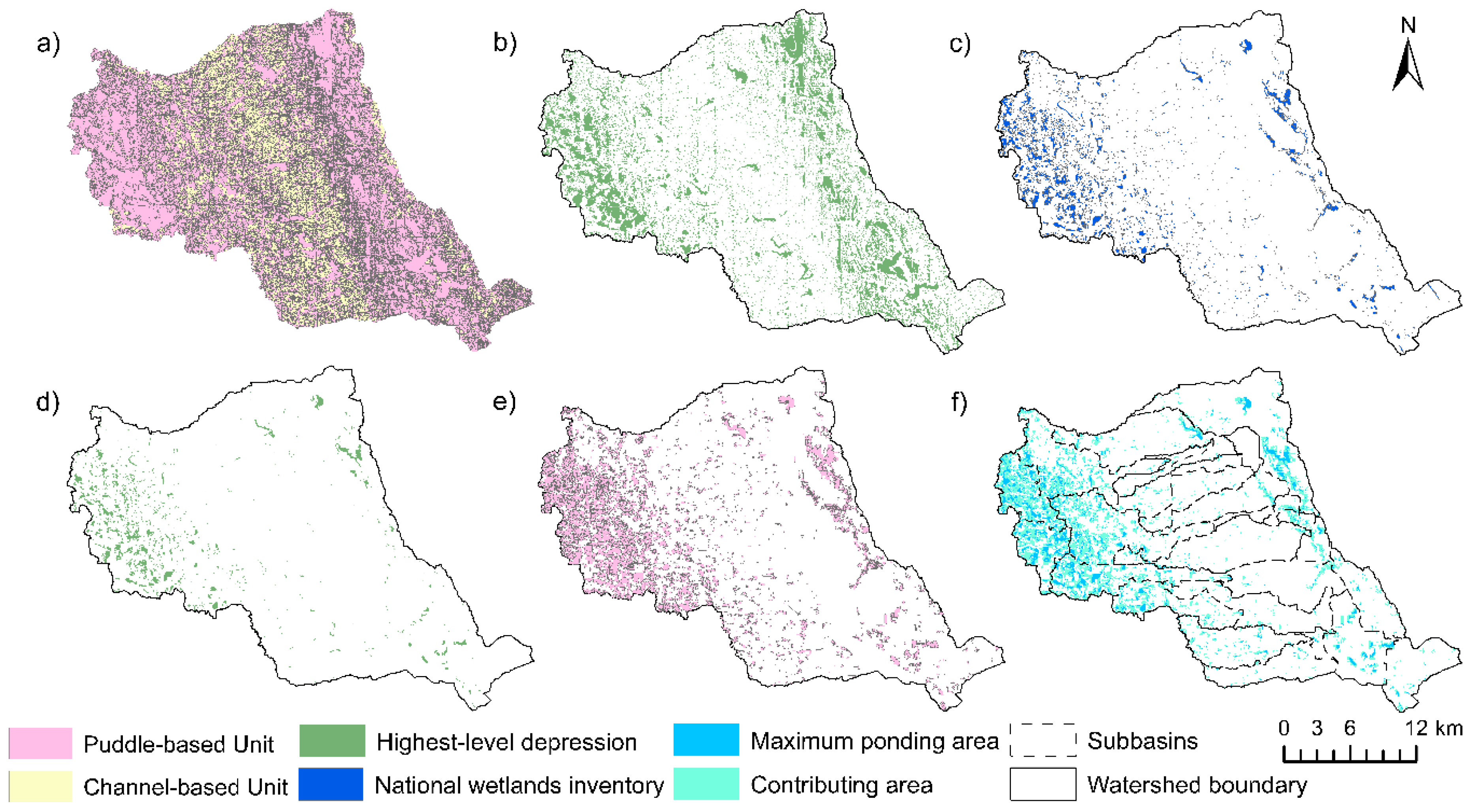
2.2. HUD-DC Wetland Delineation

HUD-DC [33] is an ArcGIS-based tool developed mainly for topographic delineation with a focus on identifying surface depressions and channels. The algorithm of HUD-DC was primarily based on the depression-oriented delineation methods [37,38,39]. The related delineation approaches and algorithms have been widely tested over a decade in a series of depression-oriented hydrologic modeling studies (e.g., [33,37,38,39,40,41,42,43]). Based on both the original DEM and the fully filled DEM, HUD-DC identifies depressions, channels, and their contributing areas as two types of hydrologic units (i.e., puddle-based units and channel-based units), as well as the connectivity between the hydrologic units. HUD-DC implements the depression identification module and the channel and unit identification module successively. The depression identification module consists of four major steps: (1) identifying the filled cells, (2) searching for potential depressions, (3) removing the fault depression cells, and (4) determining the final depressions. The filled cells are identified based on the elevation difference between the original DEM and the fully filled DEM. Then, the adjacent filled cells are assigned mutual IDs based on the elevation of the filled DEM, where the cells with a mutual ID are considered a potential depression. For each potential depression, the cells without hydrologic connectivity with other cells are removed. Finally, each modified potential depression is identified as the final depression and its threshold(s) are also identified. Note that since the focus on the surface delineation is at the watershed scale, only the highest-level depressions are identified, which may contain various lower-level depressions that potentially merge during rainfall/snowmelt events. In the channel and unit identification module, channels, puddle-based units, channel-based units, and the connectivity between the hydrologic units are identified. The channels and their ending points are determined based on the fully filled DEM. The “Watershed” function in ArcGIS is employed to delineate the puddle-based units based on the depression thresholds and the channel-based units based on the channel ending points. Finally, the IDs of the depressions and channels are assigned to their associated hydrologic units. In this study, HUD-DC was utilized to delineate the topographic features of wetlands, including their spatial distributions, maximum ponding areas, maximum storage, and contributing areas.

2.3. Introduction to SWAT Modeling

SWAT is a semi-distributed, physically based hydrologic model where a watershed is generally divided into a number of subbasins [44], each of which is further divided into many hydrologic response units (HRUs). The impoundment water routing is not considered in SWAT because the watershed delineation is based on the fully filled DEM. Instead, SWAT allows off-channel impoundment water routing at the subbasin level based on a lumped pond/wetland concept. Thereafter, channel routing is performed throughout the drainage network. In the wetland module of SWAT, the aggregate of surface runoff and lateral flow is divided into two components, which are determined by a fraction parameter of the lumped wetland. The first component is summed to the subbasin outlet directly, while the second one is routed through the lumped wetland before it is divided into two parts. The first part is added to the subbasin outlet as the wetland outflow, which is determined by using four shape parameters of the lumped wetland. The second part is added to groundwater as wetland seepage, which is determined by the effective saturated hydraulic conductivity of the lumped wetland bottom.
In the wetland module, four shape parameters are used to determine the area–storage relationship of the lumped wetland. The outflow and the storage volume of the lumped wetland of a subbasin at any daily time step are given by [28,44]:
V o u t j , k = 0                                                                                     i f                                     V j , k < V n o r j V j , k V n o r j 10                                                       i f       V n o r j V j , k V m x j V j , k V m x j                                               i f                                       V j , k > V m x j                                
in which
V j , k = V j , k 1 + ( F r j × A s u b j S A j , k ) × q s u b j , k + R j , k × S A j , k 0.6 × E T o j , k × S A j , k K w e t j × S A j , k × T
  V j , k + 1 = V j , k V o u t j , k
where V o u t j , k is the outflow volume of the lumped wetland of subbasin j at time step k [L3], V j , k is the volume of the water stored in the lumped wetland of subbasin j at time step k [L3], V n o r j is the normal storage of the lumped wetland of subbasin j [L3], V m x j is the maximum storage of the lumped wetland of subbasin j [L3], V j , k 1 is the volume of the water stored in the lumped wetland of subbasin j at time step k-1 [L3], F r j is the fraction of the subbasin area draining into the lumped wetland of subbasin j, A s u b j is the area of subbasin j [L2], S A j , k is the ponding area of the lumped wetland of subbasin j at time step k, which is determined by the area–storage relationship [L2], q s u b j , k is the surface runoff and lateral flow in subbasin j at time step k [L], R j , k is the precipitation of subbasin j at time step k [L], E T o j , k is the potential evapotranspiration from subbasin j at time step k [L], K w e t j is the effective saturated hydraulic conductivity of the lumped wetland bottom of subbasin j [L/T], T is the time step length [T], and V j , k + 1 is the volume of the water stored in the lumped wetland of subbasin j at time step k+1 [L3].

2.4. Wetland Parameterization

The wetland parameters in SWAT were estimated by coupling HUD-DC and SWAT. The distribution and areas of subbasins from the watershed delineation in ArcSWAT and the soil properties from the SWAT database were required. Based on the subbasin distribution, the ID, spatial distribution, maximum ponding area, maximum storage, and contributing area of each individual wetland in a subbasin were derived from the HUD-DC wetland delineation results. Since the wetland routing in SWAT modeling was at the subbasin level, the wetland parameterization was also performed for each subbasin.
As Fr determines how much surface runoff and lateral flow from a subbasin will flow into its lumped wetland [28], it can be defined as the ratio of the ponding and contributing area of all wetlands in a subbasin to the corresponding subbasin area with an assumption of a spatially even generation of surface runoff and lateral flow among different HRUs within the subbasin. Thus, the Fr of a subbasin can be estimated by:
F r j = i = 1 n ( A m p a i , j + A c a i , j ) / A s u b j
where n is the total number of real wetlands in subbasin j, A m p a i , j is the maximum ponding area of the real wetland i in subbasin j [L2], and A c a i , j is the contributing area of the real wetland i corresponding to its maximum ponding area in subbasin j [L2]. The shape parameters of the lumped wetland SAmx and Vmx for a subbasin can be expressed as:
S A m x j = i = 1 n A m p a i , j
V m x j = i = 1 n V m s i , j  
where V m s i , j is the maximum storage of the real wetland i in subbasin j [L3].
According to Equation (1), the lumped wetland will not release outflow until the stored water volume reaches its Vnor. In this study, when any real wetland begins to release its outflow, the stored water volume of all real wetlands in a subbasin was considered as the Vnor of the corresponding lumped wetland. To identify the timing of water release for real wetlands, their maximum ponding areas, maximum storage, and contributing areas were utilized. For a real individual wetland, the time when its maximum storage was fully filled by the surface runoff and lateral flow from its contributing area and the rainfall on its maximum ponding area was assumed as the time when it began to release outflow. The smaller the storage and the larger the maximum ponding and contributing area, the shorter the time required for the filling process. To identify the real wetland with the shortest time, a ratio of the maximum storage to the maximum ponding and contributing area (i.e., storage-area ratio) of each wetland was calculated. The individual wetland with the minimum storage-area ratio was considered as the wetland with the shortest filling time and the earliest outflow release. When it begins to release its outflow, the storage of all wetlands in subbasin j (Vnor j) can be estimated as the product of their maximum ponding and contributing areas and the minimum storage-area ratio, as described in Equation (7):
V n o r j = r S A m i n j × i = 1 n ( A m p a i , j + A c a i , j )
in which
r S A m i n j = m i n r S A 1 , j , r S A 2 , j ,   , r S A i , j ,     r S A i + 1 , j ,   ,   r S A n , j  
r S A i , j = V m s i , j / ( A m p a i , j + A c a i , j )  
where r S A m i n j is the minimum storage-area ratio in subbasin j [L], and r S A i , j is the storage-area ratio of the real wetland i in subbasin j [L]. SAnor is the ponding area of the lumped wetland when the water storage reaches its Vnor. To estimate SAnor for a subbasin, the quantitative correlation between the accumulative maximum storage and the accumulative maximum ponding area of all individual wetlands in the subbasin was determined based on the wetland delineation results from HUD-DC. Thus, SAnor for a subbasin was estimated by the quantitative correlation and Vnor.
Kwet was estimated as the weighted average of the hydraulic conductivity values of the soils under the real wetlands, which were gained from the SWAT database. Thus, Kwet of a subbasin is given by:
K w e t j = i = 1 n l = 1 m K s o l l , i , j × A s o l l , i , j i = 1 n A m p a i , j  
where m is the total number of soil types of the top soil layer under the real wetland i in subbasin j, K s o l l , i , j is the hydraulic conductivity of soil type l under real wetland i in subbasin j [L/T], and A s o l l , i , j is the area of soil type l under real wetland i in subbasin j [L2].

2.5. Study Area and Model Setup

In this study, the UTR watershed in North Dakota, USA (Figure 2) was selected to test the performance of the joint modeling framework. The UTR watershed covers an area of 664.24 km2, including parts of Grand Forks and Nelson counties in North Dakota, and drains to the outlet located at the USGS gaging station 05082625 Turtle River at Turtle River State Park near Arvilla, ND (47°55′55″ N, 97°30′51″ W). The surface elevation varies from 293 to 481 m across the watershed. Based on the 2019 NLCD (National Land Cover Database), the UTR watershed is mainly covered by agricultural land (67.03%) and wetland (8.92%).
A 10 m DEM and the reservoir distribution data (Figure 2) were used for watershed delineation. The DEM was obtained from the USGS 3D Elevation Program and the reservoir data were obtained from the ND Department of Water Resources (Table 1). A two-step delineation procedure was performed by using the “Watershed Delineator” in ArcSWAT. In the first step, the DEM-based method was selected for stream definition and 23 subbasins were identified. Then, the distributions of the identified subbasins were compared with the distribution of reservoirs. Note that a “reservoir” in SWAT model is only allowed to be located at the stream network node (i.e., subbasin outlet). Based on the distribution of reservoirs, four more subbasin outlets were added manually during the second-step delineation, which resulted in 27 subbasins.
During HRU analysis, the LULC data from the National Land Cover Database, soil types from the Soil Survey Geographic (SSURGO) Database, and the slopes generated from the DEM were utilized. The selected thresholds were 5% for LULC, 10% for soil, and 0% for slope [49]. Eventually, 631 HRUs were defined based on the reclassified 15 LULC types, 182 soil types, and 3 slopes. Meanwhile, the curve numbers for all HRUs were determined for surface runoff simulation for each HRU, except for the HRUs defined by water LULC.
HUD-DC was used to gain wetland topographic properties based on the DEM and the National Wetlands Inventory (NWI) data. The DEM with a horizontal resolution of 10 m was selected for this watershed-scale modeling [30]. The NWI data were used for wetland delineation. To complete the wetland delineation for a subbasin, the original DEM was first clipped by the subbasin shapefile to obtain the clipped DEM within the subbasin. Secondly, the clipped DEM was clipped by the NWI to obtain the clipped DEM within the NWI, which was used to determine the ID, spatial distribution, maximum ponding area, and maximum storage of each wetland using the depression identification module in HUD-DC. Finally, using the channel and unit identification module in HUD-DC, the contributing area of each wetland was identified based on the results from the depression identification module and the clipped DEM within the subbasin. Following the methods for wetland parameterization, the wetland delineation results from HUD-DC and the soil profile in the SWAT database generated from the SSURGO database were utilized to estimate the wetland-related parameters for all subbasins.
The variable storage routing method in SWAT was selected for channel routing. Based on the reservoir information from NDDWR, the reservoir parameters in the SWAT model were estimated. The daily precipitation and maximum and minimum temperature data were downloaded from the Parameter-elevation Regressions on Independent Slopes Model (PRISM), and daily solar radiation, wind speed, and relative humidity data were downloaded from the Prediction Of Worldwide Energy Resources (POWER) Data Access Viewer.
Using the observed discharge data at the watershed outlet obtained from the USGS National Water Information System [50], the SWAT-CUP (Calibration Uncertainty Program) [51] was employed for calibration and validation of the joint model. Specifically, the SUFI-2 (Sequential Uncertainty Fitting, version 2) algorithm [52] was utilized for the calibration and uncertainty analysis. The entire modeling consisted of a 1-year period (2010) for warmup, a 3-year period (2011–2013) for calibration, and a 4-year period (2014–2017) for validation. Two statistical metrics were used to assess the model performance: (1) Nash–Sutcliffe efficiency (NSE) [53], which has been widely used to evaluate the performances of hydrologic models, and (2) percentage bias (PBIAS). The NSE and PBIAS, respectively, are given by:
N S E = 1 k = 1 p ( O k S k ) 2 k = 1 p ( O k O ¯ ) 2
P B I A S = k = 1 p ( O k S k ) × 100 k = 1 p ( O k )
where p is the total number of time steps, O k is the observed discharge at time step k [L3/T], S k is the simulated discharge at time step k [L3/T], and O ¯ is the mean observed discharge [L3/T].
To demonstrate the improved capabilities of the coupled HUD-DC and SWAT modeling system, two other SWAT models were also developed for the UTR watershed. In comparison model 1 (CM1), an original SWAT without the support of the delineation results from HUD-DC was developed. In CM1, the spatial distribution and areas of the wetlands were gained from the LULC data and utilized during the HRU analysis to reflect the impacts of wetlands as wetland HRUs, instead of simulating using the wetland module. Furthermore, to demonstrate the benefits of the proposed estimation methods for Vnor and SAnor, comparison model 2 (CM2) was also developed, in which the wetland-related parameters were estimated using the same method as the joint model, except that Vnor and SAnor were assumed to be the same as the corresponding Vmx and SAmx [29,32].

3. Results and Discussion

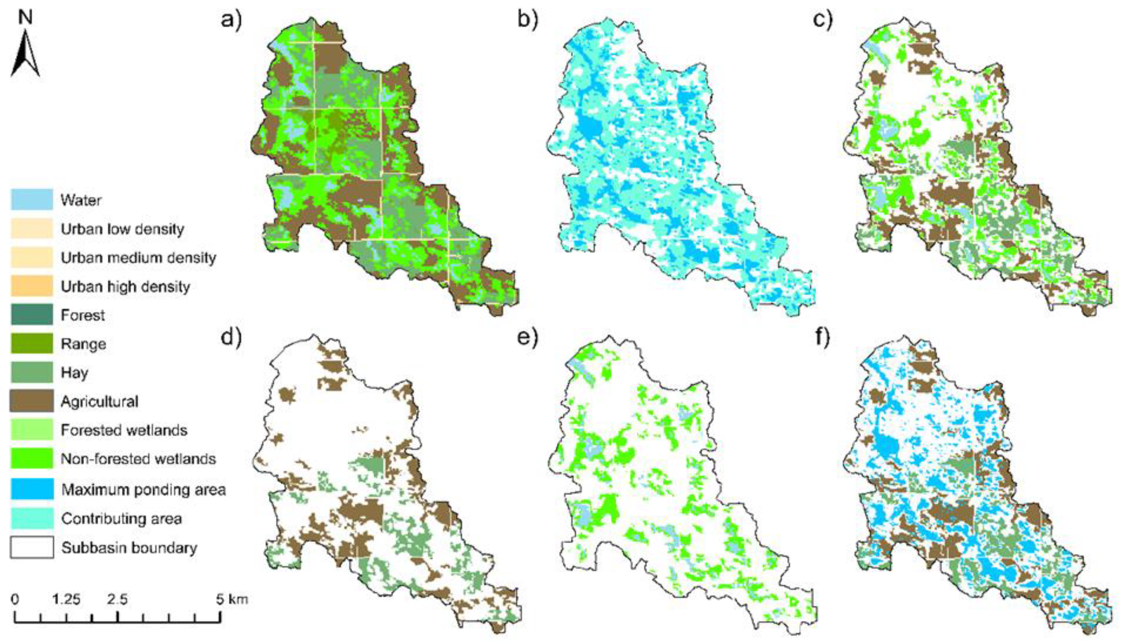
3.1. Delineation of Wetlands

Based on the delineation results from HUD-DC, puddle-based units (Figure 3a), channel-based units (Figure 3a), and highest-level depressions (Figure 3b) were identified. Based on the DEM clipped by the wetland polygon of the NWI (Figure 3c), the highest-level depressions within the NWI wetland area accounted for an area of 29.34 km2 (Figure 3d). Thus, the area of the corresponding puddle-based units was 118.63 km2 (Figure 3e). Finally, the maximum ponding areas and contributing areas of 5786 individual wetlands across 27 subbasins in the UTR watershed were determined (Figure 3f).
Table 2 lists the wetland topographic properties for all subbasins determined by HUD-DC. The number of wetlands and their maximum ponding areas, maximum storage, and contributing areas varied among the 27 subbasins. The total maximum ponding area accounted for 4.42% of the watershed area and the total contributing area of the wetlands accounted for 13.44% of the watershed area, indicating that the surface runoff generated from 17.86% of the watershed area flows into the wetlands. In subbasin 12, the proportion of the total maximum ponding and contributing area to the subbasin area was as high as 71.23%.

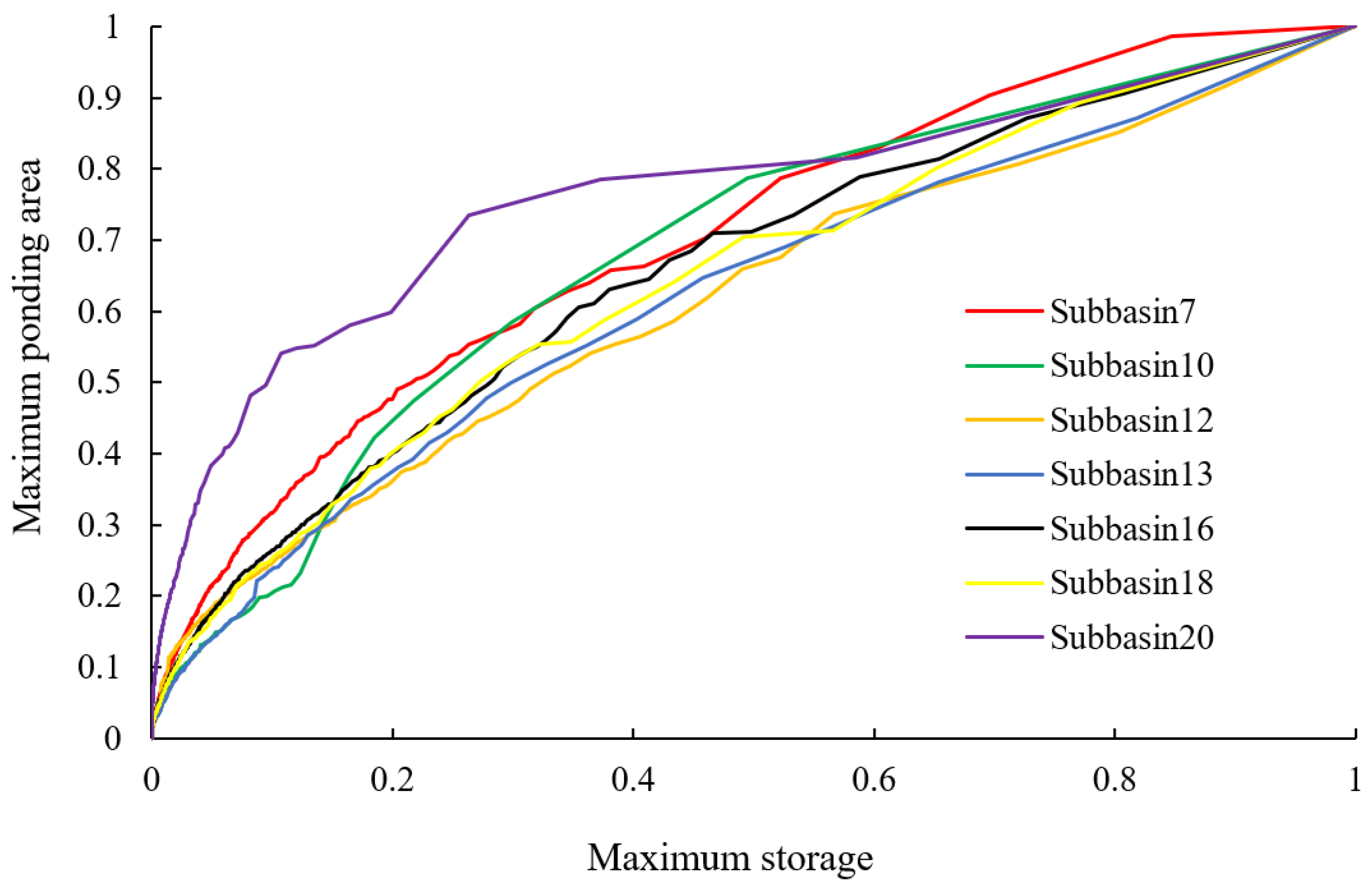
3.2. Wetland-Related Parameters

Based on the wetland topographic properties at the subbasin level (Table 2), the wetland-related parameters used in the SWAT model were estimated using the wetland parameterization method proposed in this study. The results are shown in Table 3. Since the proportions of total maximum ponding and contributing areas of the 27 subbasins ranged from 0.30% to 71.23%, the estimated values of Fr varied from 0.003 to 0.712. Estimated by their maximum ponding areas and the maximum storage of all wetlands (Table 2), Vmx ranged from 140 m3 to 5.48 × 10⁶ m3 and SAmx ranged from 0.1 ha to 477.4 ha for all subbasins (Table 3). Based on the maximum ponding area, maximum storage, and contributing areas of all individual wetlands in a subbasin, Vnor was calculated using Equations (7)–(9) for all subbasins, ranging from 1.3 m3 to 278.8 m3 (Table 3). In addition, the area–storage relationships of individual wetlands of all subbasins were derived from the maximum ponding areas and maximum storage of the wetlands (Figure 4) and utilized to estimate the corresponding SAnor, which ranged from 0.1 ha to 2.1 ha (Table 3).

3.3. Joint Model Performance for Wetland-Influenced Areas

A total of 17 parameters were selected for the calibration of the joint model since they had smaller p-values and, in particular, the simulated outlet discharge was found to be more sensitive to these 17 parameters. Table 4 lists the calibrated values or ranges of the 17 parameters.
Figure 5 shows the comparison of the hydrographs simulated by the joint model against the observed data. Its performance was evaluated by using two statistical metrics for both calibration and validation periods (Table 5). The NSE values are 0.82 for the calibration period and 0.61 for the validation period and the PBIAS values are 5.01% for the calibration period and 6.50% for the validation period, indicating that the model performance is “very good” in the calibration period and “satisfactory” in the validation period [54]. In the entire simulation period (2011–2017), the UTR watershed received an average annual precipitation of 582.7 mm, which generated 84.9 mm surface runoff. The average annual evapotranspiration, as the major loss term of the watershed, was 493.8 mm. In addition, 76.2 mm water flowed out of the watershed through its outlet. On average, surface runoff contributed 74% of the streamflow, while the remaining 26% of the streamflow came from baseflow. Figure 5 shows slight underestimations, especially for the early spring peaks induced by snowmelt in some years (e.g., 2013, 2014, and 2017), which can be attributed to the limited capability of SWAT in simulating complex hydrologic processes in cold regions. Similar issues were also observed by Tahmasebi Nasab et al. [55], Zeng et al. [30], and Shabani et al. [49] in their SWAT applications. The model’s performance was also affected by the lumped methods (e.g., SCS-CN) in the daily SWAT modeling [56] and the simplifications in the semi-distributed, watershed-scale model [41].

3.4. Joint Model vs. Two Other SWAT Models

Compared with the joint model, an overestimation of 5.5% for CM1 and an underestimation of 4.5% for CM2 in the simulated average annual surface runoff from 2011 to 2017 for the UTR watershed were observed. To further examine these differences, subbasin 12, a wetland-dominated subbasin (Figure 6) was selected, and the corresponding overestimation and underestimation for the two models were 22.2% for CM1 and 30.0% for CM2.
In CM1, the spatial distribution and areas of the wetlands were gained only from the reclassified LULC data (Figure 6a) instead of the identified wetlands (Figure 6b) from HUD-DC. In CM1, to simulate the surface runoff from wetlands, the reclassified LULC was utilized to define HRUs including wetland HRUs with their curve numbers. Note that not all the reclassified LULC types were used to determine the curve numbers of HRUs due to the thresholds set for LULC (5%), soil (10%), and slope (0%) for HRU definition. Only four LULC types (i.e., water, wetlands, agricultural land, and hay) (Figure 6c–e) were utilized to define the 35 HRUs (including six wetland HRUs) in subbasin 12. Thereafter, the reclassified LULC used for HRU definition was termed “used LULC” (e.g., used water). In addition, the area of the used LULC was different from the area of its corresponding HRU defined in SWAT. For example, the area of the used wetlands (Figure 6e) was 3.87 km2 smaller than the wetland area of 7.40 km2 in the original reclassified LULC (Table 6). In addition, the area of the finally defined wetland HRUs of 7.73 km2 was different from both of them (Table 6). The surface runoff from the 35 HRUs was simulated based on their curve numbers, except for the nine water HRUs, which accounted for 10.89% of the subbasin area (Table 6). In the 7-year simulation period, the surface runoff generated from the wetlands in subbasin 12 was determined based on the curve number of 84.90 and the area of the wetland HRUs of 7.73 km2 (Table 6). However, in the joint model and CM2, in addition to the simulation based on curve numbers in CM1, wetland routing after the runoff generation was simulated based on the identified maximum ponding areas of wetlands and the corresponding contributing areas (Figure 6b). In this case, the volumes of the surface runoff contributing to streamflow in the main channel were different in the three models.
In the joint model and CM2, after the surface runoff from each HRU in subbasin 12 was added at the subbasin level, it was divided into three portions based on the estimated wetland-related parameters. According to the estimated Fr of 0.712, 28.8% of the surface runoff generated from subbasin 12 was simulated as for CM1, while the remaining 71.2% of the surface runoff was divided into two parts. These two parts were determined by the percentages of the ponding area and its corresponding contributing area of the lumped wetland. During each time step, the ponding area and its corresponding contributing area were updated based on the dynamic water budget and the fixed shape parameters of the lumped wetland. The ponding area ranged from 0 to 4.77 km2, while the corresponding contributing area ranged from 16.12 km2 to 11.35 km2 (Table 6), showing an inverse relationship. When the ponding area reached its maximal value of 4.77 km2, its corresponding contributing area was 11.35 km2. At each time step, the surface runoff corresponding to the contributing area was routed as an inflow of the lumped wetland, while the ponding area of the lumped wetland was treated as the water HRUs. Thus, the surface runoff corresponding to the ponding area was removed from the modeling system to avoid repetitive simulation.
Figure 7 shows the simulated hydrographs of subbasin 12 from April to June 2013. Compared with the joint model, significant overestimation in CM1 and underestimation in CM2 were observed. The overestimation in CM1 can be attributed to the lack of wetland routing and the smaller wetland-related areas than the identified ponding and contributing areas in the joint model (Table 6). In CM1, the area of wetlands and water extracted from the LULC map (Figure 6e) accounted for 22.56% of the area of subbasin 12, and the corresponding HRUs defined in CM1 accounted for 45.05%. However, in the joint model, the maximum ponding area and its corresponding area accounted for 71.23%, indicating a much higher wetland-related area. In addition, both CM1 and CM2 showed a steeper recession (Figure 7). This is likely due to a failure to account for the influences of smaller individual wetlands, such as retention and hierarchical release of the ponded water in their wetland parameterization. Similar findings on the impacts of smaller wetlands were emphasized by Zeng et al. [30] in their study involving the comparison between a wetland-enhanced SWAT model and the original SWAT model.

3.5. Impacts of Vnor and SAnor

Different performances in surface runoff simulations for wetland HRUs and other HRUs between the joint model and CM2 were also observed. Compared with CM1 (i.e., no wetland routing), the surface runoff contributing to the main channel from all non-water HRUs simulated by both the joint model and CM2 decreased (Table 7) due to the wetland routing after surface runoff generation. In subbasin 12, the surface runoff in 2013 simulated by CM2 for the wetland HRUs and two other types of HRUs decreased almost equally, 71.12–71.17% (Table 7). However, in the joint model, the corresponding surface runoff from the wetland HRUs decreased 29.46%, greater than that from other HRUs (19.24–21.91%) (Table 7). Such a difference between the wetland HRUs and other HRUs in the joint model reflected the impact of the distribution of LULC (Figure 6). The distribution of the identified maximum ponding areas of wetlands (Figure 6b) was similar to that of water and wetlands (Figure 6e), rather than the agricultural land and hay (Figure 6d). Furthermore, except for a partial overlap with the identified contributing area, most of the agricultural land and hay had no overlap with the identified ponding areas (Figure 6f). In this case, when a wetland routing process was implemented based on the identified maximum ponding areas and contributing areas, the wetland HRUs exhibited a greater impact on surface runoff generation than other HRUs (i.e., agricultural land and hay).
The performance differences between the joint model and CM2 can be attributed to the roles of Vnor and SAnor. In a semi-distributed model, the lumped parameterization for wetlands in SWAT can take into account the overall impacts of all wetlands at a subbasin level (e.g., through SAmx and Vmx), instead of the impacts of individual wetlands [4,10]. Zeng et al. [30] also indicated the drawbacks of ignoring the impacts of smaller depressions in SWAT. In addition, Blanchette et al. [4] emphasized the significance of smaller-storage wetlands with larger contributing areas in extreme flow conditions. In this study, to incorporate the influences of individual small wetlands into the joint model, Vnor and SAnor (Table 3) were estimated based on the identified smaller individual wetlands and the area–storage relationships of individual wetlands. Thus, the differences among the four wetland shape parameters in the joint model were much larger than those in CM2. For example, the estimated Vmx of 2.5 × 10⁶ m3 for subbasin 12 was much larger than the estimated Vnor of 201 m3 in the joint model, while in CM2, Vnor was assumed to be the same as Vmx [29,32]. In SWAT, when the lumped wetland module at the subbasin level was split into each HRU for wetland routing of surface runoff, the proportions of the wetland volumes of HRUs were proportional to the areas of HRUs. However, because of the exponential area–storage relationship of the lumped wetland in the wetland module [44], the proportions of the wetland ponding areas of HRUs were not proportional to the areas of HRUs [28]. The larger differences among the four wetland shape parameters led to the stronger influences of the exponential area–storage relationship, which was the technical reason for the different performances at the HRU level between the joint model and CM2.

4. Summary and Conclusions

A joint modeling framework was proposed by coupling HUD-DC and SWAT to enhance watershed hydrologic modeling under the influence of wetlands. In the framework, HUD-DC was utilized to delineate wetlands and identify their topographic properties (including their spatial distribution, maximum ponding areas, maximum storage, and contributing areas), while ArcSWAT was used for delineating subbasins. A new method was developed to estimate the wetland-related parameters in the SWAT wetland module and enhance the subbasin-level wetland modeling in the semi-distributed SWAT model.
The coupled HUD-DC and SWAT modeling system was applied to the UTR watershed in North Dakota and compared with two other SWAT models to demonstrate its unique features and applicability for wetland-influenced watersheds, especially those in the PPR. The steeper recession of the hydrographs simulated by the two comparison models can be attributed to their failure to account for the influences of smaller individual wetlands in their wetland parameterization. The joint model provided improved modeling results since it incorporated more characteristics of real wetlands delineated by HUD-DC through the wetland parameterization process in this study, which enhanced its applicability to wetland-dominated areas. Specifically, the spatially varying wetland features, such as ponding area, contributing area, storage, and hydraulic conductivity of the wetland bottom, were incorporated in the SWAT wetland module at a subbasin level. The new approach proposed for wetland parameterization allows us to consider the impacts of individual wetlands and smaller wetlands, especially wetlands with smaller storage and a relatively larger ponding and contributing area, which strengthened the wetland module in the joint model. In particular, based on the wetland delineation and parameterization results, the nonlinear area–storage relationships of real wetlands were determined for different subbasins and incorporated in the joint model.
In summary, the joint modeling framework accounted for the actual topographic characteristics of the identified wetlands, which effectively avoided misestimating the wetland-related parameters in SWAT. The joint modeling framework, enhanced by the surface delineation algorithm HUD-DC and the wetland parameterization approach, is applicable to wetland-influenced watersheds, providing improved modeling of hydrologic processes.
It should be noted that further improvement in the lumped, subbasin-scale wetland module of SWAT at the HRU level to distinguish the hydrologic processes among individual wetlands would enhance the hydrologic modeling performance for wetland-dominated watersheds. In addition, joint modeling with stochastic weather generators can help address many important issues such as wetland protection and restoration, extreme events analysis, and water resources management [57]. In addition, acquisition of subbasin-level observed discharge and wetland data would facilitate improved assessment of the model at smaller scales.

Author Contributions

Conceptualization, T.Q. and X.C.; methodology, T.Q. and X.C.; software, T.Q.; validation, T.Q.; formal analysis, T.Q.; investigation, T.Q., M.M.K., K.B., M.L.O. and X.C.; resources, X.C.; data curation, M.L.O. and X.C.; writing—original draft preparation, T.Q.; writing—review and editing, T.Q., M.M.K., K.B., M.L.O., Z.L. and X.C.; visualization, T.Q.; supervision, M.L.O. and X.C.; project administration, M.L.O. and X.C.; funding acquisition, M.L.O. and X.C. All authors have read and agreed to the published version of the manuscript.

Funding

This research was funded by the United States Environmental Protection Agency, grant CD-95811400.

Data Availability Statement

The Land Use and Land Cover data presented in this study are openly available in National Land Cover Database (NLCD) 2019 Products at https://doi.org/10.5066/P9KZCM54 (accessed on 7 June 2022) [46]. The DEM data analyzed in this study are available at the USGS National Map (https://www.usgs.gov/tools/national-map-viewer (accessed on 7 June 2022). The soil data analyzed in this study are available at the Soil Survey Geographic (SSURGO) Database (http://websoilsurvey.nrcs.usda.gov/(accessed on 7 June 2022). The meteorological data analyzed in this study are available at the Parameter-elevation Regressions on Independent Slopes Model (PRISM; https://prism.oregonstate.edu (accessed on 6 June 2022) and the Prediction Of Worldwide Energy Resources (POWER) Data Access Viewer (https://power.larc.nasa.gov/(accessed on 6 June 2022). The wetland data analyzed in this study are available at the National Wetlands Inventory (https://data.nal.usda.gov/dataset/national-wetlands-inventory (accessed on 15 July 2022). The discharge data analyzed in this study are available at the USGS National Water Information System (http://waterdata.usgs.gov/nwis/(accessed on 26 July 2022). The reservoir data analyzed in this study were obtained from the North Dakota Department of Water Resources (NDDWR) and are available from the authors with the permission of NDDWR. The data generated during this study are available from the authors.

Acknowledgments

The authors would like to thank Donna Jacob, Drew Kessler, and Scott Kronholm from Houston Engineering, Inc., Grit May from the International Water Institute, Andrew Nygren and Chance Nolan from the North Dakota Department of Water Resources, Aaron Larsen from the North Dakota Department of Environmental Quality, and Joel Galloway from the U.S. Geological Survey for their support and contributions to the related research.

Conflicts of Interest

The authors declare no conflict of interest.

References

  1. Jalowska, A.M.; Yuan, Y. Evaluation of SWAT impoundment modeling methods in water and sediment simulations. J. Am. Water Resour. Assoc. 2019, 55, 209–227. [Google Scholar] [CrossRef] [PubMed]
  2. Liu, Y.; Yang, W.; Wang, X. Development of a SWAT extension module to simulate riparian wetland hydrologic processes at a watershed scale. Hydrol. Process. 2008, 22, 2901–2915. [Google Scholar] [CrossRef]
  3. Wu, K.; Johnston, C.A. Hydrologic comparison between a forested and a wetland/lake dominated watershed using SWAT. Hydrol. Process. 2008, 22, 1431–1442. [Google Scholar] [CrossRef]
  4. Blanchette, M.; Rousseau, A.N.; Savary, S.; Foulon, É. Are spatial distribution and aggregation of wetlands reliable indicators of stream flow mitigation? J. Hydrol. 2022, 608, 127646. [Google Scholar] [CrossRef]
  5. Evenson, G.R.; Golden, H.E.; Lane, C.R.; D’Amico, E. Geographically isolated wetlands and watershed hydrology: A modified model analysis. J. Hydrol. 2015, 529, 240–256. [Google Scholar] [CrossRef] [Green Version]
  6. Evenson, G.R.; Jones, C.N.; McLaughlin, D.L.; Golden, H.E.; Lane, C.R.; DeVries, B.; Alexander, L.C.; Lang, M.W.; McCarty, G.W.; Sharifi, A. A watershed-scale model for depressional wetland-rich landscapes. J. Hydrol. X 2018, 1, 100002. [Google Scholar] [CrossRef]
  7. Golden, H.E.; Sander, H.A.; Lane, C.R.; Zhao, C.; Price, K.; D’Amico, E.; Christensen, J.R. Relative effects of geographically isolated wetlands on streamflow: A watershed-scale analysis. Ecohydrology 2016, 9, 21–38. [Google Scholar] [CrossRef]
  8. Haque, A.; Ali, G.; Badiou, P. Event-based analysis of wetland hydrologic response in the Prairie Pothole Region. J. Hydrol. 2022, 604, 127237. [Google Scholar] [CrossRef]
  9. Lee, S.; Yeo, I.Y.; Lang, M.W.; Sadeghi, A.M.; McCarty, G.W.; Moglen, G.E.; Evenson, G.R. Assessing the cumulative impacts of geographically isolated wetlands on watershed hydrology using the SWAT model coupled with improved wetland modules. J. Environ. Manag. 2018, 223, 37–48. [Google Scholar] [CrossRef] [PubMed]
  10. Martinez-Martinez, E.; Nejadhashemi, A.P.; Woznicki, S.A.; Love, B.J. Modeling the hydrological significance of wetland restoration scenarios. J. Environ. Manag. 2014, 133, 121–134. [Google Scholar] [CrossRef]
  11. Perez-Valdivia, C.; Cade-Menun, B.; McMartin, D.W. Hydrological modeling of the pipestone creek watershed using the Soil Water Assessment Tool (SWAT): Assessing impacts of wetland drainage on hydrology. J. Hydrol. Reg. Stud. 2017, 14, 109–129. [Google Scholar] [CrossRef]
  12. Smith, A.; Tetzlaff, D.; Gelbrecht, J.; Kleine, L.; Soulsby, C. Riparian wetland rehabilitation and beaver re-colonization impacts on hydrological processes and water quality in a lowland agricultural catchment. Sci. Total Environ. 2020, 699, 134302. [Google Scholar] [CrossRef] [PubMed]
  13. Fluet-Chouinard, E.; Stocker, B.D.; Zhang, Z.; Malhotra, A.; Melton, J.R.; Poulter, B.; Kaplan, J.O.; Goldewijk, K.K.; Siebert, S.; Minayeva, T.; et al. Extensive global wetland loss over the past three centuries. Nature 2023, 614, 281–286. [Google Scholar] [CrossRef]
  14. Otte, M.L.; Fang, W.T.; Jiang, M. A framework for identifying reference wetland conditions in highly altered landscapes. Wetlands 2021, 41, 40. [Google Scholar] [CrossRef]
  15. Chu, X.; Rediske, R. Modeling metal and sediment transport in a stream-wetland system. J. Environ. Eng. 2012, 138, 152–163. [Google Scholar] [CrossRef]
  16. Frei, S.; Lischeid, G.; Fleckenstein, J.H. Effects of micro-topography on surface–subsurface exchange and runoff generation in a virtual riparian wetland—A modeling study. Adv. Water Resour. 2010, 33, 1388–1401. [Google Scholar] [CrossRef]
  17. Hughes, D.A.; Tshimanga, R.M.; Tirivarombo, S.; Tanner, J. Simulating wetland impacts on stream flow in southern Africa using a monthly hydrological model. Hydrol. Process. 2014, 28, 1775–1786. [Google Scholar] [CrossRef]
  18. Ju, X.; Du, C.; Feng, F.; Zhou, D.; Deng, X. An eco-hydrological model for modelling hydrological processes in a riparian wetland with the unclosed boundary. Ecohydrol. Hydrobiol. 2022. [Google Scholar] [CrossRef]
  19. Rezaeianzadeh, M. Wetland Hydrologic Modeling through Physically-Based and Data-Driven Approaches. Ph.D. Thesis, Auburn University, Auburn, AL, USA, 28 July 2017. [Google Scholar]
  20. Shook, K.; Pomeroy, J.W.; Spence, C.; Boychuk, L. Storage dynamics simulations in prairie wetland hydrology models: Evaluation and parameterization. Hydrol. Process. 2013, 27, 1875–1889. [Google Scholar] [CrossRef]
  21. Wen, L.; Macdonald, R.; Morrison, T.; Hameed, T.; Saintilan, N.; Ling, J. From hydrodynamic to hydrological modelling: Investigating long-term hydrological regimes of key wetlands in the Macquarie Marshes, a semi-arid lowland floodplain in Australia. J. Hydrol. 2013, 500, 45–61. [Google Scholar] [CrossRef]
  22. Weng, P.; Sánchez-Pérez, J.M.; Sauvage, S.; Vervier, P.; Giraud, F. Assessment of the quantitative and qualitative buffer function of an alluvial wetland: Hydrological modelling of a large floodplain (Garonne River, France). Hydrol. Process. 2003, 17, 2375–2392. [Google Scholar] [CrossRef]
  23. Zhang, L.; Mitsch, W.J. Modelling hydrological processes in created freshwater wetlands: An integrated system approach. Environ. Model. Softw. 2005, 20, 935–946. [Google Scholar] [CrossRef]
  24. Arnold, J.G.; Allen, P.M.; Morgan, D.S. Hydrologic model for design and constructed wetlands. Wetlands 2001, 21, 167–178. [Google Scholar] [CrossRef]
  25. Evenson, G.R.; Golden, H.E.; Lane, C.R.; D’Amico, E. An improved representation of geographically isolated wetlands in a watershed-scale hydrologic model. Hydrol. Process. 2016, 30, 4168–4184. [Google Scholar] [CrossRef]
  26. Ikenberry, C.D.; Crumpton, W.G.; Arnold, J.G.; Soupir, M.L.; Gassman, P.W. Evaluation of existing and modified wetland equations in the SWAT model. J. Am. Water Resour. Assoc. 2017, 53, 1267–1280. [Google Scholar] [CrossRef]
  27. Qi, J.; Zhang, X.; Lee, S.; Moglen, G.E.; Sadeghi, A.M.; McCarty, G.W. A coupled surface water storage and subsurface water dynamics model in SWAT for characterizing hydroperiod of geographically isolated wetlands. Adv. Water Resour. 2019, 131, 103380. [Google Scholar] [CrossRef]
  28. Rahman, M.M.; Thompson, J.R.; Flower, R.J. An enhanced SWAT wetland module to quantify hydraulic interactions between riparian depressional wetlands, rivers and aquifers. Environ. Model. Softw. 2016, 84, 263–289. [Google Scholar] [CrossRef] [Green Version]
  29. Wang, X.; Yang, W.; Melesse, A.M. Using hydrologic equivalent wetland concept within SWAT to estimate streamflow in watersheds with numerous wetlands. Trans. ASABE 2008, 51, 55–72. [Google Scholar] [CrossRef]
  30. Zeng, L.; Shao, J.; Chu, X. Improved hydrologic modeling for depression-dominated areas. J. Hydrol. 2020, 590, 125269. [Google Scholar] [CrossRef]
  31. Liu, Y.; Yang, W.; Leon, L.; Wong, I.; McCrimmon, C.; Dove, A.; Fong, P. Hydrologic modeling and evaluation of Best Management Practice scenarios for the Grand River watershed in Southern Ontario. J. Great Lakes Res. 2016, 42, 1289–1301. [Google Scholar] [CrossRef]
  32. Yang, W.; Liu, Y.; Ou, C.; Gabor, S. Examining water quality effects of riparian wetland loss and restoration scenarios in a southern Ontario watershed. J. Environ. Manag. 2016, 174, 26–34. [Google Scholar] [CrossRef]
  33. Wang, N.; Chu, X. A new algorithm for delineation of surface depressions and channels. Water 2020, 12, 7. [Google Scholar] [CrossRef] [Green Version]
  34. Winchell, M.; Srinivasan, R.; Di Luzio, M.; Arnold, J. ArcSWAT Interface for SWAT 2005 User’s Guide; Blackland Research Center & Grassland, Soil and Water Research Laboratory: Temple, TX, USA, 2007. [Google Scholar]
  35. USGS. National Map Viewer. Available online: https://www.usgs.gov/tools/national-map-viewer (accessed on 7 June 2022).
  36. U.S. Fish & Wildlife Service. National Wetlands Inventory. Available online: https://data.nal.usda.gov/dataset/national-wetlands-inventory (accessed on 15 July 2022).
  37. Chu, X.; Zhang, J.; Chi, Y.; Yang, J. An improved method for watershed delineation and computation of surface depression storage. In Watershed Management 2010: Innovations in Watershed Management Under Land Use and Climate Change, Proceedings of the 2010 Watershed Management Conference, Madison, WI, USA, 23–27 August 2010; Potter, K.W., Frevert, D.K., Eds.; American Society of Civil Engineers: New York, NY, USA, 2012; pp. 1113–1122. [Google Scholar]
  38. Chu, X.; Yang, J.; Chi, Y.; Zhang, J. Dynamic puddle delineation and modeling of puddle-to-puddle filling-spilling-merging-splitting overland flow processes. Water Resour. Res. 2013, 49, 3825–3829. [Google Scholar] [CrossRef]
  39. Chu, X. Delineation of pothole-dominated wetlands and modeling of their threshold behaviors. J. Hydrol. Eng. 2017, 22, D5015003. [Google Scholar] [CrossRef]
  40. Wang, N.; Chu, X.; Zhang, X. Functionalities of surface depressions in runoff routing and hydrologic connectivity modeling. J. Hydrol. 2021, 593, 125870. [Google Scholar] [CrossRef]
  41. Zeng, L.; Shen, H.; Cui, Y.; Chu, X.; Shao, J. Incorporating the Filling–Spilling Feature of Depressions into Hydrologic Modeling. Water 2022, 14, 652. [Google Scholar] [CrossRef]
  42. Zeng, L.; Chu, X. A new probability-embodied model for simulating variable contributing areas and hydrologic processes dominated by surface depressions. J. Hydrol. 2021, 602, 126762. [Google Scholar] [CrossRef]
  43. Zeng, L.; Chu, X. Integrating depression storages and their spatial distribution in watershed-scale hydrologic modeling. Adv. Water Resour. 2021, 151, 103911. [Google Scholar] [CrossRef]
  44. Neitsch, S.L.; Arnold, J.G.; Kiniry, J.R.; Williams, J.R. Soil and Water Assessment Tool Theoretical Documentation Version 2009; Texas Water Resources Institute: College Station, TX, USA, 2011. [Google Scholar]
  45. USDA. Web Soil Survey. Available online: http://websoilsurvey.nrcs.usda.gov/ (accessed on 7 June 2022).
  46. Dewitz, J. National Land Cover Database (NLCD) 2019 Products; U.S. Geological Survey data release; Version 2.0; U.S. Geological Survey: Reston, VA, USA, 2021. [Google Scholar] [CrossRef]
  47. PRISM Climate Group. PRISM Climate Data. Available online: https://prism.oregonstate.edu (accessed on 6 June 2022).
  48. NASA. NASA Prediction of Worldwide Energy Resources (POWER). Available online: https://power.larc.nasa.gov/ (accessed on 6 June 2022).
  49. Shabani, A.; Zhang, X.; Chu, X.; Dodd, T.P.; Zheng, H. Mitigating Impact of Devils Lake Flooding on the Sheyenne River Sulfate Concentration. J. Am. Water Resour. Assoc. 2020, 56, 297–309. [Google Scholar] [CrossRef]
  50. USGS. National Water Information System. Available online: http://waterdata.usgs.gov/nwis/ (accessed on 26 July 2022).
  51. Abbaspour, K.C. SWAT-CUP: SWAT Calibration and Uncertainty Program—A User Manual; Eawag—Swiss Federal Institute of Aquatic Science and Technology: Dübendorf, Switzerland, 2015. [Google Scholar]
  52. Rouholahnejad, E.; Abbaspour, K.C.; Vejdani, M.; Srinivasan, R.; Schulin, R.; Lehmann, A. A parallelization framework for calibration of hydrological models. Environ. Model. Softw. 2012, 31, 28–36. [Google Scholar] [CrossRef]
  53. Nash, J.E.; Sutcliffe, J.V. River flow forecasting through conceptual models part I—A discussion of principles. J. Hydrol. 1970, 10, 282–290. [Google Scholar] [CrossRef]
  54. Moriasi, D.N.; Arnold, J.G.; Van Liew, M.W.; Bingner, R.L.; Harmel, R.D.; Veith, T.L. Model evaluation guidelines for systematic quantification of accuracy in watershed simulations. Trans. ASABE 2007, 50, 885–900. [Google Scholar] [CrossRef]
  55. Tahmasebi Nasab, M.; Grimm, K.; Bazrkar, M.H.; Zeng, L.; Shabani, A.; Zhang, X.; Chu, X. SWAT modeling of non-point source pollution in depression-dominated basins under varying hydroclimatic conditions. Int. J. Environ. Res. Public Health 2018, 15, 2492. [Google Scholar] [CrossRef] [PubMed] [Green Version]
  56. Qiu, L.J.; Zheng, F.L.; Yin, R.S. SWAT-based runoff and sediment simulation in a small watershed, the loessial hilly-gullied region of China: Capabilities and challenges. Int. J. Sediment Res. 2012, 27, 226–234. [Google Scholar] [CrossRef]
  57. Grimaldi, S.; Volpi, E.; Langousis, A.; Papalexiou, S.M.; De Luca, D.L.; Piscopia, R.; Nerantzaki, S.D.; Papacharalampous, G.; Petroselli, A. Continuous hydrologic modelling for small and ungauged basins: A comparison of eight rainfall models for sub-daily runoff simulations. J. Hydrol. 2022, 610, 127866. [Google Scholar] [CrossRef]
Figure 1. Flowchart of the joint modeling framework.
Water 15 02518 g001
Figure 2. Location, digital elevation model (DEM), and reservoirs of the Upper Turtle River (UTR) watershed.
Water 15 02518 g002
Figure 3. Delineation results: (a) puddle-based units and channel-based units; (b) highest-level depressions; (c) National Wetlands Inventory; (d) highest-level depressions within the NWI; (e) puddle-based units corresponding to the highest-level depressions within the NWI; and (f) identified ponding and contributing areas.
Water 15 02518 g003
Figure 4. Normalized area–storage relationships of real individual wetlands for the selected subbasins.
Water 15 02518 g004
Figure 5. Comparison of the observed and simulated hydrographs for the joint model.
Water 15 02518 g005
Figure 6. Land use and land cover (LULC) of subbasin 12: (a) reclassified LULC; (b) identified maximum ponding areas of wetlands and the corresponding contributing areas; (c) LULC used for hydrologic response unit (HRU) definition; (d) agricultural land and hay from the used LULC; (e) water and wetlands from LULC; and (f) agricultural land and hay from the used LULC and identified ponding areas.
Water 15 02518 g006
Figure 7. Comparison of the hydrographs simulated by the three models for subbasin 12.
Water 15 02518 g007
Table 1. Summary of the major input data and their sources used for the joint modeling.
DataSources
Digital Elevation Model (DEM)3D Elevation Program [35]
SoilsSoil Survey Geographic (SSURGO) Database [45]
Land Use and Land Cover (LULC)National Land Cover Database (NLCD) [46]
Daily Precipitation, Max and Min TemperaturesParameter-elevation Regressions on Independent Slopes Model (PRISM) [47]
Daily Solar Radiation, Wind Speed, and Relative HumidityPrediction Of Worldwide Energy Resources (POWER) Data Access Viewer [48]
ReservoirsNorth Dakota Department of Water Resources (NDDWR) (Unpublished)
WetlandsNational Wetlands Inventory [36]
Table 2. Wetland topographic properties for all subbasins.
SubbasinArea (km2)Number of WetlandsMaximum Ponding AreaContributing AreaMaximum Storage (104 m3)
Area (km2)PercentageArea (km2)Percentage
140.7922000.8552.103.3128.12202.607
212.050380.0760.630.4874.043.266
318.123930.1600.881.1756.485.271
43.79670.0130.340.1854.871.271
521.153910.0800.380.8984.252.305
67.59940.0080.110.0170.220.409
743.7486283.0296.9210.18023.27268.418
825.5892000.1810.711.4485.663.412
94.3561230.1182.710.54212.441.591
1068.7163542.9434.286.5069.47199.461
113.71910.0010.030.0100.270.014
1222.6307074.77421.1011.34550.13249.907
1319.7893514.17821.118.04440.65397.397
144.0731210.1573.850.97623.962.513
1545.9001660.2150.471.5683.429.454
1647.8398113.9398.2313.94729.15338.077
178.557780.2452.861.23314.4137.719
1831.6564654.06412.849.81130.99547.857
1933.7661560.1610.481.2253.633.656
2026.1444251.3445.145.67021.69250.435
2132.2921110.2720.841.4514.4924.786
2223.3351450.2080.891.3355.727.389
2331.6521800.5191.642.8529.0197.408
243.732250.0541.450.2677.152.090
2524.3891010.1310.540.9033.704.875
2631.8041301.3914.372.8388.92373.399
2727.040750.2220.821.0643.937.925
Table 3. Wetland-related parameters for all subbasins.
SubbasinFr (-)SAnor (ha)Vnor (m3)SAmx (ha)Vmx (104 m3)Kwet (mm/h)
10.1021.1104.285.5202.60728.6
20.0470.5278.87.63.26632.4
30.0740.341.416.05.27128.9
40.0520.218.01.31.27132.4
50.0460.338.18.02.30532.4
60.0030.1185.90.80.40913.2
70.3021.2118.9302.9268.41828.2
80.0640.821.218.13.41221.2
90.1520.24.011.81.59119.1
100.1380.47.0294.3199.46124.8
110.0030.1140.10.10.01432.4
120.7122.1201.0477.4249.90728.9
130.6180.537.3417.8397.39727.8
140.2780.417.015.72.51323.7
150.0390.11.321.59.45425.2
160.3741.4156.0393.9338.07727.5
170.1730.2157.924.537.71924.0
180.4381.1121.0406.4547.85722.9
190.0410.514.916.13.65625.7
200.2681.4115.4134.4250.43517.8
210.0530.213.427.224.78631.7
220.0660.526.920.87.38953.2
230.1070.13.051.997.40833.5
240.0860.3177.05.42.09025.6
250.0420.23.613.14.87532.4
260.1330.432.3139.1373.39956.9
270.0480.574.122.27.92543.2
Table 4. Calibrated parameters for the UTR watershed.
ParametersDescriptionAcceptable RangeCalibrated Values/Ranges
SMTMPThreshold temperature for snowmelt (°C)−5 to 52.11
SFTMPSnowfall temperature (°C)−5 to 51.68
TIMPSnowpack temperature lag factor0 to 10.56
SURLAGSurface runoff lag coefficient0 to 2410.25
CN2Curve number±25% of initial values4.7% of initial values
ALPHA_BFBaseflow recession constant0 to 10.67
GW_DELAYGroundwater delay (days)0 to 50078.90
REVAPMNThreshold depth of water in the shallow aquifer for “revap” to occur (mm)0 to 1000327.50
ESCOSoil evaporation compensation coefficient0 to 10.76
SLSUBBSNAverage slope length (m)±25% of initial values13.7% of initial values
HRU_SLPAverage slope steepness (m/m)±25% of initial values19.5% of initial values
SOL_AWCAvailable water capacity of the soil layer±25% of initial values−15.3% of initial values
SOL_BDSoil bulk density (mg/m3)±25% of initial values8.1% of initial values
CH_K1Effective hydraulic conductivity in tributary channel alluvium (mm/h)0 to 30040.08
CH_K2Effective hydraulic conductivity in main channel alluvium (mm/h)0 to 50024.88
CH_N2Manning’s “n” value for the main channel0 to 0.30.29
KwetEffective saturated hydraulic conductivity of the wetland bottom (mm/h)±25% of initial values−15.0% of initial values
Table 5. Performances of the joint model in the calibration and validation periods.
Statistical MetricsCalibration PeriodValidation Period
Metrics ValueModel PerformanceMetrics ValueModel Performance
NSE0.82Very good0.61Satisfactory
PBIAS (%)5.01Very good6.23Very good
Table 6. Different types of wetland-related land use and land covers in comparison model 1 (CM1), comparison model 2 (CM2), and joint model and their areas and percentages in subbasin 12.
Land Use and Land Cover TypesArea (km2)Percent (%)
Wetlands in the original reclassified LULC7.4032.71
Used wetlands for HRU definition3.8717.11
Defined wetland HRUs in CM1, CM2, and joint model7.7334.16
Water in the original reclassified LULC1.566.88
Used water for HRU definition1.235.45
Defined water HRUs in CM1, CM2, and joint model2.4610.89
Maximum ponding area in CM2 and joint model4.7721.08
Maximum ponding area and its contributing area in CM2 and joint model16.1271.23
Table 7. Changes in the simulated surface runoff contributing to the main channel from HRUs in subbasin 12 in 2013 compared with CM1.
HRUsJoint Model (%)CM2 (%)
Hay−21.91−71.16
Agricultural land−19.24−71.12
Wetlands−29.46−71.17
Disclaimer/Publisher’s Note: The statements, opinions and data contained in all publications are solely those of the individual author(s) and contributor(s) and not of MDPI and/or the editor(s). MDPI and/or the editor(s) disclaim responsibility for any injury to people or property resulting from any ideas, methods, instructions or products referred to in the content.

