Article

Assimilation of Sentinel-2 Biophysical Variables into a Digital Twin for the Automated Irrigation Scheduling of a Vineyard

1
Efficient Use of Water in Agriculture Program, Institute of Research in AgriFood and Technology (IRTA), Fruitcentre, Parc Agrobiotech, 25003 Lleida, Spain
2
Family Torres Winery, Cl. Miquel Torres I Carbó, 6. Vilafranca del Penedès, 08720 Barcelona, Spain
*
Author to whom correspondence should be addressed.
Water 2023, 15(14), 2506; https://doi.org/10.3390/w15142506
Submission received: 20 May 2023 / Revised: 3 July 2023 / Accepted: 6 July 2023 / Published: 8 July 2023

Abstract

:
Decision support systems (DSS) are needed to carry out precision irrigation. Key issues in this regard include how to deal with spatial variability and the adoption of deficit irrigation strategies at the field scale. A software application originally designed for water balance-based automated irrigation scheduling locally fine-tuned through the use of sensors has been further developed with the emerging paradigm of both digital twins and the Internet of Things (IoT). The aim of this research is to demonstrate the feasibility of automatically scheduling the irrigation of a commercial vineyard when adopting regulated deficit irrigation (RDI) strategies and assimilating in near real time the fraction of absorbed photosynthetically active radiation (fAPAR) obtained from Sentinel-2 imagery. In addition, simulations of crop evapotranspiration obtained by the digital twin were compared with remote sensing estimates using surface energy balance models and Copernicus-based inputs. Results showed that regression between instantaneous fAPAR and in situ measurements of the fraction of intercepted photosynthetically active radiation (fIPAR) had a coefficient of determination (R2) ranging from 0.61 to 0.91, and a root mean square deviation (RMSD) of 0.10. The conversion of fAPAR to a daily time step was dependent on row orientation. A site-specific automated irrigation scheduling was successfully adopted and an adaptive response allowed spontaneous adjustments in order to stress vines to a certain level at specific growing stages. Simulations of the soil water balance components performed well. The regression between digital twin simulations and remote sensing-estimated actual (two-source energy balance Priestley–Taylor modeling approach, TSEB-PTS2+S3) and potential (Penman–Monteith approach) evapotranspiration showed RMSD values of 0.98 mm/day and 1.14 mm/day, respectively.

1. Introduction

Presently, water is becoming scarce not only in arid and drought areas, but also in regions where rainfall used to be abundant. Although approximately 70% of freshwater resources is used for food production, less than 60% of all water used for irrigation is effectively used by crops [1]. One way to address this issue is to reduce inefficiencies in irrigation management. This requires modernization of irrigation, from river catchment to precise delivery and scheduling at the field level. Although it is true that there is a lot of scientific and technical knowledge about the best irrigation strategies to be adopted for each crop and time at the field level, putting them into practice is not a simple task. The main limitations are the availability of the tools and skills required that allow the quantification and monitoring of crop water requirements and water status in order to provide the right amount of water at the right time and place. In this context, precision irrigation, which is the application of the concept of precision agriculture to the field of irrigation, can contribute to the technological approach. Precision agriculture has been recently defined as “a management strategy that gathers, processes and analyses temporal, spatial and individual data and combines it with other information to support management decisions according to estimated variability for improved resource use efficiency, productivity, quality, profitability and sustainability of agricultural production” [2]. The latest technological developments in precision irrigation offer important opportunities to close the existing gap between water productivity and the profitability of an agricultural plot.
Crop water requirements are usually calculated following the FAO-56 soil water balance (SWB) approach [3]. This approach is based on estimating maximum crop evapotranspiration (ETc), obtained by multiplying a reference evapotranspiration (ET0), calculated through the Penman–Monteith method, by a crop coefficient (Kc) that is characteristic for each crop and growth stage. However, particularly in woody crops, this approach can be quite uncertain as Kc may vary depending on factors such as row spacing and orientation, variety, crop load and canopy training system [4,5]. With respect to the latter of these factors, some studies have refined Kc in discontinuous canopies with indirect measurements of light interception [6,7,8]. Additionally, supplying the full water requirements is not always possible or desirable. For instance, regulated deficit irrigation (RDI) strategies have been successfully adopted to achieve higher water productivities [9,10,11] and/or fruit quality [12,13,14]. Crop water status can be monitored with sensors and used for irrigation scheduling [15,16,17]. Among the different sensors that are available, soil moisture capacitance sensors are probably the most widely used to trigger irrigation [18,19]. Although the simplest methodology is based on the switching on or off of valves when the signal of a soil moisture probe crosses some predefined threshold, commonly soil water content at field capacity and wilting point [20], particular consideration needs to be given to the high sensitivity of these sensors to differences in soil hydraulic properties and the heterogeneous distribution of soil water content, especially in drip irrigation systems. A combination of SWB and soil water content monitoring methods seems the best way to efficiently schedule irrigation [21]. This type of dual approaches are based on determining irrigation doses from a SWB model and feedback from sensors for the site-specific empirical adjustment of Kc [22,23]. The methodology proposed by Casadesús et al. [22] uses the trend of minimum soil moisture values between consecutive days to fine tune the water balance. IRRIX was a decision support system (DSS) designed for SWB-based automated irrigation scheduling locally tuned by sensors. Its feasibility was demonstrated in various crops such as Japanese plum [24], apple [23] or olive trees [21]. This manuscript introduces further improvements of IRRIX, described in Section 2.3, in which the assimilation of sensor data by a SWB model has been further developed with the emerging paradigms of digital twins and the Internet of Things (IoT). A digital twin is a virtual representation that serves as the real-time digital counterpart of a physical object or process [25]. The new automated irrigation system introduced in this study computes crop water requirements and closes the irrigation control loop autonomously, on a daily basis, importing data from soil/plant sensors, meteorology and remote sensing. Irrigation prescriptions are automatically sent to the irrigation controller installed in the field compliant with site-specific strategies. The digital twin behind the automated irrigation system also allows to simulate the different SWB components separately, so the end user can see in real time the amount of water used or the crop water status.
One of the main limitations of only using soil and/or plant sensors to trigger irrigation is that this will be based on point measurements which sometimes are not representative of the heterogeneity of the entire irrigation sector. Satellite-based remote sensing technologies open up the possibility of providing spatio-temporal information of fields in near real time. In particular, the recent launch of the open access Sentinel-2 satellites (S2) makes it possible to monitor vegetative growth on a five-day turnaround, as long as there are no clouds [26]. Typically, remote sensing spectral vegetation indices, such as the normalized difference vegetation index (NDVI), have been used to derive Kc values [27,28,29]. However, saturation issues of some of these indices at moderate-to-dense canopy levels and limitations of crops with clumped canopy structures have been widely reported [30,31]. Instead, estimations of biophysical parameters of the vegetation could be more effective for the monitoring of vegetative growth and therefore the estimation of potential evapotranspiration. In this regard, the remote sensing-derived fraction of intercepted photosynthetically active radiation (fIPAR) or the fraction of absorbed photosynthetically active radiation (fAPAR) have been estimated in different crops, mostly using empirical relationships with spectral vegetation indices [32,33,34,35]. However, this approach is site specific and sensitive to the canopy architecture, the row orientation, the optical properties of the canopy elements and the background [36]. Very few studies have aimed to derive fIPAR in heterogeneous canopies, such as row-structured canopies, using radiative transfer models [18,37,38]. The fAPAR can also be derived from the biophysical processor available in the Sentinel Application Platform (SNAP), which built a neuronal network with the PROSAIL model and applied it to all S2 reflective bands [39]. fAPAR is often approximated by fIPAR because the vegetation pigments present a strong absorption in this spectral domain and the background reflectivities are usually small for well-developed canopies [40,41]. Therefore, S2 fAPAR time series could be a good alternative for assimilation into digital twins and to estimate potential evapotranspiration in all types of canopy structures.
It is well known that other approaches have also been developed to directly retrieve crop water requirements based on remotely sensed surface energy balance (SEB) models [42,43,44]. Land surface temperature (LST) plays a critical role in the SEB. However, a trade-off exists between the spatial and temporal resolution of current thermal infrared sensors onboard satellites. While waiting for the launch of new satellites with sensors with a high spatial-temporal resolution in the thermal infrared domain, several approaches have been tested to downscale the coarse resolution of thermal infrared satellite imagery [45,46,47,48]. For instance, some studies have successfully downscaled LST to 20 m using a data mining sharpening (DMS) approach [48] with S2 and Sentinel-3 (S3) images [49]. The obtained LST, together with other Copernicus-based inputs, was used to estimate daily actual evapotranspiration (ETa) through the Priestley–Taylor version of the two-source energy balance (TSEB-PT) model [50,51,52,53]. These studies reported accuracies of instantaneous latent heat flux in woody crops ranging from 76 to 87 W/m2. It is probable that in the near future SEB modelling approaches with high-resolution LST will be operationally used to map crop water status in near real time and assimilated into digital twins such as the one proposed in this study. Therefore, studies that validate these approaches in different types of crops and water status are necessary to advance the state of the art and evaluate their pros and cons.
One of the main challenges of automated irrigation DSS is to implement them in commercial fields. From our knowledge, no study has used a DSS to automatically schedule irrigation of a commercial vineyard through assimilating in near real time remote sensing estimates of fAPAR. Nor has it been used in commercial fields with the adoption of RDI strategies. Nor have digital twin-obtained SWB simulations been validated or compared against other methodologies. Therefore, the aim of this research is to demonstrate the feasibility of automatically scheduling the irrigation of a commercial vineyard by assimilating S2 fAPAR and adopting an RDI strategy. In particular, this study focuses on: (i) regressing S2 fAPAR with instantaneous fIPAR and upscaling it on a daily time scale using Oyarzun’s modelling approach [54] in rows with different orientations, (ii) the suitability of adopting an RDI strategy through an automated irrigation DSS, and (iii) a comparison of the evapotranspiration simulations obtained from a digital twin with those estimated with the TSEB-PTS2+S3 and Penman–Monteith (PM) models using Copernicus-based inputs.

2. Materials and Methods
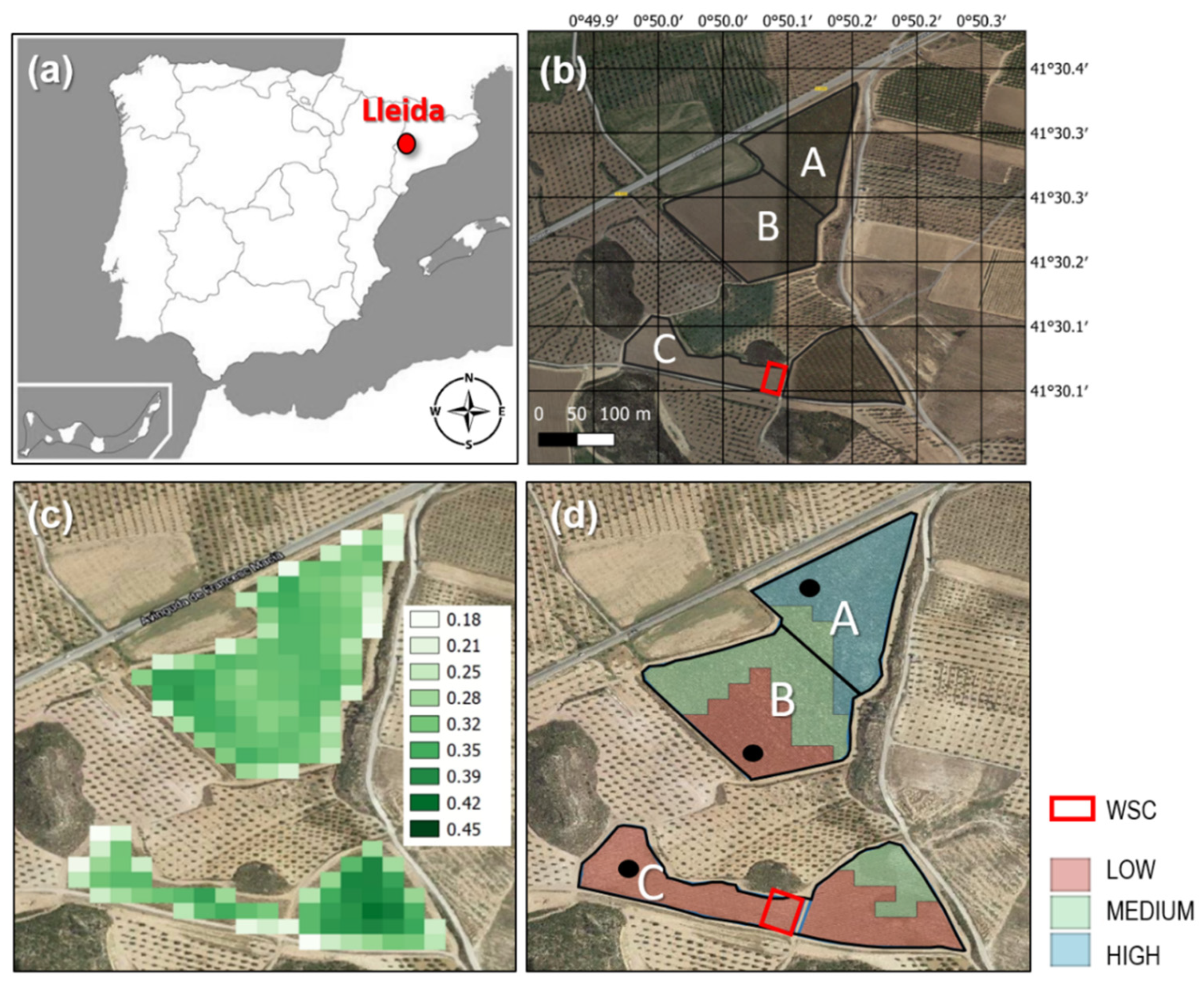
2.1. Study Site

This study was carried out during the growing seasons 2020 and 2021 in a 6.9 ha commercial vineyard (cv. Grenache) located in Aranyó (41°30′18″ N–0°50′09″ E, 316 m, Lleida, Spain) (Figure 1). The vineyard comprised three different irrigation sectors of 2.0, 2.3 and 2.6 ha (Figure 1b). Vines were planted in 2018 with a 110 Rister rootstock and at 1.0 × 2.0 m spacing distance. Two irrigation sectors (A and B) were oriented at 140 ° (NW-SE), while irrigation sector C was oriented at 100 ° (close to E-W). The canopy system was trained using vertical shoot positioning (VSP), with a bilateral, spur-pruner cordon located 0.7 m above the ground. Soil was left bare throughout the growing season. Irrigation was provided by means of a single pipe with drippers every 1 m, whose nominal flow was 2 L/h. Disease control and nutrition vine management were conducted by Family Torres winery following the organic wine grape production protocol of the ‘Costers del Segre’ Denomination of Origin (Catalonia, Spain). The area has a typical Mediterranean climate, with dry and hot summers and mild winters. Total annual rainfall in 2020 and 2021 was 475 and 288 mm, respectively. The annual reference evapotranspiration (ET0) for each year was 1071 and 1065 mm, respectively.
In addition, an area of 0.2 ha within irrigation sector C was used to evaluate the soil water balance simulations obtained by the digital twin and to compare the simulated evapotranspiration and stem water potential with, respectively, the remote sensing estimations of evapotranspiration and stem water potential measurements (Figure 1b). In this area, water stress cycles (WSC) were conducted throughout both studied growing seasons. This area contained two pure pixels of 20 m. The WSC consisted of cutting irrigation for short periods of time, twice per campaign, until measured stem water potential (Ψstem) reached values below −1.2 MPa and then recovering vine water status again.
During 2020, irrigation scheduling was conducted by the winegrower without using the cloud-based irrigation decision support system described in Section 2.3. In that year, data were only gathered and used for simulations and validations. During 2021, irrigation scheduling was carried out through the automated irrigation DSS. The DSS assimilated in near real time information of remotely sensed estimates of daily fiPAR and data from soil moisture sensors and weather stations in order to calculate vine water requirements.

2.2. Selection of the Location for Installing Sensors

Sentinel-2 fAPAR time series were analyzed during the 2019 growing season [39]. A more detailed explanation of the approach used to estimate fAPAR with Sentinel-2 is explained later in the manuscript (Section 2.5). The averaged seasonal fAPAR of 2019 was used to classify different management zones within the vineyard based on vegetative growth (Figure 1c). Three different zones corresponding to different canopy vigor levels (Low, Medium and High) were identified using the k-means clustering tool (QGIS software, version Hannover 3.16) (Figure 1d). In each irrigation sector, a representative measuring point was selected taking into account the fAPAR classification map. The point was placed in the zone with the highest percentage within each irrigation sector. This representative point within each irrigation sector was visually selected to install the soil moisture sensors at different positions. For each point, soil properties were also analyzed and soil moisture release curves obtained by Hyprop 2 (METER Group, Pullman, WA, USA) (Table 1).
Three soil moisture sensors (TEROS-10, METER Group, Pullman, WA, USA) were installed in each representative point at 0.3 m depth at three different positions: below the emitter, and at 0.25 m and 0.5 m from the emitter. An MTKD water meter (LabFerrer S.L., Cervera, Lleida, Spain) was also installed in each point to measure the amount of water applied and to monitor irrigation events. All sensors were connected to a ZL6 datalogger (METER Group, Pullman, WA, USA) via cables, and the data stored at a 15-min frequency at the ZENTRA cloud platform in near real time. Meteorological data were automatically gathered from the website of the Meteorological Service of Catalonia (SMC, www.ruralcat.net/web/guest/agrometeo.estacions) corresponding to a weather station (Les Borges Blanques) located 1.5 km from the vineyard.

2.3. IrriDesk® and Definition of the Irrigation Seasonal Plan

The automated irrigation decision support system (DSS) used in this study, so called IrriDesk®, is open-access accessible for research purposes through a non-commercial version and also commercially available to any grower through an external company. IrriDesk® (www.irridesk.com) is a cloud-hosted platform developed under the paradigm of digital twin, which on a daily basis, sends updated prescriptions to irrigation controllers, following the integration of different data sources such as local sensors, meteorological and remote sensing data. IrriDesk® is an evolution of IRRIX, which has previously been used in several trials of sensor-based irrigation control [21,23,24]. In both cases, the underlying approach for irrigation scheduling is a site-specific soil water balance (SWB) fine-tuned by sensors [22]. In this approach, irrigation prescriptions for each management zone are calculated once a day, based on an SWB model, in mm/day, and are sent machine-to-machine to the irrigation controller after conversion to minutes of irrigation per irrigation event, considering the properties of the irrigation system and the programmed irrigation frequency.
A relevant feature of IrriDesk® is that irrigation scheduling is guided by a seasonal plan, which allows the application of more elaborate strategies, such as supplemental irrigation and RDI for managing irrigation with limiting water allocations. The seasonal plan specifies, for each day, a range of acceptable accumulated irrigation since the start of the season until that day. Then, if the measured irrigation approaches the borders of that range (maximum and minimum), the irrigation prescriptions do not respond to sensors but are calculated to keep the accumulated irrigation within the range. The target soil moisture is also specified in the seasonal plan and can be set at different values along the season. Additionally, intended water unbalances can be specified at precise periods of the season in terms of the ratio between the irrigation to prescribe and the irrigation resulting from the SWB model.
In the trials reported in this study, the seasonal plan was elaborated through SWB simulations, using as inputs the agronomical description of the crop, soil and irrigation setup, the historical weather at the site in the previous 10 years, the range of annual irrigation applied in previous years and the curve of intended water unbalance agreed between researchers and farmer. In the studied vineyard, the upper and lower applied water thresholds were, respectively, set at 150 and 230 mm (Figure 2c). Since the aim was to adopt an RDI strategy, water status levels were defined as a multiplier of irrigation needs or intended water deviations from the SWB (Figure 2a). For instance, in this study the multiplier was set to 0.6 during pre-veraison because the winegrower wanted to stress vines at this phenological stage. Immediately before veraison, the multiplier was set to 1.5 in order to recover vine water status. During post-veraison, it progressively decreased from 1.0 to 0.7. During post-harvest, water status was recovered again by defining a threshold of 1.0. Based on these values, the relative soil water content upper and lower limits were also adjusted throughout the growing season (Figure 2b). All these curves were predefined to determine admissible bounds for the irrigation scheduling and to ensure that irrigation inputs above those available for the campaign were not used.
At the beginning of the growing season, the DSS considered an expected seasonal curve of daily fIPARd based on the values measured the previous year. As the season progressed, new observed values were obtained from remote sensing. The new values of estimated fIPARd at the observation day were assimilated as the weighted average between observed and expected values, where the weights were set at 0.9 and 0.1, respectively. The expected values for the remaining part of the season were also modified. In general, the expected fIPARd values were re-scaled to fit the new value with the expected value. However, in early and late stages of the growing season, when fIPARd was expected to undergo rapid variations with either shooting or leaf fall, the time axis was modified to fit the new with the expected value.
With the configuration set in these trials, the daily irrigation dose (did) (mm/day) were calculated as:
did =   iwu ET 0   fKx fIPAR d + Ke   effRain + SPcorrection
where iwu is the intended water unbalance specified in the seasonal plan, ET0 is the reference evapotranspiration measured the previous day at a nearby weather station (mm/day), fKx is an empirically adjusted coefficient from feedback by soil moisture sensors [22], fIPARd is the expected fIPARd for that day (%), obtained from S2 fAPAR and upscaled on a daily time step with Oyarzun’s model, Ke is the coefficient for soil evaporation [3] calculated by the model, effRain is the effective rain of the previous day (mm), obtained from pluviometer measurements and recalculated by the model, and SPcorrection is the required addition or subtraction of irrigation to keep the measurements within the range specified in the seasonal plan.
In addition to scheduling irrigation, the digital twin behind IrriDesk® models the different variables of the soil water balance. The SWB model is based on the rationale of AquaCrop [55] plus specific adaptations to deal with discontinuous canopies and drip irrigation. For instance, it deals with daily fIPAR and soil water content is obtained by individually simulating nine compartments spatially distributed throughout the tree spacing (three blocks with three soil profile layers in depth). The simulated SWB variables were used to calculate the Crop Water Stress Index (CWSI) as one minus the ratio between actual and potential transpiration rate (1 − Ta/Tp) [56].

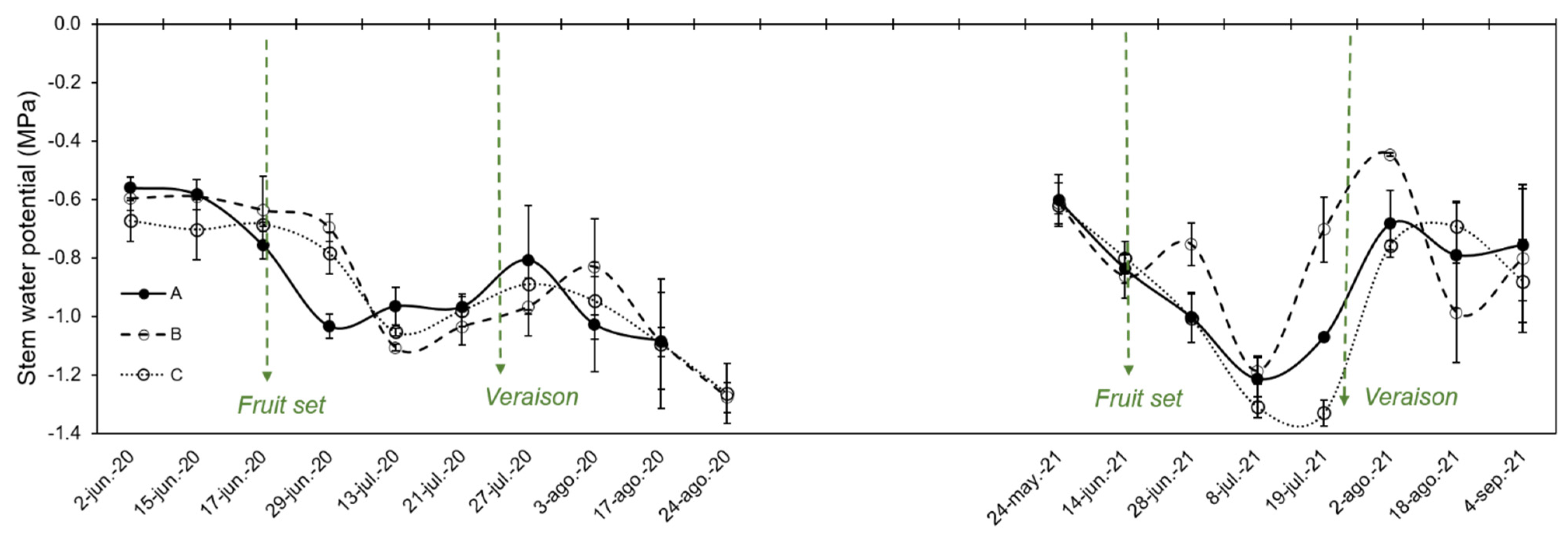
2.4. Field Measurements

Ψstem was measured in each representative point throughout the 2020 and 2021 growing seasons every two weeks at noon with a pressure chamber (model 3005; Soil Moisture Equipment Corp. Santa Barbara, CA, USA) following the protocol described by McCutchan and Shackel [57]. Shaded leaves were wrapped in plastic bags covered with aluminum foil at least one hour before Ψstem measurements. All measurements were taken in less than one hour with three leaves at each point, one in each single vine.
On the other hand, fIPAR was measured from 11:00 to 13:00 h (GMT+2) using a portable ceptometer (AccuPAR Linear PAR, Decagon Devices, Inc., Pullman, WA, USA) on the same dates as Ψstem. Incident PAR above and below vines was measured in five vines in a row per point. Measurements were conducted in horizontal position at ground level and perpendicular to vine row. In order to cover vine spacing, five equally spaced measurements were determined in an open space adjacent to each vine. Vine structural parameters such as height and canopy width perpendicular to the row were also measured on each occasion. These data were used to calculate fIPARd through the hourly Oyarzun model [54] and further used to validate remote sensing fAPAR. The canopy porosity parameter of Oyarzun’s model was adjusted so that the instantaneous measured value of fIPAR agreed with the simulated value.

2.5. Satellite Imagery and Biophysical Variables

Multispectral instruments on Sentinel-2A and Sentinel-2B satellites provide high resolution multispectral shortwave observations of Earth’s surface with a geometric revisit time at the equator of 5 days [58]. S2 overpass through the study site was between 10:36 and 10:50 GTM. S2 images at level-2A were downloaded for the study site from Copernicus Open Access hub (https://scihub.copernicus.eu/ (last accessed on 15 November 2022)) using the Sentinelsat library (https://sentinelsat.readthedocs.io/en/stable/ (last accessed on 15 November 2022)). Biophysical variables of the vegetation were estimated from the S2 biophysical processor [39] available in the SNAP software v8.0 (https://step.esa.int/main/download/snap-download/, last accessed on 11 December 2021). This processor relies on building a randomized dataset of vegetation biophysical variables from which reflectance simulations by the radiative transfer models (RTM) PROSPECT and SAIL are produced [59]. Therefore, instantaneous values of biophysical variables were obtained at the time of the satellite overpass for those days under clear sky conditions. In total, 23 and 22 S2 images were processed from April to October for 2020 and 2021, respectively. fAPAR was empirically regressed with both instantaneous and daily modeled fiPAR (fIPARd). Then, each time a S2 image was available, fAPAR of each irrigation sector was converted to fIPARd and assimilated into the digital twin to calculate grapevine water requirements (Equation (1)). In addition, the leaf area index (LAI) and the fractional vegetation cover (FVC) were used to derive actual evapotranspiration with the TSEB-PT model.

2.6. Actual and Potential Evapotranspiration Using Copernicus-Based Inputs

Sentinel-3A and Sentinel-3B images from the sea and land surface radiometer (SLSTR) were downloaded to obtain LST at 1 km resolution. In total, 99 and 111 cloud-free S3 images were processed in 2020 and 2021 for the same period mentioned for S2. The DMS approach [49] was used, combining S2 and S3 images to sharpen 1 km coarse spatial resolution LST from S3 to 20 m. The methodology used is described by Guzinski et al. [50]. Meteorological inputs were obtained from the European Center of Medium Weather Forecast (ECMWF) ERA5 reanalysis dataset [60]. This dataset has a 30 km grid and was used to run the TSEB-PT model. For the current study, the variables used were air temperature at 2 m, dew point temperature at 2 m, wind speed at 100 m, surface pressure and total column water vapor (TCWV). In addition, aerosol optical thickness (AOT) at 550 m was obtained from the Copernicus Atmosphere Monitoring Service (CAMS) since it is not included in ERA5. Two ancillary sources of data were also used: land cover maps from the Copernicus Climate Change Service (C3S) (https://cds.climate.copernicus.eu/cdsapp#!/dataset/satellite-land-cover?tab=overview, last accessed on 10 October 2021) and the digital elevation model (DEM) of the shuttle radar topography mission (SRTM). In the study site, the C3S landcover map, produced at 300 m resolution, did not vary from one year to another, and so the one from 2017 was used for both years. A look-up table of different parameters associated to each crop class was set up in accordance with Guzinski et al. [50].
The TSEB-PT modeling approach [61] estimates the energy fluxes of both soil and canopy, separately based on a single bulk LST measurement that initially assumes a maximum potential rate of transpiration. This first guess, which usually starts with an alpha coefficient of 1.26, is sequentially reduced until realistic fluxes are obtained [62]. This model has been used to derive land-surface energy fluxes using Copernicus-based inputs (TSEB-PTS2+S3) [50,51,52,53]. Further details on the TSEB model scheme can be found at the source code (https://github.com/hectornieto/pyTSEB., last accessed on 22 April 2022) and the original formulation of the model [42].
On the other hand, potential evapotranspiration (ETp), defined as the water usage (or evapotranspiration rate) of a well-watered crop was computed from the Penman–Monteith model, assuming a maximum stomatal conductance [63,64]. ETp was therefore computed using S2 LAI estimations and the same meteorological inputs as in the TSEB-PTS2+S3. For both cases, instantaneous energy fluxes at the satellite overpass were upscaled to daily water fluxes, expressed in units of mm/day, by multiplying the instantaneous ratio of latent heat fluxes over solar irradiance by the average daily solar irradiance [65]. Gap filling was applied following the protocol described by Jofre-Cekalović et al. [53]. Both TSEB-PTS2+S3 and the Penman–Monteith estimated ET were intercompared with that modelled through the digital twin by computing their correlation as well as their root mean square deviation ( RMSD = ( x i y i ) 2 N ). The RMSD is analogous to the root mean square error (RMSE), but denotes deviations between two independent estimates (x and y) rather than the error from one estimate to a reference measurement.

3. Results and Discussion

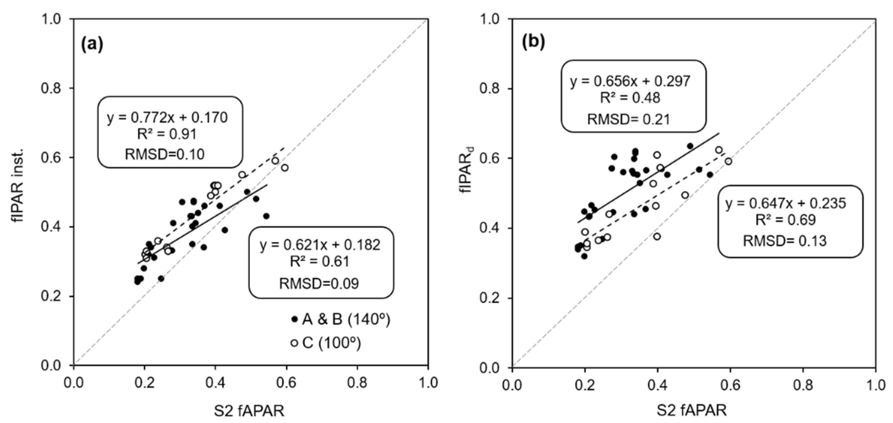
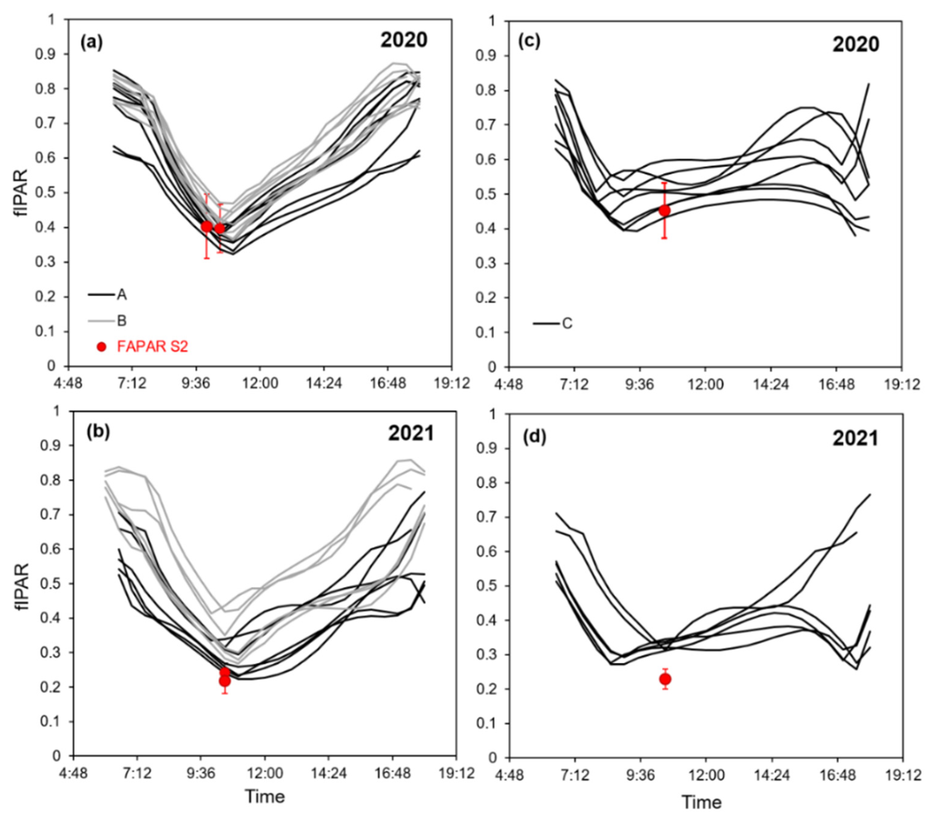
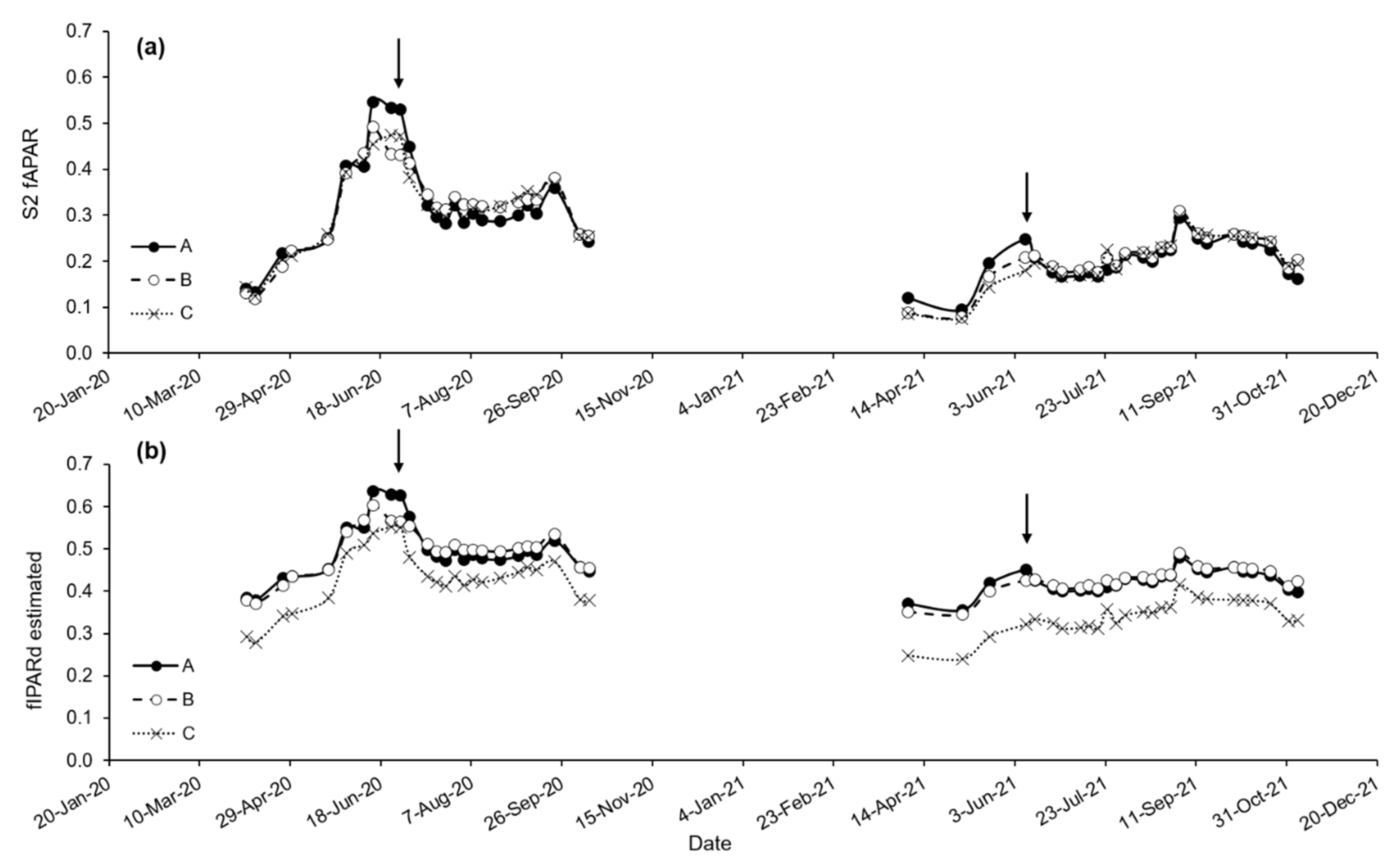
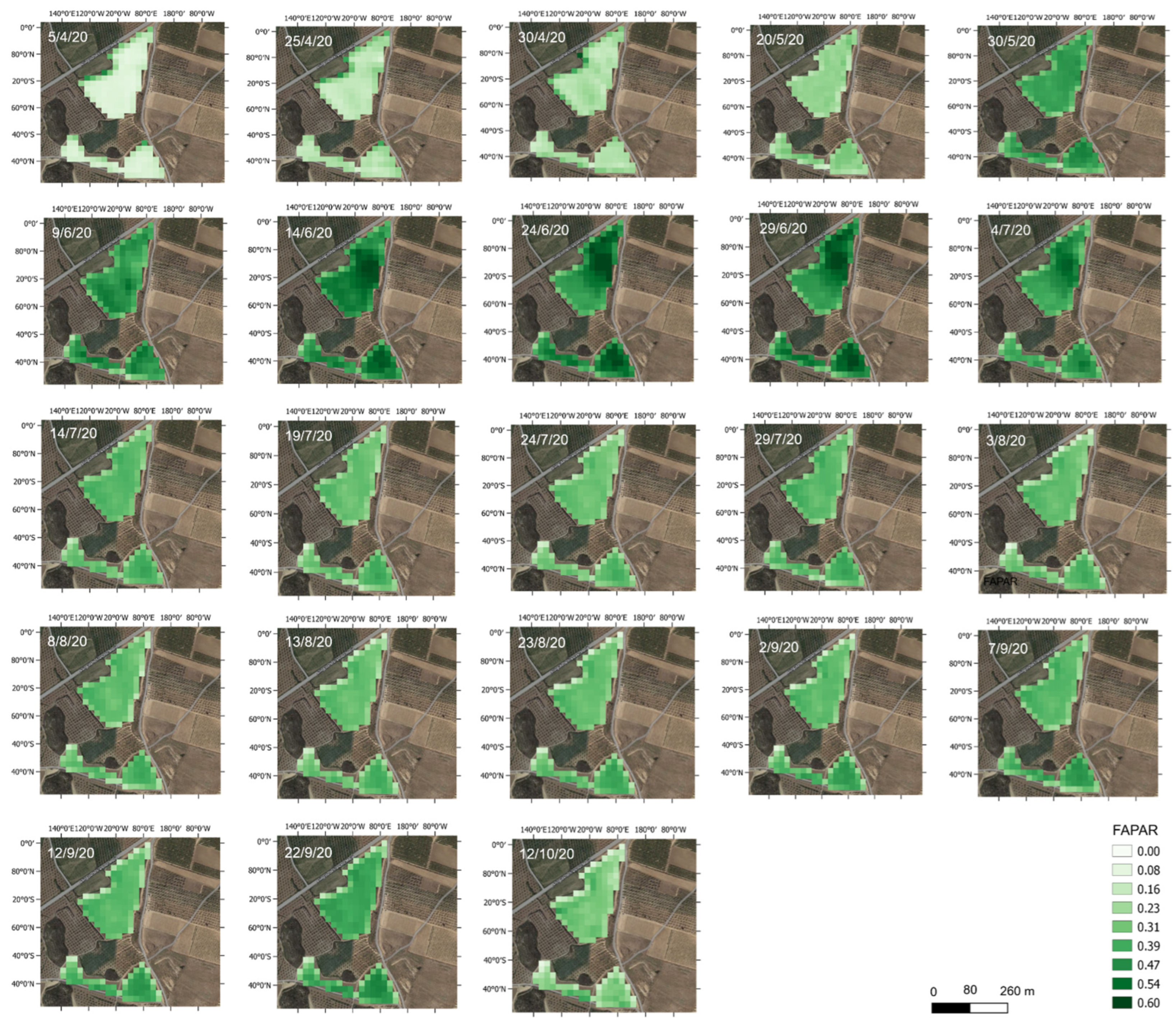
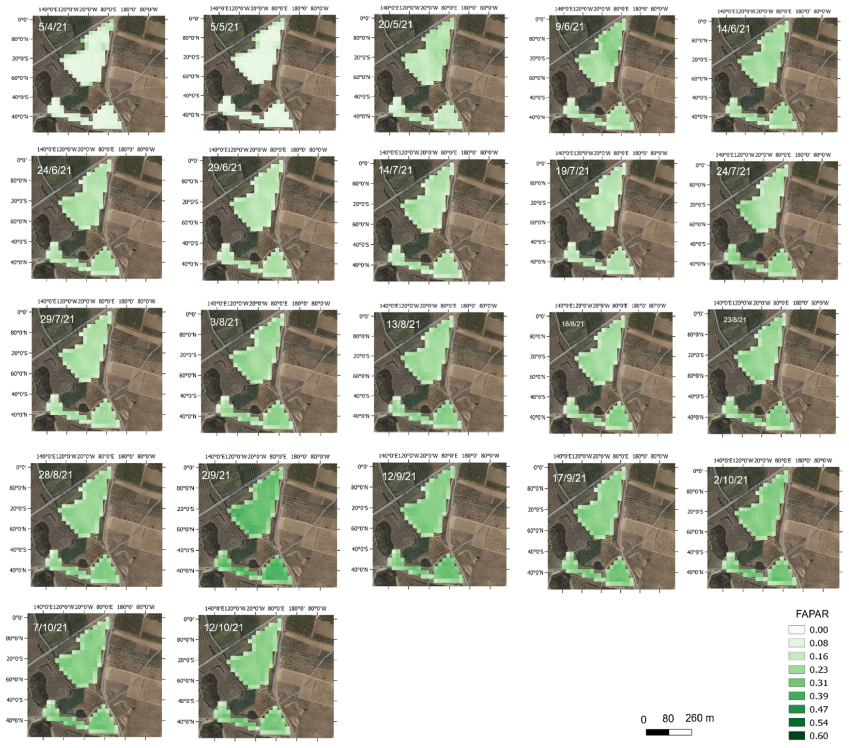
3.1. Sentinel-2 fAPAR

S2 fAPAR was compared with fIPAR under the hypothesis that for green canopies the latter is a good proxy of fAPAR. This assumption is valid mostly during the non-senescence periods of the growing season due to the strong absorption capacity in this spectral domain of the photosynthetic pigments [66] and the usually small background reflectivities for well-developed canopies [40,41,67]. A comparison of instantaneous S2 fAPAR with in situ measurements of fIPAR at the same time as the satellite overpassed showed an R2 of 0.61 and 0.91 for irrigation sectors with 140° and 100° row orientation, respectively (Figure 3a). These coefficients of determination are quite promising and suggest the suitability of using S2 fAPAR in discontinuous canopies, particularly in conditions without cover crop in the interrow. On the other hand, the existence of cover crop in the interrow could be a problem when estimating the biophysical parameters of the canopy, especially with the spatial resolutions provided by the current open-source satellites. The RMSD, which ranged from 0.09 to 0.10 indicated that this relationship did not significantly vary between row orientations. This deviation, however, may be explained by soil background reflectance and diffuse illumination variations due to multiscattering or also due to the poor representativeness of five vines within a 20 m pixel. Wojnowski et al. [68] reported that fIPAR is typically 6–9% higher than fAPAR. Despite this, the deviation obtained is insignificant for the purposes of this study.
Since most growth simulation models, including the one used in this study, have a daily time step, instantaneous S2 fAPAR was regressed with the modelled daily fIPAR (fIPARd) obtained from Oyarzun’s model. This regression showed differences between row orientation (Figure 3b). In both irrigation sectors, fIPARd tended to be higher than instantaneous S2 fAPAR. In addition, irrigation sectors with rows oriented closer to a N-S direction (closer to 180°) had a higher fIPARd than others. As mentioned, the modelled fiPARd was computed with Oyarzun’s modelling approach [54], which is based on geometric relationships between the stand structure, the sun’s position, and the length of the shadow cast by the trees. Some studies have indicated that the instantaneous fAPAR value at 10:00 solar time is very close to the daily integrated value under clear sky conditions [69]. However, it was found in this study that, particularly in discontinuous woody crops planted in rows and sometimes with different training systems, this is not always the case and that it varies with row orientation. Figure 4 shows the diurnal trends of hourly modelled fIPAR in each irrigation sector and the estimated instantaneous S2 fAPAR for 2020 and 2021. Each line corresponds to a different date. Results indicate that irrigation sectors A and B (140° row orientation) tend to intercept more light throughout the day than C. As rows of A and B are closest to an N-S orientation, the model follows an expected hourly symmetrical path with respect to near solar noon with higher fractional interception in the early morning and late afternoon, and a minimum at approximately midday. On the other hand, the fIPAR of irrigation sector C (100° row orientation) was more constant throughout the day, except for early morning and late afternoon. The S2 satellite overpass, and therefore fAPAR estimates, coincide with the minimum daily values of fIPAR for rows oriented at 140° (Figure 4a,b). The same agreement was observed for irrigation sector C in 2020 (Figure 4c). However, it seems that for irrigation sector C in 2021 the S2 fAPAR was slightly lower in comparison to the modelled fIPAR at the time of satellite overpass. A possible explanation, which needs to be corroborated in further studies, may be related to a higher soil background effect in the rows oriented at 100° due to the vines having lower canopy vigor in 2021 than in 2020.
The seasonal distribution of S2 fAPAR showed differences between growing seasons (Figure 5a). Overall, fAPAR in 2020 was higher than in 2021. This is explained by a rainier spring in 2020. In both years, fAPAR increased during the spring until reaching maximum values in approximately mid-June. These maximum fAPAR values were 0.55 and 0.24 in 2020 and 2021, respectively. Consequently, a summer pruning was carried out at mid-June which significantly reduced vegetative growth. Differences in fAPAR between irrigation sectors were only observed just before summer pruning, with irrigation sector A having the highest fAPAR. During 2021, instantaneous S2 fAPAR was converted to fIPARd using the empirical regression obtained in Figure 3b and consequently assimilated in the digital twin in order to calculate vine water requirements. Figure 5b shows the seasonal evolution of estimated fIPARd. It can be observed that irrigation sectors A and B have a higher fIPARd than C throughout both growing seasons. Spatio-temporal time series of S2 fAPAR also illustrate these patterns during both growing seasons (Appendix A).

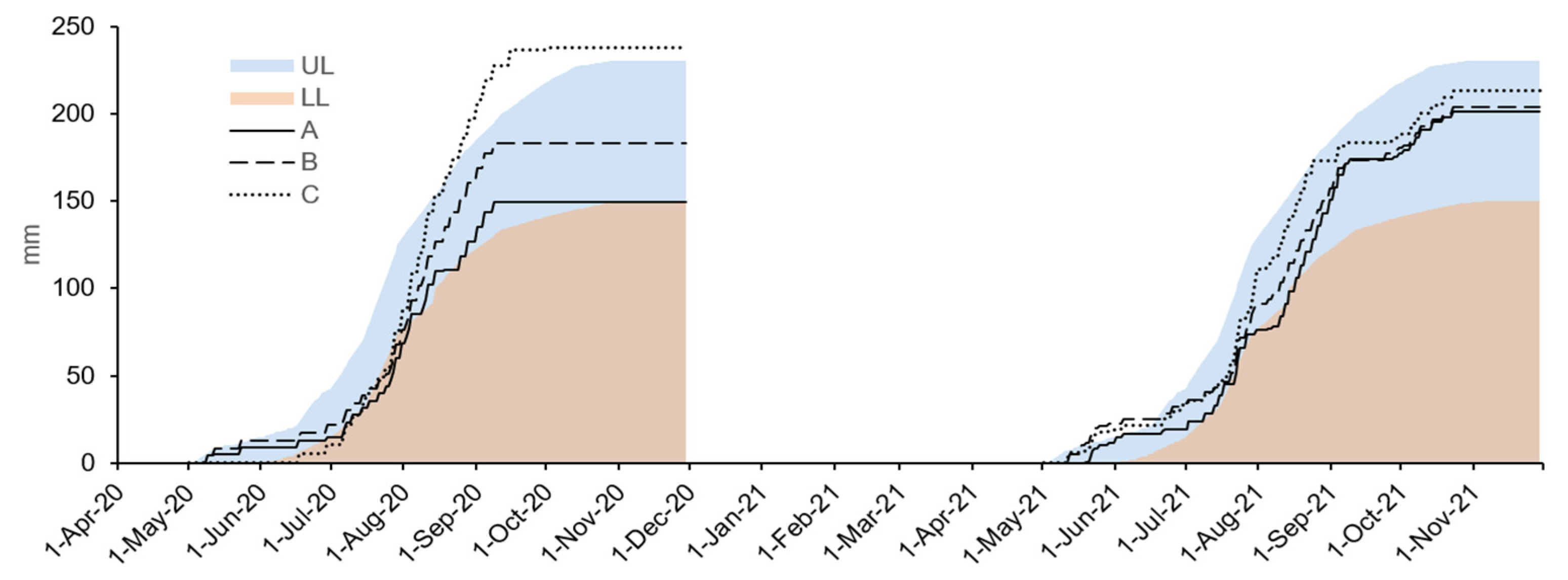
3.2. Performance of the Automated Decision Support System for Irrigation Scheduling

The performance of the DSS in terms of the automated scheduling of irrigation of a vineyard during 2021 was compared with the traditional irrigation management that the winegrower conducted in 2020. In the latter, the winegrower clearly applied different amounts of water in each irrigation sector (Figure 6). The total amount of water applied was 150, 183 and 238 mm in A, B and C, respectively. In contrast, the amounts of water applied in 2021 were always between the maximum and minimum thresholds predefined at the beginning of the growing season. The total amount of water applied in 2021 was 201, 235 and 213 mm for A, B and C, respectively. The spatial variability of this vineyard is not particularly high, which explains why the differences in the amount of applied water were insignificant.
Data recorded with soil moisture sensors located at different positions detected both irrigation and precipitation events throughout the growing season (Figure 7). Irrigation events were more noticeable and had a quicker response in soil moisture sensors located at 0 and 25 cm from the emitter than those at 50 cm. Sensor-to-sensor variability has been widely analyzed and can be attributed to the small volume of soil measured, sensor sensitivity to local variations in soil properties or the spatial and dynamic heterogeneity in wet bulbs around emitters [21,23,70,71,72]. Although some studies have recommended installing sensors at different depths and positions, to install a large number of sensors for commercially scheduled irrigation is very expensive. Domínguez-Niño et al. [72] analyzed soil moisture positioning according to soil water dynamics and concluded that, in the context of SWB-based automated irrigation scheduling fine-tuned with soil moisture sensors, the recommended sensor locations can be a combination of sensors close to the vertical of the dripper and other sensors midway between neighboring drippers, at 30 cm depth. In our study, we positioned the soil moisture sensors following this recommendation.
It can be observed in the soil moisture data corresponding to 2020 that the winegrower did not irrigate in any sector from fruit-set to veraison (Figure 7a,c,e). As a consequence, soil moisture decreased. Irrigation events occurred again during post-veraison in order to recover vine water status. Comparing this strategy with Ψstem values measured in each irrigation sector, it can be observed that the winegrower was able to stress vines during pre-veraison to Ψstem values of −1.1 MPa (Figure 8). However, although the vines recovered slightly at veraison, the Ψstem values subsequently dropped again until harvest. This suggests that despite applying large amounts of water during post-veraison, this was nevertheless insufficient to recover vine water status until the end of the growing season. A different irrigation strategy was conducted in 2021, following the seasonal plan predefined and based on intentional water balance deviation and a range of cumulative irrigation thresholds (Figure 2a). Soil moisture sensors indicated high soil moisture values for all irrigation sectors at the beginning of the growing season due to spring precipitations and the first irrigation events during May. These large amounts of applied irrigation water were higher than the predefined cumulative irrigation thresholds, so irrigation was automatically stopped for some dates (Figure 6). This fact also coincided with the lowest multiplier of water needs (0.6) during fruit-set, which was maintained throughout the month of June. Consequently, the seasonal plan defined in the DSS comprised starting vine water status recovery from early July in order to reach veraison with vines transpiring at near potential rates. Accordingly, the DSS started triggering irrigation again by the end of June. Irrigation in sector C started, however, some days before A and B because soil water moisture in C was lower. Despite these first irrigation events at the end of June, Ψstem values continued falling for some days (Figure 8). An improvement in Ψstem was only observed in sector B on one measurement day, but the values fell again on the next measurement day. The minimum Ψstem value of −1.2 MPa for irrigation sectors A and B was reached on 8 July 2021, while for irrigation sector C lower values were reached and lasted longer. This can be explained as the result of the soil depth in C being lower and, therefore, also the available soil water content explored by the rooting system. Because the relative soil water content was below the pre-established thresholds only a few days before veraison, the DSS automatically prescribed more water. It can be observed how, after these irrigation events, the trend in daily minimum values of soil moisture increased a few days before veraison in A and B but not as much in C (Figure 7b,d,f). It was at veraison, and after large water irrigation amounts, that soil moisture in C reached values close to field capacity (Figure 7f). Figure 9 also shows how Ψstem in A and B recovered earlier than in C at veraison. During post-veraison, the irrigation strategy consisted of nearly meeting vine water requirements. In contrast to 2020, Ψstem values remained constant at values between −0.8 and −1.0 MPa until harvest.
Overall, this study demonstrates the feasibility of scheduling irrigation through an automated SWB approach fine-tuned with capacitance-type soil moisture sensors and the assimilation of remote sensing estimates of biophysical parameters. Here, we observed how the adaptive response allowed spontaneous adjustments in order to stress vines to a certain level at specific growing stages.

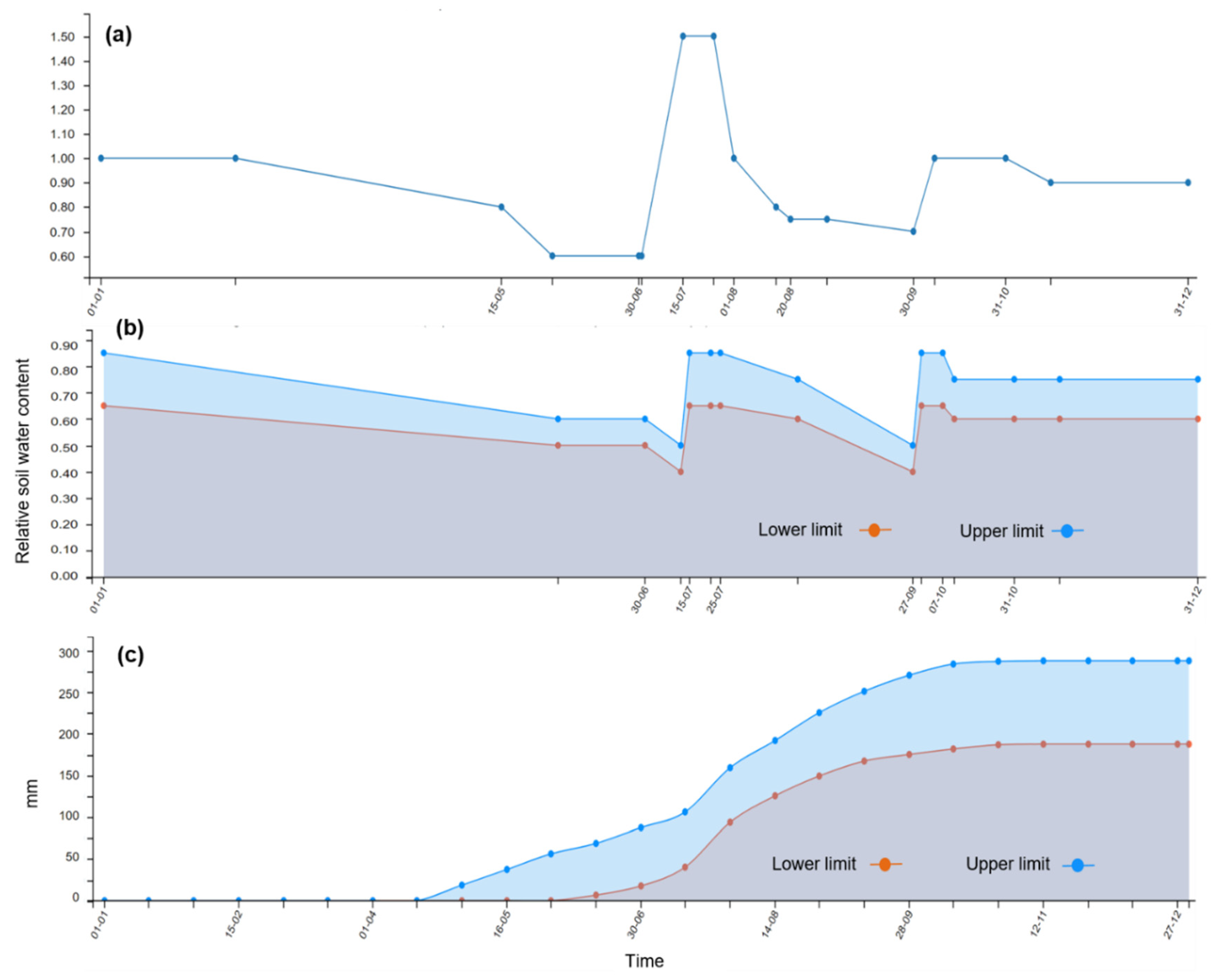
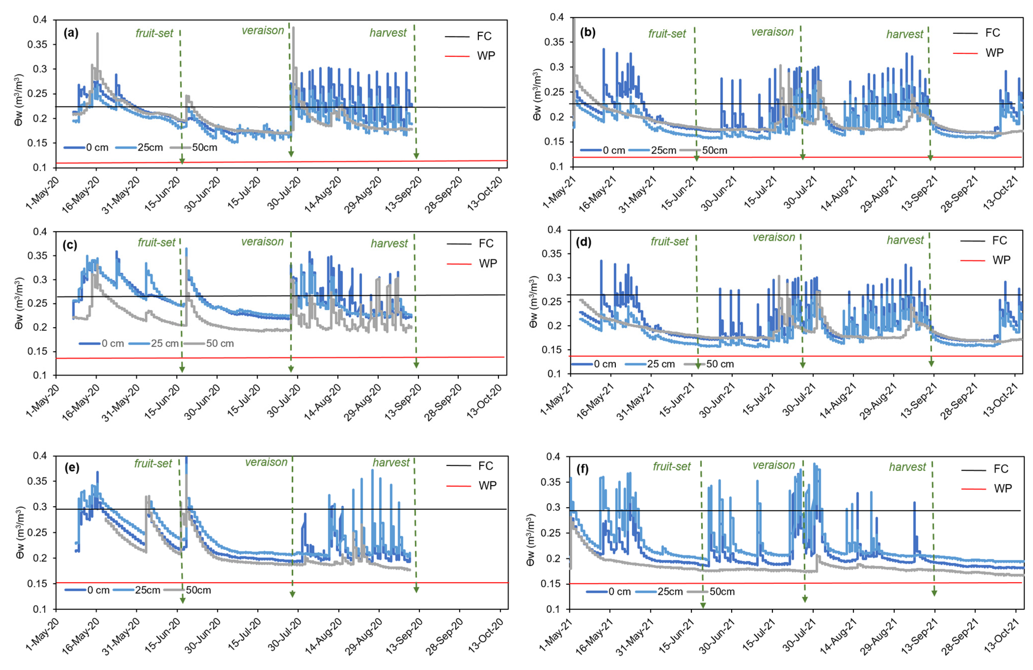
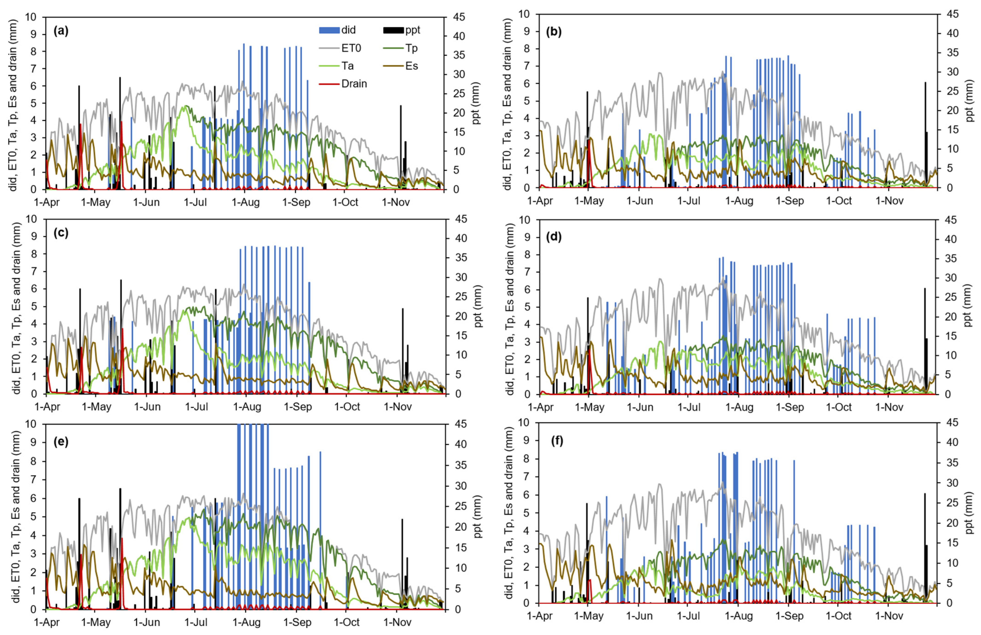
3.3. Simulations of the Water Balance Variables through the Digital Twin

Table 2 shows a summary of the total cumulative values of modelled evapotranspiration, water use efficiency and water stress. Rainfall in 2020 was greater than in 2021. As already seen in the fAPAR values shown in Figure 5, this caused greater vine vegetative growth and, consequently, greater vine water demand. For this reason, both ETp and ETa values of 2020 were higher than in 2021. With regard to the (rain + irrigation)/ETp ratio, vines received slightly less water in relation to its needs in 2020, when irrigation was carried out at the farmer’s discretion. In 2021, irrigation sector B received the highest percentage of water applied in relation to its needs, which may explain the higher Ψstem values observed in some specific moments. Except for irrigation sector C, the ETa/ETp ratio was lower in 2020 than in 2021, suggesting that vines were more stressed in the second year. Figure 9 shows the simulations of the SWB variables in each irrigation sector throughout the 2020 and 2021 growing seasons. Potential transpiration (Tp) was higher in 2020 than in 2021. Actual transpiration (Ta) was similar to Tp until late June, but once RDI was adopted Ta began to fall below Tp. During this period, Ta was approximately 49% and 45% lower than Tp for 2020 and 2021, respectively. In 2021, irrigation sector C was more stressed than sectors A and B, with cumulative Ta approximately 64% lower than Tp. This concurs with the lowest Ψstem observed during pre-veraison. After each precipitation event, a peak can be observed corresponding to drainage and soil evaporation. Soil evaporation peaks after each irrigation event can also be observed. In total, the vineyard’s average soil evaporation represented 41% and 54% of total ETa for 2020 and 2021, respectively (Table 2). Although there was more rainfall in 2020, soil evaporation increased in 2021 because the number of days with irrigation events was higher. These percentages of soil evaporation throughout the growing season are not far from values reported in the literature, which vary from 22 to 59% ETa depending on the amount of rainfall and irrigation events [73,74,75].

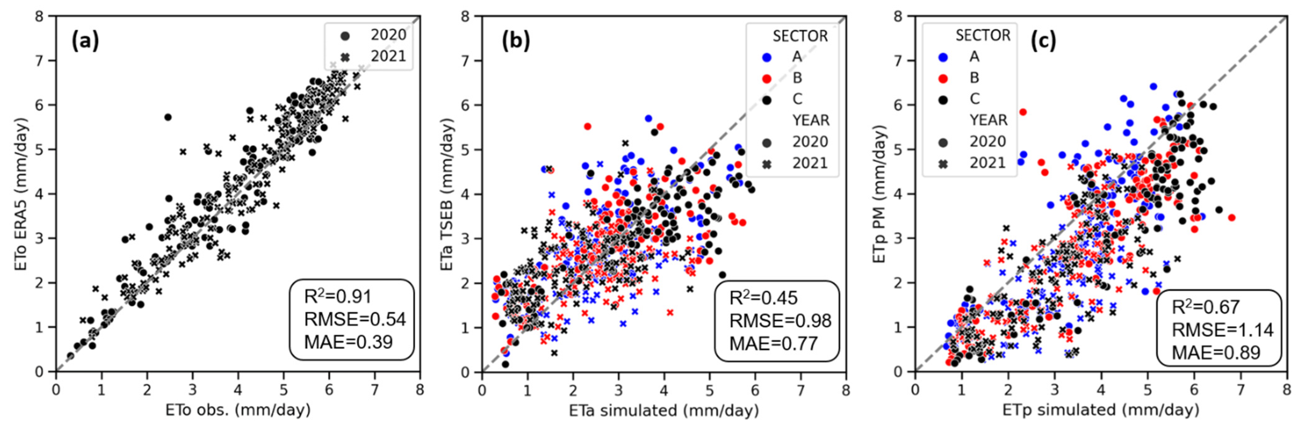
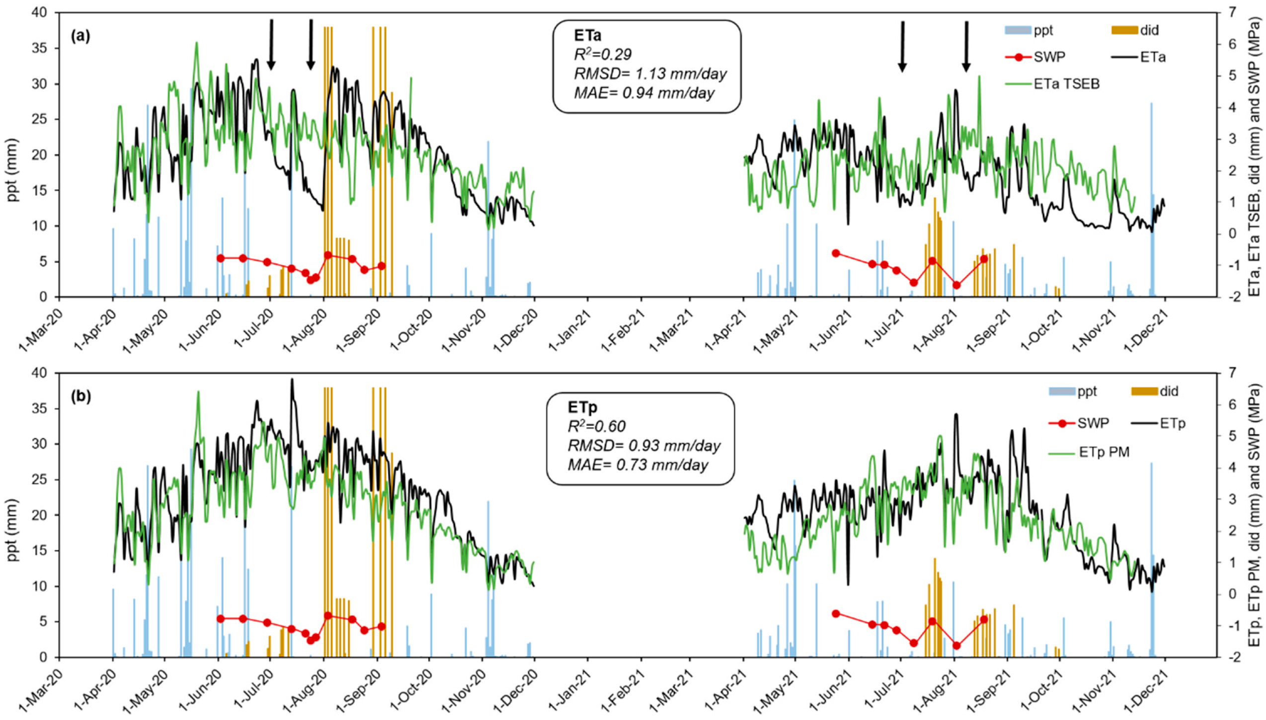
3.4. Comparison of Digital Twin Simulations of ET with Values Estimated with Remote Sensing

In this study, we did not have the opportunity to install a flux tower or sap flow sensors to validate the simulations of evapotranspiration or the plant water status made through the digital twin in each of the irrigation sectors of the vineyard. Instead, we used stem water potential (Ψstem) as an indicator of plant water status and compared ET simulations with the values estimated through remote sensing using SEB modelling approaches.
The crop water stress index (CWSI) [56] was correlated with Ψstem (Figure 10). By using the empirical equation, it is possible to obtain the thresholds of Ψstem for a CWSI of zero and one, which, respectively, corresponded to −0.51 MPa and −2.3 MPa. These thresholds seem reasonable and concur with those reported in similar studies [76].
A previous step to compare ET between different approaches was to discard the possibility of the use of meteorological data from different sources affecting ET estimations. Figure 11a shows how the daily reference ET0 obtained from ERA5 correlated with that obtained from the closest weather station to the vineyard. The RMSD was 0.54 mm/day, thus ruling out the influence of meteorological data on the error metrics observed in ETa and ETp estimates. The regression between modelled and estimated ETa using two years of data showed an RMSD of 0.98 mm/day (Figure 11b) with a coefficient of regression of 0.45. The R2 and RMSD for ETp were 0.67 and 1.14 mm/day, respectively (Figure 11c). An ANOVA analysis was conducted to assess differences in the RMSD of both ETa and ETp between years and irrigation sectors, but the results were not statistically significant. Although numerous studies have demonstrated the potential of using TSEB-PT to monitor ETa, very few have validated the TSEB-PT using Copernicus-based inputs. Studies validated with flux towers concluded that the RMSE of instantaneous heat flux was approximately 30% in agricultural areas [50,53]. Guzinski et al. [51] also obtained an RMSE of 0.96 mm/day when validation was performed for multiple crops together, including irrigated and rainfed. In addition, it is known from previous studies that TSEB-PT is quite sensitive to a correct determination of canopy structure/roughness [51,77]. Therefore, any error in the parameters assigned in the lookup table associated to land cover maps or in the estimates of biophysical variables could yield larger uncertainties in ETa estimates with the TSEB-PTS2+S3 approach. Another source of bias could be the inability of the DMS approach to capture precise values of LST when crops are under short-term water stress and there is no evidence of a decrease in biomass [52,53]. Therefore, since the vineyard of this study was under water stress for some periods, it cannot be ruled out that ETa estimates with the TSEB-PTS2+S3 approach were overestimated for some dates in comparison to the simulation with the SWB approach. This hypothesis is further validated in a small part of the vineyard where short water stress cycles were adopted and vine water status monitored throughout the growing season (Figure 12). Figure 11 also shows that both remotely sensed ETa and ETp were underestimated for many dates. This could be attributable to the different methodologies used to assimilate the biophysical parameters. The remote sensing SEB approach uses instantaneous estimates of S2 LAI as an input in order to iteratively derive fIPAR through the Campbell and Norman technique [78]. This is then used to derive instantaneous energy fluxes, which are later upscaled to daily fluxes considering the average daily solar irradiance [65]. In contrast, the SWB approach used by the irrigation DSS assimilates fIPARd, which was derived from S2 fAPAR and upscaled to a daily time step through Oyarzun’s model. Because this hypothesis is speculative, further studies should be conducted in order to validate the simulations of the different SWB parameters obtained through IrriDesk’s digital twin.

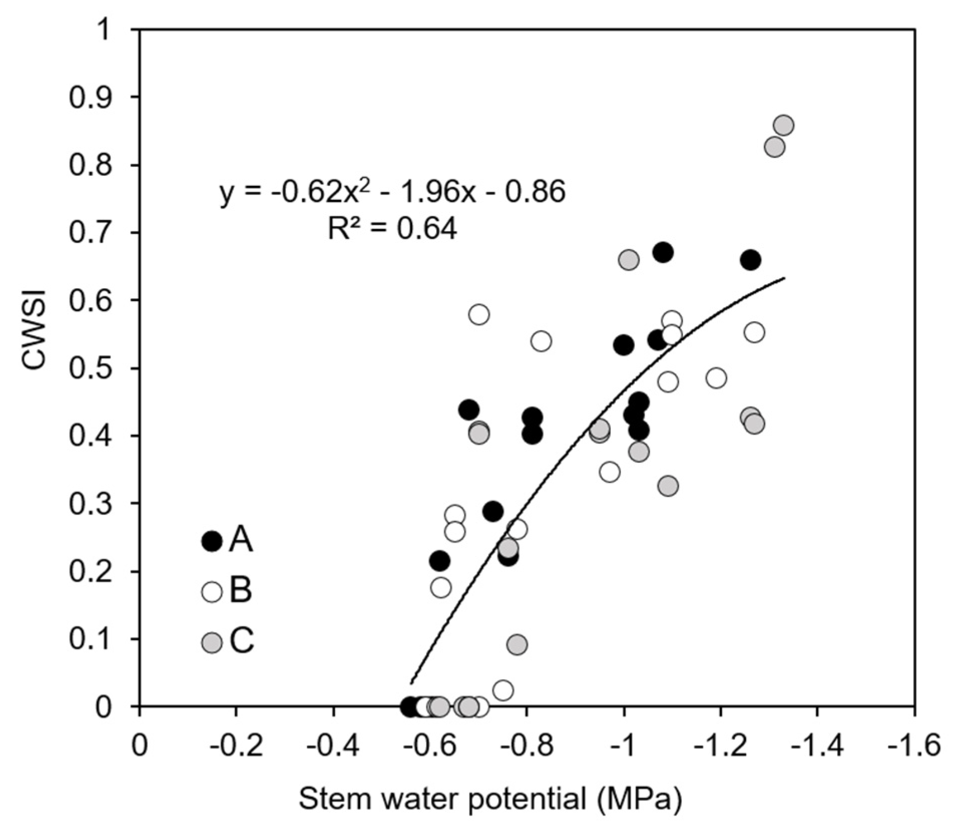
3.5. Comparison of the Response of ET in Vines under Water Stress Cycles (WSC)

Seasonal variation in Ψstem shows the periods when water stress occurred, twice in each growing season (Figure 12). Irrigation was stopped for short periods of time until measured Ψstem reached severe water stress values. On each occasion, vine water status was recovered again by applying large amounts of water. Minimum Ψstem values were −1.46 and −1.60 MPa for 2020 and 2021, respectively. Both ETa and ETp followed the same trend throughout both growing seasons, with higher rates in 2020 than in 2021 due to the higher vegetative growth in the first year. The R2 and RMSD between the digital twin simulations and remotely sensed estimates of ETp and ETa, were, respectively, 0.60 and 0.93 mm/day and 0.29 and 1.13 mm/day. For ETp, the regression seems reasonable and the deviation was mostly due to an underestimation in remotely sensed ETp. The possible reason for this has previously described in this paper. On the other hand, this analysis confirms the hypothesis that the TSEB-PTS2+S3 tends to overestimate evapotranspiration when water stress occurs for short periods of time. This can be observed in the periods when Ψstem values were more negative. In those periods, while simulated ETa decreases, the ETa TSEB-PTS2+S3 remains high with values close to ETp. The cause of this is based on the inability of the DMS approach to capture the full range of surface temperatures [52]. Since sharpened LST was obtained from machine learning algorithms which relate S3 LST with S2 shortwave bands at coarse resolutions, it is probable that differences in sharpened LST can mainly be attributed to differences in vegetative growth variables, but not when short-term water stress occurs and the amount of biomass is not reduced [53].

4. Conclusions and Perspective

This study tested the feasibility of scheduling irrigation through an automated soil water balance (SWB) approach fine-tuned with capacitance-type soil moisture sensors and pre-defined irrigation amount thresholds. Results show that estimates of grapevine fAPAR from Sentinel-2 had a RMSD of 0.10 in comparison with in situ measurements of instantaneous fIPAR, independently of row orientation. Modelled fIPARd was between 13% and 21% higher than instantaneous S2 fAPAR, and dependent on row orientation. Vineyards with rows oriented close to 140° had a higher fIPARd than those oriented at 100°. This suggests that crop growth models that need a daily time step of light interception as an input and intend to assimilate remote sensing estimates of biophysical variables should consider that S2 fAPAR corresponds to instantaneous values. Therefore, models such as Oyarzun’s can be a successful alternative to upscale from instantaneous to daytime scale, and considering row orientation. Using the DSS in 2021, this study demonstrated the feasibility of calculating vine water requirements and the automated scheduling of irrigation by assimilating in near real time estimates of fIPARd.
The DSS also demonstrated its suitability to automatically carry out an RDI strategy by applying different amounts of water in different irrigation sectors. Simulations of soil water balance components through the digital twin seem to perform well. For instance, differences in both simulated ETa and ETp were observed between years, attributable to higher vine vegetative growth in 2020 than in 2021. In addition, simulated Ta decreased up to 49% in comparison to Tp when water stress was adopted following an RDI strategy, and simulated CWSI (as 1 − Ta/Tp) was correlated with Ψstem. Simulations of ETa and ETp showed RMSD values of 0.98 and 1.14 mm/day, respectively, when compared with estimations obtained from remote sensing surface energy balance models. To obtain accurate spatio-temporal estimations of crop water status in water stress conditions continues to be an enormous challenge. Although this study demonstrates the capacity of the digital twin to obtain accurate simulations of vine water status under different levels of water stress, and to schedule the irrigation of individual irrigation sectors on this assumption, it is important to highlight that these simulations were obtained using soil moisture sensor data from a single representative vine. This study shows, once again, the current difficulty in estimating and monitoring water stress in heterogeneous row crops using satellite remote sensing approaches due to the lack of a high spatio-temporal resolution thermal sensor. Some studies have validated the TSEB-PTS2+S3 approach in multiple crops, obtaining an averaged RMSE of 0.96 mm/day [51]. However, the water stress cycles experiment conducted in this study shows that when vines were under short periods of water stress and there was no evidence of a decrease in biomass, the disaggregation methodology used to downscale land surface temperature (LST) was not able to estimate high values of LST and therefore ETa was overestimated in comparison with the SWB-simulated ETa.

Author Contributions

Conceptualization, J.B., M.T. and J.C.; methodology, J.B., A.P., M.P.-S. and J.C.; resources, J.B., A.P., M.P.-S., J.V., M.T. and J.C.; supervision, J.B. and J.C.; writing—original draft, J.B. and J.C.; writing—review and editing, J.B., A.P., M.P.-S., J.V., M.T. and J.C. All authors have read and agreed to the published version of the manuscript.

Funding

This research was funded by the projects IRRINTEGRAL (No. RTI2018-099949-R-C21) and DIGISPAC (No. TED2021-131237B-C21), both from the Ministry of Science, Innovation and Universities of the Spanish government.

Data Availability Statement

Not applicable.

Acknowledgments

The authors would like to thank all the Efficient Use of Water in Agriculture program team at the IRTA for their technical support, as well as Family Torres winery. This study was undertaken as part of the Horizon 2020 Programme for Research and Innovation (H2020) of the European Commission, in the context of the Marie Sklodowska-Curie Research and Innovation Staff Exchange (RISE) action and ACCWA project: grant agreement No.: 823965.

Conflicts of Interest

The authors declare no conflict of interest.

Appendix A

Figure A1. Maps of fAPAR derived from the Sentinel-2 biophysical processor, showing the spatio-temporal variation throughout the 2020 growing season.
Water 15 02506 g0a1
Figure A2. Maps of fAPAR derived from the Sentinel-2 biophysical processor, showing the spatio-temporal variation throughout the 2021 growing season.
Water 15 02506 g0a2

References

  1. Calzadilla, A.; Rehdanz, K.; Tol, R.S.J. The GTAP-W Model: Accounting for Water Use in Agriculture; Kiel Working Paper, 2011, No. 1745; Kiel Institute for the World Economy (IfW): Kiel, Germany, 2011; Available online: http://hdl.handle.net/10419/54939 (accessed on 20 February 2023).
  2. ISPA. 2020. Available online: https://www.ispag.org/about/definition (accessed on 21 October 2022).
  3. Allen, R.G.; Pereira, L.S.; Raes, D.; Smith, M. Crop evapotranspiration—Guidelines for computing crop water requirements. In FAO Irrigation and Drainage; Paper No. 56; Food and Agriculture Organization: Rome, Italy, 1998. [Google Scholar]
  4. Intrieri, C.; Poni, S.; Rebucci, B.; Magnanini, E. Row orientation effects on whole-canopy gas exchange of potted and field-grown grapevines. Vitis 1998, 37, 147–154. [Google Scholar] [CrossRef]
  5. Marsal, J.; Johnson, S.; Casadesus, J.; Lopez, G.; Girona, J.; Stöckle, C. Fraction of canopy intercepted radiation relates differently with crop coefficient depending on the season and the fruit tree species. Agric. For. Meteorol. 2014, 184, 1–11. [Google Scholar] [CrossRef]
  6. Ayars, J.E.; Johnson, R.S.; Phene, C.J.; Trout, T.J.; Clark, D.A.; Mead, R.M. Water use by drip-irrigated late-season peaches. Irrig. Sci. 2003, 22, 187–194. [Google Scholar] [CrossRef]
  7. Auzmendi, I.; Mata, M.; del Campo, J.; Lopez, G.; Girona, J.; Marsal, J. Intercepted radiation by apple canopy can be used as a basis for irrigation scheduling. Agric. Water Manag. 2011, 98, 886–892. [Google Scholar] [CrossRef]
  8. Girona, J.; del Campo, J.; Mata, M.; Lopez, G.; Marsal, J. A comparative study of apple and pear tree water consumption measured with two weighing lysimeters. Irrig. Sci. 2011, 29, 55–63. [Google Scholar] [CrossRef]
  9. Egea, G.; Nortes, P.A.; González-Real, M.M.; Baille, A.; Domingo, R. Agronomic response and water productivity of almond trees under contrasted deficit irrigation regimes. Agric. Water Manag. 2010, 97, 171–181. [Google Scholar] [CrossRef]
  10. Memmi, H.; Gijón, M.C.; Couceiro, J.F.; Pérez-López, D. Water stress thresholds for regulated deficit irrigation in pistachio trees: Rootstock influence and effects on yield quality. Agric. Water Manag. 2016, 164, 58–72. [Google Scholar] [CrossRef] [Green Version]
  11. Moñino, M.J.; Blanco-Cipollone, F.; Vivas, A.; Bodelón, O.G.; Prieto, M.H. Evaluation of different deficit irrigation strategies in the late-maturing Japanese plum cultivar ‘Angeleno’. Agric. Water Manag. 2020, 234, 106111. [Google Scholar] [CrossRef]
  12. Intrigliolo, D.; Castel, J.R. Response of plum trees to deficit irrigation under two crop levels: Tree growth, yield and fruit quality. Irrig. Sci. 2010, 28, 525–534. [Google Scholar] [CrossRef]
  13. Basile, B.; Marsal, J.; Mata, M.; Vallverdú, X.; Bellvert, J.; Girona, J. Phenological Sensitivity of Cabernet Sauvignon to Water Stress: Vine Physiology and Berry Composition. Am. J. Enol. Vitic. 2011, 62, 452–461. [Google Scholar] [CrossRef] [Green Version]
  14. Lipan, L.; Martín-Palomo, M.J.; Sánchez-Rodríguez, L.; Cano-Lamadrid, M.; Sendra, E.; Hernández, F.; Burló, F.; Vázquez-Araújo, L.; Andreu, L.; Carbonell-Barrachina, A.A. Almond fruit quality can be improved by means of deficit irrigation strategies. Agric. Water Manag. 2019, 217, 236–242. [Google Scholar] [CrossRef]
  15. Jones, H.G. Irrigation scheduling: Advantages and pitfalls of plant-based methods. J. Exp. Bot. 2004, 55, 2427–2436. [Google Scholar] [CrossRef] [Green Version]
  16. Goldhamer, D.A.; Fereres, E. Irrigation scheduling of almond trees with trunk diameter sensors. Irrig. Sci. 2004, 23, 11–19. [Google Scholar] [CrossRef]
  17. Dukes, M.D.; Zotarelli, L.; Morgan, K.T. Use of irrigation technologies for vegetable crops in Florida. HortTechnology 2010, 20, 133–142. [Google Scholar] [CrossRef] [Green Version]
  18. Soulis, K.X.; Elmaloglou, S.; Dercas, N. Investigating the effects of soil moisture sensors positioning and accuracy on soil moisture based drip irrigation scheduling Systems. Agric. Water Manag. 2015, 148, 258–268. [Google Scholar] [CrossRef]
  19. Osroosh, Y.; Peters, R.T.; Campbell, C.S.; Zhang, Q. Comparison of Irrigation Automation Algorithms for Drip-Irrigated Apple Trees. Comput. Electron. Agric. 2016, 128, 87–99. [Google Scholar] [CrossRef] [Green Version]
  20. Dukes, M.D.; Scholberg, J.M. Soil moisture controlled subsurface drip irrigation on sandy soils. Appl. Eng. Agric. 2005, 21, 89–101. [Google Scholar] [CrossRef]
  21. Millán, S.; Campillo, C.; Casadesús, J.; Pérez-Rodríguez, J.M.; Prieto, M.H. Automatic irrigation scheduling on a hedgerow olive orchard using an algorithm of water balance readjusted with soil moisture sensors. Sensors 2020, 20, 2526. [Google Scholar] [CrossRef]
  22. Casadesús, J.; Mata, M.; Marsal, J.; Girona, J. A general algorithm for automated scheduling of drip irrigation in tree crops. Comput. Electron. Agric. 2012, 83, 11–20. [Google Scholar] [CrossRef]
  23. Domínguez-Niño, J.M.; Oliver-Manera, J.; Girona, J.; Casadesús, J. Differential irrigation scheduling by an automated algorithm of water balance tuned by capacitance- type soil moisture sensors. Agric. Water Manag. 2020, 228, 105880. [Google Scholar] [CrossRef]
  24. Millán, S.; Casadesús, J.; Campillo, C.; Moñino, M.J.; Prieto, M.H. Using Soil Moisture Sensors for Automated Irrigation Scheduling in a Plum Crop. Water 2019, 11, 2061. [Google Scholar] [CrossRef] [Green Version]
  25. Grieves, M. Digital Twin: Manufacturing Excellence through Virtual Factory Replication. Florida Institute of Technology. Digit. Twin White Pap. 2014, 1, 1–7. [Google Scholar]
  26. ESA. Sentinel-2 User Handbook; ESA Standard Document, Issue 1, Rev. 2.; ESA: Peris, France, 2015; Available online: www.copernicus.eu (accessed on 15 May 2022).
  27. Bausch, W.C.; Neale, C.M.U. Crop coefficients derived from reflected canopy radiation: A concept. Trans. ASAE 1987, 30, 703–709. [Google Scholar] [CrossRef]
  28. Campos, I.; Neale, C.M.U.; Calera, A.; Balbontín, C.; González-Piqueras, J. Assessing satellite-based basal crop coefficients for irrigated grapes (Vitis vinífera L.). Agric. Water Manag. 2010, 98, 45–54. [Google Scholar] [CrossRef]
  29. Kamble, B.; Kilic, A.; Hubbard, K. Estimating Crop Coefficients Using Remote Sensing-Based Vegetation Index. Remote Sens. 2013, 5, 1588–1602. [Google Scholar] [CrossRef] [Green Version]
  30. Haboudane, D.; Miller, J.R.; Pattey, E.; Zarco-tejada, P.J.; Strachan, I.B. Hyperspectral vegetation indices and novel algorithms for predicting green LAI of crop canopies: Modeling and validation in the context of precision agriculture. Remote Sens. Environ. 2004, 90, 337–352. [Google Scholar] [CrossRef]
  31. Delalieux, S.; Somers, B.; Hereijgers, S.; Verstraeten, W.W.; Keulemans, W.; Coppin, P. A near-infrared narrow-waveband ratio to determine Leaf Area Index in orchards. Remote Sens. Environ. 2008, 112, 3762–3772. [Google Scholar] [CrossRef]
  32. Hall, F.G.; Huemmrich, K.F.; Goetz, S.J.; Sellers, P.J.; Nickerson, J.E. Satellite remote sensing of surface energy balance, failures, and unresolved issues in FIFE. J. Geophys. Res. 1992, 97, 19061–19089. [Google Scholar] [CrossRef]
  33. Myneni, R.B.; Williams, D.L. On the relationship between FAPAR and NDVI. Remote Sens. Environ. 1994, 49, 200–211. [Google Scholar] [CrossRef]
  34. Leolini, L.; Moriondo, M.; Rossi, R.; Bellini, E.; Brilli, L.; López-Bernal, Á.; Santos, J.A.; Fraga, H.; Bindi, M.; Dibari, C.; et al. Use of Sentinel-2 Derived Vegetation Indices for Estimating fPAR in Olive Groves. Agronomy 2022, 12, 1540. [Google Scholar] [CrossRef]
  35. Leolini, L.; Bregaglio, S.; Ginaldi, F.; Costafreda-Aumedes, S.; Di Gennaro, S.F.; Matese, A.; Maselli, F.; Caruso, G.; Palai, G.; Bajocco, S.; et al. Use of remote sensing-derived fPAR data in a grapevine simulation model for estimating vine biomass accumulation and yield variability at sub-field level. Precis. Agric. 2022, 24, 705–726. [Google Scholar] [CrossRef]
  36. Huete, A.R. Soil influences in remotely sensed vegetation-canopy spectra. In Theory and Application of Optical Remote Sensing; Asrar, G., Ed.; Wiley Series in Remote Sensing; Wiley: New York, NY, USA, 1989; pp. 107–141. [Google Scholar]
  37. Kempeneers, P.; Zarco-Tejada, P.J.; North, P.R.J.; De Backer, S.; Delalieux, S.; Sepulcre-Cantó, G.; Morales, F.; Van Aardt, J.A.N.; Sagardoy, R.; Coppin, P.; et al. Model inversion for chlorophyll estimation in open canopies from hyperspectral imagery. Int. J. Remote Sens. 2008, 29, 5093–5111. [Google Scholar] [CrossRef]
  38. Guillén-Climent, M.L.; Zarco-Tejada, P.J.; Villabobos, F.J. Estimating radiation interception in an olive orchard using physical models and multispectral airborne imagery. Isr. J. Plant Sci. 2012, 60, 107–121. [Google Scholar] [CrossRef] [Green Version]
  39. Weiss, M.; Baret, F. S2ToolBox Level 2 Products: LAI, FAPAR, FCOVER—Version 1.1. Sentinel2 ToolBox Level2 Products; INRA: Paris, France, 2016; pp. 1–53. Available online: https://step.esa.int/docs/extra/ATBD_S2ToolBox_L2B_V1.1.pdf (accessed on 19 August 2022).
  40. Gower, S.T.; Kucharik, C.J.; Norman, J.M. Direct and Indirect Estimation of Leaf Area Index, fAPAR, and Net Primary Production of Terrestrial Ecosystems. Remote Sens. Environ. 1999, 70, 29–51. [Google Scholar] [CrossRef]
  41. Li, W.; Fang, H.; Wei, S.; Weiss, M.; Baret, F. Critical analysis of methods to estimate the fraction of absorbed or intercepted photosynthetically active radiation from ground measurements: Application to rice crops. Agric. For. Meteorol. 2021, 297, 108273. [Google Scholar] [CrossRef]
  42. Norman, J.M.; Kustas, W.; Humes, K. A two-source approach for estimating soil and vegetation energy fluxes from observations of directional radiometric surface temperature. Agric. For. Meteorol. 1995, 77, 263–293. [Google Scholar] [CrossRef]
  43. Bastiaanssen, W.G.M.; Menenti, M.; Feddes, R.A.; Holtslag, A.A.M. A remote sensing surface energy balance algorithm for land (SEBAL). 1. Formulation. J. Hydrol. 1998, 212–213, 198–212. [Google Scholar] [CrossRef]
  44. Allen, R.G.; Tasumi, M.; Trezza, R. Satellite-based energy balance for mapping evapotranspiration with internalized calibration (METRIC)—Model. J. Irrig. Drain. Eng.-Asce 2007, 133, 380–394. [Google Scholar] [CrossRef]
  45. Merlin, O.; Duchemin, B.; Hagolle, O.; Jacob, F.; Coudert, B.; Chehbouni, G.; Dedieu, G.; Garatuza, J.; Kerr, Y. Disaggregation of MODIS surface temperature over an agricultural area using a time series of Formosat-2 images. Remote Sens. Environ. 2010, 114, 2500–2512. [Google Scholar] [CrossRef] [Green Version]
  46. Agam, N.; Kustas, W.P.; Anderson, M.C.; Li, F.; Neale, C.M. A vegetation index based technique for spatial sharpening of thermal imagery. Remote Sens. Environ. 2007, 107, 545–558. [Google Scholar] [CrossRef]
  47. Zhou, J.; Liu, S.; Li, M.; Zhan, W.; Xu, Z.; Xu, T. Quantification of the Scale Effect in Downscaling Remotely Sensed Land Surface Temperature. Remote Sens. 2016, 8, 975. [Google Scholar] [CrossRef] [Green Version]
  48. Bisquert, M.; Sánchez, J.M.; Caselles, V. Evaluation of Disaggregation Methods for Downscaling MODIS Land Surface Temperature to Landsat Spatial Resolution in Barrax Test Site. IEEE J. Sel. Top. Appl. Earth Obs. Remote Sens. 2016, 9, 1430–1438. [Google Scholar] [CrossRef] [Green Version]
  49. Gao, F.; Kustas, W.P.; Anderson, M.C. A data mining approach for sharpening thermal satellite imagery over land. Remote Sens. 2012, 4, 3287–3319. [Google Scholar] [CrossRef] [Green Version]
  50. Guzinski, R.; Nieto, H.; Sandholt, I.; Karamitilios, G. Modelling High-Resolution Actual Evapotranspiration through Sentinel-2 and Sentinel-3 Data Fusion. Remote Sens. 2020, 12, 1433. [Google Scholar] [CrossRef]
  51. Guzinski, R.; Nieto, H.; Sánchez, J.M.; López-Urrea, R.; Boujnah, D.M.; Boulet, G. Utility of Copernicus-Based Inputs for Actual Evapotranspiration Modeling in Support of Sustainable Water Use in Agriculture. IEEE J. Sel. Top. Appl. Earth Obs. Remote Sens. 2021, 14, 11466–11484. [Google Scholar] [CrossRef]
  52. Bellvert, J.; Jofre-Čekalović, C.; Pelechá, A.; Mata, M.; Nieto, H. Feasibility of Using the Two-Source Energy Balance Model (TSEB) with Sentinel-2 and Sentinel-3 Images to Analyze the Spatio-Temporal Variability of Vine Water Status in a Vineyard. Remote Sens. 2020, 12, 2299. [Google Scholar] [CrossRef]
  53. Jofre-Čekalović, C.; Nieto, H.; Girona, J.; Pamies-Sans, M.; Bellvert, J. Accounting for Almond Crop Water Use under Different Irrigation Regimes with a Two-Source Energy Balance Model and Copernicus-Based Inputs. Remote Sens. 2022, 14, 2106. [Google Scholar] [CrossRef]
  54. Oyarzun, R.A.; Stöckle, C.O.; Whiting, M.D. A simple approach to modeling radiation interception by fruit-tree orchards. Agric. For. Meteorol. 2007, 142, 12–24. [Google Scholar] [CrossRef]
  55. Steduto, P.; Raes, D.; Theodore Hsiao, C.; Fereres, E.; Heng, L.K.; Hower, T.A.; Evett, S.R.; RojasLara, B.A.; Farahani, H.J.; Izzi, G.; et al. Concepts and Applications of AquaCrop: The FAO Crop Water Productivity Model. In Crop Modelling and Decision Support; Cao, W., White, J.W., Wang, E., Eds.; Springer: Berlin/Heidelberg, Germany, 2009; pp. 175–191. [Google Scholar] [CrossRef] [Green Version]
  56. Jackson, R.D.; Idso, S.B.; Reginato, R.J.; Pinter, P.J., Jr. Canopy temperature as a crop water stress indicator. Water Resour. Res. 1981, 17, 1133–1138. [Google Scholar] [CrossRef]
  57. McCutchan, H.; Shackel, K.A. Stem water potential as a sensitive indicator of water stress in prune trees (Prunus domestica L. cv French). J. Am. Soc. Hortic. Sci. 1992, 117, 607–611. [Google Scholar] [CrossRef] [Green Version]
  58. Drusch, M.; Del Bello, U.; Carlier, S.; Colin, O.; Fernandez, V.; Gascon, F.; Hoersch, B.; Isola, C.; Laberinti, P.; Martimort, P.; et al. Sentinel-2: ESA’s optical high-resolution mission for GMES operational services. Remote Sens. Environ. 2012, 120, 25–36. [Google Scholar] [CrossRef]
  59. Jacquemoud, S.; Verhoef, W.; Baret, F.; Bacour, C.; Zarco-Tejada, P.J.; Asner, G.P.; François, C.; Ustin, S.L. PROSPECT+SAIL models: A review of use for vegetation characterization. Remote Sens. Environ. 2009, 113, S56–S66. [Google Scholar] [CrossRef]
  60. Hersbach, H.; Bell, B.; Berrisford, P.; Hirahara, S.; Horányi, A.; Muñoz-Sabater, J.; Nicolas, J.; Peubey, C.; Radu, R.; Schepers, D.; et al. The ERA5 global reanalysis. Q. J. R. Meteorol. Soc. 2020, 146, 1999–2049. [Google Scholar] [CrossRef]
  61. Kustas, W.P.; Nieto, H.; Morillas, L.; Anderson, M.C.; Alfieri, J.G.; Hipps, L.E.; Villagarcía, L.; Domingo, F.; Garcia, M. Revisiting the paper “Using radiometric surface temperature for surface energy flux estimation in Mediterranean drylands from a two-source perspective”. Remote Sens. Environ. 2016, 184, 645–653. [Google Scholar] [CrossRef] [Green Version]
  62. Priestley, C.H.B.; Taylor, R.J. On the Assessment of Surface Heat Flux and Evaporation Using Large-Scale Parameters. Mon. Weather Rev. 1972, 100, 81–92. [Google Scholar] [CrossRef]
  63. Monteith, J.L.; Unsworth, M.H. Chapter 13: Steady state heat balance. In Principles of Environmental Physics, 3rd ed.; Academic Press: Burlington, VT, USA, 2008; pp. 250–255. [Google Scholar]
  64. Allen, R.G.; Pruitt, W.O.; Wright, J.L.; Howell, T.A.; Ventura, F.; Snyder, R.; Itenfisu, D.; Steduto, P.; Berengena, J.; Yrisarry, J.B.; et al. A recommendation on standardized surface resistance for hourly calculation of reference ET0 by the FAO56 Penman-Monteith method. Agric. Water Manag. 2006, 81, 1–22. [Google Scholar] [CrossRef]
  65. Cammalleri, C.; Anderson, M.C.; Kustas, W.P. Upscaling of evapotranspiration fluxes from instantaneous to daytime scales for thermal remote sensing applications. Hydrol. Earth Syst. Sci. 2014, 18, 1885–1894. [Google Scholar] [CrossRef] [Green Version]
  66. Andrieu, B.; Baret, F. Indirect methods of estimating crop structure from optical measurements. In Crop Structure and Light Microclimate—Characterization and Applications; Varlet-Grancher, R.B.C., Sinoquet, H., Eds.; INRA: Paris, France, 1993; pp. 285–322. [Google Scholar]
  67. Li, W.; Weiss, M.; Waldner, F.; Defourny, P.; Demarez, V.; Morin, D.; Hagolle, O.; Baret, F. A Generic Algorithm to Estimate LAI, FAPAR and FCOVER Variables from SPOT4_HRVIR and Landsat Sensors: Evaluation of the Consistency and Comparison with Ground Measurements. Remote Sens. 2015, 7, 15494–15516. [Google Scholar] [CrossRef] [Green Version]
  68. Wojnowski, W.; Wei, S.; Li, W.; Yin, T.; Li, X.-X.; Ow, G.L.F.; Mohd Yusof, M.L.; Whittle, A.J. Comparison of Absorbed and Intercepted Fractions of PAR for Individual Trees Based on Radiative Transfer Model Simulations. Remote Sens. 2021, 13, 1069. [Google Scholar] [CrossRef]
  69. Baret, F.; Hagolle, O.; Geiger, B.; Bicheron, P.; Miras, B.; Huc, M.; Berthelot, B.; Niño, F.; Weiss, M.; Samain, O.; et al. LAI, fAPAR and fCover CYCLOPES global products derived from VEGETATION: Part 1: Principles of the algorithm. Remote Sens. Environ. 2007, 110, 275–286. [Google Scholar] [CrossRef] [Green Version]
  70. Kizito, F.; Campbell, C.S.; Campbell, G.S.; Cobos, D.R.; Teare, B.L.; Carter, B.; Hopmans, J.W. Frequency, electrical conductivity and temperature analysis of a low-cost capacitance soil moisture sensor. J. Hydrol. 2008, 352, 3–4. [Google Scholar] [CrossRef]
  71. Nolz, R.; Loiskandl, W. Evaluating soil water content data monitored at different locations in a vineyard with regard to irrigation control. Soil Water Res. 2017, 12, 152–160. [Google Scholar] [CrossRef] [Green Version]
  72. Domínguez-Niño, J.M.; Oliver-Manera, J.; Arbat, G.; Girona, J.; Casadesús, J. Analysis of the Variability in Soil Moisture Measurements by Capacitance Sensors in a Drip-Irrigated Orchard. Sensors 2020, 20, 5100. [Google Scholar] [CrossRef]
  73. Cancela, J.J.; Fandiño, M.; Rey, B.J.; Rosa, R.; Pereira, L.S. Estimating transpiration and soil evaporation of vineyards from the fraction of ground cover and crop height—Application to ‘Albariño’ vineyards of Galicia. Acta Hortic. 2012, 931, 227–234. [Google Scholar] [CrossRef]
  74. Phogat, V.; Skewes, M.A.; McCarthy, M.G.; Cox, J.W.; Simunek, J.; Petrie, P.R. Evaluation of crop coefficients, water productivity, and water balance components for wine grapes irrigated at different deficit levels by a sub-surface drip. Agric. Water Manag. 2017, 180, 22–34. [Google Scholar] [CrossRef] [Green Version]
  75. Bellvert, J.; Mata, M.; Vallverdú, X.; Paris, C.; Marsal, L. Optimizing precision irrigation of a vineyard to improve water use efficiency and profitability by using a decision-oriented vine water consumption model. Precis. Agric. 2021, 22, 319–334. [Google Scholar] [CrossRef]
  76. Bellvert, J.; Marsal, J.; Girona, J.; Zarco-Tejada, P.J. Seasonal evolution of crop water stress index in varieties determined with high-resolution remote sensing thermal imagery. Irrig. Sci. 2015, 33, 81–93. [Google Scholar] [CrossRef]
  77. Burchard-Levine, V.; Nieto, H.; Riaño, D.; Migliavacca, M.; El-Madany, T.S.; Guzinski, R.; Carrara, A.; Martín, M.P. The effect of pixel heterogeneity for remote sensing based retrievals of evapotranspiration in a semi-arid tree-grass ecosystem. Remote Sens. Environ. 2021, 260, 112440. [Google Scholar] [CrossRef]
  78. Campbell, G.S.; Norman, J. An Introduction to Environmental Biophysics, 2nd ed.; Springer: New York, NY, USA, 1998. [Google Scholar] [CrossRef]
Figure 1. Study site of the vineyard, showing in (a) a general overview of the location, in (b) the vineyard with the three irrigation sectors (A, B and C), in (c) averaged seasonal Sentinel-2 fAPAR of 2019 and in (d) a zonification map based on averaged 2019 fAPAR and location of representative points for sensor installation. WSC corresponds to the zone within irrigation sector C subjected to water stress cycles.
Water 15 02506 g001
Figure 2. Definition of the seasonal plan parameters configured in the irrigation decision support system (DSS). The plan specifies: (a) intentional soil water balance deviation, multiplier of water needs; (b) thresholds defining the range of crop water comfort in terms of relative soil water content recorded by sensors (wilting point = 0, field capacity = 1); (c) range of cumulative irrigation thresholds, mm.
Water 15 02506 g002
Figure 3. Comparison of Sentinel-2 fAPAR in a vineyard with rows oriented at 140° and 100° with (a) instantaneous measurements of fIPAR conducted at the satellite overpass time (between 10:35–10:50) and (b) modelled daily fIPAR with the Oyarzun et al. [54] approach.
Water 15 02506 g003
Figure 4. Diurnal course of modelled hourly fIPAR with the Oyarzun et al. [54] approach in (a,b) for irrigation sectors A and B (row orientation 140°) and (c,d) irrigation sector C (row orientation 100°), respectively for 2020 and 2021. Red dots correspond to instantaneous estimates of Sentinel-2 fAPAR at the satellite overpass time. Each line corresponds to a different measurement date.
Water 15 02506 g004
Figure 5. Seasonal variation of (a) Sentinel-2 fAPAR and (b) estimated daily fIPAR (fIPARd) using the Oyarzun et al. [54] approach and equations from Figure 3b for each of the irrigation sectors (A, B and C) and for the growing seasons 2020 and 2021. Arrows indicate summer pruning.
Water 15 02506 g005
Figure 6. Cumulative irrigation water applied in each irrigation sector (A, B and C) for the growing seasons 2020 and 2021. UL and LL correspond to upper and lower limits of water availability pre-established by the end user at the beginning of the season and which act as thresholds.
Water 15 02506 g006
Figure 7. Seasonal trends of soil moisture measured by moisture sensors (TEROS-10) located at different positions: below emitter (0 cm), 25 cm from the emitter (25 cm) and 50 cm from the emitter (50 cm), all at 0.3 m depth, during the growing seasons 2020 (left) and 2021 (right) for irrigation sectors A (a,b), B (c,d) and C (e,f). Ɵw corresponds with soil moisture, while FC and WP correspond to field capacity and wilting point, respectively.
Water 15 02506 g007
Figure 8. Seasonal variation in midday stem water potential (Ψstem) in irrigation sectors A, B and C. Values are means ± standard errors for three leaves.
Water 15 02506 g008
Figure 9. Seasonal variation of simulations of different soil water balance components throughout the growing season 2020 (left) and 2021 (right) for irrigation sectors A (a,b), B (c,d) and C (e,f). did: daily irrigation dose, ppt: precipitation; ET0: reference evapotranspiration; Tp: potential transpiration; Ta: actual transpiration; Es: soil evaporation; Drain: drainage.
Water 15 02506 g009
Figure 10. Regression between measured midday stem water potential and the simulated crop water stress index (CWSI) obtained as one minus the ratio between actual and potential transpiration (1 − Ta/Tp).
Water 15 02506 g010
Figure 11. Relationship between (a) observed and ERA5 reference evapotranspiration (ET0) calculated in accordance with FAO-56, (b) actual evapotranspiration (ETa) simulated through the SWB digital twin and modelled using the TSEB-PTS2+S3 approach with Copernicus-based inputs, and (c) potential evapotranspiration (ETp) simulated through the SWB digital twin and modelled with Penman–Monteith and Copernicus-based inputs. Data correspond to all irrigation sectors for 2020 and 2021. Different colors represent irrigation sectors, while symbols correspond to different years.
Water 15 02506 g011
Figure 12. Comparison of the seasonal variation of (a) actual evapotranspiration obtained with TSEB-PTS2+S3 and (b) potential evapotranspiration (ETp) obtained with Penman–Monteith, with the simulations obtained with the digital twin, in an area within the vineyard’s irrigation sector C with water stress cycles (WSC). ppt: precipitation, did: daily irrigation dose, SWP: stem water potential (Ψstem), ETa: simulated actual evapotranspiration with the digital twin, ETa TSEB: modelled actual evapotranspiration with TSEB-PTS2+S3, ETp: simulated potential evapotranspiration with the digital twin, and ETp PM: modelled potential evapotranspiration with the Penman–Monteith approach. Arrows indicate the periods when water stress occurred.
Water 15 02506 g012
Table 1. Soil properties sampled in the vineyard.
Soil Properties in Points of Each Irrigation Sector 1ABCWSC
Soil depth (m)2.01.80.80.8
Silt0.350.340.360.35
Clay0.420.560.580.62
Sand0.240.090.050.03
USDA Soil ClassificationClay
Soil water content at field capacity (33 KPa) m3 m−30.220.260.290.28
Soil water content at wilting point (−1500 KPa) m3 m−30.110.130.150.14
Saturated hydraulic conductivity (mm/h)1.31.31.31.3
Apparent bulk density (kg m−3)1.251.41.371.41
Note: 1 Values correspond to averages for the soil layers 0–0.15 and 0.15–0.30 m depth.
Table 2. Summary of annual reference evapotranspiration (ET0), the soil water balance variables (Rainfall, ETp and ETa), water use efficiency (R + IR/ETp and E/ETa) and water stress (ETa/ETp) ratios for each irrigation sector during the 2020 and 2021 growing seasons. R, IR and E, respectively, correspond to rainfall, irrigation and soil evaporation.
YearIrrig. SectorVariables
ET0 (mm)R (mm)ETp (mm)ETa (mm)(R + IR)/ETpE/ETaETa/ETp
2020A895323731.3553.50.650.420.76
B799.5574.10.630.430.72
C865.1675.00.650.380.78
2021A902207605.7502.80.670.490.83
B611.5526.40.720.490.86
C646.9455.60.650.650.70
Disclaimer/Publisher’s Note: The statements, opinions and data contained in all publications are solely those of the individual author(s) and contributor(s) and not of MDPI and/or the editor(s). MDPI and/or the editor(s) disclaim responsibility for any injury to people or property resulting from any ideas, methods, instructions or products referred to in the content.

