Article

Use of Climate Information in Water Allocation: A Case of Study in a Semiarid Region

by
José Marcelo Rodrigues Pereira
1,2,*,
Clebson do Carmo Raimundo
2,
Dirceu Silveira Reis, Jr.
3,
Francisco das Chagas Vasconcelos, Jr.
2 and
Eduardo Sávio Passos Rodrigues Martins
1,2
1
Hydraulic and Environmental Engineering Department (DEHA), Federal University of Ceará (UFC), Fortaleza 60400-900, Brazil
2
Research Institute for Meteorology and Water Resources (FUNCEME), Fortaleza 60115-221, Brazil
3
Department of Civil and Environmental Engineering, Faculty of Technology, University of Brasilia, Brasília 70910-900, Brazil
*
Author to whom correspondence should be addressed.
Water 2023, 15(13), 2460; https://doi.org/10.3390/w15132460
Submission received: 28 May 2023 / Revised: 21 June 2023 / Accepted: 27 June 2023 / Published: 5 July 2023
(This article belongs to the Section Water Resources Management, Policy and Governance)

Abstract

:
The value of climate information has been explored by various scholars and in various sectors, but its operational use, particularly in water resources management, in countries like Brazil remains limited. This article describes climate and inflow forecast systems used in the process of water allocation in the state of Ceará (Brazil) and evaluates their performance at three key reservoirs in the state for forecasts issued in January for the period from January to May when most of the annual rainfall and inflows occur. To illustrate the value of forecasting in the water-allocation process, a simple experiment based on the use of a decision support system (DSS) is carried out. The use of the DSS SIGA with inflows estimated from observations and forecasts demonstrated the value of forecasts in the process of water allocation, as the forecasts allowed for better identification of end-of-the-year reservoir volumes. The use of the forecast system successfully described the variability of the percentage of demands met and the demands identified using estimated inflows, in particular for the Banabuiú and Castanhão Reservoirs. Overall, the results of this study highlight the importance of climatic-hydrological forecasting in the process of water allocation.

1. Introduction

Seasonal climate forecasts with horizons ranging from one month to one year have diverse societal applications [1]. Forecasts can help anticipate river navigability [2] and support decision-making related to water allocation [3,4,5], emergency resource provisioning during drought [6,7], hydroelectric energy generation [8], and agricultural management decisions, including when farmers should plant, the selection of ideal crop varieties, the choice of fertilization strategies and disease treatment, and water use for irrigation and commodity markets [7,9]. Seasonal forecasts with horizons up to one year have also shown potential value for the identification of early warning signs of diseases such as malaria [10,11] and dengue [12,13].
Climate forecasting systems, even given their inherent uncertainty, supply valuable information to decision-makers to implement necessary and previously planned measures in a timely manner (such as changes in reservoir operations), which can reduce economic, social, and environmental damage due to climate impacts. However, in our experience, major challenges must be overcome to transform forecast information from simply available to usable, including how decision-makers understand the uncertain nature of climate forecasting and the products derived from it.
Despite extensive research focused on the use of climate forecasting in various sectors of the economy, particularly in the context of water resources [14,15,16,17,18,19,20,21], examples of the operationalization of climate forecasting remain limited. In Ceará, Brazil, motivated by the state’s climate context, government meteorology and water resource management organs (FUNCEME and COGERH, respectively) have been applying seasonal forecasting in water allocation decision-making processes and drought preparation for years [6,22]. Ceará forms part of Northeast Brazil (NEB), which has a semi-arid climate greatly impacted by frequent and severe droughts (Although the first record of drought in the region is from the year 1583 [23], the systematic recording of drought events began in the 19th century. The earliest drought events were recorded based on their impacts, while more recent droughts are based on meteorological observations. Among these historical events are the droughts of 1877–79, 1888–89, 1898, 1900, 1903, 1915, 1919–20, 1931–32, 1942, 1951, 1953, 1958, 1970, 1979–83, 1987, 1992–93, 1997–98, 2002–03, 2010, and 2012–2018 [6]). The region has high evapotranspiration rates and high spatiotemporal rainfall variability. This reality helped construct a national image of the Northeast as a territory with scarce water resources, although many other regions of Brazil also face water scarcity challenges [24].
This article describes the rainfall and streamflow climate forecast systems used in bulk water allocation decision-making in the state of Ceará and evaluates their performance for the period of January to May for three main reservoirs in Ceará. The hydrological forecast to be evaluated here uses precipitation and potential evapotranspiration forecasts from the climate modeling system to feed a lumped hydrological model in order to provide the water inflow into these three strategic reservoirs. This enables the creation of scenarios presented to River Basin Committees (RBCs)—composed of representatives from the government, civil society, and water user groups—and the State Water Resources Council in order to support the water allocation process before the beginning of the rainy season. To illustrate the value of forecasting in the water allocation process, a simple experiment based on the use of a decision support system using observed and predicted inflows is carried out. The volumes of the reservoirs identified at the end of December, based on these inflows, are compared with each other and with the terciles of volumes obtained from the series of inflows observed during the reference period (1981–2010), as well as those corresponding to the scenario of zero inflows.

2. Study Area

Recurrent drought throughout Ceara’s history has motivated the government to design and implement drought-focused policies and actions [22], albeit with an excessive focus on infrastructure solutions. With regard to water resources policy, Ceará has responded not only by investing in infrastructure but also by revolutionizing its water resources management system, in part through the implementation of a participatory bulk water allocation decision-making process in the mid-1990s. RBCs are presented with reservoir streamflow scenarios by COGERH based on seasonal hydrological forecasts made by FUNCEME [6] and that serve as the base for bulk water allocation decisions to meet the demands of multiple uses [25].
Between 2010 and 2022, Ceará experienced one of the worst droughts registered for the months with highest climatological rainfall (February, March, April and May). Rainfall levels were below average during nine of the 13 years during that period. In 2016, various reservoirs operated at their lowest water levels registered ever, interrupting water supply in more than half of the state’s 184 municipalities [26]. At that time, the state forecast system assumed even greater strategic importance for the water sector, not only in preparation for a paradigm shift in drought management from reactive to proactive planning, but also in emergency response planning and resource allocation [26,27].
The study area is the Jaguaribe River Basin, an extremely important river basin for the state of Ceará. With a drainage area of about 70,000 km 2 , the Jaguaribe River Basin covers about 48% of the area of Ceará. It is located in a semi-arid region with a crystalline basement, ephemeral streams, high evapotranspiration rates (∼2100 mm), and average annual rainfall of about 700 mm. Rainfall is highly concentrated during the first half of the year, and rivers typically flow during two or three months of the year.
The Intertropical Convergence Zone (ITCZ) is the principal atmospheric system that generates rainfall over Ceará. The activity and northern or southern position of the ITCZ are regulated by variability in sea-surface temperature (SST) anomalies of the tropical Atlantic Ocean. The anomalous behavior of the system is related to the excess (lack) of rainfall when hot (cold) temperature anomalies are observed in the southern (northern) tropical Atlantic Ocean [28,29,30]. Severe droughts in Ceará are often, but not always, associated with El Niño–Southern Oscillation (ENSO) activity [31,32]. Negative (positive) rainfall anomalies during the wet season in Ceará are related to the positive (negative) phase of ENSO [31].
Hydrologic forecasts, obtained using the climate forecast system, were produced to determine the inflow for the three largest reservoirs in Ceará: Orós, Banabuiú, and Castanhão (see Figure 1). Table 1 presents the basin area (km2), storage capacity (hm3), and statistical analysis of the accumulated inflow observed between January and June for the three reservoirs. Typically, the inflows from June onwards are zero, as considered here.

3. Materials and Method

3.1. Climate Seasonal Forecast System

FUNCEME launched its current climate forecast system in 2011, adopting the ECHAM4.6 as the general atmospheric circulation model [33]. The ECHAM4.6 is the fourth generation of the atmospheric general circulation model ECHAM, a spectral model developed by the Max Planck Institute for Meteorology. The model has a Gaussian grid with a 2.8125° longitude/latitude resolution, triangular truncation 42 (T42), a hybrid vertical coordinate with 19 levels in the atmosphere, and a temporal resolution of 24 min for dynamic and physical equations, except radiation, which has a two-hour resolution. Model simulations are initialized once a month using the most recent atmospheric state from the Atmospheric Model Intercomparison Project (AMIP) [34,35] of the same model. The main forcing variable for the forecasts is the monthly SST anomaly over the months of the forecast horizon, respecting the climatological seasonality of each month.
The National Oceanic and Atmospheric Administration (NOAA) Optimum Interpolation Sea Surface Temperature (OISSTv2) (1981 to present) was used to construct the data set of observed SST [36]. The runs are built using 20 different initial atmospheric conditions (members) and an eight-month forecast horizon, which includes the reference month itself. The period of hindcast data is 1981 to 2010 (30 years). The hindcast runs are used to evaluate the predictive skill of the model for the past and to statistically calibrate the forecasts. Simulations are carried out completely independently, relying solely on the availability of SST data used to create the persistence of monthly SST anomalies. This methodology replaced FUNCEME’s previous forecast system, which was launched in 2001 and used climate forecasts from an earlier version of the ECHAM made available by Columbia University’s International Research Institute for Climate and Society (IRI) [37,38]. FUNCEME gained independence from other climate forecast centers with the adoption of its current forecast system and subsequently contributed to the National Multi-Model Ensemble developed by the Center of Weather Forecasts and Climate Studies of Brazil (CPTEC).
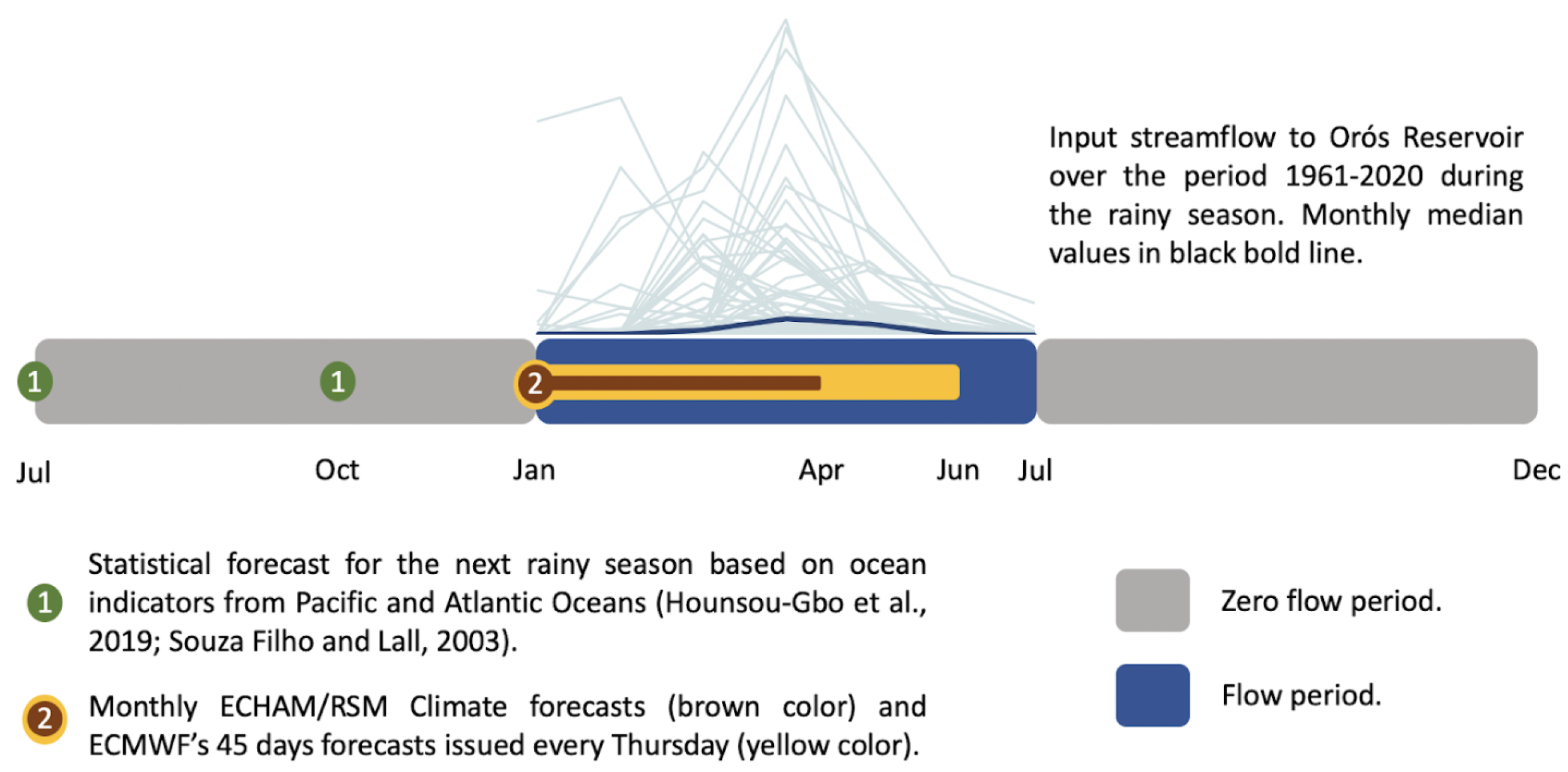
For about 19 years, FUNCEME and COGERH have used a combination of seasonal climate and hydrological models to support reservoir operations. Inflow forecasts are made for key regional river basins in Brazil for water resources planning and in response to drought risk. Current work to improve the seasonal forecast system includes the use of an interannual statistical model and dynamic global and regional models, as well as a recent initiative to use a subseasonal timescale (S2S) (Figure 2). The negotiation process for water allocation commences in early July, the beginning of the dry season in Ceará, and uses statistical rainfall and water flow forecasts issued in July (Water 15 02460 i001) as a basis. These forecasts are updated in October (Water 15 02460 i001). In January (Water 15 02460 i002), another update occurs using dynamic models. From then on, climate and hydrological forecasts are issued monthly until April (Water 15 02460 i002). The time horizon for water allocation discussed in July is 18 months. It focuses on the quality of the rainy season of the following year, as water inflow to the state’s reservoirs is typically not observed from July to December. The forecast system with the S2S approach is not explored in this article. The analysis here focuses on seasonal forecasts issued in January.

3.2. Hydrological Forecasts

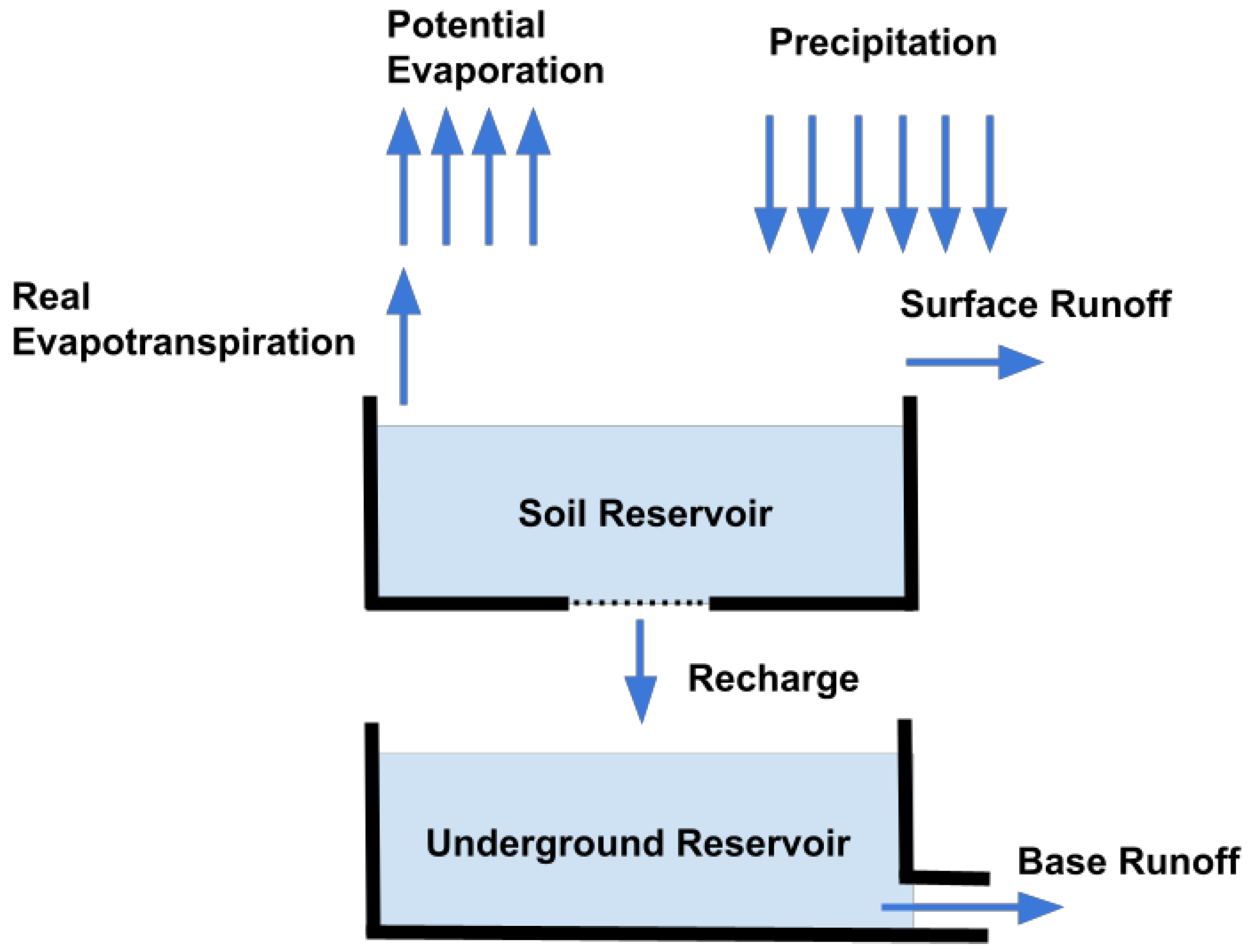
In this work, we use the Soil Moisture Accounting Procedure (SMAP) rainfall-runoff model [40]. The SMAP is a deterministic, lumped hydrologic model with a simple structure that uses two reservoirs to describe water storage and flows through moisture balance at a monthly scale (Figure 3). More information about the model can be found in Barros et al. (2010) [41].
The monthly rainfall-runoff SMAP hydrologic model was calibrated using rainfall, potential evapotranspiration, and available inflow series for the three reservoirs of this study for the period 1986–2010: 1986–2010 for the Orós and Banabuiú Reservoirs and 2002–2010 for the Castanhão Reservoir. These periods were selected based on the availability of monthly streamflow data for each reservoir (as a function of changes in volume, releases, and evapotranspiration of the water body). The monthly inflow data were provided by COGERH. After the calibration, the flows were calculated for the period 1981–2022 using the observed rainfall and potential evaporation series.
The monthly rainfall series were obtained for each basin using the Thiessen polygon method applied to a network of conventional rain gauges monitored by FUNCEME. The potential evapotranspiration series were estimated with the Hargreaves–Samani Equation [42], using monthly temperature data 2 m from the Brazilian National Institute of Meteorology (INMET) network of automatic meteorological stations. The method only requires minimum, average, and maximum temperatures. The Food and Agriculture Organization of the United Nations (FAO) considers this method a way to simplify evapotranspiration calculations in the absence of observed meteorological data required by the Penman–Montheith method [43].
Similarly, SMAP was employed to generate streamflow forecast series for the hindcast period (1981–2010) and the verification period (2011–2022). As input data, the hydrological model used the monthly precipitation and potential evapotranspiration forecasts from January to May (JFMAM) from the ECHAM4.6 model for a set of 20 members. The latter variable was estimated using the same method employed to generate the flows for the observed period [42], although the predicted monthly temperatures derived from the set of members of the ECHAM4.6 were used in this case.
Monthly flows were generated for the incremental basins of the Castanhão, Orós, and Banabuiú Reservoirs and converted to inflows (in cubic hectometers, hm3) into these reservoirs.

3.3. Metrics of Performance

3.3.1. Climate Model

The performance of a climate forecast system cannot be evaluated by comparing an individual probabilistic forecast to its corresponding observed value but rather by assessing the observed variability of signal and noise over a period of time. “Good quality” forecasts can be obtained by properly generating a large ensemble in order to reduce noise. It may also be possible to obtain a good quality forecast by adjusting the forecast using post-processing techniques such as the one used in this article. The evaluation of said forecasts should be based on verification periods or cross-validation experiments and not over the historical period, called hindcasts (i.e., predictions made over a past period using only observations available at that time and that can be used as a basis for the aforementioned post-processing techniques). The performance of the climate model’s rainfall forecasts is evaluated using the Pearson correlation coefficient (CORR) and the Ranked Probability Skill Score (RPSS).
Pearson correlation coefficient (CORR)—To determine the correlation of the forecast and observation during the verification period, the Pearson correlation coefficient (CORR) was used (Equation (1)):
C O R R = i = 1 n ( f c s t f c s t ¯ ) ( r e f r e f ¯ ) i = 1 n ( f c s t f c s t ¯ ) 2 i = 1 n ( r e f r e f ¯ ) 2
where f c s t is the average of the 20 members of the forecast, r e f is the reference (observation or value of the estimated variable based on the observations), n is the number of years used in the series. The bars above these variables indicate the respective average for the entire verification period.
The correlation coefficient takes a value between 1 and 1, where a value of +1 implies perfect positive correlation between the forecast and verification (e.g., more rain than average during the same months and less rain than average during the same months), a value of 1 implies a perfect negative correlation (e.g., the forecast predicts above-average rainfall and the verification results in less-than-average rainfall), and a value of zero indicates no correlation.
Given the proximity of its spatial resolution with the ECHAM4.6 grid, the Climate Prediction Center Merged Analysis of Precipitation (CMAP) monthly precipitation dataset [44] was used to analyze the CORR of the ECHAM4.6 for NEB. The CMAP precipitation database is constructed from remote sensing and station observational data and has a grid spacing of 2.5° × 2.5° for the landmass of the entire globe. For the analysis of the CORR at the level of the reservoirs’ incremental basins, the monthly precipitation from FUNCEME’s network of conventional rain gauges was used.
The Ranked Probability Score (RPS)—Ranked Probability Score (RPS) quantifies the extent to which predicted probabilities deviate from observed outcomes and can demonstrate systematic bias in location and confidence [45,46]. Thus, the score reflects the degree of discrimination, reliability, and resolution. Discrimination between results would be considered successful if higher probabilities were assigned to above-normal precipitation events compared to below-normal precipitation events. On the other hand, systematic locational biases would manifest themselves if the probabilities assigned to above-normal rainfall were very low, while those assigned to below-normal rainfall were very high, even in cases of successful discrimination.
Systematic confidence-level biases would be reflected in forecasts with probabilities that deviate from 0.333, and that exhibit greater confidence than warranted by the degree of discrimination [46]. The use of the value 0.333 in the computation of the Ranked Probability Score (RPS) is related to the concept of a reference forecast. In RPS calculation, the reference forecast is typically a climatological forecast or a simple reference model. Here, the value of 0.333 is derived from a climatological forecast that assumes an evenly distributed probability across all three forecast categories. Further details on RPS are provided below.
The Ranked Probability Score (RPS) is a measure of the precision of a probabilistic forecast. The equation for the RPS is given as:
R P S f c s t = 1 n c a t i c a t = 1 n c a t P c u m f c s t i c a t P c u m o b s i c a t 2
where i c a t is the number of categories (1, 2, or 3), which depends on the forecast categories (below, near, or above normal), and n c a t is the total number of categories, which is usually three in a tercile-based system. The cumulative forecast probability until the category i c a t is represented by P c u m f c s t i c a t . The comparable term for the cumulative probability of the observation is represented by P c u m o b s i c a t . The error is the sum of the squared difference between the cumulative forecast probability and the corresponding observation, where 1 is given to the observed category and 0 to the other categories.
Ranked Probability Skill Score (RPSS)—The Ranked Probability Skill Score (RPSS) is a skill score used to evaluate probabilistic predictions [45,46] (Equation (3), below). It compares the cumulative squared error, or RPS, of a real set of forecasts ( R P S f c s t ) with that of a reference forecast (a constant climatological forecast) for which the probability of each category is 0.333 ( R P S c l i m ).
RPS measures a forecast’s squared error, which indicates to what point a forecast is unsuccessful in discriminating between the different observed results and/or has a systematic location and confidence-level bias. A positive RPSS implies that the RPS is smaller for the forecasts than for the climatological forecasts. Thus, the score reflects discrimination, reliability, and resolution.
Comparing the real and constant climatological forecasts, the orientation of RPSS is reversed from that of the RPS. A higher RPSS indicates that the real forecasts are successful in discriminating between different observed outcomes and are free from systematic location and confidence-level biases when compared to constant climatological forecasts.
The RPSS provides a rigorous and objective measure of the capacity of probabilistic forecasts, which is critical for many applications, including decision-making, risk management, and public safety. RPSS is easy to calculate (see Equation (3)), which makes it a valuable tool to verify forecasts and evaluate models within atmospheric sciences.
R P S S = 1 R P S f c s t R P S c l i m

3.3.2. Hydrological Model

In order to evaluate the hydrological forecasts in this study, we include the verification method proposed by Nash and Sutcliffe (1970) [47], in addition to the metrics cited above. The Nash–Sutcliffe Efficiency (NSE) is widely used to assess the performance of hydrological models, verifying the agreement between observed and predicted values, taking into account systematic and random errors. The NSE varies from − to 1, where values closer to 1 indicate a better fit between the predicted and observed values. NSE values of less than 0 indicate that the model is a worse predictor than the observed mean. In general, values above 0.5 indicate good agreement between the predicted and observed values. NSE is defined as:
N S E = 1 i = 1 n ( Q o b s i Q m o d i ) 2 i = 1 n ( Q o b s i Q o b s ¯ ) 2
where Q o b s is the estimated flow based on observed precipitation and temperature, the latter of which is used to estimate potential evapotranspiration and Q m o d is the flow calculated by the SMAP model Table 2. When presenting the results referring to the inflow forecasts obtained from the unidirectional coupling of each of the 20 members of ECHAM4.6 and the SMAP, Q m o d represents the mean series of this set (Qprev) and Q o b s represents the series modeled from the observed data. That is, the evaluations of the inflow forecast system are based on the comparison between the flows derived from the SMAP model using the observed and predicted hydrometeorological series.

3.4. Reservoir Operations

To analyze the value of the system forecast for reservoir operation, we used a water-allocation decision support system, the Decision Support System for Water Allocation Management (DSS SIGA) [41]. For the experiment carried out here used, the initial reservoir volume was set to 10%, 25%, and 50% capacity. The average demand used was 10.4 m3/s for the Orós and Banabuiú Reservoirs and 28.8 m3/s for the Castanhão Reservoir.
To calculate the reference values during climatology (1981–2010), simulations with releases equal to pre-defined demands were performed using DSS SIGA. These operation simulations were carried out from January to December for the hindcast period (1981–2010) and verification period (2011–2022) using the streamflows estimated from the observations (The streamflows here are estimated using the SMAP model, properly calibrated, from estimated monthly average rainfall and potential evapotranspiration series for the incremental reservoir basin as described in Section 3.2) and forecasts (20 members) for the two periods. Based on the results corresponding to the estimated streamflows during the climatology period (1981–2010), the terciles corresponding to the volumes at the end of December and to the percentage of demands met (33.3% and 66.7%) were calculated. These reference values will be used to evaluate the value of forecasting in operations simulations to meet pre-defined demands.
Likewise, for the predicted streamflows (20 members), DSS SIGA was used to simulate releases corresponding to each member for the period from 1981 to 2022. Initial volumes of 10%, 25%, and 50% maximum capacity of each reservoir were used to simulate operations of each reservoir to meet their respective demands. During the simulations, temporal windows of 12 months, with January as the first month, were used. The value of forecasts with respect to the reference period (1981–2010) was evaluated using the CORR and RPSS metrics, comparing the simulation results based on observed and predicted inflows in terms of reservoir volume at the end of December.

4. Results

4.1. Atmospheric Model Forecasts: Northeast Region

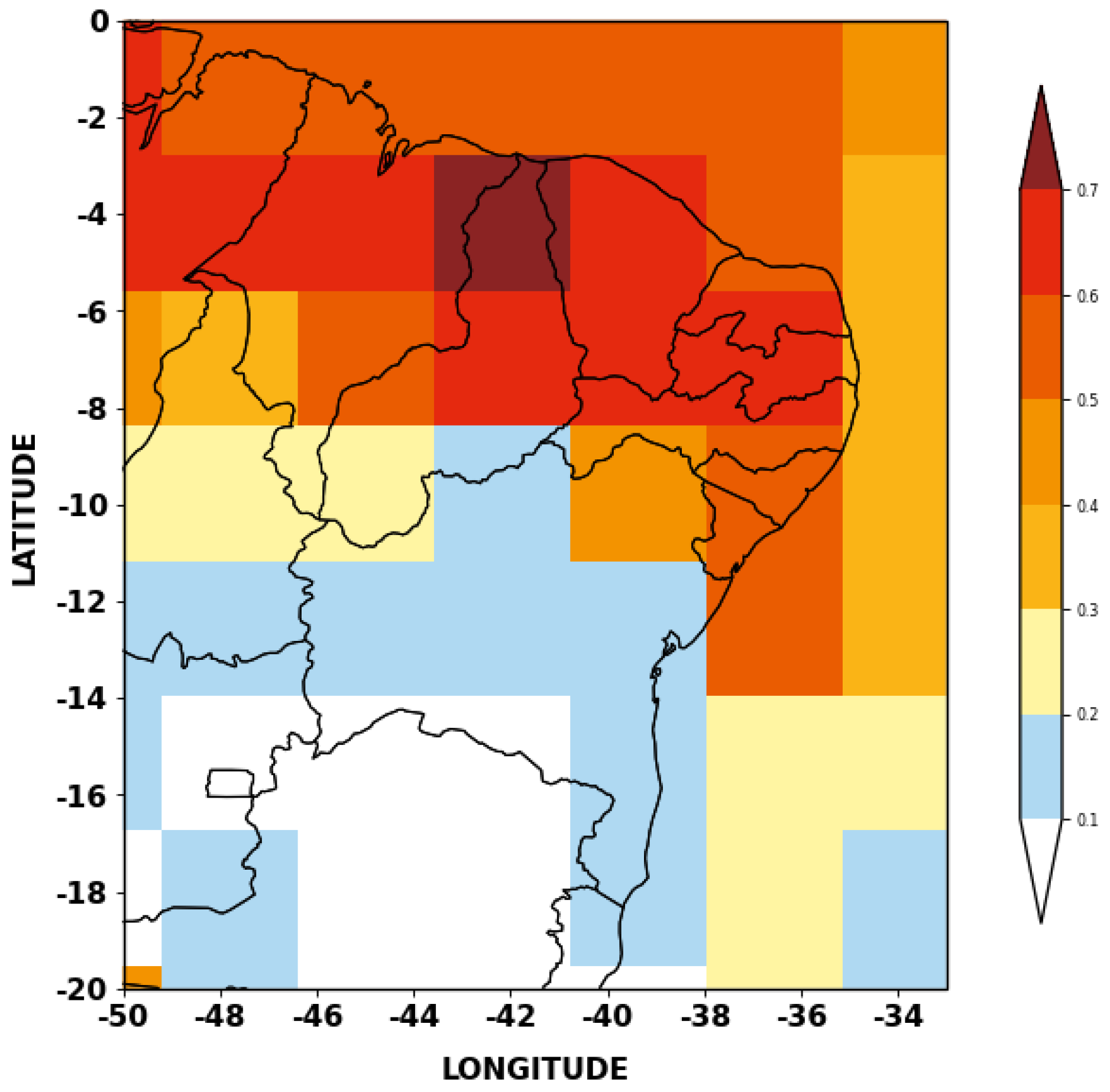
The ensemble mean of the JFMAM precipitation forecasts from the ECHAM4.6 model is in good agreement with the observational dataset for the hindcast period (1981–2010), capturing well the interannual variability for much of the NEB except for the southern part of the region, as shown in the map in Figure 4. The following steps were used to generate the map presented in Figure 4: 1. Preprocessing both datasets (ensemble mean of cumulative rainfall forecasts from ECHAM4.6 model, and CMAP observed rainfall data) in order to align them in terms of spatial resolution, temporal coverage, and format; 2. Calculating the correlation coefficients for each grid cell; and then 3. Mapping the correlation values onto the geographical representation of Northeast Brazil. This process helps visualize the spatial patterns and strength of the relationship between the ensemble mean of cumulative rainfall forecasts and the observed rainfall data.
The spatial distribution of the correlation coefficients shows results above 0.6 for a large part of North NEB in the states of Maranhão (MA), Piauí (PI), Ceará (CE), Rio Grande do Norte (RN), Paraíba (PB), Pernambuco (PE), Sergipe (SE), and Alagoas (AL). This contrasts with the correlation coefficient for the state of Bahia (BA), located in the south of NEB, which had values less than 0.2.

4.2. Atmospheric Model Forecasts: Strategic Reservoir Basins

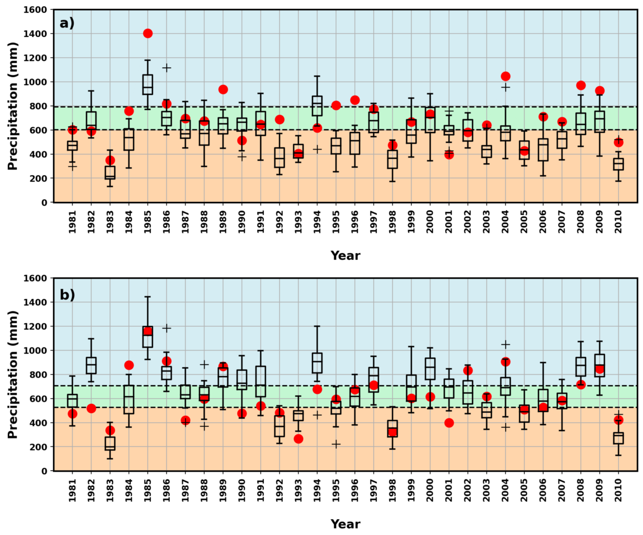
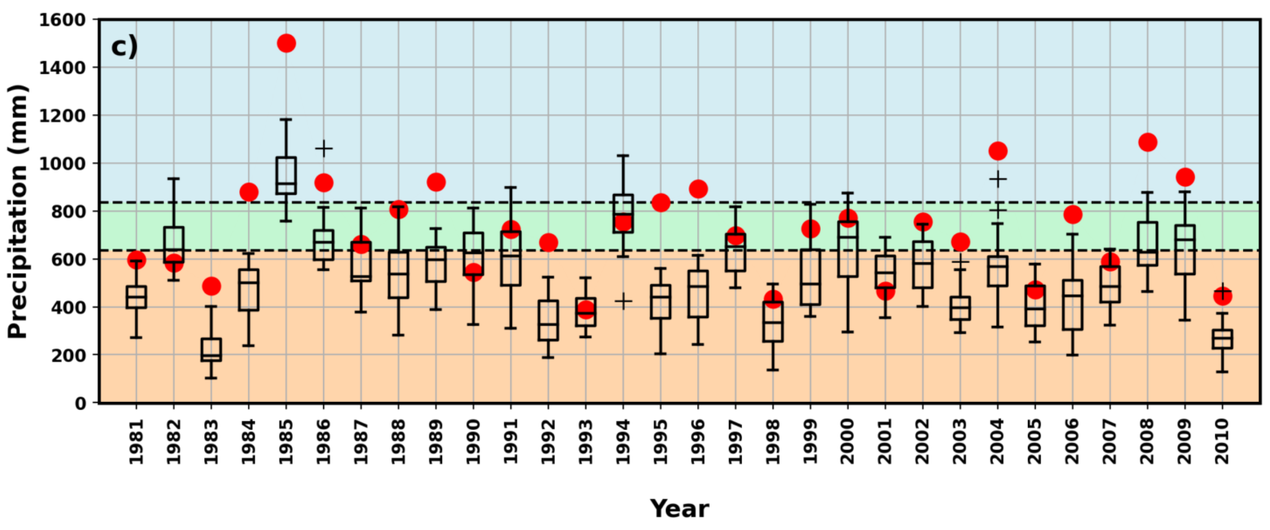
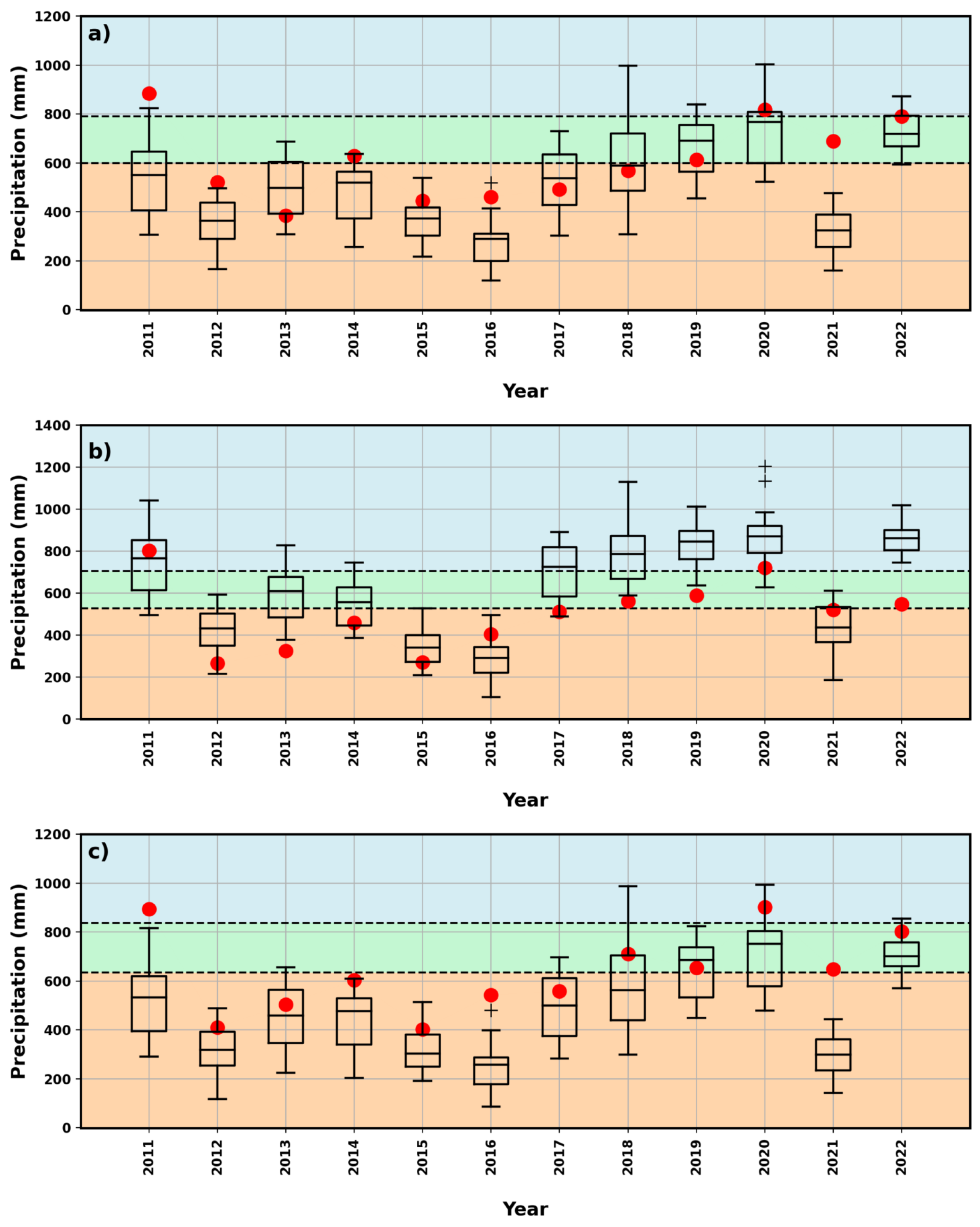
Figure 5 and Figure 6 show the results of the cumulative rainfall forecasts for the period from January to May (JFMAM) for the basins of the three reservoirs (Orós, Banabuiú, and Castanhão) during the hindcast and verification periods, respectively. The dotted horizontal lines represent the 33 and 66 percentiles for the observed climatology (hindcast period of 1981–2010), with the categories below average, around average, and above average corresponding to the colors orange, green, and blue colored shaded areas, respectively. The red dots represent the observed cumulative rainfall values. The plotting of the results of the forecasts per ensemble (20 members) as boxplots is interesting, as it shows the median and interquartile range and still allows for the identification of extreme values. It is also possible to identify the dispersion of the 20 members and, in turn, obtain an idea of the forecast uncertainty of each, even as indicated by the members’ variance. The results indicate that the ECHAM4.6 model was able to capture the interannual variability for the rainfall totals for JFMAM during the hindcast period (1981–2010) and verification period (2011–2022) in the contribution basins of the three reservoirs evaluated in this study. Nonetheless, for the Orós and Castanhão Reservoirs, the atmospheric model had a tendency to underestimate a large portion of the observed events in the period, which is not repeated during the verification period, for which the model achieved less biased results when compared to the observational data (Figure 5a,c and Figure 6a,c). The less biased results during the verification period do not necessarily indicate an improvement in performance. Rather, they could be the result of a verification period (2011–2022) that was actually drier compared to the hindcast period, with half of the years with cumulative rainfall in the below-average category and only two years of rainfall in the above-average category. It is important to note the rough resolution of the model, which covers the state of Ceará with only two grid points. The Castanhão and Orós basins are almost entirely covered by a single grid point in the model, while the Banabuiú basin has significant areas in both grid points.
Table 3 summarizes the results for the forecasts obtained for the JFMAM period using the ECHAM4.6 model for the hindcast, verification, and entire periods, in terms of correlation (CORR) between the ensemble means and the observed values corresponding to these periods. The table includes the results of the RPSS for the same forecasts and observed values for the three periods. The Banabuiú and Castanhão Reservoirs had similar results for CORR in the hindcast and verification periods, while the Orós Reservoir had a smaller correlation, albeit still significant, for the verification period. These results reflect the observed variability captured between the modeled and observed series and can be considered very good, taking into account the model’s resolution. The verification metric adopted to evaluate the probabilistic forecasts of the forecast system (RPSS) shows positive results for the three reservoirs, which indicates that the forecasts add information with respect to the climatology.

4.3. Forecasts of Inflows into the Strategic Reservoirs

For each basin, the estimated inflows based on the observations (Qobs) were obtained using the monthly SMAP model, which was duly calibrated and used observed rainfall and average monthly potential evapotranspiration for the basin as inputs. The model accumulated the flow values obtained during the JFMAM period. The inflow forecasts for each reservoir were obtained using the same calibrated monthly SMAP model. Instead of observation data, seasonal forecasts, represented by the 20 precipitation and potential evapotranspiration members obtained from the ECHAM4.6 model during the hindcast period (1981–2010) and verification period (2011–2022), were used. For the period from June to December, the dry period, the inflows were considered zero in the reservoir operation simulation experiment.
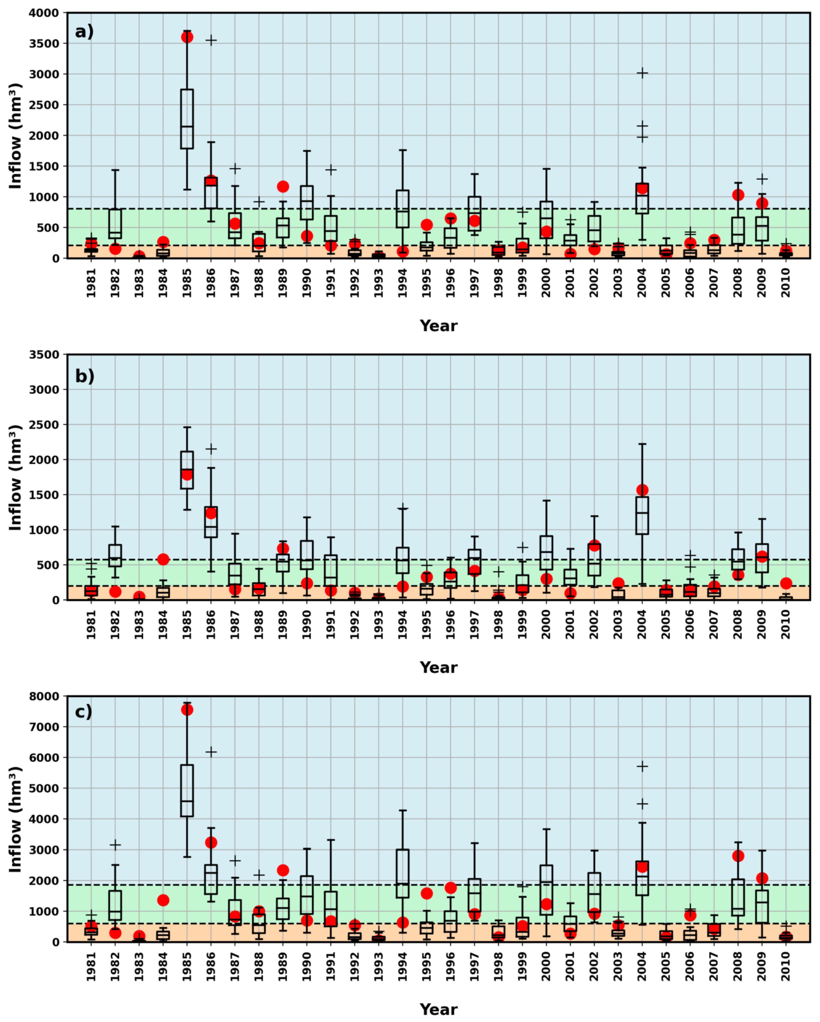
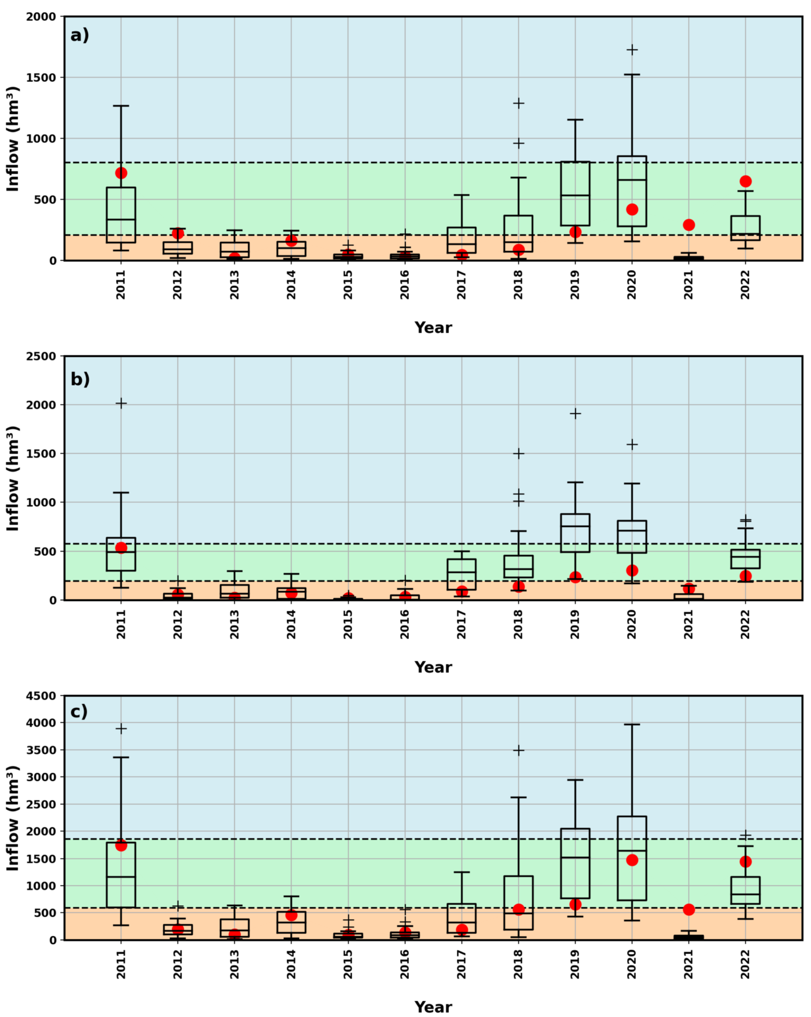
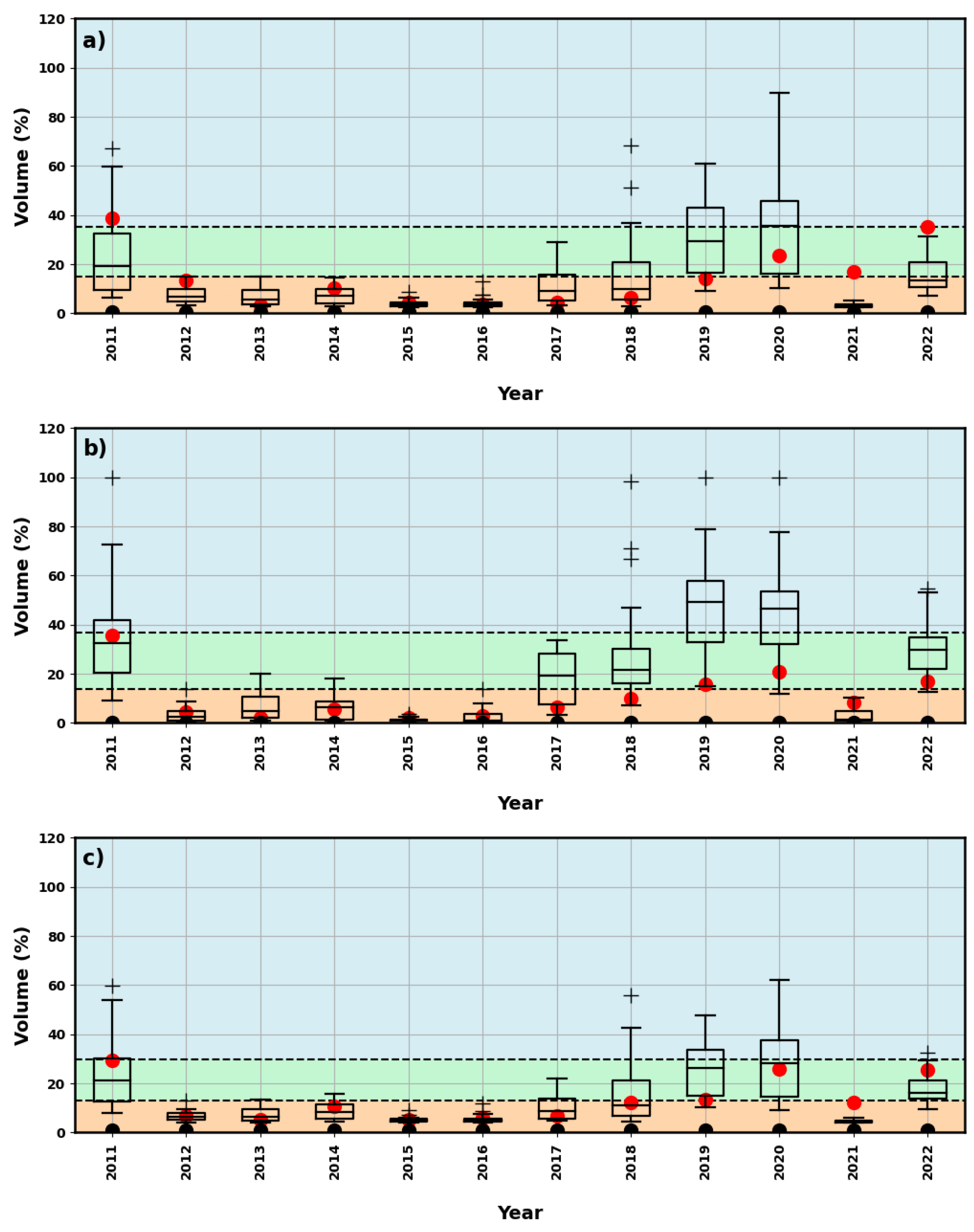
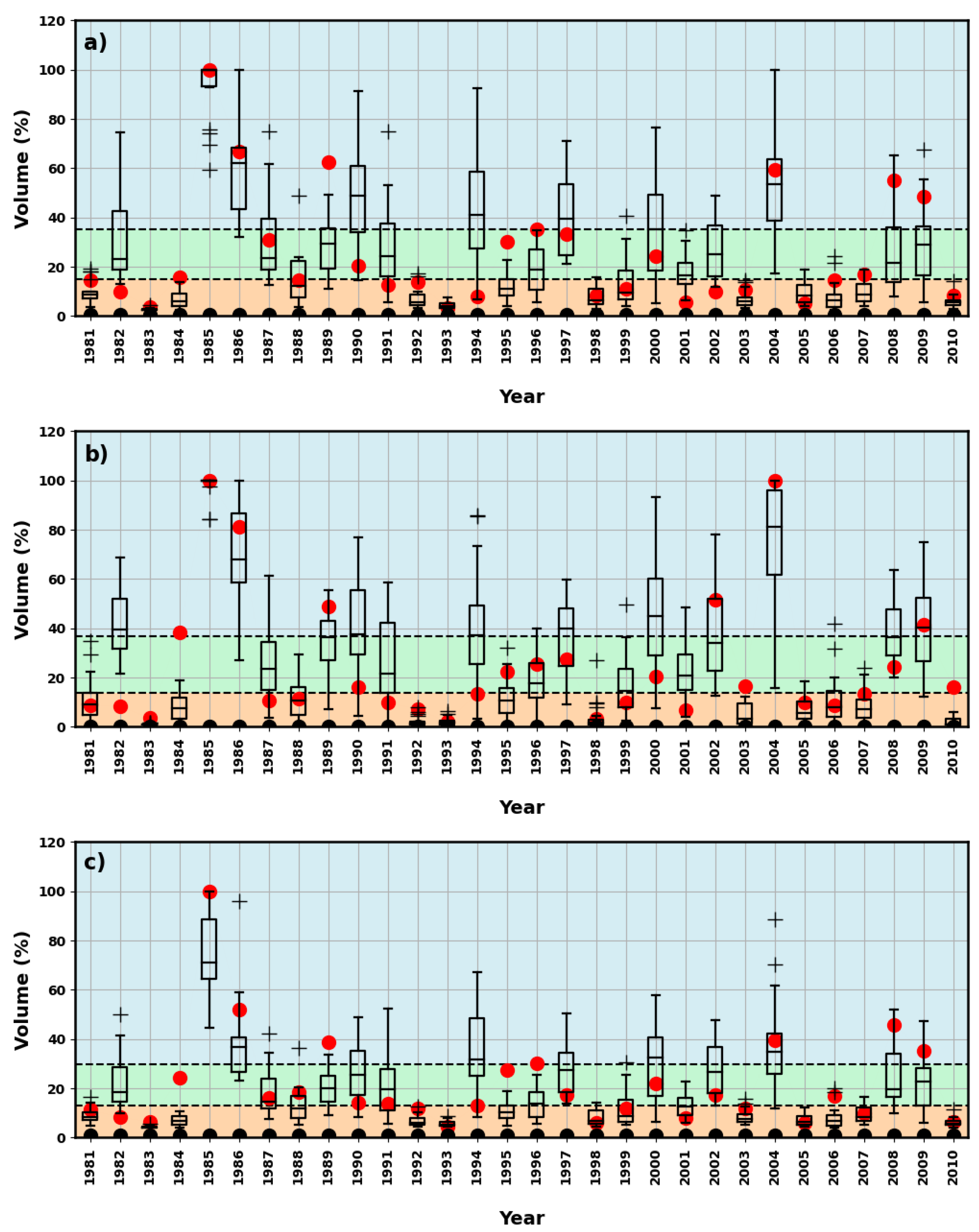
Figure 7 and Figure 8 present the forecasted inflows (Qprev) and estimated inflows (Qobs, red dots) for the JFMAM period for the contribution basin of each of the three reservoirs analyzed. The dotted horizontal lines represent the 33 and 66 percentiles of the Qobs series during the hindcast period, with the categories below average, around average, and above average represented by the colors orange, green, and blue colored shaded areas, respectively. For the hindcast period, despite the low resolution of the climatological model, the interannual variability of the accumulated inflows during the JFMAM period was captured for the contribution basins of the reservoirs. However, there was a tendency to overestimate the inflows into the Orós and Banabuiú Reservoirs and underestimate the inflows into the Castanhão Reservoir. Still keeping the model resolution in perspective, the results for the verification period show that the forecasts capture the interannual variability during the period analyzed (Figure 8), although between 2017 and 2022 (except 2021), the medians of the model members for the Banabuiú Reservoir (Figure 8b) consistently underestimated the observation.
Table 4 summarizes the performance evaluation metrics (NSE, CORR, and RPSS) for the inflow series of the three reservoirs. The inflow forecasts have high correlation coefficients for the hindcast and verification periods, with similar results for the three reservoirs. The RPSS values (around 0.2 for the Orós Reservoir for the verification period and greater than 0.4 for the Orós and Castanhão Reservoirs for the hindcast period) indicate that the models add significant information with respect to the climatology. The hindcast period (1981–2010) and total period (1981–2022) ranged between 0.65 and 0.72. For the verification period (2011–2022), the Banabuiú Reservoir had a negative NSE. This may be attributed primarily to the resolution of the atmospheric model, which resulted in the forecast system indicating a more optimistic scenario (consistently higher inputs than those observed) for the reservoir’s contribution basin. The scenario indicated by the forecasting system cannot be considered optimistic for only three of the twelve years of the short verification period (2011–2022): 2015, 2016, and 2021. In contrast, the NSE values for the Orós and Castanhão Reservoirs were positive, although the value for the Orós Reservoir was low. The RPSS values obtained for the inflow forecasts remained positive for all periods, indicating that the use of probabilistic forecasts for the three reservoirs adds additional information with respect to the climatology.

4.4. Reservoir Operation Incorporating Inflow Forecasts

The importance of the inflow forecasts for water resource management becomes more evident in the context of a multi-year drought, such as the recent drought experienced in the study area (2012–2018). The information in these forecasts is more relevant for the operational planning of key reservoirs when reservoir levels at the beginning of the rainy period are already relatively low. Low reservoir levels at the beginning of the rainy period demand a more careful evaluation during the decision-making process regarding water releases to meet demands. The evaluation should take into consideration the existing risks, based on inflow forecasts, of arriving at the beginning of the following rainy season with a storage volume below a predetermined value. Between the years 1986 and 2022, it was observed that in 19% of the years, the storage level of the Oros Reservoir at the beginning of the year was at or below 15% of its maximum capacity. Similarly, for the Banabuiu Reservoir, this occurred in 38% of the years during the same period. If we only take into consideration the most recent 12-year period (2011–2022), which was selected as the verification period, these values increase to 33% and 75%, respectively, given that it was a very dry period. For the Castanhão Reservoir, these relative frequency values are even higher. The Castanhão Reservoir began the year with a storage level of less than 15% of its capacity in 48% of the years of the total period (2002–2022) and 58% of the years during the verification period (2011–2022).
Figure 9 and Figure 10 present the volume of water stored in the three reservoirs at the end of December, as described in Section 3.4. Reservoir operations simulations were used to obtain these values. An initial volume in January equivalent to 10% of the maximum capacity of each reservoir was assumed for three different streamflow scenarios: forecasted inflow (Qprev) from the forecast system, estimated inflow (Qobs), which are considered the observed inflow here, and zero inflow during the year; a very restrictive situation that may be employed by managers with high aversion to the risk of not meeting demands. The dotted horizontal lines represent the 33 and 66 percentiles of the values identified using the Qobs series during the hindcast period, with the categories below average, around average, and above average represented by the colors orange, green, and blue colored shaded areas, respectively. The red dotted lines represent the estimated volumes for each year. For the three reservoirs, the forecasted volumes at the end of the year follow the interannual variability of the corresponding volumes obtained using the estimated inflows based on the observations during the hindcast period (Figure 9) and verification period (Figure 10). Although the low resolution of the atmospheric model is emphasized here, high RPSS and CORR values were obtained for the forecast when compared to the climatology for the hindcast and verification periods.
The added value of the forecast system, even if based on a low-resolution model, becomes more evident when the zero-inflow scenario is analyzed. The zero-inflow scenario is a conservative water allocation scenario that has been adopted in some states of NEB. Importantly, the use of a conservative zero streamflow scenario could lead to economic losses due to the restrictions imposed on uses. For the zero-streamflow scenario, the Castanhão Reservoir fails partially in August and fully after that month, while the Orós and Banabuiú Reservoirs fail partially in June and fully after that month. With initial volumes of 25% and 50%, the demands associated with the three reservoirs are fully met.
Although not reflected in the results obtained here, for an operation with a horizon of only one year, it seems reasonable to assume that the value of the forecast is very much a function of the initial volume of the reservoir at the beginning of the year and the volume of demand to be met in relation to the capacity of the reservoir. In this context, the simulated operations of the reservoirs with initial volumes of 25% and 50%, whether based on predicted or zero inflow, did not fail to meet the total demand for the three reservoirs. However, the positive RPSS values for the three reservoirs during the hindcast and verification periods presented in Table 5 indicate that the use of inflow forecasts provides additional value to the reference climatology. In turn, the correlation between the flows obtained from the observations and the average of the expected flows for the three reservoirs is around 0.50 for the Orós Reservoir and around 0.70 for the Banabuiú and Castanhão Reservoirs.
The percentages of demands met associated with each reservoir at the end of December were identified using the reservoir operation simulations based on the estimated streamflow with observed data, as well as from each member of the streamflow forecast (see Table 6). For the simulations based on estimated streamflow over the 42 years of the analysis period, the number of years is obtained for each of the four ranges of percent of previously selected demands (ranges: 0↔25 / 25→50 / 50→75 / 75→100; values: 0, 100). When the streamflow forecast is used, the number of forecast members was identified for each year, resulting in a percentage of demands met within each of the ranges. The percentage was calculated by adding the number of members of each range and dividing the result by 20 (the total number of members). In this case, the resulting values represent the average number of years in each range/value indicated by the forecasting system. The values in Table 6 indicate that the use of the forecast system is able to describe the variability of the percent of demands met identified from the estimated streamflows, particularly for the Banabuiú and Castanhão Reservoirs.

5. Conclusions

This study evaluated the climate and hydrological forecast systems used for water allocation in the state of Ceará, specifically focusing on the performance of hydrological forecasting for the Orós, Banabuiú, and Castanhão Reservoirs. The findings of this research highlight several important aspects of these systems.
Firstly, the ECHAM4.6 atmospheric model demonstrated its ability to capture interannual accumulated rainfall variability during the JFMAM period in north NEB, encompassing the state of Ceará. However, it exhibited lower correlation in the southern region. Despite this limitation, positive spatial correlation results were found for the basins contributing to the three reservoirs under evaluation. However, the model’s coarse resolution, which covers the state of Ceará with only two grid points, was a limitation that must be taken into account.
Regarding cumulative rainfall forecasts (JFMAM) for the three reservoir basins, the ECHAM4.6 model performed well in capturing interannual variability during both the hindcast and verification periods. However, it tended to underestimate cumulative rainfall for a significant number of years in the Orós and Castanhão basins during the hindcast period. Nevertheless, the results were less biased for the verification period, indicating a better representation of observed data. This suggests that the model’s performance improved when the verification period exhibited drier conditions.
Objective evaluation using Ranked Probability Skill Score (RPSS) and correlation coefficients (CORR) indicated positive results for all three reservoirs. These results demonstrate that the forecasts provided valuable information beyond climatology, contributing to improved water allocation decisions.
The coupling of precipitation forecasts with the hydrological model proved to be valuable in predicting inflows into the three reservoirs during the JFMAM period, thus facilitating water resource planning and management, particularly during interannual drought periods.
The study also addressed the importance of considering initial reservoir volumes in the decision-making process. It was observed that with larger initial volumes (25% and 50% of capacity), the role of forecasting within a one-year horizon became less crucial due to the magnitude of demands that could be met even under zero inflow assumptions. However, for initial volumes as low as 10% of capacity, the utilization of forecasting provided significant benefits, allowing for a better understanding of inflow variability and improved water-allocation decision-making. Additionally, the use of forecasting in critical situations, where reservoir volumes risk reaching insufficient levels before the rainy season, proved particularly advantageous in preventing unnecessary restrictions on water users and enabling effective water resource management.
Overall, this study emphasizes the importance of climate-hydrological forecasting systems in supporting water allocation processes and mitigating the impacts of water scarcity in drought-prone regions. Continued efforts to enhance the precision and resolution of these models will further improve their reliability and usefulness in water resource management.

Author Contributions

Conceptualization, methodology and validation, J.M.R.P., F.d.C.V.J. and E.S.P.R.M.; software, J.M.R.P. and C.d.C.R.; formal analysis, investigation, writing—original draft preparation, J.M.R.P., F.d.C.V.J. and E.S.P.R.M.; resources, data curation, J.M.R.P.; writing—review, editing and supervision, F.d.C.V.J., D.S.R.J. and E.S.P.R.M. All authors have read and agreed to the published version of the manuscript.

Funding

This study was conducted as part of a collaboration between the PhD program at UFC (Federal University of Ceará) and FUNCEME (Research Institute for Meteorology and Water Resources, State of Ceará). The research was funded by FUNCEME, FUNCAP (Ceará State Science Foundation/Technological Innovation Fund) and the Brazilian Federal Agency for Support and Evaluation of Graduate Education (CAPES).

Data Availability Statement

The study did not report any data.

Conflicts of Interest

The authors declare no conflict of interest.

References

  1. Doblas-Reyes, F.J.; García-Serrano, J.; Lienert, F.; Biescas, A.P.; Rodrigues, L.R.L. Seasonal climate predictability and forecasting: Status and prospects. WIREs Clim. Chang. 2013, 4, 245–268. [Google Scholar] [CrossRef]
  2. Li, H.; Luo, L.; Wood, E.F. Seasonal hydrologic predictions of low-flow conditions over eastern USA during the 2007 drought. Atmos. Sci. Lett. 2008, 9, 61–66. [Google Scholar] [CrossRef]
  3. Sankarasubramanian, A.; Lall, U.; Souza Filho, F.A.; Sharma, A. Improved water allocation utilizing probabilistic climate forecasts: Short-term water contracts in a risk management framework. Water Resour. Res. 2009, 45. [Google Scholar] [CrossRef] [Green Version]
  4. Sharma, K.; Gosain, A. Application of Climate Information and Predictions in Water Sector: Capabilities. Procedia Environ. Sci. 2010, 1, 120–129. [Google Scholar] [CrossRef] [Green Version]
  5. Kaune, A.; Chowdhury, F.; Werner, M.; Bennett, J. The benefit of using an ensemble of seasonal streamflow forecasts in water allocation decisions. Hydrol. Earth Syst. Sci. 2020, 24, 3851–3870. [Google Scholar] [CrossRef]
  6. Martins, E.S.P.R.; Reis Júnior, D.S. Drought Impacts and Policy Responses in Brazil: The Case of the Northeast Region; Special Report on Drought 2021/Global Assessment Report on Disaster Risk Reduction; United Nations: New York, NY, USA, 2021; p. 30. [Google Scholar]
  7. Ceglar, A.; Toreti, A. Seasonal climate forecast can inform the European agricultural sector well in advance of harvesting. NPJ Clim. Atmos. Sci. 2021, 4, 42. [Google Scholar] [CrossRef]
  8. Hamlet, A.F.; Huppert, D.; Lettenmaier, D.P. Economic Value of Long-Lead Streamflow Forecasts for Columbia River Hydropower. J. Water Resour. Plan. Manag. 2002, 128, 91–101. [Google Scholar] [CrossRef]
  9. Kim, K.H.; Shin, Y.; Lee, S.; Jeong, D. Use of Seasonal Climate Forecasts in Agricultural Decision-Making for Crop Disease Management. In Adaptation to Climate Change in Agriculture; Springer: Singapore, 2019; pp. 173–191. [Google Scholar] [CrossRef]
  10. Thomson, M.C.; Doblas-Reyes, F.J.; Mason, S.J.; Hagedorn, R.; Connor, S.J.; Phindela, T.; Morse, A.P.; Palmer, T.N. Malaria early warnings based on seasonal climate forecasts from multi-model ensembles. Nature 2006, 439, 576–579. [Google Scholar] [CrossRef] [Green Version]
  11. Ceccato, P.; Ghebremeskel, T.; Jaiteh, M.; Graves, P.M.; Levy, M.; Ghebreselassie, S.; Ogbamariam, A.; Barnston, A.G.; Bell, M.; del Corral, J.; et al. Malaria stratification, climate, and epidemic early warning in Eritrea. Am. J. Trop. Med. Hyg. 2007, 77, 61–68. [Google Scholar] [CrossRef]
  12. Degallier, N.; Favier, C.; Menkes, C.; Lengaigne, M.; Ramalho, W.M.; Souza, R.; Servain, J.; Boulanger, J.P. Toward an early warning system for dengue prevention: Modeling climate impact on dengue transmission. Clim. Chang. 2010, 98, 581–592. [Google Scholar] [CrossRef]
  13. Lowe, R.; Bailey, T.C.; Stephenson, D.B.; Graham, R.J.; Coelho, C.A.S.; Sá Carvalho, M.; Barcellos, C. Spatio-temporal modelling of climate-sensitive disease risk: Towards an early warning system for dengue in Brazil. Comput. Geosci. 2011, 37, 371–381. [Google Scholar] [CrossRef] [Green Version]
  14. Souza Filho, F.A.; Lall, U. Seasonal to interannual ensemble streamflow forecasts for Ceara, Brazil: Applications of a multivariate, semiparametric algorithm. Water Resour. Res. 2003, 39, 1–13. [Google Scholar] [CrossRef]
  15. Reis, D.; Martins, E.; Nascimento, L.S.; Costa, A.; Alexandre, A. Monthly Streamflow Forecasts for the State of Ceará, Brazil; IAHS-AISH Publication: Wallingford, UK, 2007; pp. 158–166. [Google Scholar]
  16. Block, P.J.; Souza Filho, F.A.; Sun, L.; Kwon, H.H. A streamflow forecasting framework using multiple climate and hydrological models. J. Am. Water Resour. Assoc. 2009, 45, 828–843. [Google Scholar] [CrossRef]
  17. Kwon, H.H.; de Assis de Souza Filho, F.; Block, P.; Sun, L.; Lall, U.; Reis, D.S. Uncertainty assessment of hydrologic and climate forecast models in Northeastern Brazil. Hydrol. Process. 2012, 26, 3875–3885. [Google Scholar] [CrossRef]
  18. de Araújo, C.B.C.; Neto, S.A.D.; Filho, F.D.A.S. Streamflow forecasting for the dam Orós/Ce from hydrometeorological data using perceptrons. Rev. Bras. De Meteorol. 2015, 30, 37–46. [Google Scholar] [CrossRef] [Green Version]
  19. Silveira, C.d.S.; Alexandre, A.M.B.; de Souza Filho, F.d.A.; Vasconcelos Junior, F.d.C.; Cabral, S.L. Monthly streamflow forecast for National Interconnected System (NIS) using Periodic Auto-regressive Endogenous Models (PAR) and Exogenous (PARX) with climate information. RBRH 2017, 22. [Google Scholar] [CrossRef] [Green Version]
  20. Delgado, J.M.; Voss, S.; Bürger, G.; Vormoor, K.; Murawski, A.; Rodrigues Pereira, J.M.; Martins, E.; Vasconcelos Júnior, F.; Francke, T. Seasonal drought prediction for semiarid northeastern Brazil: Verification of six hydro-meteorological forecast products. Hydrol. Earth Syst. Sci. 2018, 22, 5041–5056. [Google Scholar] [CrossRef]
  21. Costa, A.C.; Estacio, A.B.S.; de Souza Filho, F.d.A.; Lima Neto, I.E. Monthly and seasonal streamflow forecasting of large dryland catchments in Brazil. J. Arid Land 2021, 13, 205–223. [Google Scholar] [CrossRef]
  22. Escada, P.; Coelho, C.A.; Taddei, R.; Dessai, S.; Cavalcanti, I.F.; Donato, R.; Kayano, M.T.; Martins, E.S.; Miguel, J.C.; Monteiro, M.; et al. Climate services in Brazil: Past, present, and future perspectives. Clim. Serv. 2021, 24, 100276. [Google Scholar] [CrossRef]
  23. Campos, J.N.B. Secas e políticas públicas no semiárido: Ideias, pensadores e períodos. Estud. Avançados 2014, 28, 65–88. [Google Scholar] [CrossRef] [Green Version]
  24. Erwin De, N.; Engle, N.L.; Magalhães, A.R. Secas no Brasil: Política e Gestão Proativas; Centro de Gestão e Estudos Estratégicos- CGEE - Banco Mundial: Brasília-DF, Brazil, 2016; pp. 37–48. [Google Scholar]
  25. Lemos, M.C.; Puga, B.P.; Formiga-Johnsson, R.M.; Seigerman, C.K. Building on adaptive capacity to extreme events in Brazil: Water reform, participation, and climate information across four river basins. Reg. Environ. Chang. 2020, 20, 53. [Google Scholar] [CrossRef]
  26. Martins, E.S.P.R.; Magalhães, A.R.; Fontenele, D. A seca plurianual de 2010–2017 no Nordeste e seus impactos. Parcerias Estratégicas 2017, 20, 17–40. [Google Scholar]
  27. Martins, E.S.P.R.; Vasconcelos Júnior, F.d.C. O clima da Região Nordeste entre 2009 e 2017: Monitoramento e previsão. Parcerias Estratégicas 2017, 22, 63–80. [Google Scholar]
  28. Hastenrath, S.; Heller, L. Dynamics of climatic hazards in northeast Brazil. Q. J. R. Meteorol. Soc. 1977, 103, 77–92. [Google Scholar] [CrossRef]
  29. Moura, A.D.; Shukla, J. On the Dynamics of Droughts in Northeast Brazil: Observations, Theory and Numerical Experiments with a General Circulation Model. J. Atmos. Sci. 1981, 38, 2653–2675. [Google Scholar] [CrossRef]
  30. Nobre, P.; Srukla, J. Variations of Sea Surface Temperature, Wind Stress, and Rainfall over the Tropical Atlantic and South America. J. Clim. 1996, 9, 2464–2479. [Google Scholar] [CrossRef]
  31. Kane, R.P. Prediction of Droughts in North-East Brazil: Role of ENSO and Use of Periodicities. Int. J. Climatol. 1997, 17, 655–665. [Google Scholar] [CrossRef]
  32. Marengo, J.A.; Torres, R.R.; Alves, L.M. Drought in Northeast Brazil—Past, present, and future. Theor. Appl. Climatol. 2017, 129, 1189–1200. [Google Scholar] [CrossRef]
  33. Roeckner, E.; Arpe, K.; Bengtsson, L.; Christoph, M.; Claussen, M.; Dümenil, L.; Esch, M.; Giorgetta, M.; Schlese, U.; Schulzweida, U. The Atmospheric General Circulation Model ECHAM-4: Model Description and Simulation of Present-Day Climate; Technical report; Max-Planck Institute for Meteorology: Hamburg, Germany, 1996. [Google Scholar]
  34. Gates, W.L. AMIP: The Atmospheric Model Intercomparison Project. Bull. Am. Meteorol. Soc. 1992, 73, 1962–1970. [Google Scholar] [CrossRef]
  35. Gates, W.L.; Boyle, J.S.; Covey, C.; Dease, C.G.; Doutriaux, C.M.; Drach, R.S.; Fiorino, M.; Gleckler, P.J.; Hnilo, J.J.; Marlais, S.M.; et al. An Overview of the Results of the Atmospheric Model Intercomparison Project (AMIP I). Bull. Am. Meteorol. Soc. 1999, 80, 29–56. [Google Scholar] [CrossRef]
  36. Reynolds, R.W.; Rayner, N.A.; Smith, T.M.; Stokes, D.C.; Wang, W. An Improved In Situ and Satellite SST Analysis for Climate. J. Clim. 2002, 15, 1609–1625. [Google Scholar] [CrossRef]
  37. Sun, L.; Moncunill, D.F.; Li, H.; Moura, A.D.; de Assis de Souza Filho, F. Climate downscaling over Nordeste, Brazil, using the NCEP RSM97. J. Clim. 2005, 18, 551–567. [Google Scholar] [CrossRef]
  38. Sun, L.; Li, H.; Zebiak, S.E.; Moncunill, D.F.; Filho, F.D.A.D.S.; Moura, A.D. An Operational Dynamical Downscaling Prediction System for Nordeste Brazil and the 2002–04 Real-Time Forecast Evaluation. J. Clim. 2006, 19, 1990–2007. [Google Scholar] [CrossRef]
  39. White, C.J.; Domeisen, D.I.; Acharya, N.; Adefisan, E.A.; Anderson, M.L.; Aura, S.; Balogun, A.A.; Bertram, D.; Bluhm, S.; Brayshaw, D.J.; et al. Advances in the Application and Utility of Subseasonal-to-Seasonal Predictions. Bull. Am. Meteorol. Soc. 2022, 103, E1448–E1472. [Google Scholar] [CrossRef]
  40. Lopes, J.E.G.; Braga, B.P.F.; Conejo, J.G.L. SMAP—A simplified hydrological model. In Applied Modelling in Catchment Hydrology, Proceedings of the International Symposium on Rainfall-Runoff Modelling; Singh, V.P., Ed.; Water Resources Publications: Littleton, CO, USA, 1982; pp. 167–176. [Google Scholar]
  41. Barros, F.V.F.; Martins, E.S.P.R.; Nascimento, L.S.V.; Reis, D.S. Use of Multiobjective Evolutionary Algorithms in Water Resources Engineering. In Multi-Objective Swarm Intelligent Systems: Theory & Experiences; Springer: Berlin/Heidelberg, Germany, 2010; pp. 45–82. [Google Scholar] [CrossRef]
  42. Hargreaves, G.H.; Samani, Z.A. Reference Crop Evapotranspiration from Temperature. Appl. Eng. Agric. 1985, 1, 96–99. [Google Scholar] [CrossRef]
  43. Allen, R.G.; Pereira, L.S.; Raes, D.; Smith, M. Crop Evapotranspiration: Guidelines for Computing Crop Water Requirements; FAO Irrigation and Drainage Paper; FAO: Rome, Italy, 1998. [Google Scholar]
  44. Xie, P.; Arkin, P.A. Global Precipitation: A 17-Year Monthly Analysis Based on Gauge Observations, Satellite Estimates, and Numerical Model Outputs. Bull. Am. Meteorol. Soc. 1997, 78, 2539–2558. [Google Scholar] [CrossRef]
  45. Epstein, E.S. A Scoring System for Probability Forecasts of Ranked Categories. J. Appl. Meteorol. 1969, 8, 985–987. [Google Scholar] [CrossRef]
  46. Wilks, D.S. Statistical Methods in the Atmospheric Sciences; International Geophysics; Elsevier Science: Amsterdam, The Netherlands, 2011. [Google Scholar]
  47. Nash, J.; Sutcliffe, J. River flow forecasting through conceptual models part I—A discussion of principles. J. Hydrol. 1970, 10, 282–290. [Google Scholar] [CrossRef]
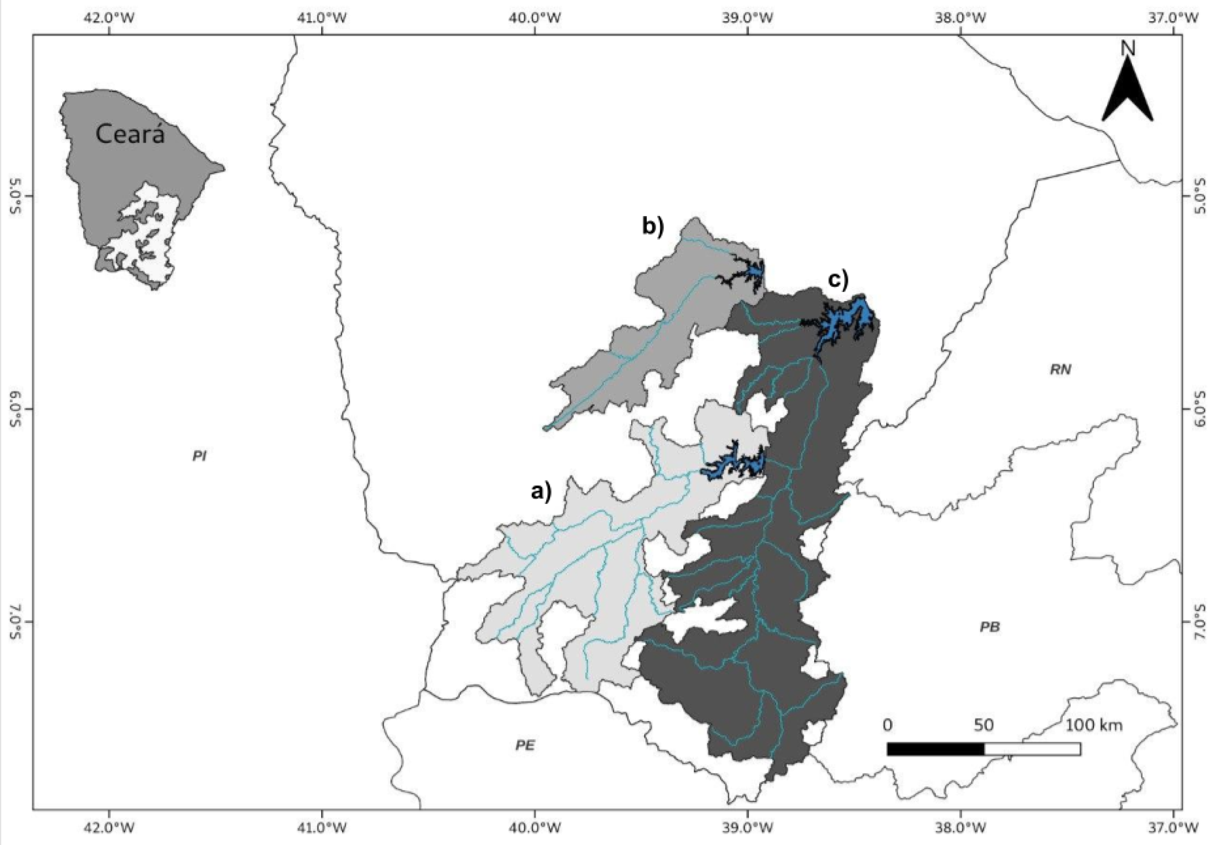
Figure 1. Incremental basin areas of the Orós (a), Banabuiú (b) and Castanhão (c) reservoirs. Source COGERH.
Water 15 02460 g001
Figure 2. Water management in Ceará State, showing the Ceará State inflow forecast system schematic depicting January–April (rainy period) forecasts. The forecast system schematic includes (1) statistical models using previous July and October equatorial Pacific and Atlantic indices and (2) monthly precipitation forecasts from dynamical global and regional seasonal forecast models updated monthly from January to April. The models and forecasts feed a hydrological model to generate monthly flow forecasts (brown) and ECMWF subseasonal precipitation forecasts produced every Thursday for the following 45 days. The results of this model feed a hydrological model to generate daily flow forecasts during the January–May period (yellow). The blue (gray) bar indicates the wet (dry) period [39]; © American Meteorological Society. Used with permission.
Water 15 02460 g002
Figure 3. Conceptual diagram of monthly SMAP model. Flow direction of streamflow, evaporation, and precipitation are indicated by arrows. Source [40].
Water 15 02460 g003
Figure 4. Pearson correlation coefficients (CORR) for the ensemble mean of cumulative rainfall forecasts for JFMAM from the ECHAM4.6 model and CMAP (observed) for Northeast Brazil between 1981 and 2010.
Water 15 02460 g004
Figure 5. Forecasts from the ECHAM4.6 model (boxplots) for cumulative rainfall for JFMAM during the hindcast period for the (a) Orós Reservoir, (b) Banabuiú Reservoir, and (c) Castanhão Reservoir. The dotted horizontal lines represent the 33 and 66 percentiles of the observed climatology, with the categories below average, around average, and above average represented by the colors orange, green, and blue colored shaded areas, respectively. The red dots represent the observed values of cumulative rainfall.
Water 15 02460 g005aWater 15 02460 g005b
Figure 6. Forecasts from the ECHAM4.6 model (boxplots) for cumulative rainfall for JFMAM during the verification period for the (a) Orós Reservoir, (b) Banabuiú Reservoir, and (c) Castanhão Reservoir. The dotted horizontal lines represent the 33 and 66 percentiles of the observed climatology, with the categories below average, around average, and above average represented by the colors orange, green, and blue colored shaded areas, respectively. The red dots represent the observed values of cumulative rainfall.
Water 15 02460 g006
Figure 7. Streamflow forecasts (boxplots) corresponding to the 20 rainfall members of the ECHAM4.6 model, obtained from the SMAP model during the JFMAM period for the (a) Orós Reservoir, (b) Banabuiú Reservoir, and (c) Castanhão Reservoir for the hindcast period. The horizontal dotted lines represent the 33 and 66 percentiles of the observed climatology, with the categories below average, around average, and above average represented by the colors orange, green, and blue colored shaded areas, respectively. The red dots represent the estimated streamflow values for the JFMAM period.
Water 15 02460 g007
Figure 8. Streamflow forecasts (boxplots) corresponding to the 20 rainfall members of the ECHAM4.6 model, obtained from the SMAP model for the JFMAM period for the (a) Orós Reservoir, (b) Banabuiú Reservoir, and (c) Castanhão Reservoir for the forecast period. The horizontal dotted lines represent the 33 and 66 percentiles of the observed climatology, with the categories below average, around average, and above average represented by the colors orange, green, and blue colored shaded areas, respectively. The red dots represent the estimated streamflow values for the JFMAM period.
Water 15 02460 g008
Figure 9. Volumes of the identified reservoirs at the end of December, beginning with 10% capacity at the beginning of January, from the simulated operation of the reservoirs to meet demands based on streamflow forecasts (boxplots) for the hindcast period: (a) Orós, (b) Banabuiú, and (c) Castanhão. The dotted horizontal lines represent the 33 and 66 percentiles referring to the resulting volumes at the end of December for the same period (JFMAM) during the verification period. The categories below average, around average, and above average are represented by the colors orange, green, and blue colored shaded areas, respectively. The red dots represent the volumes at the end of the month of December based on simulated operations using streamflow observed for the JFMAM period, while the black dots are the simulated operations using the hypothetical zero streamflow into the reservoirs.
Water 15 02460 g009
Figure 10. Volumes of the identified reservoirs at the end of December, beginning with 10% capacity at the beginning of January, from the simulated operation of the reservoirs to meet demands based on streamflow forecasts (boxplots) for the verification period: (a) Orós, (b) Banabuiú, and (c) Castanhão. The dotted horizontal lines represent the 33 and 66 percentiles referring to the resulting volumes at the end of December for the same period (JFMAM) during the verification period. The categories below average, around average, and above average are represented by the colors orange, green, and blue colored shaded areas, respectively. The red dots represent the volumes at the end of the month of December based on simulated operations using streamflow observed for the JFMAM period, while the black dots are the simulated operations using the hypothetical zero streamflow into the reservoirs.
Water 15 02460 g010
Table 1. Basic Data and Statistics for Accumulated Inflow of the Orós, Banabuiú, and Castanhão Reservoirs from January to June. Source COGERH.
Reservoir
OrósBanabuiúCastanhão
Total Basin Area (km2)24,960.9214,244.2244,806.33
Storage (hm3)194016016700
Q10 (hm3)67.518.57153.84
Q25 (hm3)129.0827.15199.17
Median (hm3)322.0190.27323.69
Q75 (hm3)758.72535.051139.6
Q90 (hm3)1438.06836.181904.24
Mean (hm3)628.21331.48877.16
Standard Deviation (hm3)831.6495.611189.73
Table 2. Nash–Sutcliffe Efficiency and correlation between observed and SMAP-modeled monthly inflows for the Orós, Banabuiú, and Castanhão Reservoirs.
Reservoir1986–20102011–20221986–2022
NSECORRNSECORRNSECORR
Orós0.810.950.280.960.800.95
Banabuiú0.450.660.500.800.520.70
Castanhão0.700.870.830.910.870.81
Note: All available data from the period 1986 to 2022 were used in the calculation of the metrics. For the Castanhão Reservoir, the beginning of the observed series was in 2002.
Table 3. Evaluation of the performance metrics for the rainfall forecasts during the JFMAM period, using the ECHAM4.6 model for the contribution basins of the Orós, Banabuiú, and Castanhão Reservoirs.
Reservoir1981–20102011–20221981–2022
RPSSCORRRPSSCORRRPSSCORR
Orós0.130.610.310.500.190.60
Banabuiú0.260.660.380.670.300.66
Castanhão0.160.640.320.660.210.66
Table 4. The performance evaluation metrics for the streamflow forecasts for the Orós, Banabuiú, and Castanhão Reservoirs for the JFMAM period, obtained through the unidirectional coupling of the ECHAM4.6 model and the monthly SMAP hydrological model.
Reservoir1981–20102011–20221981–2022
NSERPSSCORRNSERPSSCORRNSERPSSCORR
Orós0.690.190.820.120.430.470.680.250.81
Banabuiú0.720.240.83−1.400.180.710.660.220.81
Castanhão0.650.440.800.590.490.730.660.460.81
Table 5. Performance evaluation metrics for the volumes at the end of May of the Orós, Banabuiú, and Castanhão Reservoirs, identified using the simulated operations of the reservoirs for forecasted and observed inflows into the reservoirs.
ReservoirInitial Volume1981–20102011–20221981–2022
RPSSCORRRPSSCORRRPSSCORR
Orós10%0.240.730.260.470.250.73
25%0.240.690.260.470.240.70
50%0.270.640.260.480.270.65
Banabuiú10%0.250.790.460.690.310.78
25%0.250.760.460.690.310.75
50%0.230.690.430.690.290.69
Castanhão10%0.300.770.560.700.370.78
25%0.290.740.530.730.360.76
50%0.250.670.410.720.290.70
Table 6. Average number of years in each range/percent of the demands met at the end of the December for the Orós, Banabuiú, and Castanhão Reservoirs, identified using the simulated operations for the forecasted and observed inflows into the reservoirs.
ReservoirInfo% Demands Met at the end of December *
=00↔2525→5050→7575→100=100
OrósFcst.18.719.30.60.421.921.5
Obs.1114122525
BanabuiúFcst.18.519.00.50.222.422.1
Obs.1820002221
CastanhãoFcst.15.616.70.40.624.323.8
Obs.912003030
* Arrow indicates that the limit is included in the interval.
Disclaimer/Publisher’s Note: The statements, opinions and data contained in all publications are solely those of the individual author(s) and contributor(s) and not of MDPI and/or the editor(s). MDPI and/or the editor(s) disclaim responsibility for any injury to people or property resulting from any ideas, methods, instructions or products referred to in the content.