
Diel Variation of Phytoplankton Communities in the Northern South China Sea under the Effect of Internal Solitary Waves and Its Response to Environmental Factors

Abstract
1. Introduction
2. Materials and Methods
2.1. Field Data Collection
2.2. Phytoplankton Data
2.3. Data Analysis
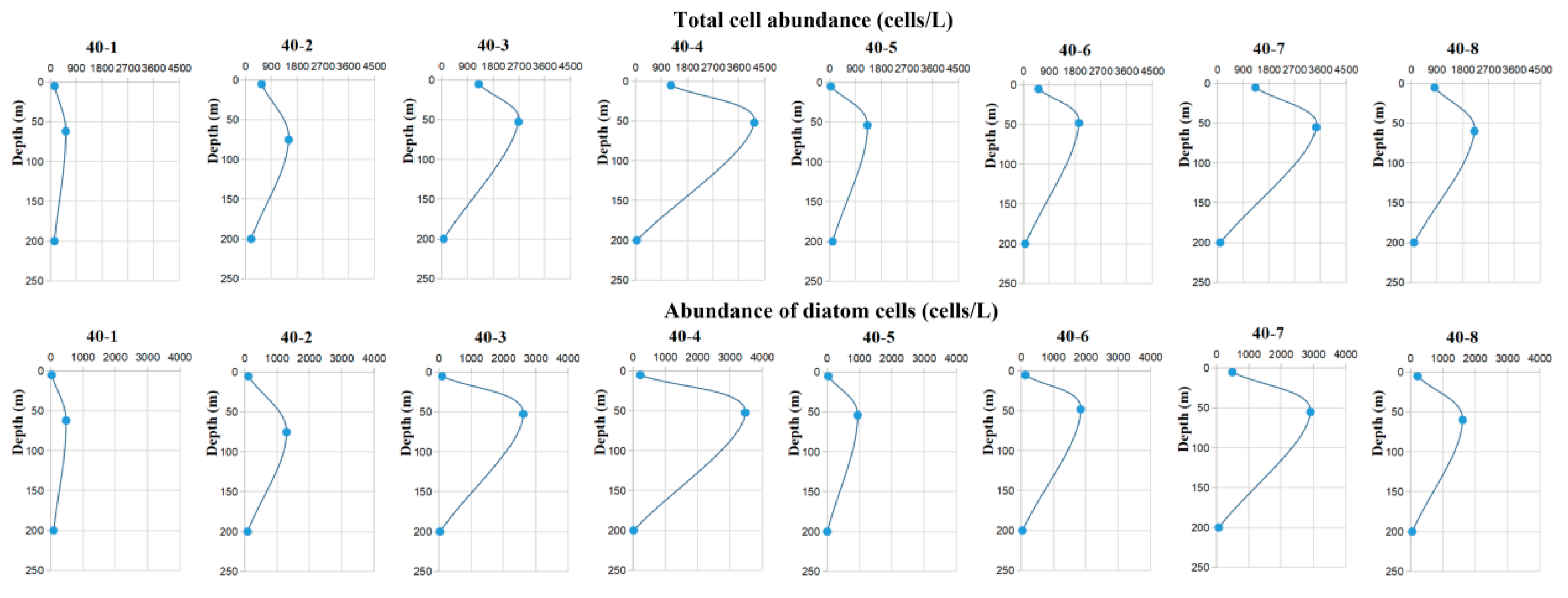
3. Results
3.1. Composition of Phytoplankton Species
3.2. Vertical Distribution of Phytoplankton under the Influence of ISWs
3.2.1. Q40 Station
3.2.2. Q39 Station
3.3. Effect of ISWs on Dominant Species
3.4. Changes in Phytoplankton Species
3.5. Diversity and Evenness Indices
3.5.1. Q40 Station
3.5.2. Q39 Station
3.6. Community Structure Cluster Analysis
3.7. Correlation between Phytoplankton and Environmental Factors
4. Discussion
4.1. Effect of ISWs on Phytoplankton and Dominant Species
4.2. Response of Four Functional Groups to Environmental Factor Changes under the Effect of ISWs
5. Conclusions
Author Contributions
Funding
Data Availability Statement
Acknowledgments
Conflicts of Interest
Appendix A

| Taxa | Volume (μm3) | Nutritional Type | Ecological Group |
|---|---|---|---|
| Group1 | |||
| Cochlodinium spp. | 100,000–1,000,000 | HN | BT |
| Gymnodinium spp. | <10,000 | HN | BT |
| Protoperidinium spp. | 10,000–100,000 | HN | BT |
| Karenia mikimotoi | 10,000–100,000 | HN | BT |
| Karenia brevis | 10,000–100,000 | HN | BT |
| Gyrodinium dominans | 10,000–100,000 | HN | BT |
| Gyrodinium spp. | 10,000–100,000 | HN | BT |
| Group2 | |||
| Chaetoceros debilis | <10,000 | AN | NT |
| Chaetoceros densus | 10,000–100,000 | AN | NT |
| Thalassiothrix longissima | 10,000–100,000 | AN | BT |
| Synedra spp. | 10,000–100,000 | AN | BT |
| Chaetoceros lorenzianus | 10,000–100,000 | AN | BT |
| Chaetoceros spp. | 10,000–100,000 | AN | BT |
| Chaetoceros rostratus | 10,000–100,000 | AN | BT |
| Oxytoxum turbo | 10,000–100,000 | AN | WW |
| Group3 | |||
| Dictyocha speculum | <10,000 | MN | BT |
| Pronoctiluca pelagica | <10,000 | MN | WW |
| Group4 | |||
| Pseudo-nitzschia pungens | <10,000 | AN | WW |
| Oxytoxum mitra | <10,000 | AN | WW |
| Oxytoxum curvatum | <10,000 | AN | WW |
| Chaetoceros femur | <10,000 | AN | WW |
| Chaetoceros atlanticus | <10,000 | AN | WW |
| Chaetoceros atlanticus var. neapolitana | <10,000 | AN | WW |
| Thalassiosira spp. | <10,000 | AN | BT |
| Thalassionema nitzschioides | <10,000 | AN | BT |
| Thalassionema frauenfeldii | <10,000 | AN | BT |
| Skeletonema costatum | <10,000 | AN | BT |
| Scrippsiella trochoidea | <10,000 | AN | BT |
| Prorocentrum minimun | <10,000 | AN | BT |
| Prorocentrum dentatum | <10,000 | AN | BT |
| Oxytoxum crassum | <10,000 | AN | BT |
| Nitzschia longissima | <10,000 | AN | BT |
| Nitzschia spp. | <10,000 | AN | BT |
| Dinophyta | Protoperidinium simulum (Paulsen) Balech, 1974 |
| Alexandrium minutum Halim, 1960 | Protoperidinium spp. |
| Alexandrium spp. | Pyrocystis noctiluca Murray ex Haeckel |
| Alexandrium tamarense (Lebour) Balech, 1985 | Pyrophacus steinii (Schiller) Wall & Dale |
| Amphisolenia schroederi Kofoid | Scrippsiella trochoidea (Stein) Balech ex Loeblich III |
| Blepharocysta splendor-maris (Ehrenberg) Ehrenberg | Bacillariophyta |
| Ceratocorys bipes (Cleve) Kofoid, 1910 | Actinoptychus hexagonus Grunow in Schmidt, 1874 |
| Ceratocorys horrida Stein, 1883 | Actinoptychus senarius (Ehr.) Ehrenberg |
| Cochlodinium brandtii Wulff | Arachnoidiscus ehrenbergii Bailey ex Ehrenberg |
| Cochlodinium polykrikoides Margelef | Asteromphalus flabellatus (Brébisson) Greville, 1859 |
| Cochlodinium spp. | Bacteriastrum comosum Pavillard |
| Corythodinium belgicae (Meunier) F.J.R.Taylor, 1976 | Bacteriastrum furcatum Shadbolt, 1854 |
| Corythodinium carinatum (Gaarder) F.J.R.Taylor, 1976 | Bacteriastrum hyalinum Lauder |
| Corythodinium constrictum (Stein) Taylor | Bacteriastrum mediterraneum Pavillard |
| Corythodinium curvicaudatum (Kofoid) F.J.R.Taylor, 1976 | Biddulphia pellucida Castracane, 1886 |
| Corythodinium latum (Gaarder) F.J.R.Taylor, 1976 | Cerataulina bergonii Ostenfeld, 1903 |
| Corythodinium reticulatum (Stein) Taylor, 1976 | Chaetoceros affinis Lauder |
| Corythodinium spp. | Chaetoceros atlanticus Cleve |
| Corythodinium tesselatum (Stein) Loeblich Jr.& Loeblich III | Chaetoceros atlanticus var. neapolitana (Schröder) Hustedt |
| Dinophysis acuminata Claparède et Lachmann | Chaetoceros buceros Karsten |
| Dinophysis favus (Kofoid & Michener) Balech | Chaetoceros castracanei Karsten |
| Dinophysis oviformis Chen & Ni, 1988 | Chaetoceros coarctatus Lauder |
| Dinophysis parva Schiller | Chaetoceros constrictus Gran |
| Dinophysis spp. | Chaetoceros danicus Cleve |
| Diplopsalopsis bomba (Stein ex Jorgensen) Dodge & Toriumi | Chaetoceros debilis Cleve |
| Dolichodinium lineatum (Kofoid & Michener) Kofoid & Adamson, 1933 | Chaetoceros densus (Cleve) Cleve, 1899 |
| Gonyaulax cochlea Meunier, 1919 | Chaetoceros denticulatus Lauder |
| Gonyaulax kofoidii Pavillard, 1909 | Chaetoceros distans Cleve |
| Gonyaulax macroporus Mangin, 1922 | Chaetoceros femur Schütt |
| Gonyaulax minuta Kofoid & Michener, 1911 | Chaetoceros hirundinellus Qian |
| Gonyaulax monospina Rampi, 1951 | Chaetoceros lauderi Ralfs |
| Gonyaulax ovalis Schiller, 1929 | Chaetoceros lorenzianus Grunow |
| Gonyaulax pacifica Kofoid, 1907 | Chaetoceros messanensis Castracane |
| Gonyaulax polygramma Stein, 1883 | Chaetoceros paradoxus Cleve |
| Gonyaulax spinifera (Claparede & Lachmann) Diesing, 1866 | Chaetoceros pelagicus Cleve |
| Gonyaulax spp. | Chaetoceros peruvianus Brightwell |
| Gonyaulax turbynei Murray & Whitting, 1899 | Chaetoceros pseudodichaeta Ikari |
| Gymnodinium spp. | Chaetoceros rostratus Lauder |
| Gyrodinium dominans Hulbert | Chaetoceros saltans Cleve |
| Gyrodinium falcatum Kofoid & Swezy, 1921 | Chaetoceros spp. |
| Gyrodinium instriatum Freudenthal et Lee | Corethron criophilum Castracane |
| Gyrodinium spirale (Bergh) Kofoid et Swezy | Coscinodiscus asteromphalus Ehrenberg |
| Gyrodinium spp. | Coscinodiscus granii Grough |
| Heterocapsa triquetra (Ehrenberg) Stein, 1883 | Coscinodiscus jonesianus (Greville) Ostenfeld |
| Heterodinium agassizii Kofoid | Coscinodiscus radiatus Ehrenberg |
| Heterodinium milneri (Murray & Whitting) Kofoid, 1906 | Coscinodiscus spp. |
| Heterodinium whittingiae Kofoid, 1906 | Cylindrotheca closterium (Ehrenberg) Reimann & J.C. Lewin, 1964 |
| Histioneis gregoryi Böhm | Diploneis bombus Ehrenberg |
| Karenia brevis (Davis) G.Hansen & Moestrup | Eucampia cornuta (Cleve) Grunow |
| Karenia mikimotoi Hansen & Moestrup | Eunotogramma debile Grunow in Van Heurck, 1883 |
| Lingulodinium polyedrum (Stein) Dodge | Fragilaria spp. |
| Lissodinium spp. | Fragilariopsis doliolus (Wallich) Medlin & Sims |
| Lissodinium taylorii Carbonell-Moore, 1993 | Guinardia flaccida (Castracane) Peragallo |
| Neoceratium boehmii (Graham et Bronikovsky) | Guinardia striata (Stolterfoth) Hasle et al. |
| Neoceratium horridum (Gran) Gómez, Moreira & López-Garcia | Helicotheca tamesis (Shrubsole) Ricard |
| Neoceratium kofoidii (Jörgensen) Gómez, Moreira & López-Garcia | Hemiaulus hauckii Grunow ex Van Heurck, 1882 |
| Neoceratium longipes (Bailey) Gómez, Moreira & López-Garcia | Hemiaulus membranacus Cleve |
| Neoceratium setaceum (Jörgensen) Gómez, Moreira & López-Garcia | Hemiaulus sinensis Greville |
| Neoceratium teres (Kofoid) Gómez, Moreira & López-Garcia | Leptocylindrus danicus Cleve |
| Ornithocercus thumii (Schmidt) Kofoid & Skogsberg | Leptocylindrus mediterraneus (H. Peragallo) Hasle |
| Oxytoxum crassum Schiller | Mastogloia rostrata (Wallich) Hustedt |
| Oxytoxum curvatum (Kofoid) Kofoid, 1911 | Navicula membranacea Cleve, 1897 |
| Oxytoxum depressum Schiller, 1937 | Navicula spp. |
| Oxytoxum elongatum Wood, 1963 | Nitzschia longissima (Brébisson) Ralfs, 1861 |
| Oxytoxum laticeps Schiller | Nitzschia lorenziana Grunow |
| Oxytoxum longiceps Schiller | Nitzschia panduriformis Hustedt in Schmidt et al., 1921 |
| Oxytoxum milneri Murray & Whitting, 1899 | Nitzschia spp. |
| Oxytoxum mitra Stein, 1883 | Odontella sinensis (Greville) Grunow |
| Oxytoxum mucronatum Hope, 1954 | Palmeria hardmaniana Greville |
| Oxytoxum parvum Schiller, 1937 | Paralia sulcata (Ehrenberg) Cleve, 1873 |
| Oxytoxum sceptrum (Stein) Schröder | Pinnularia spp. |
| Oxytoxum scolopax Stein | Planktoniella formosa Qian & Wang |
| Oxytoxum sphaeroideum Stein | Planktoniella sol Qian et Wang |
| Oxytoxum spp. | Pleurosigma acutum Norman |
| Oxytoxum turbo Kofoid | Pleurosigma pelagicum Peragallo |
| Oxytoxum variabilis Schiller | Pleurosigma spp. |
| Palaeophalacroma unicinctum Schiller, 1928 | Pseudo-nitzschia pungens (Grunow ex Cleve) Hasle |
| Podolampas bipes Stein | Rhabodonema adriaticum Kützing |
| Podolampas palmipes Stein | Rhizosolenia alata f. indica (Peragallo) Ostenfeld |
| Pronoctiluca pelagica Fabre-Domerqne | Rhizosolenia bergonii Peragallo |
| Pronoctiluca spinifera (Lohmann) Schiller, 1932 | Rhizosolenia sinensis Qian |
| Prorocentrum compressum (Ostenfeld) Abé | Rhizosolenia styliformis Brightwell |
| Prorocentrum dentatum Stein | Skeletonema costatum (Greville) Cleve |
| Prorocentrum lenticulatum (Matzenauer) Taylor | Synedra spp. |
| Prorocentrum lima (Ehrenberg) Dodge | Thalassionema frauenfeldii (Grunow) Hallegraeff |
| Prorocentrum minimun (Pavillard) Schiller | Thalassionema nitzschioides Grunow |
| Prorocentrum sigmoides Böhm | Thalassiosira eccentrica (Ehrenberg) Cleve, 1904 |
| Prorocentrum spp. | Thalassiosira spp. |
| Prorocentrum triestinum Schiller | Thalassiothrix longissima Cleve et Grunow |
| Protoceratium areolatum Kofoid | Triceratium affine Grunow |
| Protoperidinium conicum (Gran) Balech | Triceratium favus Ehrenberg |
| Protoperidinium excentricum (Paulsen) Balech, 1974 | Dictyochophyceae |
| Protoperidinium orientale (Matzenauer) Balech | Dictyocha fibula Ehrenberg |
| Protoperidinium ovum (Schiller) Balech, 1974 | Dictyocha speculum Ehrenberg |
| Protoperidinium pyrum (Balech) Balech |
References
- McGillicuddy, D.J.; Robinson, A.R. Eddy-induced nutrient supply and new productivity in the Sargasso Sea. Deep Sea Res. (Part I) 1997, 44, 1427–1450. [Google Scholar] [CrossRef]
- McGillicuddy, D.J.; Robinson, A.R.; Siegel, D.A.; Jannasch, H.W.; Johnson, R.; Dickey, T.D.; McNeil, J.; Michaels, A.F.; Knap, A.H. Influence of mesoscale eddies on new productivity in the Sargasso Sea. Nature 1998, 394, 263–265. [Google Scholar] [CrossRef]
- Lin, I.; Liu, W.T.; Wu, C.C.; Wong, G.T.F.; Hu, C.; Chen, Z.; Liang, W.D.; Yang, Y.; Liu, K.K. New evidence for enhanced ocean primary productivity triggered by tropical cyclone. Geophys. Res. Lett. 2003, 30, 1718. [Google Scholar] [CrossRef]
- Cipollini, P.; Cromwell, C.; Challenor, P.G.; Raffaglio, S. Rossby waves detected in global ocean colour data. Geophys. Res. Lett. 2001, 28, 323–326. [Google Scholar] [CrossRef]
- Uz, B.M.; Yoder, J.A.; Osychny, V. Pumping nutrients to ocean surface waters by the action of propagating planetary waves. Nature 2001, 409, 597–600. [Google Scholar] [CrossRef]
- Muench, K.; Lipscomb, M.; Lee, M.; Kuehl, G. Homologous cysteine-containing sequences in tryptophanyl-tRNA synthetases from Escherichia coli and human placentas. Science 1975, 187, 1089–1091. [Google Scholar] [CrossRef]
- Holligan, P.M.; Pingree, R.D.; Mardell, G.T. Oceanic solitons, nutrient pulses and phytoplankton growth. Nature 1985, 314, 348–350. [Google Scholar] [CrossRef]
- Liu, C.T.; Pinkel, R.; Hsu, M.K.; Klymak, J.M.; Chien, H.W.; Villanoy, C. Nonlinear internal waves from the Luzon Strait. Eos Trans. AGU 2006, 87, 449–451. [Google Scholar] [CrossRef]
- da Silva, J.C.B.; New, A.L.; Srokosz, M.A.; Smyth, T.J. On the observability of internal tidal waves in remotely-sensed ocean colour data. Geophys. Res. Lett. 2002, 29, 1569. [Google Scholar] [CrossRef]
- Wang, Y.H.; Dai, C.F.; Chen, Y.Y. Physical and ecological processes of internal waves on an isolated reef ecosystem in the South China Sea. Geophys. Res. Lett. 2007, 34, L18609. [Google Scholar] [CrossRef]
- Wilson, C. Chlorophyll anomalies along the critical latitude at 30°N in the NE Pacific. Geophys. Res. Lett. 2011, 38. [Google Scholar] [CrossRef]
- Pan, X.; Wong, G.T.; Shiah, F.K.; Ho, T.Y. Enhancement of biological productivity by internal waves: Observations in the summertime in the northern South China Sea. J. Oceanogr. 2012, 68, 427–437. [Google Scholar] [CrossRef]
- Chang, M.H.; Lien, R.C.; Tang, T.Y.; D’Asaro, E.A.; Yang, Y.J. Energy flux of nonlinear internal waves in northern South China Sea. Geophys. Res. Lett. 2006, 33. Available online: https://agupubs.onlinelibrary.wiley.com/doi/full/10.1029/2005GL025196 (accessed on 25 May 2023). [CrossRef]
- Chao, S.Y.; Ko, D.S.; Lien, R.C.; Shaw, P.T. Assessing the west ridge of Luzon Strait as an internal wave mediator. J. Oceanogr. 2007, 63, 897–911. [Google Scholar] [CrossRef]
- Hsu, M.K.; Liu, A.K.; Liu, C. A study of internal waves in the China Seas and Yellow Sea using SAR. Cont. Shelf Res. 2000, 20, 389–410. [Google Scholar] [CrossRef]
- Zhang, Z.; Fringer, O.B.; Ramp, S.R. Three dimensional, nonhydrostatic numerical simulation of nonlinear internal wave generation and propagation in the South China Sea. J. Geophys. Res. 2011, 116, C05022. [Google Scholar] [CrossRef]
- Qu, T.; Du, Y.; Gan, J.; Wang, D. Mean seasonal cycle of isothermal depth in the South China Sea. J. Geophys. Res. 2007, 112, C02020. [Google Scholar] [CrossRef]
- Shaw, P.T.; Ko, D.S.; Chao, S.Y. Internal solitary waves induced by flow over a ridge: With applications to the northern South China Sea. J. Geophys. Res. 2009, 114, C02019. [Google Scholar] [CrossRef]
- Tseng, C.M.; Wong, G.T.F.; Lin, I.I.; Wu, C.R.; Liu, K.K. A unique seasonal pattern in phytoplankton biomass in low-latitude waters in the South China Sea. Geophys. Res. Lett. 2005, 32, L08608. [Google Scholar] [CrossRef]
- CEN (European Committee for Standardization). Water Quality—Guidance Standard on the Enumeration of Phytoplankton Using Inverted Microscopy (Utermohl Technique); CEN: Brussels, Belgium, 2006. [Google Scholar]
- Yang, S.M.; Dong, S.G. Atlas of Common Planktonic Diatoms in China Sea Area; Ocean University of China Press: Qingdao, China, 2006; pp. 1–267. [Google Scholar]
- Yang, S.M.; Li, R.X.; Dong, S.G. Dinoflagellates I (Prorocentrales, Dinophysiaoes) in Chinese Waters; Ocean Press: Beijing, China, 2014; pp. 1–156. [Google Scholar]
- Yang, S.M.; Li, R.X.; Dong, S.G. Dinoflagellates II (Goneaulacales) in Chinese Waters; Ocean Press: Beijing, China, 2016; pp. 1–248. [Google Scholar]
- Yang, S.M.; Li, R.X.; Dong, S.G. Dinoflagellates III (Peridiniales) in Chinese Waters; Ocean Press: Beijing, China, 2019; pp. 1–211. [Google Scholar]
- Shannon, C.E.; Weaver, W. The Mathematical Theory of Communication; University of Illinois Press: Urbana, IL, USA, 1949; pp. 1–125. [Google Scholar]
- Pielou, E.G. An introduction to mathematical ecology. J. Ecol. 1970, 58, 1–286. [Google Scholar]
- Lampitt, R.S.; Wishner, K.F.; Turley, C.M.; Angel, M.V. Marine snow studies in the Northeast Atlantic Ocean: Distribution, composition and role as a food source for migrating plankton. Mar. Biol. 1993, 116, 689–702. [Google Scholar] [CrossRef]
- Litchman, E.; Klausmeier, C.A. Trait-Based Community Ecology of Phytoplankton. Annu. Rev. Ecol. Evol. Syst. 2008, 39, 615–639. [Google Scholar] [CrossRef]
- Righetti, D.; Vogt, M.; Gruber, N.; Psomas, A.; Zimmermann, N.E. Global pattern of phytoplankton diversity driven by temperature and environmental variability. Sci. Adv. 2019, 5, eaau6253. [Google Scholar] [CrossRef] [PubMed]
- Stoecker, D.K.; Hansen, P.J.; Caron, D.A.; Mitra, A. Mixotrophy in the Marine Plankton. Annu. Rev. Mar. Sci. 2017, 9, 311–335. [Google Scholar] [CrossRef]
- Kassambara, A.; Mundt, F. Factoextra: Extract and Visualize the Results of Multivariate Data Analyses, R package version 1.0.7; R Foundation for Statistical Computing: Vienna, Austria, 2020; Available online: https://CRAN.R-project.org/package=factoextra (accessed on 1 March 2023).
- Krzton, W.; Kosiba, J. Variations in zooplankton functional groups density in freshwater ecosystems exposed to cyanobacterial blooms. Sci. Total Environ. 2020, 730, 139044. [Google Scholar] [CrossRef]
- Wood, S.N. Generalized Additive Models: An Introduction with R; Chapman & Hall/CRC: Boca Raton, FL, USA, 2006. [Google Scholar]
- Campbell, J.W. The lognormal distribution as a model for bio-optical variability in the sea. J. Geophys. Res. Oceans 1995, 100, 13237–13254. [Google Scholar] [CrossRef]
- Marra, G.; Wood, S.N. Practical variable selection for generalized additive models. Comput. Stat. Data. Anal. 2011, 55, 2372–2387. [Google Scholar] [CrossRef]
- Cai, S.; Xie, J.; He, J. An Overview of Internal Solitary Waves in the South China Sea. Surv. Geophys. 2012, 33, 927–943. [Google Scholar] [CrossRef]
- Lomas, M.W.; Glibert, P.M. Comparisons of nitrate uptake, storage, and reduction in marine diatoms and flagellates. J. Phycol. 2000, 36, 903–913. [Google Scholar] [CrossRef]
- Margalef, R. Life-forms of phytoplankton as survival alternatives in an unstable environment. Oceanol. Acta 1978, 1, 493–509. [Google Scholar]
- Thomas, M.K.; Kremer, C.T.; Klausmeier, C.A.; Litchman, E. A global pattern of thermal adaptation in marine phytoplankton. Science 2012, 338, 1085–1088. [Google Scholar] [CrossRef] [PubMed]
- Moore, C.M.; Mills, M.M.; Arrigo, K.R.; Berman-Frank, I.; Bopp, L.; Boyd, P.W.; Galbraith, E.D.; Geider, R.J.; Guieu, C.; Jaccard, S.L.; et al. Processes and patterns of oceanic nutrient limitation. Nat. Geosci. 2013, 6, 701–710. [Google Scholar] [CrossRef]
- Litchman, E.; Klausmeier, C.A.; Schofield, O.M.; Falkowski, P.G. The role of functional traits and trade-offs in structuring phytoplankton communities: Scaling from cellular to ecosystem level. Ecol. Lett. 2007, 10, 1170–1181. [Google Scholar] [CrossRef] [PubMed]
- Marañón, E.; Cermeño, P.; Rodríguez, J.; Zubkov, M.V.; Harris, R.P. Scaling of phytoplankton photosynthesis and cell size in the ocean. Limnol. Oceanogr. 2007, 52, 2190–2198. [Google Scholar] [CrossRef]
- Marañón, E. Cell size as a key determinant of phytoplankton metabolism and community structure. Annu. Rev. Mar. Sci. 2015, 7, 241–264. [Google Scholar] [CrossRef]
- Smayda, T.J. Harmful algal blooms: Their ecophysiology and general relevance to phytoplankton blooms in the sea. Limnol. Oceanogr. 1997, 42, 1137–1153. [Google Scholar] [CrossRef]
- Freing, A.; Wallace DW, R.; Bange, H.W. Global oceanic production of nitrous oxide. Philos. Trans. R. Soc. B Biol. Sci. 2012, 367, 1245–1255. [Google Scholar] [CrossRef]


| Group | Species Number | Taxonomic Component | Volume (μm3) | Nutritional Type | Ecological Group |
|---|---|---|---|---|---|
| 1 | 7 | Dinoflagellate | <10,000, 10,000–1,000,000, 100,000–1,000,000 | Heterotrophism | eurythermal species |
| 2 | 8 | Diatom, Dinoflagellate | <10,000, 10,000–1,000,000 | Autotrophy | Boreal species, eurythermal species, Warm-water species |
| 3 | 2 | Dinoflagellate, Chrysophyceae | <10,000 | Mixotrophism | eurythermal species, Warm-water species |
| 4 | 16 | Diatom, Dinoflagellate | <10,000 | Autotrophy | eurythermal species, Warm-water species |
| Group | p-Value | R2 | GCV | |||||
|---|---|---|---|---|---|---|---|---|
| Temperature | Chla | Phosphate | DIN | DOC | DO | |||
| 1 | 0.061 | 0.428 | 0.531 | 0.227 | 0.062 | 0.629 | 0.528 | 0.421 |
| 2 | 0.019 * | 0.001 *** | 0.306 | 0.683 | 0.088 | 0.068 | 0.804 | 0.322 |
| 3 | 0.246 | 0.033 * | 0.833 | 0.090 | 0.007 ** | 0.041 * | 0.313 | 0.498 |
| 4 | 0.219 | 0.008 ** | 0.124 | 0.056 | 0.171 | 0.705 | 0.835 | 0.126 |
Disclaimer/Publisher’s Note: The statements, opinions and data contained in all publications are solely those of the individual author(s) and contributor(s) and not of MDPI and/or the editor(s). MDPI and/or the editor(s) disclaim responsibility for any injury to people or property resulting from any ideas, methods, instructions or products referred to in the content. |
© 2023 by the authors. Licensee MDPI, Basel, Switzerland. This article is an open access article distributed under the terms and conditions of the Creative Commons Attribution (CC BY) license (https://creativecommons.org/licenses/by/4.0/).
Share and Cite
Guan, Z.; Ge, R.; Li, Y.; Zou, L.; Yang, S. Diel Variation of Phytoplankton Communities in the Northern South China Sea under the Effect of Internal Solitary Waves and Its Response to Environmental Factors. Water 2023, 15, 2422. https://doi.org/10.3390/w15132422
Guan Z, Ge R, Li Y, Zou L, Yang S. Diel Variation of Phytoplankton Communities in the Northern South China Sea under the Effect of Internal Solitary Waves and Its Response to Environmental Factors. Water. 2023; 15(13):2422. https://doi.org/10.3390/w15132422
Chicago/Turabian StyleGuan, Zhenyu, Ruping Ge, Yunxia Li, Li Zou, and Shimin Yang. 2023. "Diel Variation of Phytoplankton Communities in the Northern South China Sea under the Effect of Internal Solitary Waves and Its Response to Environmental Factors" Water 15, no. 13: 2422. https://doi.org/10.3390/w15132422
APA StyleGuan, Z., Ge, R., Li, Y., Zou, L., & Yang, S. (2023). Diel Variation of Phytoplankton Communities in the Northern South China Sea under the Effect of Internal Solitary Waves and Its Response to Environmental Factors. Water, 15(13), 2422. https://doi.org/10.3390/w15132422