Article

The Application and Applicability of HEC-HMS Model in Flood Simulation under the Condition of River Basin Urbanization

College of Water Conservancy, Shenyang Agricultural University, Shenyang 110866, China
*
Author to whom correspondence should be addressed.
Water 2023, 15(12), 2249; https://doi.org/10.3390/w15122249
Submission received: 28 April 2023 / Revised: 9 June 2023 / Accepted: 13 June 2023 / Published: 15 June 2023
(This article belongs to the Special Issue Intelligent Modelling for Hydrology and Water Resources)

Abstract

:
With the acceleration of urbanization in a river basin, the changes in the underlying surface structure of the basin are more and more intense, which causes frequent floods. This article aims to analyze the applicability of the HEC-HMS model in flood simulation in urbanization basins and the influence of land use changes on catchment runoff. Pu River Basin is a typical urbanization basin and is taken as the research project. Based on land use changes, soil types, and long-term hydrological data in the Pu River Basin, the HEC-HMS hydrological model is constructed using GIS and HEC-geoHMS. Then, the relative error of flood peak and runoff, Nash–Sutcliffe efficiency coefficient, and correlation are used to evaluate the model simulation rating. The results show that the HEC-HMS model is suitable for an urbanization basin, and its performance grade before urbanization is better than that after urbanization. Finally, sensitivity analysis of nine parameters on model performance shows that curve number, initial abstraction, imperviousness, and time lag are the main parameters. The research results will provide a reference for urbanization basins’ flood simulation and stormwater management.

1. Introduction

Flood disaster is one of the most serious natural disasters human beings face. With the development of society and economy, the massive concentration of the population, and the changes in the underlying structure, the probability of flood disasters are increasing, and the losses caused by flood disasters are also increasing [1]. Studying the flooding process and its laws, and accurately simulating the flooding process, is an effective way to reduce flood hazards, and it is also the key to water conservancy project planning and management, which is of great significance to flood warning, flood control, and disaster reduction [2,3,4].
Hydrological models are effective tools for flood simulation, including lumped hydrological models and distributed hydrological models [5,6,7]. The lumped hydrological model regards the basin as a whole and calculates the hydrological processes such as precipitation, evaporation, and infiltration on the surface of the basin. Because it does not consider the spatial distribution of hydrological variables, its simulation accuracy is not high [8]. Considering the difference in underlying surface conditions, the distributed hydrological model divides the basin into several hydrological response units, which makes up for the deficiency of the lumped hydrological model and is widely used in flood simulation. Currently, the commonly used distributed hydrological models include TOPMODEL, HEC-HMS, SWAT [9,10].
The HEC-HMS hydrological model is a distributed hydrological model developed by the Hydrologic Engineering Center of the U.S. Army Corps of Engineers. It takes the undersurface of the input basin as the symbol and is developed with the support of GIS technology. Its core technology is to construct the flow generation and convergence model based on DEM. Compared with other hydrological models, the most prominent feature of this model is that it takes into account the characteristics of the basin and the changes in underlying surface elements. Therefore, this model has been widely used in flood research at home and abroad [11,12]. For example, Wu Bo [13] took The Village of Gedong in Sanchuan River as an example and used the HEC-HMS hydrologic model to simulate the field floods in the river basin, building a linear functional relationship between land use change and the parameters of runoff and yield in the basin. Yucel [14] used HEC-HMS to analyze the response of different precipitation products from a rain gauge, radar, satellite, and a mesoscale NWP model to the flash flood event. Giannaros [15] used the GPM-IMERG-based HEC-HMS to indicate the forthcoming flash flood and could provide the peak at least 2 days in advance. Liu Chang et al. [16] constructed HEC-HMS in the Jinjiang River basin as a typical region and conducted zoning calibration for model parameters. Kang YanFu et al. [17] established the distributed HEC-HMS hydrological model of the Zijingguan Basin as the research object and carried out parameter calibration and model validation to improve the simulation accuracy. Xing ZiKang et al. [18] took the Yangquan watershed of the Taohe River as an example to explore the feasibility of the HEC-HMS model in mountain flood forecasting in data-deficient areas. Sardoii et al. [19] used the HEC-HMS and Geographic Information System to simulate the rainfall-runoff process in the Amirkabir watershed. Tassew et al. [20] used the Hydrologic Modelling System (HEC-HMS) to simulate surface runoff for the Gilgel Abay Catchment, Upper Blue Nile Basin, Ethiopia. Zelelew and Melesse [21] assessed the applicability of the Hydrological Modelling Software (HEC-HMS) for a simulation of runoff. Juan Du et al. [22] compared the flooding responses to urbanization processes in the Xiang River Basin (XRB) using the Hydrologic Engineering Center-Hydrologic Modeling System (HEC-HMS) model.
Although the HEC-HMS model has been used and assessed widely, little effort has been made to the model application evaluation before and after basin urbanization. During the rapid development of urbanization, natural landscapes were transformed into impervious surfaces and energy consumption increased. As a result, the city will be seriously vulnerable to environmental and ecological changes such as water and air quality and urban runoff [23,24]. In this paper, the Pu River Basin is taken as the research objection, and the application evaluation before and after basin urbanization has been analyzed. The Pu River is a middle-sized river with the largest drainage area and the longest length in Shenyang. Shenyang is the old industrial base of Northeast China. The expansion of Shenyang City and the construction of the development zone have changed the land use structure of the Pu River Basin dramatically. Problems of water shortage and flood disasters in the basin become more and more prominent. With the ecological corridor construction, the Pu River has become a new economic highlight, not only in the city of Shenyang but also in the province of Liaoning. Therefore, an accurate simulation of the flood process is critically important to implement appropriate flood control and utilization of flood resources in time. Using hydrological and remote sensing data, the HEC-HMS hydrological model is built. Based on historically measured flood data, the model calibration and validation are completed, too. Furthermore, the applicability of the HEC-HMS model before and after urbanization and the parameter sensitivity are analyzed. The results can provide technical support for the HEC-HMS model application in other urbanization basins.

2. Materials and Data
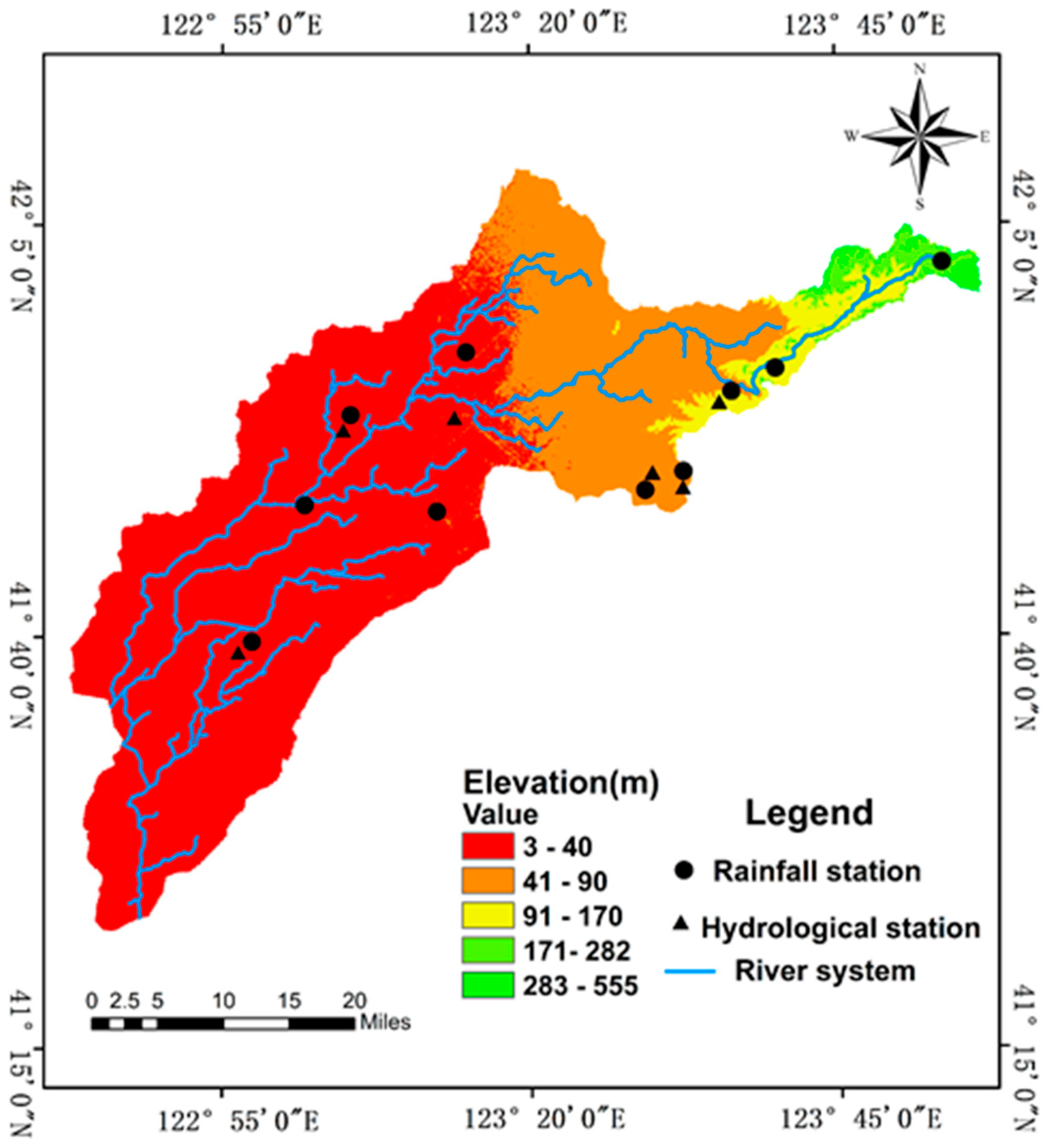
2.1. Study Area

Pu River (122°40′48″ E–123°56′32″ E, 41°21′53″ N–42°4′15″ N) has a total length of 205 km and a drainage area of 2610 km2. In Shenyang, the river length is 179.72 km, and the drainage area is 2248 km2. Pu River Basin belongs to the temperate continental monsoon climate, with an average annual rainfall of 647.4 mm, annual average evaporation of 1435.1 mm, and an annual average temperature of 8.2 °C. The hilly area is mainly distributed in the middle and upper reaches of the river, while the plain area is mainly distributed in the lower reaches of the river. The terrain of the Pu River Basin is shown in Figure 1.

2.2. Hydrological Data

There are ten rain stations and six hydrological stations in the basin, the earliest year for which data are available at all stations is 1975. In 2016, the construction of the Pu River ecological corridor and water system connection was started. Considering the consistency of flood data and the data integrity of all stations, we selected the rainfall-runoff data from 1975 to 2015 to analyze the model applicability before and after urbanization. Through analyzing the change in land use and watershed runoff, it was known that 1995 was a turning point in the process of urbanization [25]. In order to evaluate the application of the HEC-HMS model in different urbanization periods, seventeen typical flood events (Table 1) were screened out, among which ten flood events happened before 1995 and the others happened after 1995. Before 1995, six flood events were used for model calibration and 4 flood events for model validation. After 1995, four flood events were used for model calibration and three flood events for model validation.

3. Research Methods

3.1. Hydrological Model Methods Selection

HEC-HMS4.3 version consists of five parts to build the hydraulic model, which are the grid regions, the basin models, the meteorological models, the control specifications, and the time-series data. Among them, grid regions, basin models, and meteorological models are completed by HEC-geoHMS. Grid regions and basin models in vector form are imported into HEC-HMS. The Tyson polygon method is generally selected to determine the weight of sub-basins in meteorological modules and the distribution of rainfall across rainfall stations.

3.2. Loss Model

Considering the change in land use, the loss method selected is the SCS curve number. In this method, the net rainfall is estimated as a function of accumulated rainfall, land cover, land use, and previous humidity, as shown in Formula (1) [26].
P e = ( P I a ) 2 P I a + S
where Pe is effective rainfall; P is rainfall; Ia is an initial abstraction, assumed to be 20 percent of S; S is potential maximum retention after runoff begins, which can be estimated by Equation (2) [26].
S = 25400 254 C N C N
where CN is the runoff curve number.

3.3. Transform Model

The unit hydrograph model describes the relationship between direct runoff and rainfall. In this paper, the SCS unit hydrograph model is selected. Its core is a dimensionless unimodal unit hydrograph.
The delay time of the SCS unit hydrograph model can be estimated by the confluence time Tc, and the relationship is as follows:
T l a g = 0.6 T c
where Tlag and Tc are in minutes.
The time of concentration can be estimated based on basin characteristics including topography and the length of the reach by Kirpich’s formula [27].
T c = 0.0078 × ( L 0.07 S 0.385 )
where L is the reach length in feet, and S is the slope in (ft/ft).

3.4. Base Flow Model

In this paper, the exponential recession model is used to consider the effect of base flow on runoff. The parameters of the model include initial discharge Q 0 , recession constant k , and ratio to peak. The base flow model is given by:
Q t = Q 0 k t

3.5. Routing Model

The momentum equation and continuum equation in the Muskingum model are used to calculate the confluence evolution of the river. The water storage in the river is assumed to be a prism or a wedge, and the simplified finite difference method is used to approximate the formula as follows [28].
( I t 1 + I t 2 ) ( O t 1 + O t 2 ) = ( S t S t 1 Δ t )
where I t - 1 and I t are the vertical coordinates of the inflow process at time t − 1 and t of the reach, respectively; O t 1 and O t are the vertical coordinates of the outflow process at time t − 1 and t of the reach, respectively; S t 1 and S t are the water storage capacity of the reach at time t − 1 and t, respectively.
The Muskingum model defines the storage capacity as:
S t = K Q t + K X ( I t Q t ) = K [ X I t + ( 1 X ) Q t ]
In which the prism storage in the reach is K Q t , where K is a proportionality coefficient, and the volume of the wedge storage is equal to K X ( I t Q t ) , where X is a weighting factor having a range of 0 X 0.5 .

3.6. Accuracy Evaluation Methods

The performance of the model is mainly evaluated by PEV, PEPF, R2, and NSE.
The Percentage Error in Volume (PEV) accuracy evaluation formula is shown in Formula (8):
P E V = Q S Q 0 Q 0 × 100 %
In which Qs is the modeled flood volume, and Q0 is the observed flood volume.
The Percentage Error in Peak Flow (PEPF) accuracy evaluation formula is shown in Formula (9):
P E P F = q s q 0 q 0 × 100 %
where qs is the modeled value of peak discharge and q0 is the observed peak discharge.
The Coefficient of correlation (R2) and the Nash–Sutcliffe Efficiency (NSE) can be calculated by Equations (10) and (11), respectively.
R 2 = { i = 1 N ( O i O ¯ ) ( S i S ¯ ) [ i = 1 N ( O i O ¯ ) 2 ] 0.5 [ i = 1 N ( S i S ¯ ) 2 ] 0.5 } 2
N S E = 1 i = 1 N ( O i S i ) 2 i = 1 N ( O i O ¯ ) 2
where O i and S i represent the observed and the simulated flow, respectively; O ¯ and S ¯ denote the average values of the observed and the simulated flow, respectively.
The evaluation levels of each index are shown in Table 2 [29].

4. Results and Analysis
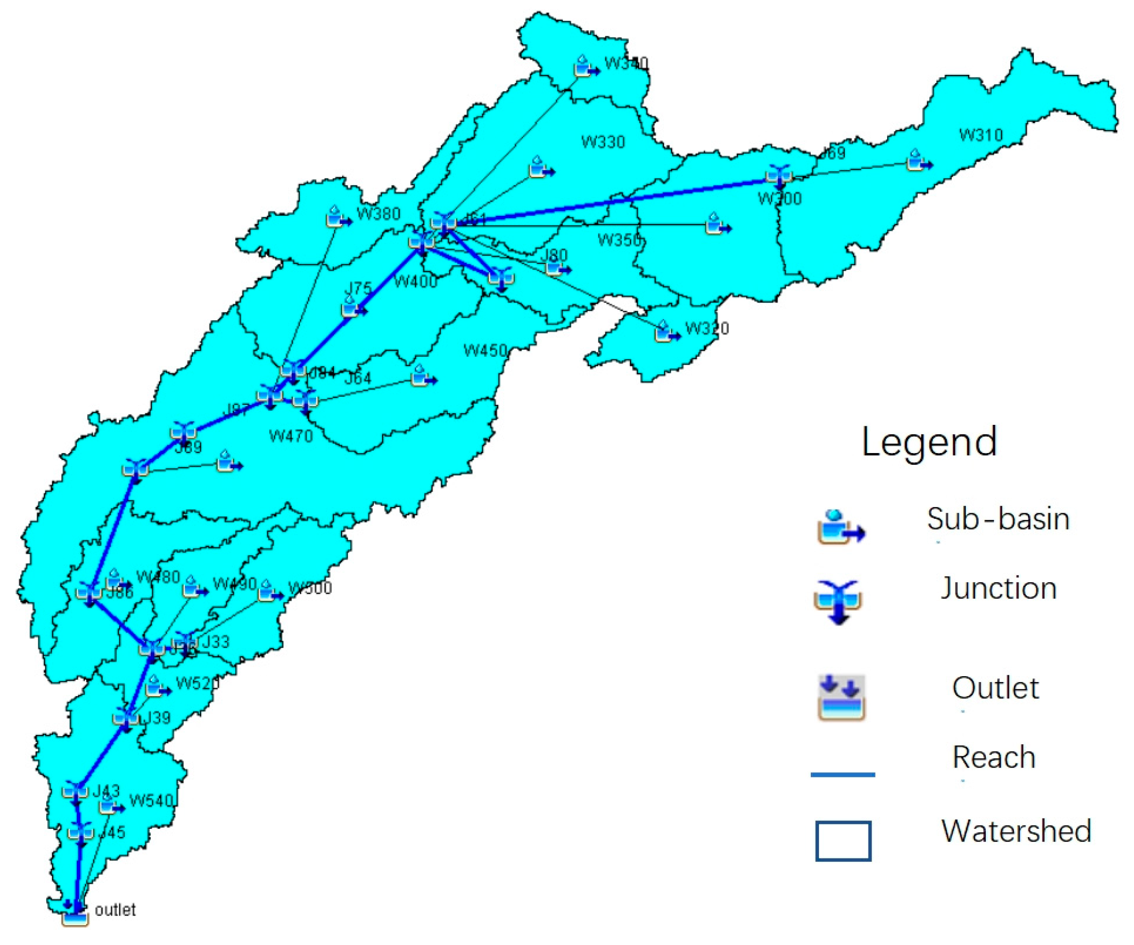
4.1. Model Building

According to the natural water division line, the sub-basins are generated. The HEC-geoHMS module will extract DEM (30 m × 30 m) of Pu River Basin to analyze the spatial unevenness of the underlying surface and the distribution of the river system, and through sink filling, flow direction calculation, flow accumulation calculation, water network extraction, and watershed boundary division, then a large watershed is divided into several sub-basins by natural water division line (Figure 2). The characteristic values of each sub-basin are also calculated by HEC-geoHMS (Table 3).

4.2. Determination of CN Value

As the most important parameter of the selected model method, CN value is an empirical parameter obtained by the Soil Protection Agency through experimental analysis of many small catchments in the United States, which is used to describe the relationship between rainfall and runoff in a natural state. Later, it was extended to urban watersheds to make the model predict approximate runoff. The major factors that determine CN are soil type, land use type, and hydrological conditions [26]. A higher CN value represents more runoff, and the CN value of the water body is 100 by default, which means that all rainfall is converted into runoff.
In this paper, remote sensing images of 1985, 1989, 1995, 2000, 2005, and 2010 in the study area were interpreted by the maximum likelihood method, and the soil texture was determined by superimposed FAO soil data. The soil impervious rate of each sub-basin was obtained, which was listed in Table 4.
It can be seen from Table 4 that 1995 was a turning point in the urbanization process. Before 1995, most of the impervious rates were lower than 10% while after 1995, the impervious rates increase deeply. In general, as the impervious area of the watershed increases, the CN value should increase. The soil type and land use type in Pu River Basin were treated by GIS and HEC-geoHMS to generate CNGrid [30]. Then, the weighted CN value will be used to present the CN of each sub-basin. The formula of weighted CN is as follows:
W C N = i = 1 n A i C N i i = 1 n A i
where WCN is the weighted Curve Number; Ai is the drainage area of subdivisions; CNi represents the CN initial value of subdivisions is calculated through CNGrid. It is worth noting that the CN value is a parameter with high sensitivity to estimate runoff error.
According to the urbanization process of Pu River Basin, two groups of parameters are calculated respectively (Table 5).

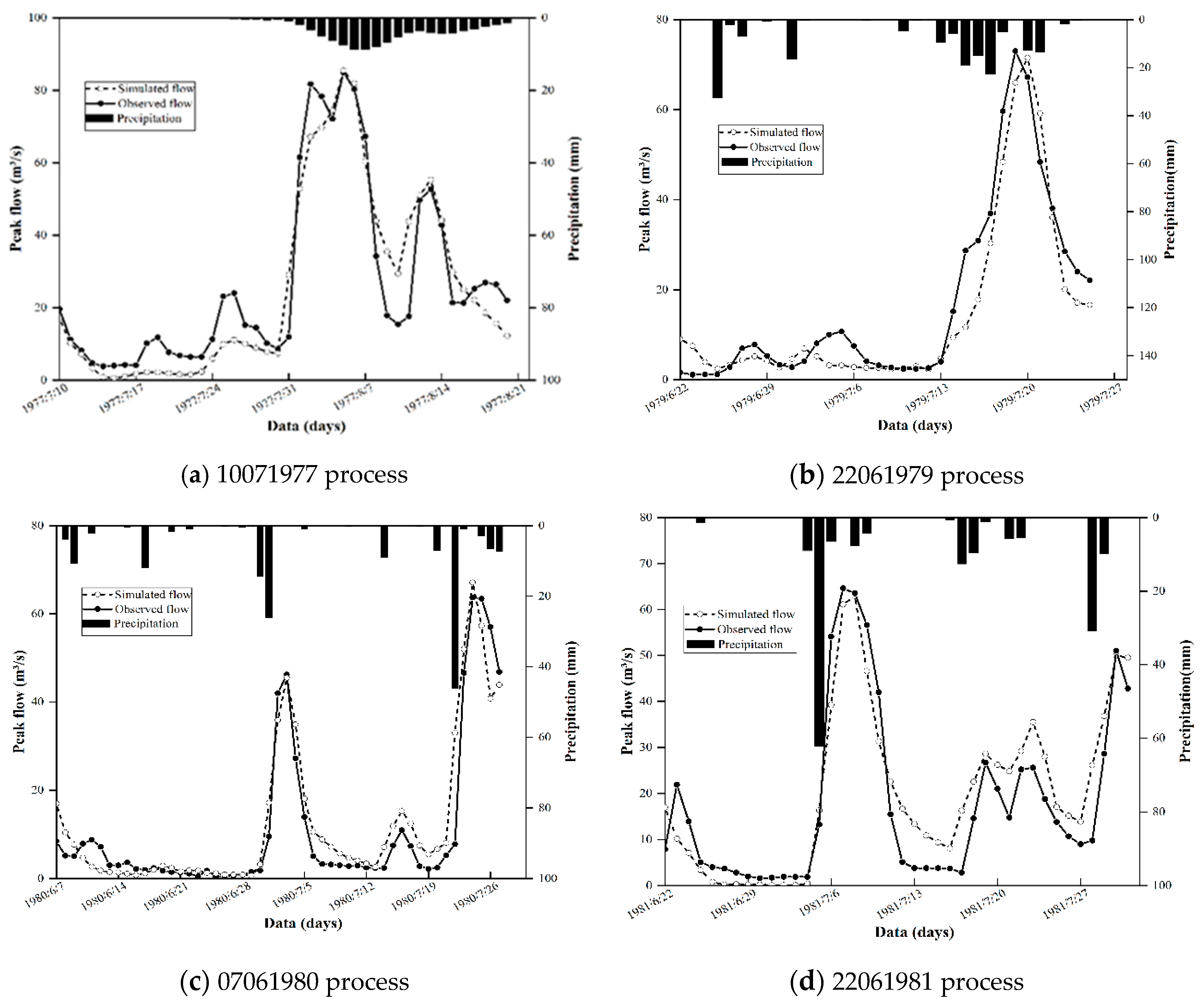
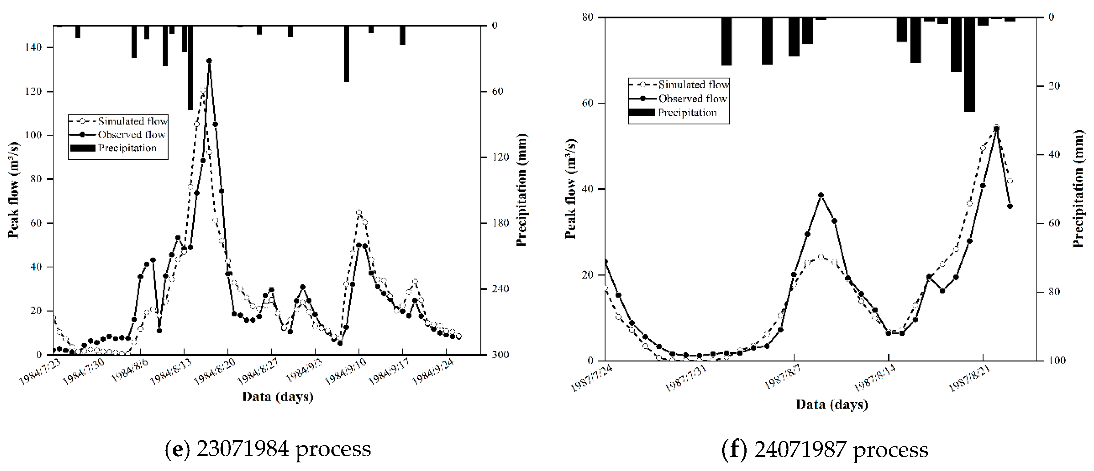
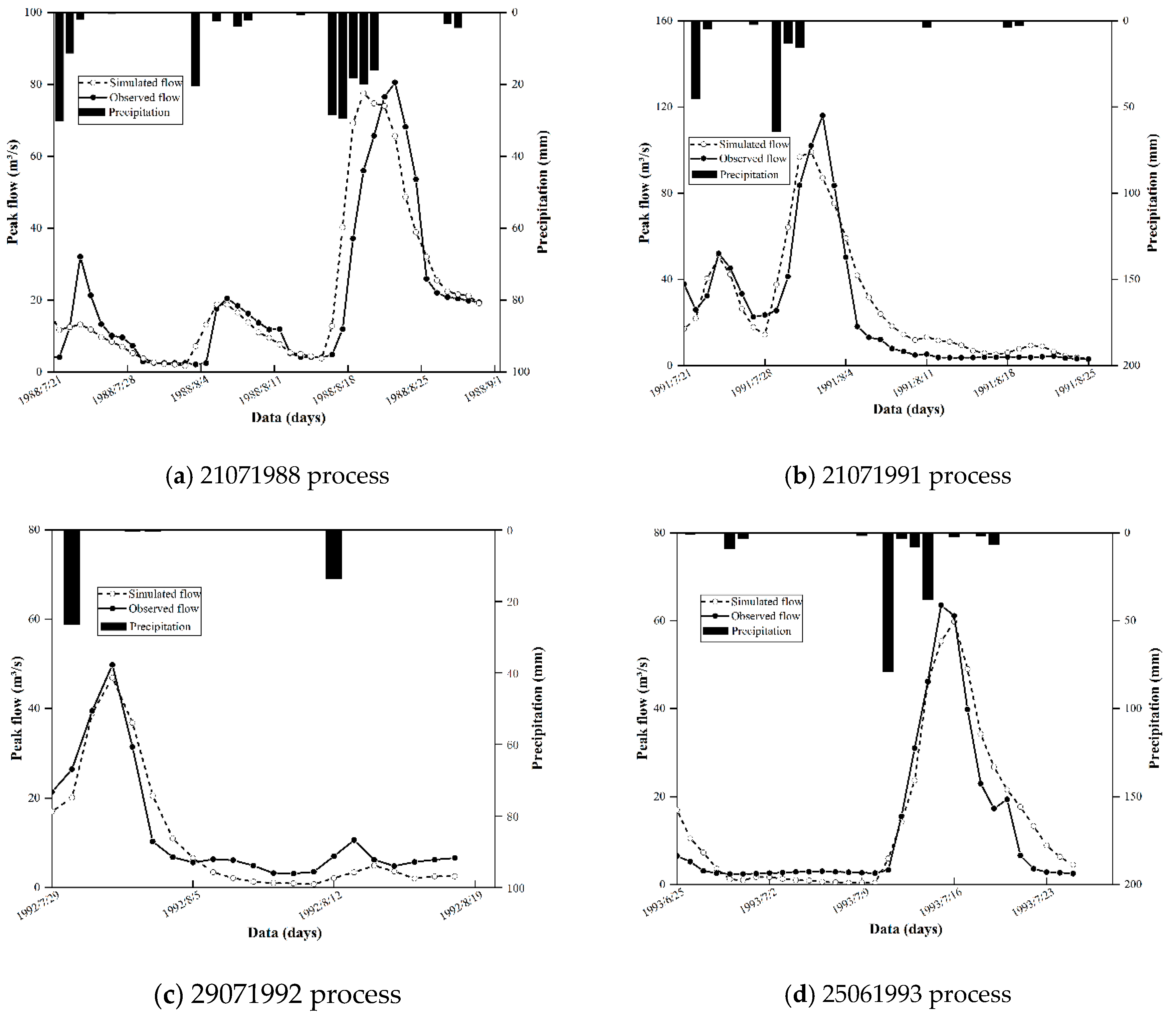
4.3. Model Calibration and Validation before Urbanization

Table 6 indicates the simulated and observed peak discharge and total runoff during the calibration and validation periods before urbanization. It is found that the simulated peak flow and volume are obviously close to the observed values. In both calibration and validation periods, the values of PEPF are lower than ±15%, the performance rating is very good. The values of PEV are lower than ±15%, which performance rating is good. To the NSE and R2, only one event’s value is lower than 0.75 while others are all bigger than 0.75, which performance is very good. All the evaluation results indicate the reliability of the model and parameters.
Figure 3 and Figure 4 are the comparison between the simulated process and the observed process in the calibration period and validation period respectively. It clearly indicates the model’s feasibility for flood simulation in the urbanization basin.

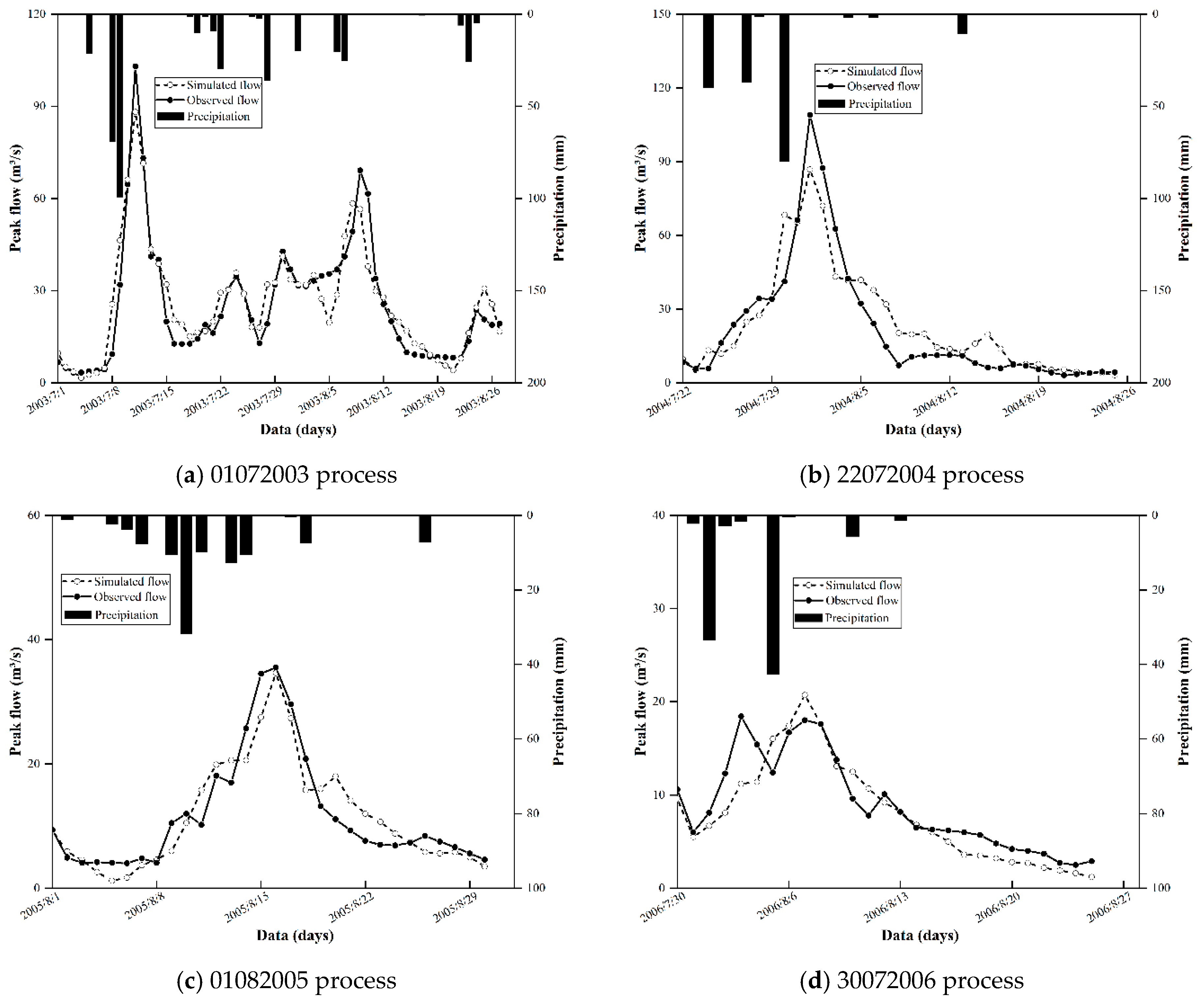
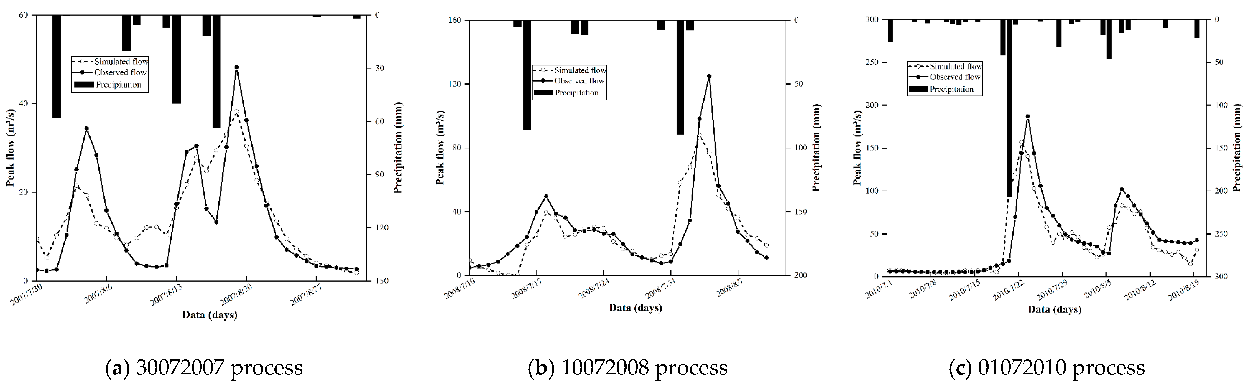
4.4. Model Calibration and Validation after Urbanization

Table 7 indicates the simulated and observed peak discharge and total runoff during the calibration and validation periods after urbanization. It is found that the values of PEPF in both calibration and validation periods are lower than ±30%, and the performance rating is good. The values of PEV are lower than ±10%, which performance rating is very good. To the NSE and R2, all the values are bigger than 0.65, which performance is good. The results indicate the reliability of the model and parameters.
Figure 5 and Figure 6 are the comparison between the simulated process and observed process in the calibration period and validation period respectively. It indicates the model’s feasibility for flood simulation in the urbanization basin.
While contrasting the evaluation results before and after urbanization, it can be seen that the simulation accuracy of the model before urbanization is higher than that after urbanization. The reason is that the loss method of the model is SCS, which is mainly affected by the topography, soil type, land use, and other basin factors. Especially in the river basin with a rapid urbanization process, the effect of model simulation will be decreased.

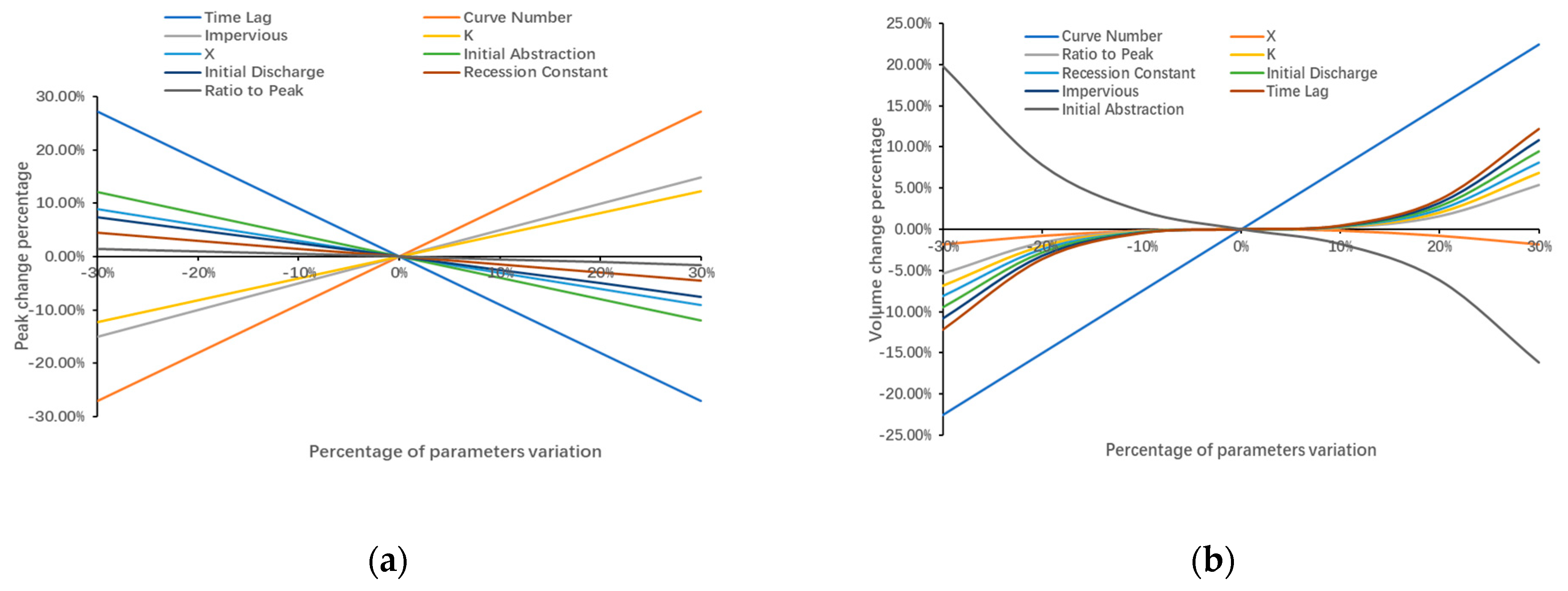
4.5. Parameters Sensitivity Analysis

A sensitivity analysis of the parameters is necessary for model calibration. It is mainly to adjust sensitivity parameters for manual calibration. The fluctuation range of the parameters is taken as ±30%, and the parameter value is changed at 5% as the interval point to simulate until the simulated flood curve is close to the observed curve [31]. Then, through the influence of the sensitivity of parameters on the peak flow (Figure 7a) and runoff (Figure 7b), the optimized parameters are determined to complete the calibration process of the model. In this paper, the HEC-HMS4.3 version was used to select the goal minimization, and the parameter optimization was carried out in combination with the root mean square error function.
The sensitivity of parameters is mainly judged by the magnitude of difference value increase or decrease. The larger the magnitude of the difference, the greater the sensitivity of the parameters. The intuitive performance on the graph is the absolute value of the tangent slope of the curve. The greater the tangent slope, the greater the sensitivity. Prioritize the adjustment of sensitive parameters and combine the simulated peak flow and runoff changes to quickly find parameters and optimize the model.
The sensitivity ranking of the parameters affecting the peak discharge is Time Lag > Curve Number > K > Impervious > Initial Abstraction > X > Recession Constant > Initial Discharge > Ratio to Peak. The sensitivity ranking of the parameters affecting the runoff is Curve Number > Initial Abstraction > Impervious > Time Lag > Recession Constant > Initial Discharge > Ratio to Peak > K > X. Comparing the size of the two sequences, it can be concluded that the main parameters that affect the model are curve number, initial abstraction, imperviousness, and time lag. In the actual process, the specific changes of peak discharge and runoff are combined to achieve precise parameter adjustment.

5. Conclusions

The study shows that the HEC-HMS model is suitable for the flood simulation of urbanization basins and can obtain good performance. Arcgis and HEC-geoHMS are used to process hydrological elements and calculate watershed characteristic values, laying a certain foundation for selecting appropriate methods for the construction of the HEC-HMS model. For parameter sensitivity analysis, manual parameter adjustment can be carried out quickly. In combination with HEC-HMS target minimization, model parameter adjustment can be carried out by mean-variance function, and appropriate parameters can be finally determined. Through parameter sensitivity analysis, it is concluded that the main parameters affecting the model are curve number, initial abstraction, imperviousness, and time lag.
Furthermore, it should be noted that the selection of loss of the SCS method should fully consider the changes in terrain, soil types, and land use. For the basins with rapid urbanization development, it needs an interval of time to calibrate the model. Based on the study of this paper, we can further deepen the analysis of hydrological phenomena in the urbanization basin, and study the impact of the change of underlying surface structure of urbanization on the process of flood yield and concentration. In the future research process, the reliability of the model should be further verified by comparing the changes of the main sensitive parameters in the years with rapid urbanization development.

Author Contributions

Conceptualization, J.Z.; methodology, J.Z. and X.Y.; software, X.Y.; validation, X.Y. and J.Z.; formal analysis, X.Y.; investigation, X.Y. and J.Z.; resources, J.Z.; data curation, X.Y.; writing—original draft preparation, X.Y.; writing—review and editing, J.Z.; visualization, X.Y.; supervision, X.Y. and J.Z.; project administration, J.Z. All authors have read and agreed to the published version of the manuscript.

Funding

This research received no external funding.

Data Availability Statement

All authors made sure that all data and materials support our published claims and comply with field standards.

Conflicts of Interest

The authors declare no conflict of interest.

References

  1. Sun, Z.; Zhu, X.; Pan, Y.; Liu, X. Progress and Prospect of flood disaster risk analysis. Disaster Sci. 2017, 32, 125–130. [Google Scholar]
  2. Li, J.; Wei, Z.; Liu, Y. Analysis of response degree of flood process to soil and water conservation project. J. Irrig. Drain. 2013, 32, 137–140. [Google Scholar]
  3. Wang, W.; Du, Y.; Chau, K.; Chen, H.; Liu, C.; Ma, Q.A. Comparison of BPNN, GMDH, and ARIMA for Monthly Rainfall Forecasting Based on Wavelet Packet Decomposition. Water 2021, 13, 2871. [Google Scholar] [CrossRef]
  4. Wang, W.-C.; Zhao, Y.-W.; Chau, K.-W.; Xu, D.-M.; Liu, C.-J. Improved flood forecasting using geomorphic unit hydrograph based on spatially distributed velocity field. J. Hydroinform. 2021, 23, 724–739. [Google Scholar] [CrossRef]
  5. Long, A.; Hao, W.; Yu, F.; Wang, J. Analysis on the theoretical basis of social water cycle II: Scientific problems and disciplinary frontiers. J. Water Conserv. 2011, 42, 505–513. [Google Scholar]
  6. Cuo, L.; Giambelluca, T.W.; Ziegler, A.D. Lumped parameter sensitivity analysis of a distributed hydrological model within tropical and temperate catchments. Hydrol. Process. 2011, 25, 2405–2421. [Google Scholar] [CrossRef]
  7. Wang, W.; Feng, Z.; Ma, M. Climate Changes and Hydrological Processes. Water 2022, 14, 3922. [Google Scholar] [CrossRef]
  8. Xin, J.; Qiong, C.; YanXiang, J. Influence of land use / cover data accuracy on hydrological process simulation. J. Irrig. Drain. 2018, 37, 108–115. [Google Scholar]
  9. Refsgaard, J.C.; Auken, E.; Bamberg, C.A.; Christensen, B.S.; Clausen, T.; Dalgaard, E.; Effersø, F.; Ernstsen, V.; Gertz, F.; Hansen, A.L.; et al. Nitrate reduction in geologically heterogeneous catchments—A framework for assessing the scale of predictive capability of hydrological models. Sci. Total Environ. 2014, 468, 1278–1288. [Google Scholar] [CrossRef]
  10. Sandu, M.-A.; Virsta, A. Applicability of mike she to simulate hydrology in argesel river catchment. Agric. Agric. Sci. Procedia 2015, 6, 517–524. [Google Scholar] [CrossRef] [Green Version]
  11. Hu, G.; Chen, X.; Yu, Z. Study on mountain torrent forecast in Chenjiang River Basin Based on HEC-HMS. J. Nat. Disasters 2017, 26, 147–155. [Google Scholar]
  12. Zheng, P.; Lin, Y.; Pan, W.; Deng, H. Study on flood return period of Bayi Reservoir Basin Based on HEC-HMS model. J. Ecol. 2013, 33, 1268–1275. [Google Scholar]
  13. Bo, W. Effects of Land Use/Cover Change on the Formation of Mountain Torrents in Gedong Watershed of Sanchuan River; Taiyuan University of Technology: Taiyuan, China, 2017. [Google Scholar]
  14. Yucel, I. Assessment of a flash flood event using different precipitation datasets. Nat. Hazards 2015, 79, 1889–1911. [Google Scholar] [CrossRef]
  15. Giannaros, C.; Dafis, S.; Stefanidis, S.; Giannaros, T.M.; Koletsis, I.; Oikonomou, C. Hydrometeorological analysis of a flash flood event in an ungauged Mediterranean watershed under an operational forecasting and monitoring context. Meteorol. Appl. 2022, 29, e2079. [Google Scholar] [CrossRef]
  16. Chang, L.; Chen, X.; Liu, C. Regional calibration of key parameters of HEC-HMS model in Jinjiang River Basin. S. N. Water Divers. Water Conserv. Sci. Technol. 2019, 3, 40–47. [Google Scholar]
  17. YanFu, K.; JianZhu, L.; QiuShuang, M. Construction of distributed HEC-HMS hydrological model and flood simulation in Zijingguan watershed. J. Irrig. Drain. 2019, 16, 108–115. [Google Scholar]
  18. Xing, Z.; Ma, M.; Wen, L.; Liu, C.; Lv, J.; Su, Z. Application of HEC-HMS model in mountain flood forecasting in data deficient areas. J. China Inst. Water Resour. Hydropower Res. 2020, 18, 54–61. [Google Scholar]
  19. Sardoii, E.R.; Rostami, N.; Sigaroudi, S.K.; Taheri, S. Calibration of loss estimation methods in HEC-HMS for simulation of surface runoff (Case Study: Amirkabir Dam Watershed, Iran). Adv. Environ. Biol. 2012, 6, 343–348. [Google Scholar]
  20. Tassew, B.G.; Belete, M.A.; Miegel, K. Application of HEC-HMS model for flow simulation in the Lake Tana basin: The case of Gilgel Abay catchment, upper Blue Nile basin, Ethiopia. Hydrology 2019, 6, 21. [Google Scholar] [CrossRef] [Green Version]
  21. Zelelew, D.G.; Melesse, A.M. Applicability of a spatially semi-distributed hydrological model for watershed scale runoff estimation in Northwest Ethiopia. Water 2018, 10, 923. [Google Scholar] [CrossRef] [Green Version]
  22. Du, J.; Cheng, L.; Zhang, Q.; Yang, Y.; Xu, W. Different flooding behaviors due to varied urbanization levels within river Basin: A case study from the Xiang river Basin, China. Int. J. Disaster Risk Sci. 2019, 10, 89–102. [Google Scholar] [CrossRef] [Green Version]
  23. Liu, S.; Zang, Z.; Wang, W.; Wu, Y. Spatial-temporal evolution of urban heat Island in Xi’an from 2006 to 2016. Phys. Chem. Earth 2019, 110, 185–194. [Google Scholar] [CrossRef]
  24. Bibi, T.S.; Kara, K.G. Evaluation of climate change, urbanization, and low-impact development practices on urban flooding. Heliyon 2023, 9, e12955. [Google Scholar] [CrossRef] [PubMed]
  25. Zhang, J.; Yu, X. Analysis of land use change and its influence on runoff in the Puhe River Basin. Environ. Sci. Pollut. Res. 2020, 28, 40116–40125. [Google Scholar] [CrossRef]
  26. Scs, U. Urban Hydrology for Small Watersheds, Technical Release no. 55 (TR-55); US Department of Agriculture, US Government Printing Office: Washington, DC, USA, 1986. [Google Scholar]
  27. Kirpich, Z. Time of concentration of small agricultural watersheds. Civ. Eng. 1940, 10, 362. [Google Scholar]
  28. McCarthy, G.T. The Unit Hydrograph and Flood Routing. In Proceedings of the Conference of North Atlantic Division; US Army Corps of Engineers: Washington, DC, USA, 1938; pp. 608–609. [Google Scholar]
  29. Moriasi, D.N.; Arnold, J.G.; Van Liew, M.W.; Bingner, R.L.; Harmel, R.D.; Veith, T.L. Model evaluation guidelines for systematic quantification of accuracy in watershed simulations. Trans. ASABE 2007, 50, 885–900. [Google Scholar] [CrossRef]
  30. Fleming, M.J.; Doan, J.H. HEC-GeoHMS Geospatial Hydrologic Modeling Extension User’s Manual; US Army Corps of Engineers: Washington, DC, USA, 2013. [Google Scholar]
  31. Ouédraogo, W.A.A.; Raude, J.M.; Gathenya, J.M. Continuous modeling of the Mkurumudzi River catchment in Kenya using the HEC-HMS conceptual model: Calibration, validation, model performance evaluation and sensitivity analysis. Hydrology 2018, 5, 44. [Google Scholar] [CrossRef] [Green Version]
Figure 1. General map of the Pu River Basin.
Water 15 02249 g001
Figure 2. HEC-HMS conceptual model for Pu River Basin.
Water 15 02249 g002
Figure 3. Comparison between simulation and observation in calibration period before urbanization.
Water 15 02249 g003aWater 15 02249 g003b
Figure 4. Comparison between simulation and observation in validation period before urbanization.
Water 15 02249 g004
Figure 5. Comparison between simulation and observation in calibration period after urbanization.
Water 15 02249 g005
Figure 6. Comparison between simulation and observation in validation period after urbanization.
Water 15 02249 g006
Figure 7. Percentage change against parameter percentage variation. (a) Change in peak. (b) Change in volume.
Water 15 02249 g007
Table 1. Statistics of floods.
Urbanization PeriodCalibrationValidation
Start DateEnd DateStart DateEnd Date
Before urbanization7 July 197720 August 197721 July 198831 August 1988
22 June 197925 July 197921 July 199124 August 1991
7 June 198027 July 198029 July 199218 August 1992
22 June 198131 July 198125 June 199325 July 1993
23 July 198427 September 1984
24 July 198723 August 1987
After urbanization1 July 200327 August 200330 July 200731 August 2007
22 July 200425 August 200410 July 200810 August 2008
1 August 200530 August 20051 July 201020 August 2010
30 July 200625 August 2006
Table 2. Evaluation standard and grade of hydrological model accuracy.
No.Performance RatingPEPF (%)PEV (%)NSER2
1Very good<±15<±100.75–10.75–1
2Good±15–±30±10–±150.65–0.750.65–0.75
3Satisfactory±30–±40±15–±250.50–0.650.50–0.65
4Unsatisfactory>±40>±25<0.50<0.50
Table 3. Characteristic values of each sub-basin in the study area.
Sub CodeArea
(km2)
Perimeter (km)Basin Slope (%)Main River Flow
Flow Length (m)Slope (m/m)
W300166.5387.84211.1319,9890.00070
W310225.87139.4815.2138,9160.00257
W32052.92954.8787.63--
W330223.22104.9929.8313,4210.00052
W34062.78662.11910.55--
W350121.4101.18111.5416,1170.00056
W38094.783103.27712.31--
W400180.8298.5135.9519,7180.00036
W450146.89104.22914.8322,7130.00048
W470434.45238.9477.3813,0480.00031
W480115.6596.6085.93--
W49072.74476.7915.9114,2100.00035
W50087.54981.3642.39--
W52070.72973.7426.2899860.00030
W540159.22103.0865.6573550.00027
Table 4. Statistics of impervious rate of sub-basins.
Sub CodeImpervious Rate
198519891995200020052010
W3100.41%0.50%16.10%23.54%37.42%19.75%
W3005.38%5.76%22.44%67.14%63.37%52.10%
W32058.45%62.99%84.37%93.40%91.40%85.64%
W3301.48%1.73%15.39%24.56%27.54%32.79%
W3402.79%3.19%6.11%11.70%15.79%18.66%
W3508.20%10.05%44.19%67.31%65.70%61.54%
W3804.09%8.63%11.33%23.27%27.86%37.47%
W4003.33%5.98%9.68%26.33%32.64%45.99%
W4505.50%6.22%18.41%35.08%49.36%57.48%
W4703.86%6.84%12.98%35.20%42.86%58.70%
W4804.69%5.22%10.81%26.79%35.51%56.35%
W4901.25%6.35%4.78%20.86%38.49%51.10%
W5001.75%5.87%7.94%24.46%37.35%60.99%
W5202.22%5.15%8.03%24.90%39.16%52.75%
W5402.23%4.66%10.09%20.96%32.51%54.31%
Table 5. Computed values of WCN in sub-basins.
Sub-BasinsW300W310W320W330W340W350W380W400
WCNbefore urbanization7176687882727567
after urbanization8491818595878985
Sub-basinsW450W470W480W490W500W520W540
WCNbefore urbanization77636666666466
after urbanization85818086898282
Table 6. Evaluation results before urbanization.
PeriodEventsPeak Discharge (m³/s)PEPFTotal Volume (mm)PEVNSER2
SO(%)SO(%)
Calibration77,70785.484.90.59106.08112.13−5.40.8770.888
79,62271.573−2.0593.03108−13.860.9060.919
80,60767.163.75.3461.754.2713.690.8950.902
81,62269.764.67.8977.5269.9210.870.8410.854
84,723120.7134−9.93173.06172.640.240.720.735
87,72455.1542.0444.6145.94−2.90.8740.912
Validation88,72177.580.5−3.7388.0984.114.730.7760.795
91,72199.2116−14.48100.7188.5413.750.870.882
92,72946.949.8−5.8222.1425.48−13.110.8860.917
93,62559.863.5−5.8343.1338.8710.960.9030.912
Notes: S and O respectively stand for simulated and observed values.
Table 7. Evaluation results after urbanization.
PeriodEventsPeak Discharge (m³/s)PEPFTotal Volume (mm)PEVNSER2
SO(%)SO(%)
Calibration0370188.1103−14.47151.99146.963.420.8750.879
0472286.8109−20.3783.2876.628.690.8470.858
0580134.635.5−2.5434.2634.61−1.010.8640.865
0673020.718.412.521.6123.67−8.070.7710.828
Validation0773038.248.2−20.7548.1846.363.930.7170.728
0871088125−29.686.4991.05−5.010.6870.689
10701157187−16.04194.98215.87−9.680.7640.777
Note: S and O respectively stand for simulated and observed values.
Disclaimer/Publisher’s Note: The statements, opinions and data contained in all publications are solely those of the individual author(s) and contributor(s) and not of MDPI and/or the editor(s). MDPI and/or the editor(s) disclaim responsibility for any injury to people or property resulting from any ideas, methods, instructions or products referred to in the content.

