Spatial Optimization of the Groundwater Quality Monitoring Network in the Kingdom of Bahrain

Abstract

Groundwater resource development, management, and planning essentially rely on their quantitative and qualitative monitoring. The information obtained from the monitoring networks of a given groundwater resource is used as a significant indicator for the status of that resource, and management schemes are subsequently made in order to develop and utilize this resource on a sustainable basis. In this study, the performance of the existing monitoring network of the quality of groundwater in Bahrain was evaluated and was spatially optimized using the geostatistical method of kriging. The estimation variance was used as a criterium in the design process, and variance reduction was used to measure the network performance. The process resulted in an increase in the number of observation points from 15 currently monitored wells to 91 wells, with 74% of these being augmented industrial and commercial wells that were to be self-reported to internalize the cost of groundwater management in their users. It is recommended that temporal optimization procedures for the groundwater level are conducted and that monitored groundwater quality data are stored in a dedicated groundwater management information system (MIS) along with the monitored data of groundwater levels and abstraction to effectively support the process of decision making for groundwater planning and management.

1. Introduction

Groundwater monitoring and data acquisition are pre-requisites for the effective management of groundwater resources. Monitoring makes the invisible groundwater visible. The main indicators used in groundwater development, management, and planning are groundwater levels and groundwater quality (e.g., salinity). These two “state variables” are used as indicators for the status of a groundwater resource and reflect the balance between its discharges (e.g., wells, springs, and evapotranspiration) and recharges (e.g., natural or artificial).

Groundwater monitoring is one of the most important tools in groundwater management. In the absence of monitoring, groundwater abstraction and waste disposal would take place without any safeguard for the groundwater resource, and the excessive use and contamination of an aquifer may continue unchecked for years until that groundwater resource is effectively deteriorated and lost. Therefore, the objective of monitoring is to reveal the changes taking place in the groundwater resource over time, and it thereby allows managers to introduce management interventions and restrictions to minimize the negative effect of these impacts. The continued collection of monitoring data allows groundwater managers to measure the effectiveness of these restrictions and their modifications if necessary. Moreover, the continuous monitoring of groundwater is essential to provide historical data that are essential for calibrating groundwater simulation models and that allow reliable simulations of future development and management scenarios [1]. Furthermore, the information obtained from monitoring groundwater resources can play a key role in increasing awareness among water users and stakeholders, and it thus facilitates the introduction of required groundwater demand management measures and aids their participation in groundwater management. In fact, as an awareness tool, the monitoring of groundwater can also lead to participatory self-monitoring, which helps reduce the costs to the water authorities [2].

The design and operation of any groundwater monitoring system needs to be carefully planned and designed so that relevant and useful information for management purposes can be obtained in a sustainable and “cost-effective” manner. In other words, monitoring networks need to be designed to have an optimal configuration, spatially and temporally, that would meet the groundwater management objectives by providing the required information more effectively and efficiently than any other configuration. Otherwise, there will be an inefficient use of the workforce and budget. Therefore, designing a monitoring network becomes an optimization exercise that aims at maximizing the usefulness of the information obtained from the network and the cost incurred in data collection within a set of constraints.

Data collection implies “use” and “worth” for those data, and usually the first data collected contain the most information and have the most worth. Hence, as more data are collected, their marginal worth decreases. However, their marginal cost does not. In this case, an optimal network design would have a configuration that either (1) has the maximum worth of a given budget or (2) has a design such that the marginal worth of the data is equal to their marginal cost. However, while the cost of data collection can be easily obtained for a given observation point in the monitoring network (i.e., the cost of well construction, installing equipment, and lab analysis), the worth of the data for this point is difficult to assess in economic terms. To overcome this difficulty in measuring data worth, surrogates to worth in the form of the measure of accuracy have been developed [3]. Examples of the measure of accuracy that are widely used as surrogates to data worth are the average and maximum errors within a network [4].

Groundwater observation networks, for the groundwater level and quality, are examples of the discontinuous sampling of variables having spatial continuity, i.e., a continuous non-discrete function. The measurement of these state variables at a number of selected points—that constitute the monitoring network—is used to interpolate the variable values in the whole aquifer domain at the unknown points (i.e., non-measurement points). The interpolation of the variable is typically produced in the form of a contour map from which spatial and temporal trends are concluded. One of the most widely applied methods for interpolation is the geostatistical suite of methods of which the most widely used method is kriging interpolation. These methods are used to compute the spatial distribution of the variable based on the existing observation points, and, more importantly, they determine the accuracy of the interpolated distribution. It is this last characteristic of the geostatistical methods that makes them widely applied in optimal network design [5]. The accuracy of the interpolation of the variables in the aquifer domain of interest, measured in the form of the variance in the estimation, is used as an indicator for the optimal sampling locations, and variance reduction is used as a measure of the network performance by computing the change in the estimation variance resulting from adding a fictitious (proposed) sample [6]. The average and the maximum variance within the network are used to dynamically improve the network sampling efficiency. The objective is to obtain a network, which provides a minimum variance estimate of the areal mean from a fixed number of sample stations [7].

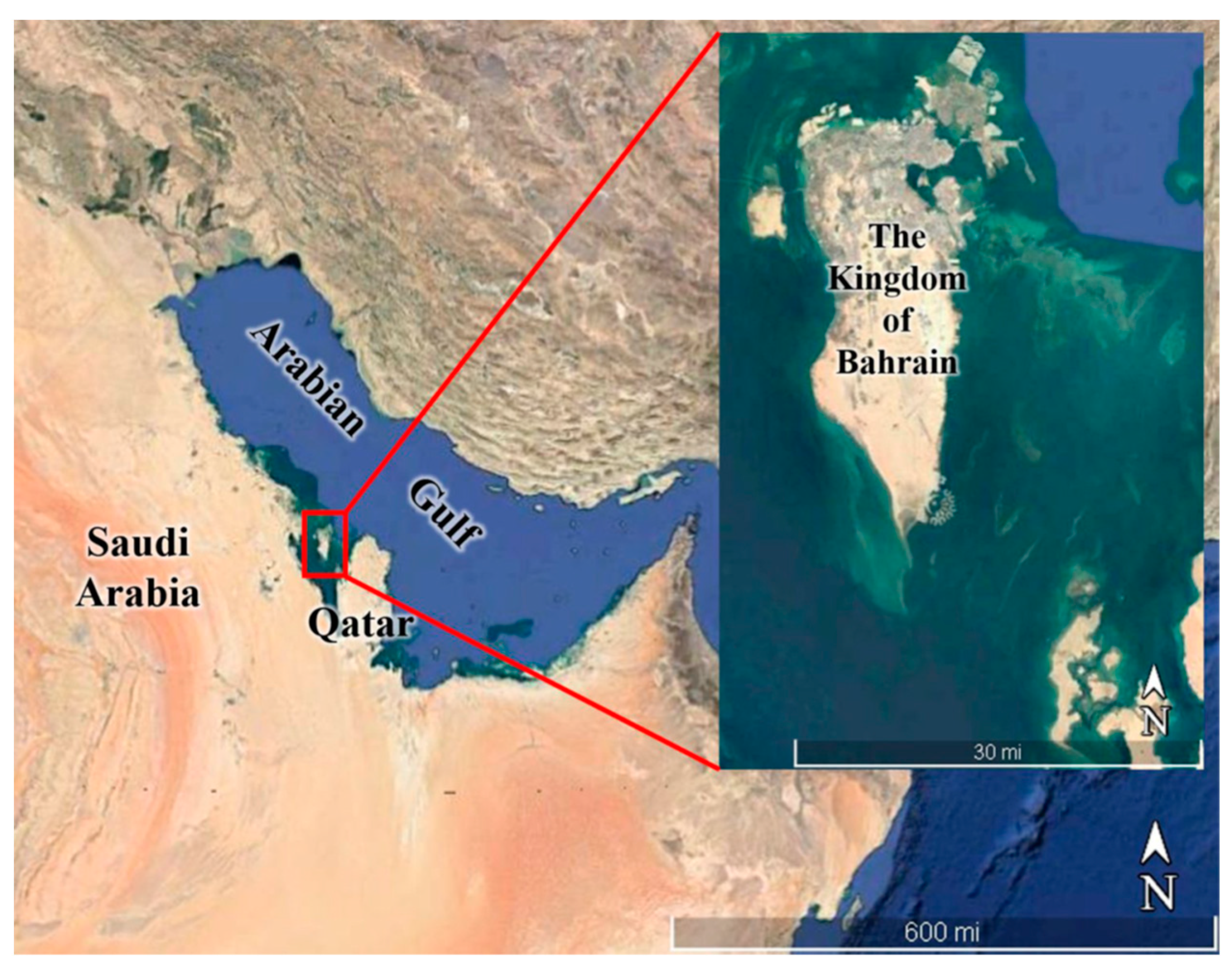
The Kingdom of Bahrain is a small island developing state (SIDS) located in the Arabian Gulf (Figure 1). Its groundwater is developed in the Dammam Formation, which forms a small part of the extensive regional aquifer system, termed the Eastern Arabian Aquifer, extending from central Saudi Arabia, where the main recharge area of the aquifer is located in the shores of the Arabian Gulf, including Bahrain. The recharging of the groundwater in Bahrain occurs through the lateral underflow from Eastern Saudi Arabia [8]. Locally, the groundwater system in Bahrain consists of two zones: the Alat aquifer zone and the Khobar aquifer zone. The Khobar aquifer zone is developed in highly fractured limestones and dolomites and is the principal aquifer in Bahrain. The aquifer provides the majority of groundwater abstraction and is the focus of this research.

Since the 1970s, heavy reliance on groundwater to meet the rapid water demands for the development and expansion of the agricultural and municipal sectors has led to its over-exploitation, which has resulted in a severe decline in groundwater levels, the cessation of natural spring flows, and the deterioration of groundwater quality due to the upward flow from the underlying brackish groundwater and the adjacent saline seawater. In response, the groundwater authorities in Bahrain have been making a number of management interventions on both the supply and demand sides to restore the groundwater, including reducing the reliance on the groundwater in the municipal water supply by increasing the desalination capacity, gradually substituting groundwater with the tertiary treated wastewater from agriculture and landscaping, prohibiting the industrial sector from using the Dammam aquifer’s water and directing it to the lower brackish and saline zones [9], and employing a number of irrigation water conservation and efficiency programs that aim at reducing the groundwater use in the agricultural sector. These efforts were successful in reducing the abstraction rates in 2019, causing them to be closer to the recommended safe yield rates. The monitoring of groundwater levels and quality as well as abstraction is becoming crucial to evaluate the effectiveness of groundwater restoration efforts. The availability of information on the groundwater response to these efforts is essential to support decision making in the process of groundwater planning and management in Bahrain.

The groundwater level monitoring program in Bahrain was established in the early 1980s when a dedicated monitoring network was developed for the Dammam aquifer, the principal aquifer in the kingdom. The establishment of the groundwater level network was based on the recommendations of a comprehensive hydrogeological study in Bahrain [8] aiming at the sustainable development and management of the groundwater system in the kingdom. However, regular groundwater quality monitoring was not performed for the Dammam aquifer until 2006. Prior to that, groundwater quality monitoring was carried out in the form of major decadal country-wide surveys in 1970 [10], 1978/1979 [8], 1991/92 [11], 2001/2002 [12], and 2014/2015 [13]. In 2006, the groundwater authority initiated a regular monitoring network of the groundwater quality of the main aquifer zone of the Dammam aquifer, termed the Khobar aquifer zone. The network started with about 44 observation points with samples being collected personally by the staff of the groundwater authority from produced private wells twice a year and being analyzed in government laboratories for salinity and major anions and cations. However, the number of observation points have started to decline gradually, reaching 15 wells in 2019. The decline is attributed to inadequate resources, the shortage of staff, inaccessibility to some wells, and the abandonment of some wells due to a salinity increase. Moreover, during the COVID-19 pandemic (starting in March 2020) monitoring stopped.

The objective of this study was to evaluate the effectiveness of the current groundwater quality monitoring system of the Khobar aquifer zone and to optimize its spatial distribution. The geostatistical optimization approach of kriging and GIS were employed to assess the adequacy of the existing monitoring system, to identify its main gaps, and to upgrade it to enhance its cost effectiveness under the constraints of production well availability, staff limitations, and aquifer limits to provide reliable information for groundwater planning and management. Moreover, it provides a number of recommendations to internalize the cost of groundwater management in groundwater users.

2. Materials and Methods

The methodology of upgrading groundwater quality monitoring network was based primarily on geostatistical methods supported by GIS analysis. Geostatistical methods (synonymous to kriging interpolations) are a group of statistical techniques used to evaluate and predict variations in space and time. Kriging is a local estimation technique of the best linear unbiased estimator (BLUE) for the unknown values of spatial and temporal variables [14]. Its mathematical concept was first introduced by D.K. Krige in 1951 to solve mining-related problem in South Africa, and the method was modified and introduced in the general form of kriging by Matheron in 1971 [15]. Geostatistical analysis, or kriging methods, based on variance, semi-variogram evaluations, and regionalized variable theories is used to compute spatial distributions, to determine the accuracies of those estimated distributions, and to obtain optimal sampling locations for monitoring groundwater. The methods have been applied in various disciplines, such as soil science, surface and sub-surface hydrology, meteorology, atmospheric science, and agriculture [5].

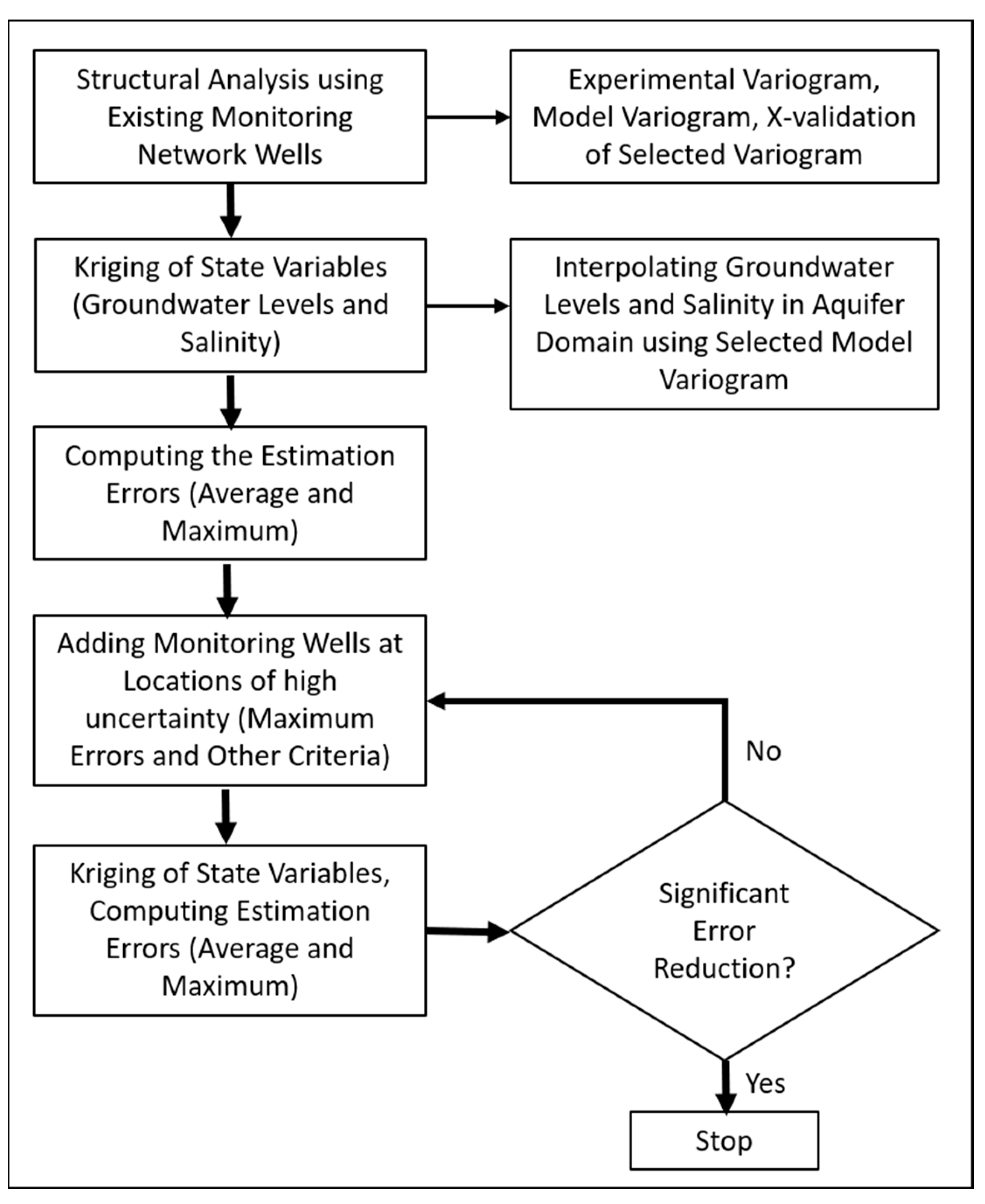
Variance-based approaches were established for the problem of groundwater monitoring network augmentation and upgrading [5] and have been used since the 1980s in upgrading groundwater monitoring networks, e.g., [16,17,18,19,20,21,22]. In this approach, the estimation variance and/or a weighted measure of estimation variance are used as criteria in the design process, and variance reduction is used as a measure of network performance. Variance reduction involves a methodical search for the number and locations of sampling sites that minimize the variance in estimation error of the state variable (e.g., water levels, salinity, or pollutant concentrations) of the aquifer. In practice, for groundwater quality monitoring, the search would be for existing operating wells that can be sampled. The search stops when adding new locations does not have a significant impact on reducing the variance, meaning that adding more observation points would not provide significant information (i.e., would not increase certainty of the variable being monitored). The methodology involved in implementing the variance reduction approach in evaluating and enhancing the effectiveness of groundwater quality monitoring network of the Khobar aquifer in Bahrain using Geostatistical Analyst Extension in ArcGIS software (Ver. 10.8) is illustrated in Figure 2. In detail, these procedures are as follows:

(1)

Data collection and preparation

This involved obtaining the location of the currently monitored wells (i.e., the X and Y coordinates of UTM projection and salinity values in 2019), which were treated as the existing networks of the aquifer that needed to be evaluated for adequacy. Moreover, the existing 15 wells were amended with the operating industrial wells produced from the Khobar aquifer zone. The chemical properties of the industrial wells tapping the Khobar aquifer zone are being analyzed frequently by their owners. However, these analyses are not reported to the groundwater authorities on a regular basis. The data of the currently monitored wells and the industrial wells were obtained from the files of the AEWRD and were verified to obtain their locations by plotting them in a GIS environment on a prepared base map of Bahrain as well as to obtain their operational conditions by interviewing the geotechnicians responsible for collecting the data from the wells.

(2)

Conducting a univariate statistical analysis for the data of the existing network

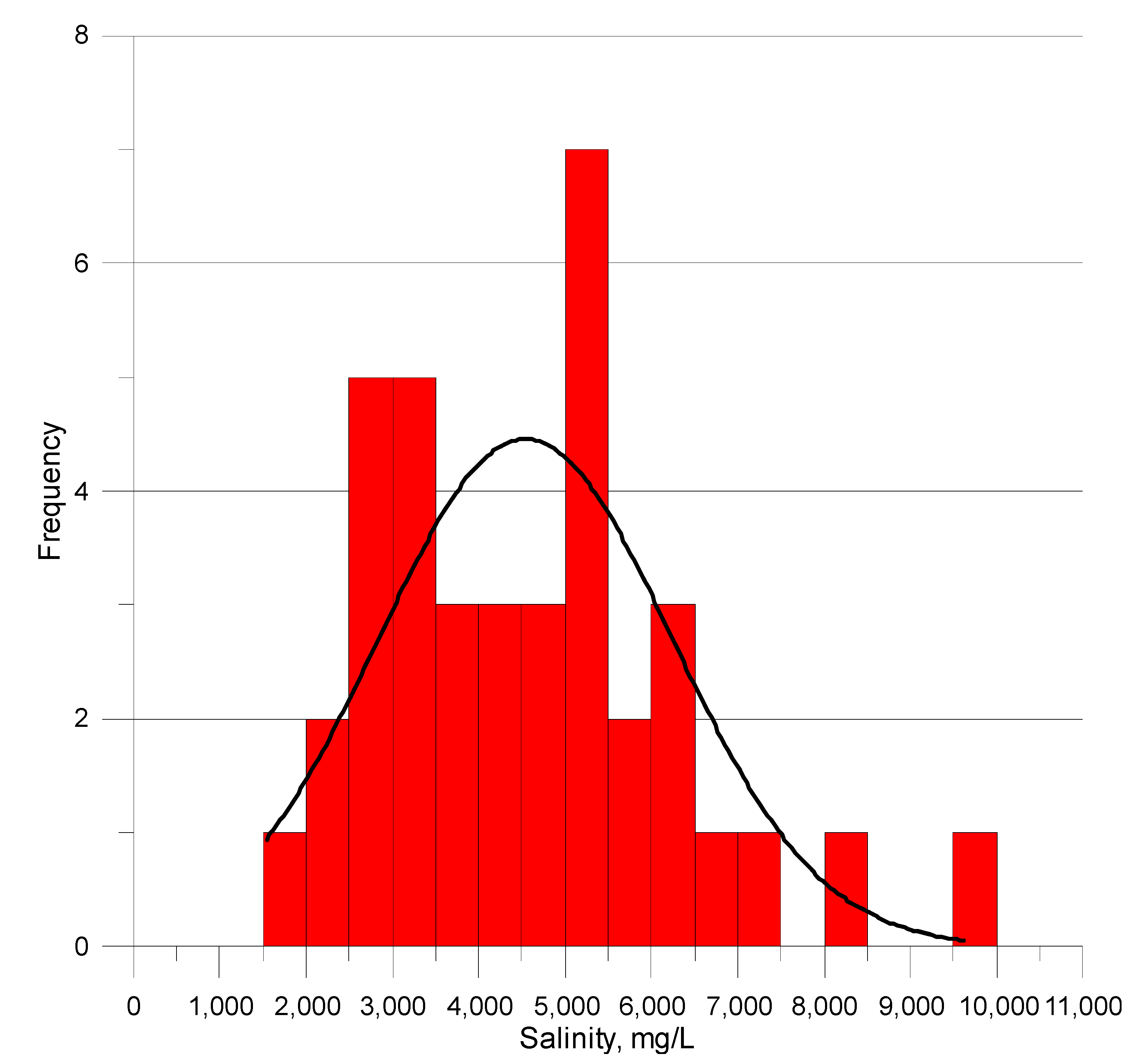
A classical univariate statistical analysis in GIS environment was performed on the existing monitoring network and industrial well data to determine the variables of frequency distribution and spreading patterns (i.e., mean, median, variance, minimum, maximum, skewness, and kurtosis). It should be noted that kriged estimation of the variables provides better estimation if the data used are normally distributed [23]. In the case the data exhibit a log-normal distribution, which is a typical behavior for many hydrogeological variables and parameters, then it is preferable to take the logarithm of the data before performing the geostatistical analysis and estimation [24,25]. This is performed because the structure of the variables is much better (i.e., the variogram shows a better correlation) if the log of the variables is used instead of its raw value [15].

(3)

Conducting structural analysis on the data of the regularly monitored wells from the AEWRD using the Geostatistical Analyst Extension of ArcGIS software

The structural analysis involved computing the experimental variogram, fitting the experimental variogram with a model variogram, and cross-validating the model variogram when estimating the value of the existing regularly monitored wells. In practical geostatistics, there are several methods that have been developed for the computation of the experimental variogram. Among these are the “classical” or traditional estimator [26], the Cressi–Hawkins estimator [27], the squared median of the absolute deviation (SMAD) estimator [28], and Omre estimator [29]. In this study, the classical estimator, which is widely used, was adopted to calculate the experimental variogram. The classical estimator equation is as follows:

$$\gamma \left(h\right)=\left[\frac{1}{2n\left(h\right)}\right]{\sum }_{i=1}^{n\left(h\right)}{\left[Z\left(x_i+h\right)-Z\left(x_i\right)\right]}^2$$

(1)

where the estimator γ(h) is the calculated experimental variogram; n(h) is the number of data pairs separated by the vector, or lag distance, h; and Z(x_i) is measured value of the state variable (i.e., salinity) at coordinate x_i.

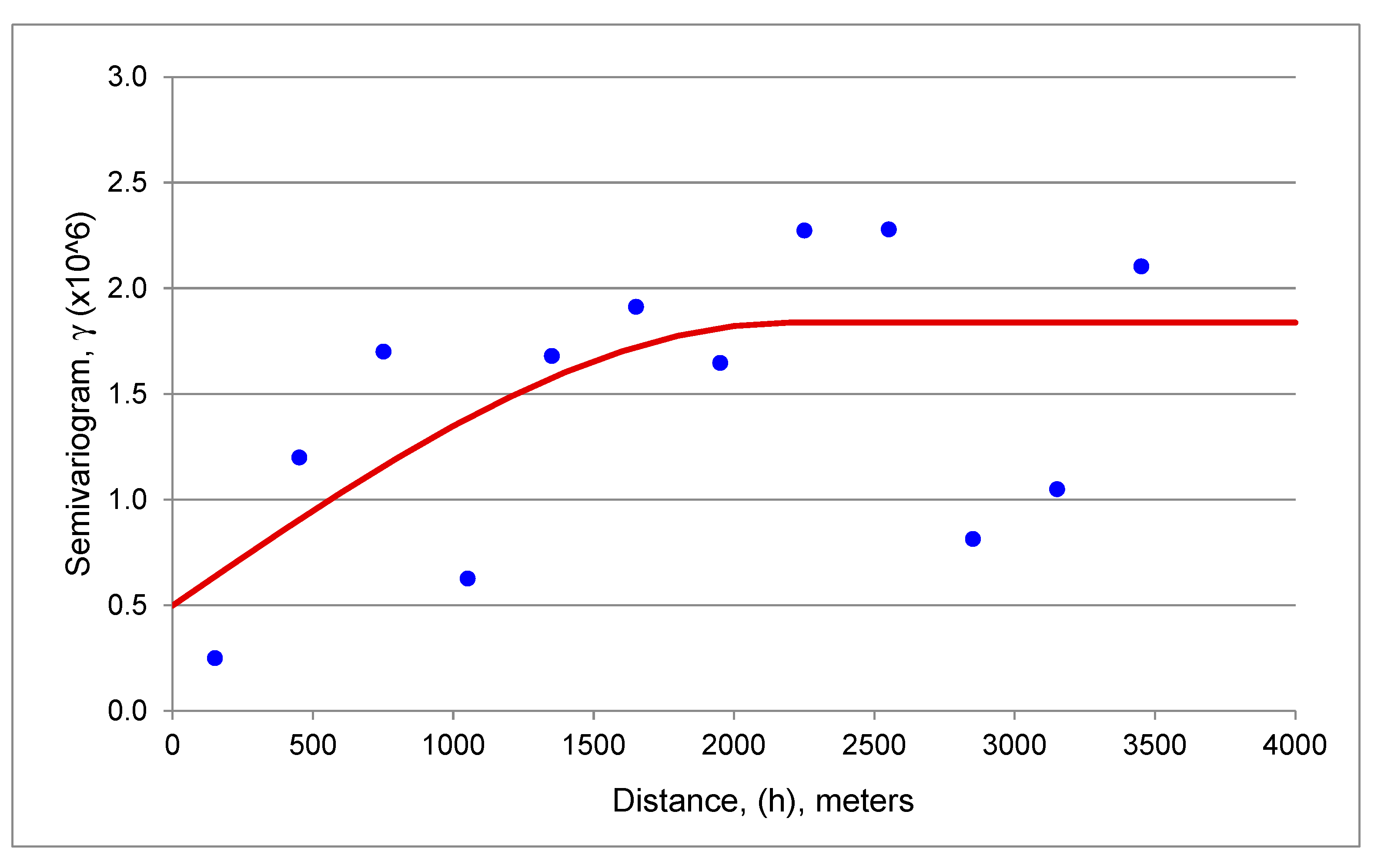
An appropriate theoretical model must be fitted to the computed experimental variogram in order to estimate the variable value at different locations in the domain of interest. Several theoretical mathematical models could be fitted to the experimental variogram, which include the spherical, exponential, power, Gaussian, and cubic models [30]. In this study, the spherical model, which is the most commonly used model, was found to be more applicable to the variable of salinity. The model exhibited a linear behavior at small separation distances near the origin, but it flattened out at larger distances and reached a sill limit, i.e., it was transitive, consisting of two separate functions with a discontinuity. The model equations are as follows [31]:

$$\begin{gathered} \gamma \left(h\right)=C_0+C\left[\frac{3h}{2a}-\frac{1}{2}{\left(\frac{h}{a}\right)}^3\right]forh<a \\ \gamma \left(h\right)=C_0+Cforh\ge a \end{gathered}$$

(2)

where a is the range of influence, C₀ is the nugget variance, and C₀ + C is the sill. C₀ and C represent the random and spatial components of variation, respectively.

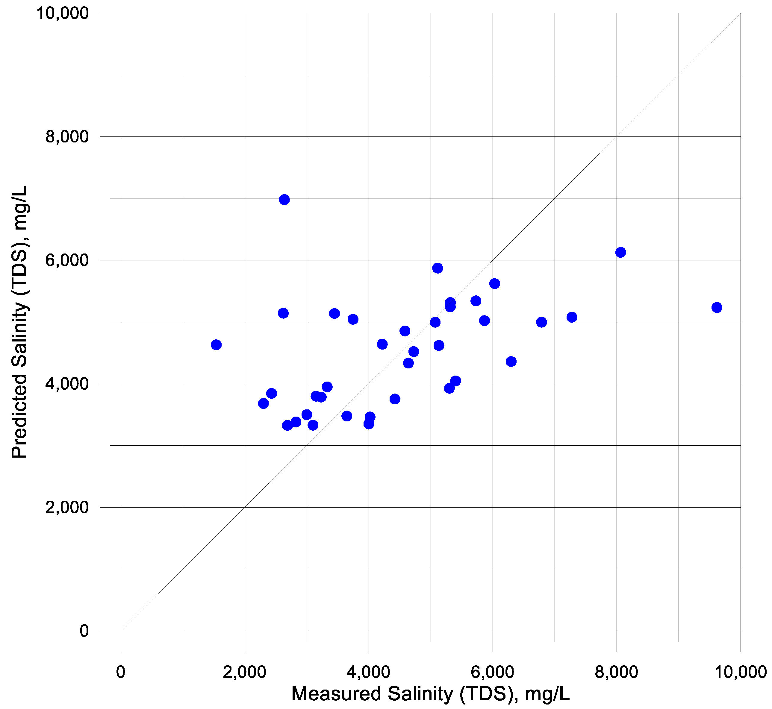
After fitting the model, cross-validation (or x-validation) was used to check the reliability and effectiveness of the calculated model variogram in estimating the variable field, i.e., groundwater salinity, in the aquifer. In x-validation, an estimation of each observed data point is made by utilizing the model variogram and the rest of the data set. This process is also called “jack-knifing”. At the end of this process, a comparison is made between the estimated values and the observed ones to indicate the goodness of the selected model.

(4)

Kriging the salinity using the existing observation points of the monitoring networks and the constructed model variogram using the Geostatistical Analyst Extension of ArcGIS Software

Kriging was used to estimate the values of the salinity at unknown locations in the aquifer. The regularly monitored AEWRD groundwater quality data and the structural variogram model (Equation (2)) were used in the estimation of the state variables’ function distribution in the aquifer. The kriging equations are as follows [30]:

$$\begin{gathered} \sum _{i=1}^n{\lambda }_0^j\gamma (x_i-x_j)+\gamma =\gamma \left(x_i-x_0\right)i=1,\dots n \\ \sum _{i=1}^n{\lambda }_0^i=1 \end{gathered}$$

(3)

where λ^j₀ is the weighting function of each point j to be used in the estimation of point x₀ and where γ(x_i − x_j) is the variogram value for the distance between x_i and x_j.

(5)

Calculating the error of kriging estimation using the Geostatistical Analyst Extension of ArcGIS Software

The error maps (maps of distribution of estimated uncertainty %) were useful in that they gave a realistic indication of the variability involved in contrast to kriged maps, which smoothed it out, and that they showed where the interpolated values deviated from the expected statistical structure, thus indicating the best position to place additional wells [32].

The variance in the error of estimation of point x₀ is given as

$${\sigma }_{x_0}^2={\sum }_{i=1}^n{\lambda }_0^i\gamma \left(x_i-x_0\right)+\mu$$

(4)

where μ is the Lagrange multiplier. The associated standard deviation of the estimation was generated for the domain in concern. The average error of the domain was computed, and the location of the maximum error was noted. Furthermore, a contour map for the distribution of the error involved in the estimation of the salinity of the Khobar aquifer zone was produced to indicate the location of high uncertainties. These maps were presented as uncertainty percentage, which is calculated by

$$Uncertainty\left(\%\right)=\frac{Error}{MaximumGridError}\times 100$$

(5)

(6)

Adding new locations of monitoring well(s) for the aquifer based on the maximum error and other criteria

The uncertainty maps were used to place new monitoring wells based on the maximum error found and were complemented by the existence of a production well. In other words, the existence of groundwater production wells (either government or private) was taken as the criteria for new site selections since augmenting salinity monitoring network is based on collecting samples from existing operating wells. The availability of production wells for augmenting groundwater salinity monitoring network was based on the AEWRD production wells database and was conducted using GIS. This step was performed by adding batches of wells.

(7)

Kriging groundwater salinity using both the regularly monitored wells and the newly added well(s) and calculating the associated error of estimation

Using the regularly monitored wells and the newly added ones, kriging was performed to estimate the values of the salinity at unknown locations in the aquifer zones. This was conducted using the same structural variogram model obtained in step (3) in GIS environment. This step was followed by calculating the associated error of the estimation in the form of the standard deviation, the average error of the domain, and the maximum error and by generating uncertainty distribution map for the monitoring network (similar to step 5).

(8)

Repeating steps 5 and 6 until no significant reduction in the error is observed

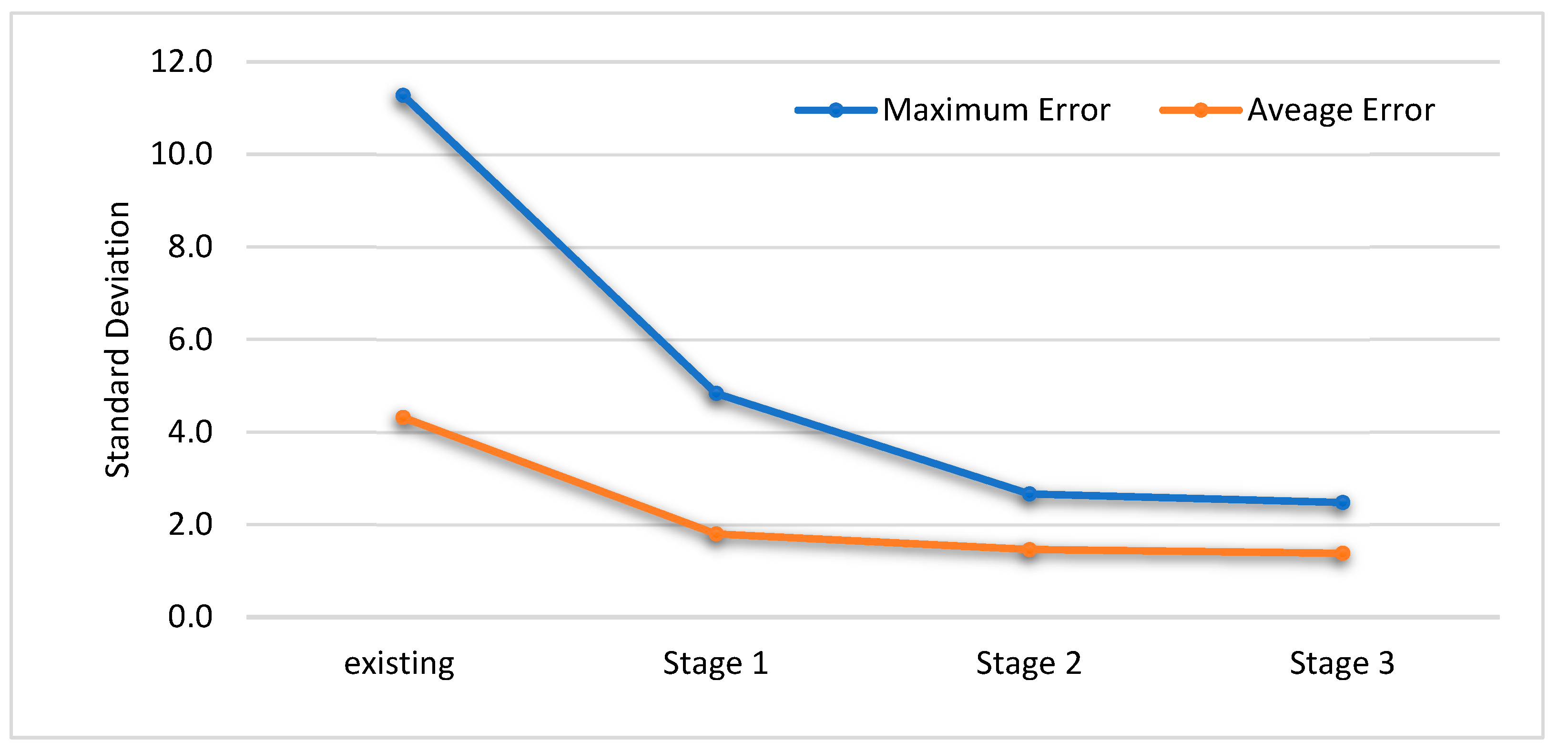
The addition of the wells, kriging them, and calculating the error involved in the estimation was repeated until the rate of improvement became relatively insignificant. While an increase in the sampling density will always decrease the involved errors and increase the sampling reliability, the rate of improvement will be different as more sampling points are added.

The objective was to obtain a “cost-effective” monitoring network that had a minimum variance estimate with a minimum number of sampling points. A plot of the number of wells and the change in the average error and maximum error provided an insight into the “worth of the additional data”, i.e., if obtaining more data by adding new wells would provide significant additional information on the state variable being monitored. Here, a managerial decision had to be made that took into account the available budget and workforce and the information obtained by adding more sampling points.

3. Results and Discussion

As indicated in the methodology section, the first step in analyzing, evaluating, and upgrading the existing monitoring networks of the Khobar aquifer zone was made by taking advantage of the industrial wells (23 wells), which are monitored on a regular basis with respect to their chemical properties by their owners. This increased the number of observation wells from 15 to 38. The following sections include the results of the analysis and evaluation of the quality monitoring network of the Khobar aquifer zone.

3.1. Statistical Analysis

The data statistics of the existing groundwater quality monitoring network (i.e., regularly monitored and the industrial wells) of the Khobar aquifer are summarized in

Table 1. Summary statistics of the groundwater salinity data of the Khobar aquifer zone.

Parameter	Value
N	38
Mean	4543
Median	4501
Variance	2,971,181
Standard Deviation	1724
Minimum	1540
Maximum	9616
Skewness	0.8
Kurtosis	0.8

. The frequency distribution of the quality data (salinity and TDS) of the Khobar aquifer zone is graphically illustrated in Figure 3, and its normal Q-Q plot is shown in Figure 4. The two figures indicate that the distribution of the Khobar data is close to normal, with a slight tendency to tail to the right. However, this does not warrant converting the data into logarithm values (doing so would cause the data to have a strongly skewed distribution to the right).

3.2. Structural Analysis

Figure 5 and Figure 6 display the experimental/fitted model variogram and the cross-validation results using the existing observation points of the groundwater quality monitoring network of the aquifer, respectively. The spherical model was found to best fit the variogram of the aquifer quality data, providing more satisfactory cross-validation results than the other models, and it was used in the following analysis.

3.3. Kriging and Kriging Error Analysis of Existing Network

Figure 7a depicts the uncertainty map resulting from kriging the TDS of the Khobar aquifer in Bahrain using the existing monitoring network data (regularly monitored and industrial wells in the Khobar aquifer zone) and the fitted spherical model. The main areas of concern are located in the northwestern and western areas, where the groundwater receives its recharge from the up-gradient parts of the aquifer in Saudi Arabia.

3.4. Upgrading the Existing Monitoring Network

The first step in enhancing the quality monitoring network of the aquifer was to augment the existing monitoring network with the commercial residential compounds. After this stage, it was important to look at the farmers’ wells that withdrew their water from the aquifer. The augmentation of the farmers’ wells was performed in two stages, each with nine wells obtained from the well database using GIS. Figure 7b–d illustrate the changes in the spatial uncertainty in these three steps, respectively.

Table 2. Maximum and average errors calculated for the estimation of water quality of the Khobar aquifer zone using the existing monitoring network and the various stages of adding new wells.

Stage	Maximum Grid Error	% Change in Maximum Error	Average Grid Error	% Change in Average Error
Existing wells (15 regular and 23 industrial wells)	11.27	-	4.32	-
Stage 1 (44 commercial residential compound wells)	4.83	57.12	1.80	58.35
Stage 2 (9 farmer wells—1)	2.66	44.91	1.46	18.75
Stage 3 (9 framer wells—2)	2.48	6.95	1.38	5.48

summarizes the results of the error analysis associated with these stages, while Figure 8 illustrates these results graphically. It can be clearly seen that adding the “commercial” residential compounds will significantly enhance the accuracy of the existing monitoring network (>50% change in accuracy). Similarly, the first stage of adding farmers’ wells will cause a relatively considerable enhancement of the accuracy. Therefore, it is highly recommended that these two stages are implemented and that the residential compounds (self-reported) and the first batch of the farmers’ wells (sample collection) are included in the monitoring network along with the industrial wells to augment the limited monitoring network of the principal aquifer in Bahrain. The third stage in collecting samples from the farmers’ wells will not change the accuracy values significantly, and, hence, adding more wells is not recommended.

4. Conclusions

The existing monitoring network of the quality of the Khobar aquifer, the main aquifer zone in the Kingdom of Bahrain, was spatially evaluated for its effectiveness in providing adequate information on the groundwater quality of the kingdom, and recommendations for upgrading and enhancing its cost-effectiveness in the planning and management process were made. The methodological approach involved implementing the variance reduction approach in evaluating and enhancing the effectiveness of the salinity monitoring network of the aquifer, based primarily on the geostatistical method of kriging coupled with GIS, and was constrained by the existence of production wells. In this method, the estimation variance is used as a criterium in the design process, and variance reduction is used to measure the network performance. Variance reduction involves a methodical search for the number and locations of the sampling sites that minimizes the variance in the estimation error of the groundwater salinity of the aquifer. The search stops when adding new locations does not have a significant impact on reducing the variance, meaning that adding more observation points would not provide significant information (i.e., would not increase the certainty of the monitored variable).

The current quality monitoring network of the Khobar aquifer, consisting of 15 wells, was augmented with an additional 23 industrial wells and was further augmented with 53 commercial residential compound wells to increase the total number of network observation wells to 91 wells. These additional industrial and commercial observation points are to be “self-reported”, which will internalize the cost of groundwater monitoring and management in their users and will reduce the cost of the operation of the network. A legislation requiring the certified lab analysis of the quality of the groundwater abstracted by these two sectors on a periodic basis is to be issued by the water authority. It is also recommended to include nine more farmers wells in the network to fill some areal gaps in the aquifer’s quality, which will require groundwater authority staff visits to collect the samples and analyses.

It is strongly recommended that monitored data are stored in a dedicated specialized groundwater management information system (MIS) along with the monitored data of groundwater levels and abstraction to effectively support the process of decision making for groundwater planning and management. Moreover, it is recommended that temporal optimization research, i.e., the frequency of sampling, is conducted for the groundwater monitoring system in Bahrain.