Abstract
Surface water bodies exhibit high dynamic variability on seasonal and interannual scales, and high spatiotemporal resolution water bodies extent data are crucial for studying surface water bodies’ evolution. Existing surface water bodies datasets are mainly based on optical data acquisition, which has the advantages of long temporal coverage and convenience but is susceptible to cloud contamination, leading to low spatiotemporal continuity. Although microwave remote sensing data are not affected by clouds, early SAR acquisition and short temporal coverage limit its use. Therefore, existing surface water bodies datasets face the problem of insufficient spatiotemporal resolution or low continuity. This research integrates Sentinel-2 optical data and Sentinel-1 Synthetic Aperture Radar (SAR) observations to reconstruct the surface water bodies dataset with a 6-day and 10-meter spatiotemporal resolution. Then, the proposed method introduces a spatiotemporal correlation model and predicts the land cover (water or land) of Sentinel-2 cloudy pixels, which improves the spatiotemporal continuity of the reconstructed surface water bodies dataset further. Based on the proposed method, we construct the Haihe River Water Dataset (HRWD) from 2016 to 2020 with a 6-day and 10-meter spatiotemporal resolution. Compared with the European Commission’s Joint Research Centre’s (JRC’s) Global Surface Water Explorer and Global Surface Water Extent Dataset (GSWED), the HRWD shows a rational accuracy (e.g., the overall accuracy of the HRWD is more than 93%) and a better spatiotemporal continuity, which provide an improved performance in identifying and monitoring surface water bodies in the Haihe River Basin. This indicates that the proposed method can improve the spatiotemporal continuity of surface water body mapping and meet the needs of accurate and long-term quantitative observation of the distribution of large-scale and high spatiotemporal continuity surface water bodies.
1. Introduction
Under the combined effects of natural mechanisms and human interference, the water cycle mechanisms in different basins exhibit different spatiotemporal evolution patterns. As an important element of the water cycle system, surface water bodies not only play a significant role in accurately describing the land water cycle but also greatly affect the water cycle as a whole [1]. High-precision and high-frequency spatiotemporal distribution information concerning surface water bodies can help hydrological and remote-sensing scientists gain new perspectives to understand and reveal global and regional water cycle mechanisms under the combined effects of climate change and strong human interference [2,3,4]. This requires the support of surface water bodies datasets with high spatiotemporal resolutions.
At present, remote-sensing-based methods for recognizing, extracting, and monitoring surface water bodies have achieved recognition at global and basin scales. The data sources are mainly divided into optical remote-sensing data and microwave remote-sensing data. Optical images mainly include the Moderate-resolution Imaging Spectroradiometer (MODIS) [5,6,7], Landsat [8,9,10], and Sentinel-2 [11,12,13], while microwave remote-sensing data mainly refer to Synthetic Aperture Radar (SAR) data, such as the Sentinel-1 [14,15,16] and ENVISAT-ASAR [17,18]. The water body extraction methods involved mainly fall into two categories: traditional algorithms (water body index and threshold methods) [19,20,21,22] and machine-learning classification algorithms (random forests, decision tree methods, and deep learning methods, etc.) [23,24,25]. Various methods have driven a series of water bodies datasets with different spatiotemporal coverage and spatiotemporal resolutions, ranging from small areas to the global scale, with spatial resolutions from 25 km to 10 m, temporal resolutions from one year to daily, and time scales from one year to more than a decade [26,27,28,29,30,31,32,33,34,35]. Although surface water body mapping has formed a system of multi-resolution, multi-temporal, and multi-classification criteria, various challenges still remain in high spatiotemporal continuity water body mapping, one of which is the low spatiotemporal characteristics of water bodies caused by cloud contamination. Although SAR is not affected by clouds, due to the difficulty in obtaining early SAR data, most water body mapping based on SAR focuses on small areas and short time scales [36,37]. Sentinel-1, as an emerging SAR data source, is easy to obtain but has a short time span, leaving it unable to support surface water body monitoring for a longer period before 2014.
To overcome the problem of cloud contamination, some researchers directly chose cloud-free scene images or cloud-free images synthesized from multi-temporal images, such as the Global Water Bodies Database (GLOWABO) dataset, which is a land surface water bodies product developed using global Landsat 7 annual composite satellite images with a spatial resolution of 14.25 m. However, it only has one phase in 2000 and cannot reveal the dynamic changes of land surface water bodies [35]. The Global Surface Water (GSW) dataset is a permanent land surface water bodies product with a spatial resolution of 30 m and a coverage range of 60° S to 80° N, produced using global multi-temporal Landsat satellite images from 2000 to 2012 [29]. The aforementioned methods can only partially overcome cloud contamination and cannot reveal the dynamic change characteristics of land surface water bodies. Considering the high variability of water bodies, some researchers have reconstructed the observed values of cloud-contaminated parts through time interpolation based on land cover categories after classification: water, ice, snow, land, and topographic shadows. For example, Pekel used a temporal sliding window in the post-classification of water bodies to eliminate or alleviate the impact of cloud contamination. In the sliding window, if the values before and after are water bodies, the observed value of the cloud-contaminated area is considered a water body. However, since seasonal water bodies have strong variability, cloud-free satellite observations must be carried out simultaneously with the dynamic changes of water, which leads to a decrease in the accuracy of seasonal water body mapping [33]. Han et al. used the image information of the previous and subsequent periods to solve cloud contamination and obtain continuous land surface water body ranges by interpolating and reconstructing the observed values of the cloud-contaminated parts [28]. Due to many issues with the data sources themselves and the problem of mixed pixels, the aforementioned methods cannot obtain truly high-frequency land surface water bodies datasets [38,39]. Furthermore, some researchers have eliminated the influence of cloud contamination by first reconstructing the land surface reflectance and then classifying and extracting water bodies. For example, Cheng et al. used a spatiotemporal Markov random field to guide cloud removal in cloud-free multi-temporal images by replacing similar pixels [40]. Lin proposed a patch information reconstruction-based method, which removed clouds by utilizing multi-temporal images of cloud-contaminated areas [41]. Chen implemented cloud removal based on a spatial and temporal weighted regression model, generating continuous cloud-free images [42]. The aforementioned methods typically use valid pixels adjacent to cloudy areas and data from other periods to predict the land surface reflectance in cloudy areas. When the changes in land surface reflectance are mainly caused by phenology, the constructed relationship is valid and the predicted values often have high accuracy. However, water bodies undergo dynamic changes, and when land cover changes suddenly cause variations in land surface reflectance, the constructed relationship is difficult to model and the results are often inaccurate [43]. Therefore, the approach of extracting water bodies based on the restoration of land surface reflectance under clouds may lead to a decrease in classification accuracy and greater uncertainty.
Another viable solution is to combine radar data and optical images. However, there are currently mainly low-resolution multi-source data integrated water body products, with few high spatiotemporal resolution water body products available. For example, the Global Inundation Extent from Multi-Satellites (GIEMS) dataset is a coarse-resolution (0.25° × 0.25°) land surface water bodies product synthesized from three types of data: passive microwave radiometer (SSM/I), active microwave backscatter coefficient, and AVHRR visible and near-infrared Normalized Difference Vegetation Index (NDVI) [32]. The Surface WAter Microwave Product Series (SWAMPS) dataset covers the period from 1992 to 2013, with a resolution of 25 km and a daily temporal resolution. The dataset was developed using three data sources: passive microwave sensors (SSM/I and SSMI/S), active microwave sensors (ERS, QuikSCAT, and ASCAT), and MODIS land cover products [44]. The aforementioned water body products have relatively low resolutions and can only reflect macroscopic changes in global land surface water bodies. Therefore, due to the inconsistency in the spatial resolution, temporal resolution, and time series length of multi-source data, there is currently no suitable fusion solution for producing high spatiotemporal continuity water bodies datasets.
In view of the shortcomings of existing water bodies datasets, this paper proposes a spatiotemporal correlation model to reconstruct water body information in cloud-contaminated images. This method uses the remote-sensing big data cloud platform (Google Earth Engine, GEE, Google Inc., Mountain View, CA, USA) for data acquisition and processing, and it integrates the all-weather advantage of active microwave Sentinel-1 SAR and the high-frequency characteristics of Sentinel-2 optical remote-sensing observations. By fully utilizing the spatiotemporal correlation and neighboring object similarity in multi-temporal SAR images, the water body information under clouds in optical images is reconstructed, thereby improving the spatiotemporal continuity of land surface water bodies datasets.
2. Research Area and Data
2.1. Research Area
The Haihe River Basin is located between 112° E and 120° E, and 35° N and 43° N. It borders the Bohai Bay to the east, the Taihang Mountains to the west, the Yellow River to the south, and the Mongolian Plateau to the north. The administrative divisions include most of the Beijing–Tianjin–Hebei region, the eastern part of Shanxi Province, the northern part of Henan Province, and the northeastern part of Shandong Province (Figure 1). The Haihe River Basin belongs to the temperate East Asian monsoon climate zone, with large inter-annual and intra-annual differences in precipitation and runoff, which often lead to drought and flood disasters, seriously restricting the development of the Beijing–Tianjin–Hebei urban agglomeration in the basin. At the same time, various production and living activities in the Beijing–Tianjin–Hebei urban agglomeration, one of the largest urban agglomerations in the world, are also strongly changing the water cycle mechanism in the Haihe River Basin, for example, rapid population expansion, economic model adjustments, and strong human interference factors such as the South-to-North Water Diversion Project. Therefore, this paper selects the Haihe River Basin as the research area to construct a high spatiotemporal continuity water bodies dataset, aiming to provide reference data for the planning and development of the Beijing–Tianjin–Hebei urban agglomeration.
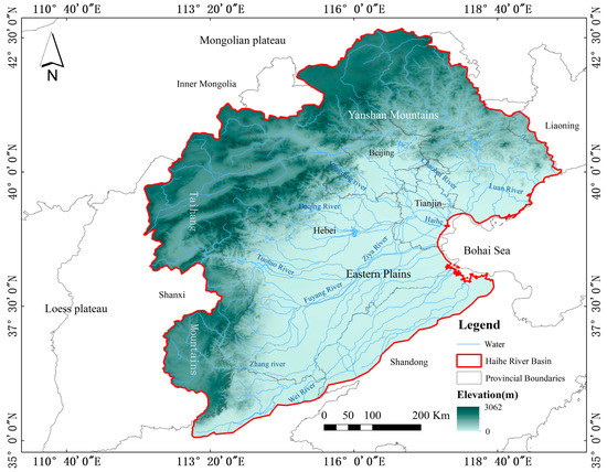
Figure 1.
Overview of water distribution in the Haihe River Basin.
2.2. Research Data
This study is based on the GEE platform and has acquired Sentinel-2 (S2) surface reflectance datasets and Sentinel-1 GRD (S1) datasets for the Haihe River Basin from January 2016 to December 2020. Sentinel-1 consists of two satellites, Sentinel-1A and Sentinel-1B, carrying a C-band SAR instrument, providing single-polarization (HH or VV) or dual-polarization (HH + VH or VV + VH) data products, with a spatial resolution of 10 m. Due to the dual constellation, the revisit period is 6 days. This study uses IW mode Sentinel-1 SAR GRD amplitude images, totaling 22,071 GRD images. The GEE officially pre-processes S1 data, mainly including updating orbital metadata using orbital files, eliminating GRD boundary noise, removing thermal noise, radiometric measurement calibration, and terrain correction (orthorectification). The global revisit period for S2 is 6 days, and the MultiSpectral Instrument (MSI) samples 13 spectral bands: 10 m visible and near-infrared, 20 m red-edge and SWIR, and 60 m spatial resolution atmospheric bands. The S2 surface reflectance dataset used in this study has been orthorectified to Level 2A. To eliminate the possible impact of clouds and fog, we filtered all the S2 images of the Haihe River Basin area (2016–2020) based on the cloud percentage, retaining images with less than 70% cloud cover. After cloud percentage filtering, a total of 34,390 S2 images were used for subsequent operations. We calculated the observation frequency of the two types of images in the Haihe River Basin at the pixel level, as shown in Figure 2. The total distribution observation frequency of Sentinel-1 and Sentinel-2 in the Haihe River Basin from 2016 to 2020 ranged from 107 to 4499, which can meet the water body mapping requirements of most areas in the Haihe River Basin with a six-day interval.
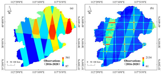
Figure 2.
Image observation frequency distribution map of the Haihe River Basin: (a) S1 observation frequency distribution map, and (b) S2 observation frequency distribution map.
The SRTM DEM data are used to generate slope data, which assist in removing mountain shadows from the water body results. The global water bodies dataset, referred to as the JRC, was generated by Pekel et al. at the European Commission’s Joint Research Centre (JRC) using Landsat 5, 7, and 8 imagery from 16 March 1984 to the present [33]. The JRC data products include water-body-related products such as water occurrence, seasonal surface water, permanent surface water, and maximum water body extent. In this study, the JRC’s water occurrence and maximum water body extent serve as auxiliary data, with water occurrence serving as prior knowledge for the sample point selection and maximum water body extent as a water body mask for the final result noise removal. The Global Surface Water Extent Dataset (GSWED) is a global surface water bodies product constructed by Han et al. based on the global water Normalized Difference Vegetation Index (NDVI) spatiotemporal parameter set of the MODIS from 2000 to 2020, with an 8-day temporal resolution and 250 m spatial resolution, and 863 observation counts [28]. This data product is used for the comparative analysis of the water bodies dataset constructed in this study. Table 1 summarizes all the data used in this study.

Table 1.
Research data.
3. Methods
In this paper, a Spatiotemporal Correlation Model (SCM) driven by Sentinel-1 SAR and Sentinel-2 data is proposed, aiming to integrate the advantages of SAR and optical satellite images to reconstruct water body information under clouds in optical images. (1) The method first constructs a basic water body database based on Sentinel-1 SAR images from 2016 to 2020, with a six-day interval. (2) Then, to address the cloud contamination issue in Sentinel-2 images, the method utilizes the multi-temporal spatiotemporal correlation and domain similarity of the Sentinel-1 SAR basic database to construct a spatiotemporal correlation model, which reconstructs water body information under clouds. (3) By combining surface water bodies extracted from both data types, the Haihe River Water Dataset (HRWD) with a 6-day, 10-meter high spatiotemporal resolution for the Haihe River Basin from 2016 to 2020 is achieved. The main steps include the construction of a basic water body database based on SAR data, the construction of a spatiotemporal correlation model, the reconstruction of invalid water body information in cloud-contaminated areas, and the related accuracy evaluation. The technical route is shown in Figure 3.
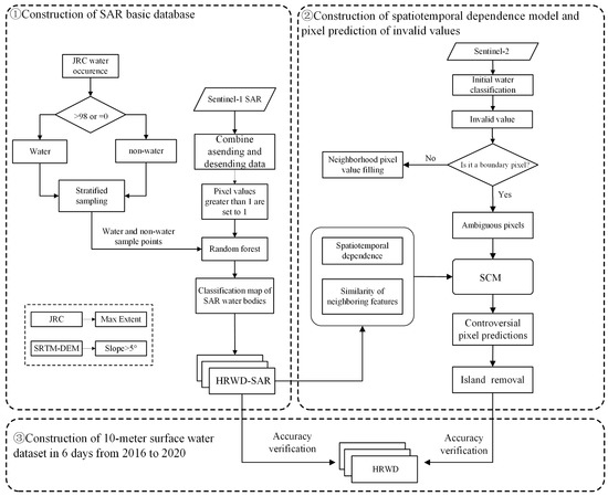
Figure 3.
Flow chart of the construction of a high spatiotemporal continuity water bodies dataset.
3.1. SAR Basic Database Construction
In this step, the study extracted water body information concerning the Haihe River Basin based on Sentinel-1 SAR images with a six-day interval from 2016 to 2020. The obtained multi-temporal water body distribution results served as prior knowledge for the subsequent cloud removal from the optical images. Firstly, the “Occurrence” band value of the JRC water occurrence product was used as the basis for determination, with values greater than 98 representing water bodies and 0 representing non-water bodies. A stratified sampling method was employed to randomly generate 500 sample points each for water bodies and non-water bodies. The corresponding time-phase SAR was used as the base map for manually modifying the sample points with incorrect category labels and obtaining accurate water bodies and non-water bodies sample points. Then, the SAR data to be classified were pre-processed, including the combination of ascending and descending tracks and normalization. This study combined ascending and descending tracks to reduce the impact of mountain shadows. Since the upper limit of radar reflectivity in SAR cannot be truly normalized, all the pixel values with radar reflectivity values greater than 1 were set to 1. Subsequently, using the random forest classifier encapsulated in the GEE platform, the training sample points and pre-processed SAR images were input to train the random forest model for the single-time-phase water body classification. Although combining ascending and descending SAR scenes can reduce some errors caused by radar shadowing or lingering, they cannot be completely eliminated [45,46]. Using optical sensors for surface water body detection has the issue of topographic shadowing, and many studies have shown that slope data can be used to remove the impact of topographic shadowing [28,31,47,48]. Therefore, this study used pixels with slopes greater than 5 degrees as a slope mask (water slope mask) to exclude areas where water bodies were unlikely to exist in steep regions. Masking the preliminary water extraction results with the JRC maximum water extent removed a large part of the interference from sand dunes and mountain shadows. Through the above post-processing, optimized SAR water body results were obtained. Finally, the same method was applied to classify and extract the Sentinel-1 images from January 2016 to December 2020, resulting in the Haihe River Water Dataset based on SAR, a surface water bodies database constructed using SAR (HRWD-SAR).
3.2. Spatiotemporal Correlation Model and Invalid Value Prediction
In this study, Sentinel-1 SAR and Sentinel-2 data were used for water body extraction, and the results of the two sensors were combined to obtain a high spatiotemporal water dataset with a six-day interval and a 10-meter spatial resolution. Due to the influence of atmospheric radiation, solar radiation, and uneven ground surface, water body extraction is highly susceptible to clouds and shadows, especially when dealing with long time series and large-scale images. In view of this, this study used the prior knowledge in the SAR basic database and constructed a spatiotemporal correlation model based on the spatiotemporal correlation of the multi-temporal water body distribution and the similarity of the pixel class labels to their neighboring pixels. This model was then used to reconstruct the water body information under clouds in the Sentinel-2 optical images. The detailed implementation process is shown in Figure 4.
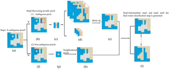
Figure 4.
Invalid value predicting process: (a) original target image; (b) retrieval of ambiguous pixels; (c) map block with an ambiguous pixel at the center; (d) extraction of multi-temporal map blocks from the SAR base data; (e) reconstruction of invalid pixel values using the pixel values; (f) retrieval of non-ambiguous pixels; (g) map block with a non-ambiguous pixel; (h) re-construction of invalid pixel values using neighboring pixel values; and (i) repeat steps 1 to 2 until all invalid values are reconstructed.
First, cloud and shadow detection was performed on the S2 target images, and the pixels affected by cloud contamination were considered invalid pixels, marked as −1, water bodies were marked as 1, and non-water bodies were marked as 0. Next, for the above category label results, a 3 × 3 sliding retrieval window was set, with nine pixels retrieved each time. When an invalid pixel value of −1 was detected, as shown in Figure 4a, the center pixel was judged to be a water body boundary pixel based on the pixel values in the eight directions surrounding the center pixel. When all eight pixels, excluding the center pixel, were either 0 (non-water) or 1 (water), as shown in Figure 4f, it could be determined that the center pixel was not a water body boundary pixel, i.e., the center pixel was not on the boundary line, and the invalid values in this part could be directly filled with the pixel values within the neighborhood. When the eight pixel values had all three values of −1, 0, and 1 at the same time, as shown in Figure 4b, the center pixel was suspected to be a boundary pixel, i.e., an ambiguous pixel. For ambiguous pixels, the neighborhood pixel window centered on the invalid value was extracted as a map block, as shown in Figure 4c. Based on the multi-temporal water body classification results of the basic database, the corresponding map blocks at the same location were extracted (Figure 4d), and then the index of the pixel neighborhood similarity () was calculated for each map block. For each time , the of the pixel compared to the target map block was defined as follows:
In this method, is a square spatial neighborhood consisting of all the valid pixels within the square window, with the center being ( itself is not included), and is the valid pixel adjacent to . In , is the pixel value of at time , and both and are valid pixels. The Euclidean distance between and is represented by . For each temporal phase , if and are the same, then = 1; otherwise, it is equal to 0. To ensure that the target pixel is predicted using pixels with similar neighborhoods, only pixels with values above a specific threshold are selected to predict the target pixel’s category. In this study, for each target pixel , the threshold of , Theta, was defined as follows:
where is a square spatial neighborhood consisting of all the valid pixels within the square window, is each valid pixel in , and is the similarity ratio value. In this study’s experiments, the value was set to 0.8, indicating that 80% of the valid pixels in the target pixel window were the same as the pixels in the reference pixel window. All the pixels with values greater than the threshold were selected, as shown in Figure 4h, and the weighted average of these pixels was calculated. The result was applied to the ambiguous pixels, generating an intermediate map corresponding to the aggregated time phase . For any , the value of the ambiguous pixel xi can be calculated as follows:
The above operations (Figure 4i) were repeated until all the invalid pixel values were filled. The final water classification results will be updated in the basic database. For areas where the prediction results have broken small patches leading to weak water connectivity, this study calculated the Water Occurrence () based on the generated multi-temporal water data and selected the water distribution range when the = 1, which is the minimum water range, to fill in the locally unconnected areas. The calculation of was performed as follows:
where indicates that the pixel is marked as water, n is the number of water observations, and N is the total number of good pixel observations in a specific time period.
Finally, the above steps were repeated to obtain the Haihe River Water Dataset (HRWD) with a 6-day, 10-meter resolution from 2016 to 2020.
4. Results
4.1. Accuracy Assessment of HRWD Surface Water Body Mapping
Since the water area accounts for a relatively low proportion of the total land surface area, randomly generating sample points within a large range of the river basin would result in only a very small number of points falling within the water area. Therefore, when generating verification sample points, in order to reduce the complexity of processing a large amount of data, we propose a verification sample point generation scheme for the minimum bounding rectangle area within the boundary range of the Haihe River Basin, supplemented by the JRC’s maximum extent water product as a spatial reference. This mainly includes four steps. First, the entire study area is divided into 100 small blocks. Second, 5000 sample points are randomly generated in each block, ensuring that the points are evenly distributed and random in space. Third, the sample points in the block area are screened, with two random points retained in the water area and one random point retained in the non-water area. Fourth, a visual inspection of the block samples is performed, and the sample points with mismatched labels between the sample point and the actual image feature are corrected using the corresponding high-resolution Google Earth imagery of the same date.
Following this approach, we select the true samples for the corresponding dates of the entire study area in the Haihe River Basin, resulting in a total of 1016 sample points, including 512 water samples and 504 land samples (Figure 5). This study selects five evaluation indicators to assess the accuracy of the HRWD. The accuracy indicators are shown in Table 2 and include the Overall Accuracy (OA), User Accuracy (UA), Producer Accuracy (PA), Commission Errors (CE), and Omission Errors (OE). Based on the above validation sample selection method and evaluation indicators, the surface water body results for different periods are validated. The average OA of the HRWD is 0.93, the average UA is 0.99, the average PA is 0.86, the average OE is 0.14, and the average CE is 0.01, meeting the accuracy requirements.
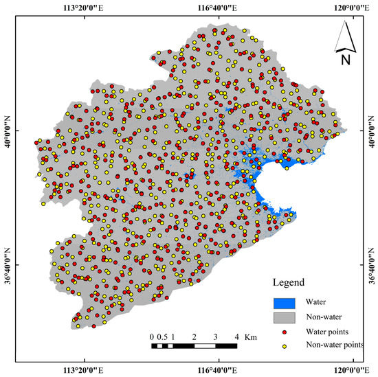
Figure 5.
Map of the sample points in the Haihe River Basin.
Table 2.
Evaluation indicators.
4.2. Spatiotemporal Correlation Model’s Recognition Capability for Cloud-Covered Areas
In the construction of the high spatiotemporal continuity water time series, the HRWD database uses the Haihe River Basin surface water bodies driven by S1 SAR data as a prior knowledge library and reconstructs the water distribution information in the cloud-contaminated parts of the S2 optical images through the spatiotemporal correlation model. This way, the two datasets are fused through the spatiotemporal correlation model to achieve a higher resolution and better spatiotemporal continuity water data time series construction. Apparently, the evaluation of the spatiotemporal correlation model’s reconstruction effect on the S2 cloud-contaminated water observations is directly related to the quality of the HRWD time series and the description accuracy of various water bodies in the Haihe River Basin. To evaluate the improvement in the spatiotemporal continuity of the HRWD data, we introduce the Intersection over Union (IoU) indicator to evaluate the cloud pixel water identification results. The IoU is the ratio of the intersection and union of the two water products, with values ranging from 0 to 1. When the IoU is 0, there is no intersection between the two water product distribution ranges; when the IoU is 1, the distribution ranges of the two water products completely overlap. The IoU calculation formula is as follows [49]:
In the formula, A represents the actual water distribution result, while B represents the reconstructed water distribution result.
In this study, the Miyun Reservoir is selected for experiments to test and quantitatively evaluate the effectiveness of the proposed method. In the simulation experiment, we simulate four different cloud cover conditions (10–20%, 20–30%, 30–50%, and 50–80%) on the original cloud-free water classification map (Figure 6(a1–a4)). Then, we reconstruct the cloud-affected classification map based on the spatiotemporal correlation model, with the specific results shown in Figure 6(b1–b4). The reconstructed water distribution results for the Miyun Reservoir are compared with the actual water distribution results extracted from the S2 water bodies (Figure 6(b1–b3)), and IoU statistics are performed (see Table 3). The results show that the average IoU for the SCM under different cloud coverages is 0.983, the average omission rate is 0.014, and the average commission rate is 0.015. As can be seen from the distribution results concerning the commission and omission errors in the water reconstruction maps shown in Figure 6(c1–c4), it is not difficult to see that the reconstruction results have reasonably reconstructed the cloud-affected pixels, with only minor differences from the actual S2 water distribution results at the edges. In terms of the statistical results, these differences are shown as omissions (blue) or commissions (red). The actual omission and commission errors relative to the actual water body statistics are part of the changes in the water body during its temporal evolution. This part is distributed along the edge of the Miyun Reservoir water body and is consistent with the water body’s evolution law and process, which is reasonable.
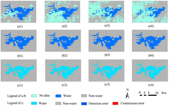
Figure 6.
Miyun cloud forecast results.
Table 3.
Evaluation of the reconstruction results of different cloud covers in Miyun.
4.3. HRWD’s Descriptive Capability for Typical Land Surface Water Bodies
In this study, manual interpretation is conducted on the Guanting and Miyun water areas in 2018, and the interpretation results are used as the ground truth for the comparison with the extraction results of this study (Figure 7). Figure 7 depicts the correlation between the area of the Guanting and Miyun water bodies in 2018 and the vectorized ground truth water body area in the form of a scatter plot. The results show that there is a strong relationship between the extracted water body area and the actual water body area in both study areas. Statistics show (Table 4) that the R2 values of the HRWD for Guanting and Miyun are 0.87 and 0.89, respectively, and the RMSE values are 2.39 and 5.01. Meanwhile, we also compare the existing mainstream water body products the JRC and GSWED with the vectorized ground truth of this study. The results show that the R2 values of the JRC are 0.44 and 0.62, respectively, and the RMSE values are 6.07 and 9.02; the R2 values of the GSWED are 0.30 and 0.53, respectively, and the RMSE values are 30.81 and 49.33. Overall, the HRWD time series can accurately depict the annual evolution of Guanting and Miyun in 2018, indicating that the water body extraction results of this study are reasonably accurate. Both the JRC and GSWED show deviations from the ground truth, mainly due to the relatively low temporal resolution of the JRC and the relatively low spatial resolution of the GSWED. In particular, the GSWED in early May and the JRC in September have significantly low values. This is because the data of the JRC, Landsat, only had one scene coverage image in September 2018, which was covered by a large amount of clouds, resulting in a severe loss of water information in the Miyun water area during that month. On May 9th, the GSWED’s water body recognition method was unable to extract complete water body distribution information, only extracting partial water body information.
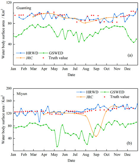
Figure 7.
Validation of the water bodies in the Haihe River Basin in 2018: (a) Guanting, and (b) Miyun.
Table 4.
R2 and RMSE between the truth value and HRWD, JRC, and GSWD, respectively.
4.4. Haihe River Basin Surface Water Bodies Changes
According to the literature, when the annual water occurrence is 0.25, the pixel is classified as an effective surface water body, forming the maximum water body extent; when the annual water occurrence is 0.75, the pixel is classified as a permanent water body extent, which is also the minimum water body extent; and when the annual water occurrence ranges from 0.25 to 0.75, the pixel is classified as a seasonal land surface water body [50,51]. Based on the HRWD, the maximum water body area, average water body area, permanent water body area, and seasonal water body area in the Haihe River Basin from 2016 to 2020 all show a decreasing trend (Figure 8). The maximum water body area is 9019.848 km2, and the minimum permanent water body area is 2908.338 km2. Comparing the areas of different water body types calculated based on the JRC and GSWED, it can be seen that the water body areas monitored by the HRWD and JRC are the closest, demonstrating the strength of the HRWD in revealing detailed spatial and temporal changes in surface water, identifying seasonal changes in surface water bodies and capturing more dynamic features of surface water bodies, implying its potential for long-term high-frequency analysis of the water environment.
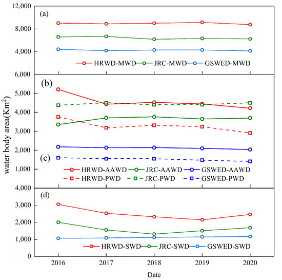
Figure 8.
Water body area distribution in the Haihe River Basin 2016–2020: (a) maximum water body area (MWD); (b) annual average water body area (AAWD); (c) permanent water body area (PWD); and (d) seasonal water body area (SWD).
5. Discussion
The work in Section 4 evaluated the accuracy of the HRWD and the ability of its spatiotemporal correlation model to identify water bodies in cloud-covered areas. Meanwhile, it demonstrated the capability of the HRWD to describe the temporal dimension of typical large water bodies in the Haihe River Basin, such as the Miyun and Guanting reservoirs. Compared to the JRC and GSWED, the HRWD better describes the evolution of the Miyun and Guanting reservoirs during 2018. The reason for this is the high spatiotemporal resolution of the HRWD, which leads to a better descriptive capability for typical water bodies. In addition, the spatiotemporal continuity of the HRWD has also been improved to varying degrees compared to the aforementioned two datasets, which endows the HRWD with the potential to better describe the details of the evolution process of land surface water bodies in the Haihe River Basin.
5.1. Spatiotemporal Characteristics Differences between the HRWD and JRC/SWED Land Surface Water Bodies Products
To demonstrate the advantages of the HRWD in terms of temporal and spatial resolution, this study compared three data products: HRWD, JRC, and GSWED. Due to the large research area involved, we chose to showcase the similarities and differences between the three types of water products by covering a range of water bodies as much as possible. Water bodies larger than 20 km2 account for over 80% of the surface water bodies in the Haihe River Basin, covering as many types of water bodies as possible (including typical water bodies such as linear rivers, mountainous areas, urban areas, reservoirs, etc.). Therefore, we chose a water range greater than 20 km2 to conduct research on three types of water products. Due to the lack of coverage in the source data and the influence of clouds and shadows, all three datasets have varying degrees of missing water body information, only extracting part of the actual water body information. The missing water body information leads to a lower actual water body area (Figure 9a). In months with more missing water body information, it can be seen that the JRC has the most severe missing data, with the water body area even being zero, such as in January and December every year, which indicates that the corresponding water bodies dataset has not been extracted. The GSWED has a significantly lower water body area than the HRWD and JRC in each month between 2016 and 2020, showing an obvious underestimation. On the one hand, this is due to the coarser resolution of the MODIS source data, which misses some small water body information; on the other hand, it is because the product does not effectively exclude the influences of clouds, ice, snow, and shadows from the MODIS. The water area of the HRWD and JRC land surface water bodies changes over time with high consistency, with a correlation of 0.823. However, the HRWD has a high temporal resolution of 6 days, which can reflect more water body information and show richer details in terms of water body changes (as shown in Figure 9a). To compare the relationship between the water body area and the time series of the three datasets, we synthesized the other two datasets on a monthly scale with the JRC as the reference, as shown in Figure 9b. It can be seen that the trend of the water body area changing over time is consistent for the three datasets. The HRWD is usually higher than the GSWED, and only in a few months in 2016, such as January, June, July, and August, the water body area is close to the GSWED. This is because of the lack of effective observation images in the Sentinel-1 images during these months, including severe ice and snow cover in January and partial missing observation images in June, July, and August, all of which can affect the acquisition of the true water body range, while the Sentinel-2’s images in June, July, and August are severely polluted by clouds. When the cloud coverage exceeds 80%, the effectiveness of our spatiotemporal correlation restoration is not ideal, which is also the reason why the water area of the HRWD during this time period is low and close to the GSWED. The highest correlation occurs between the HRWD and JRC, reaching 0.832. In addition, we counted the valid water body observation times for each water body pixel in the Haihe River Basin from 2016 to 2020 for the three data products and compared the valid observation characteristics of the three datasets using evaluation indicators such as the mean valid observation times, mode of valid observation times, and maximum valid observation times.
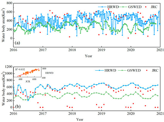
Figure 9.
Plots of the area of water bodies larger than 20 km2 in the Haihe River Basin with time series from 2016 to 2020: (a) 6-day temporal resolution (HRWD), 8-day temporal resolution (GSWED), and monthly scale JRC water body area with time series, and (b) monthly scale HRWD, GSWED, and JRC water body area with time series.
From the total valid observations per month for the six years from 2016 to 2020 (Figure 10a), the HRWD has the highest annual maximum valid observations of up to 26 times in 12 months, an annual mode of valid observations not less than 10 times, a maximum of 23 times, and an annual average observation times not less than 11 times, with a maximum of 17 times. In contrast, the JRC has the highest annual maximum valid observations of only 5 times in 12 months, an annual mode of valid observations of up to 5 times, with the lowest being 0 times, and an annual average observation times with a minimum of 0 times and a maximum not exceeding 4 times. The GSWED has the highest annual maximum valid observations of up to 20 times in 12 months, an annual mode of valid observations with a maximum of 20 times, a minimum of 1 time, and a majority of months with 1 time, such as April, May, June, and July; the lowest annual average observation times is 8 times, with a maximum not exceeding 13 times. The annual valid water body extraction times are all higher than the GSWED, with a maximum of up to 54 times. On a monthly scale, we counted the average monthly valid observation times for 2016–2020 (as shown in Figure 10b). The HRWD has the highest maximum valid observation times per month, higher than the GSWED and JRC data, with a maximum of up to 5 times, followed by the GSWED with a maximum of 4 times, while the JRC dataset, due to cloud contamination and longer revisit periods, has a maximum of 1 extraction per month, with no corresponding water body extraction data in certain months, such as January and December. The HRWD has a minimum monthly mode of valid observations of 3 times and a maximum of 5 times; the GSWED’s monthly mode of valid observations is mostly concentrated at 0 times, with a maximum of 4 times, indicating severe missing water body information in the GSWED; while the JRC’s monthly mode of valid observations is mostly concentrated at 1 time, with individual months at 0 times, such as January, February, November, and December. The HRWD has an average monthly valid observation times of 3, followed by the GSWED with a maximum of 3 times, and the JRC’s average monthly valid observation times are less than 1 time. The above analysis shows that the HRWD has higher valid observation times than the GWED and JRC, and it also has continuous high spatiotemporal characteristics.
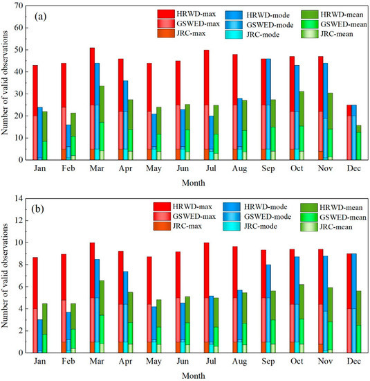
Figure 10.
Statistics concerning valid observation times for water bodies larger than 20 km2 in the Haihe River Basin from 2016 to 2020: (a) annual average total observation times, and (b) monthly average observation times.
5.2. Improvement of the HRWD’s Spatiotemporal Continuity
To further elaborate on the impact of differences in spatiotemporal resolution on the ability to describe the evolution of land surface water bodies, this study selected five typical water bodies in the Haihe River Basin for the HRWD, JRC, and GSWED (Figure 11): reservoirs (a), rivers (b), lakes (c), mountainous water bodies (d), and urban water bodies (e). The maximum water body extent and permanent water body extent of these five typical water bodies in 2020 were used to quantify the similarities and differences of the three water bodies datasets. As shown in Figure 12, the HRWD demonstrates a better description capability for different typical land surface water bodies, more completely describing the maximum annual range and permanent range of various water bodies; the JRC has a moderate ability to accurately describe different water bodies, showing a reasonable water body recognition capability close to that of HRWD; while the GSWED performs the worst, especially for small area water bodies or water bodies with poor continuity (such as mountainous water bodies, rivers, and fragmented wetland water bodies). The GSWED, affected by its 250 m resolution, has difficulty in effectively identifying these water bodies, resulting in a relatively common situation of under-detection. Although the HRWD and JRC data show relatively close water body spatial range description capabilities, a detailed comparison reveals that the JRC still has deficiencies in describing some detail parts. For example, in the Miyun Reservoir area (Figure 11a), the JRC still under-detects low-water occurrence water body areas (Figure 12a red box). This is obviously not due to the small spatial resolution differences between the two. We believe that the JRC’s lower temporal resolution and cloud effects during the rainy season led to the under-detection of this low-water occurrence. We further compared urban water bodies (Figure 12e), which generally have relatively stable water body ranges, meaning that urban water body ranges are fixed and have high flooding frequencies. Therefore, the JRC and HRWD show good consistency in recognizing urban water bodies. At the same time, as can be seen from Figure 12d,e, the JRC and HRWD still have consistent recognition capabilities for small and micro water bodies, which means that the change from 30 m to 10 m resolution does not cause a significant difference in the water body extraction and recognition results for this area. In summary, we infer that using the combination of S1 and S2 for higher water occurrence water body monitoring, as well as the all-weather capability of S1 SAR and the spatiotemporal correlation model for accurate identification of water bodies under cloudy conditions, are key to improving the HRWD’s ability to accurately recognize various water bodies.
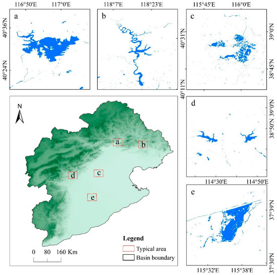
Figure 11.
Spatial distribution of five typical land surface water bodies: (a) reservoirs, (b) rivers, (c) lakes, (d) mountainous water bodies, and (e) urban water bodies.
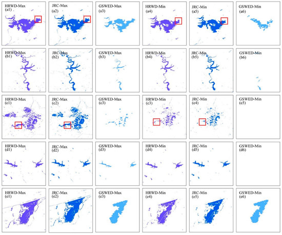
Figure 12.
Maximum annual water body extent (Max) and permanent water body extent (Min) for the HRWD, GSWED, and JRC in the five typical water bodies in the Haihe River Basin in 2020: res-ervoirs (a1–a6), rivers (b1–b6), lakes (c1–c6), mountainous water bodies (d1–d6), and urban water bodies (e1–e6). The red box indicates low-water occurrence water body areas.
The annual water occurrence maps from the JRC layers and the HRWD in Figure 13 were used to reveal the surface water spatiotemporal dynamics. First, the annual surface water count maps according to the JRC and HRWD maps were produced, respectively. For each typical water area, the JRC annual surface water count map was produced according to the 12 JRC monthly water history maps in that year, and the HRWD annual surface water count map was produced according to the 46 maps in that year. The surface water count was defined as the number of pixels labeled as water in the JRC monthly water history maps or the HRWD maps. Then, the water occurrence was defined by dividing the surface water count by the total number of valid observations.
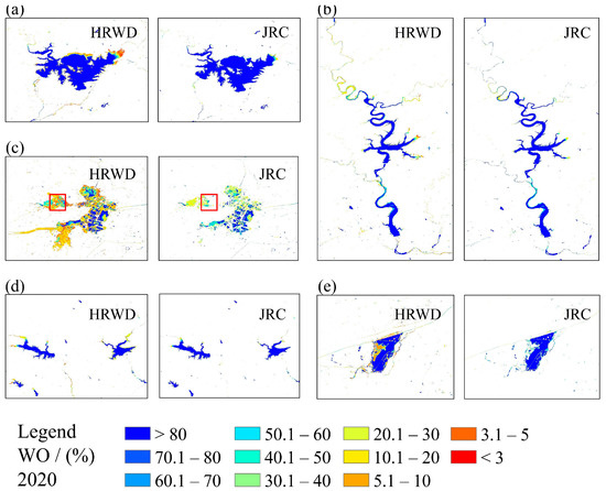
Figure 13.
(a–e) The annual water occurrence maps from the HRWD and JRC in five typical water bodies of the Haihe River Basin in 2020. The red box represents the comparison of the water occurrence maps of water flooding between HRWD and JRC at the same location.
Despite the relatively good consistency between the HRWD and JRC, significant differences can still be seen when comparing the water occurrence maps of the HRWD and JRC in Figure 13, particularly in the red rectangular box area in Figure 13c, where the JRC shows a higher water occurrence than the HRWD. This difference is due to the phenomenon of missing recognition in the JRC, which is related to the use of only optical data, as cloudy weather during the rainy and phenological seasons leads to the loss of water pixel information in the JRC products. In addition, many pixels in the JRC are “unobserved” in January, February, March, and December, which can lead to overestimation of the frequency of water flooding in the JRC. In contrast, the HRWD integrates optical and SAR data to recognize water body information under clouds, excluding “no observed values” and missing identified pixels. Therefore, the effective observed values of all the pixels in all the typical water bodies predicted by the HRWD in the time series are equal to 46. In the HRWD water occurrence map, the impact of the spatiotemporal distribution of “no observation” and “missing recognition pixels” can be reduced, which can truly reflect the evolution information of the surface water bodies. This also indicates that the HRWD surface water bodies constructed in this article are more capable of monitoring higher frequency water body information.
In summary, through the comparative analysis of different water body types, we preliminarily confirmed that the land surface water bodies identification accuracy of the HRWD is reasonable. Specifically, both the HRWD and JRC can provide accurate and similar descriptions and identifications of water bodies with different spatial extents and spatial continuity thanks to their similar spatial resolutions. However, for water bodies with low inundation frequencies, the JRC exhibits under-detection, which is related to its exclusive use of optical images. This is because low-water occurrence inundated water bodies generally appear as water bodies only during the rainy and phenological seasons, and as non-water bodies during other times of the year. Cloud cover during the rainy and phenological seasons causes the JRC products to be unable to effectively identify water bodies with low inundation frequencies. Although the GSWED has a relatively good temporal resolution, its identification capability for rivers, mountainous water bodies, and wetlands is insufficient due to its 250 m spatial resolution, leading to under-detection and resulting in identification results lower than the true values. In general, the HRWD has better temporal and spatial resolution, making it better suited for the identification and monitoring tasks of land surface water bodies in the Haihe River Basin. The JRC can also perform well in monitoring land surface water bodies in the Haihe River Basin when dealing with water bodies with low inundation frequency. However, for the Haihe River Basin, which is characterized by numerous small and micro water bodies, the GSWED’s low-resolution feature limits its efficient and accurate monitoring capabilities. In other words, this product is more suitable for monitoring large-scale, continuous water bodies.
5.3. Uncertainties in the Study
This study proposed a method to construct high spatiotemporal continuity land surface water bodies by fusing optical and SAR observations. The method is based on an SAR prior knowledge database and reconstructs the optical cloudy observations of adjacent times through a spatiotemporal correlation model, thereby constructing a continuous high spatiotemporal water bodies dataset. Although we used a stratified sampling method to validate the accuracy of the HRWD, these sample points are stratified random sampling. However, if the sampling points happen to be right in the middle of the water body, it will inevitably result in a validation accuracy higher than the actual accuracy, or there may not be enough points falling on the water body edge and small water bodies. On the other hand, there are also errors in building the basic SAR database, mainly from two aspects: limitations of Sentinel-1 images themselves and errors in auxiliary data. We directly called the Sentinel-1 images in the GEE because the SAR data in the GEE platform have already undergone some primary processing, including denoising, calibration, and geocoding. However, layover and shadow will introduce some errors in radar image water body extraction. In this study, ascending and descending track data were combined to reduce these errors, although the noise cannot be completely eliminated. In the post-processing of water body extraction classification, this study used the JRC maximum water body extent and slope to mask the preliminary classification results, reducing the influence of mountains and urban buildings. We believe that the water body surface change range will not exceed the JRC maximum water body extent, but this may limit the actual water body area of the HRWD or introduce Landsat errors into the HRWD dataset.
Additionally, when performing cloud removal, this study started from the classification results and then removed invalid values in terms of optical cloud contamination based on the SAR basic prior knowledge database and spatiotemporal correlation principles, which requires the accuracy of cloud detection methods. In this study, we simply treated clouds as a category and performed three types of classifications of the original images (water, land, and cloud), which would inevitably lead to confusion between water bodies and clouds, thus affecting the accuracy of the classification results and introducing errors into the invalid value filling step.
6. Conclusions
In this study, focusing on the Haihe River Basin as the research area and addressing the current situation of low spatiotemporal continuity of surface water bodies products, we proposed a method for reconstructing continuous high spatiotemporal water bodies datasets based on a Spatiotemporal Correlation Model (SCM). The method employs the GEE as the data acquisition and processing platform, integrating the all-weather advantages of the active microwave Sentinel-1 SAR and the high-frequency characteristics of the Sentinel-2 optical remote-sensing observations. It fully utilizes the prior knowledge in the SAR images and the spatiotemporal correlation features to overcome the low spatiotemporal continuity of water body monitoring caused by cloud contamination in optical images, ultimately reconstructing a high-quality, spatiotemporal continuous land surface water bodies dataset for the Haihe River Basin in 2016–2020. Compared with existing surface water bodies datasets, the HRWD has an unprecedented continuous temporal resolution, with an extraction frequency of up to 6 days and a spatial resolution of up to 10 m, which will be a valuable fundamental dataset for analyzing the dynamic changes in surface water in the Haihe River Basin over the past 5 years. With the abundance and accessibility of SAR data, future regional and even global surface water range datasets can be used to achieve high-frequency continuous surface water monitoring using SCM.
Based on the HRWD, the maximum water body area, average water body area, permanent water body area, and seasonal water body area in the Haihe River Basin from 2016 to 2020 all show a decreasing trend. The maximum water body area is 9019.848 km2, and the minimum permanent water body area is 2908.338 km2. We verified the accuracy of the surface water results based on the stratified random sampling method, and the results showed that the average OA of the HRWD is 0.93, the average UA is 0.99, the average PA is 0.86, the average OE is 0.14 and the average CE is 0.01, which met the accuracy requirements for use. Further quantitative evaluation of the reconstruction effect of the SCM was carried out, and the evaluation results showed that the SCM has a mean IoU of 0.983, a mean OE of 0.014 and a mean CE of 0.015 for different cloud coverage (10–20%, 20–30%, 30–50% and 50–80%). The comparison between the HRWD and other water body data products shows that the HRWD has better temporal and spatial resolution and is better able to perform the task of identifying and monitoring surface water bodies in the Haihe River Basin.
The different water evolution patterns of the HRWD in typical waters (reservoirs, linear rivers, mountainous water bodies, urban water bodies) were analyzed, demonstrating its strength in revealing detailed spatial and temporal changes in surface waters, identifying seasonal changes in surface waters and capturing the dynamic characteristics of surface waters, implying its potential for long-term high-temporal analysis of the water environment.
Author Contributions
Conceptualization, B.G.; methodology, W.L. and B.G.; software, W.L.; formal analysis, B.G. and W.L.; resources, B.G., H.G. and B.C.; writing—original draft preparation, W.L.; writing—review and editing, W.L. and B.G.; funding acquisition, B.G., H.G. and B.C. All authors have read and agreed to the published version of the manuscript.
Funding
This research was funded by National Natural Science Foundation of China (no. 41930109/D010702), Beijing Outstanding Young Scientist Program (no. BJJWZYJH01201910028032), National Natural Science Foundation of China (no. 41771455/D010702, 41501380/D0106) and Project of Weather Modification Capacity Construction in Northwest China (no. ZQC-R18217).
Data Availability Statement
Not applicable.
Acknowledgments
We sincerely thank the GEE team for providing the free Sentinel-1 data and Sentinel-2 data. Thanks Wei YE for polishing the manuscript. We also sincerely thank the internal and external reviewers for their insights, which helped improve the manuscript.
Conflicts of Interest
The authors declare no conflict of interest.
References
- Szesztay, K. Earths Surface Temperatures and The Global Water Cycle. Hydrol. Sci. J. 1991, 36, 417–485. [Google Scholar] [CrossRef]
- Huang, C.; Chen, Y.; Zhang, S.Q.; Wu, J.P. Detecting, Extracting, and Monitoring Surface Water from Space Using Optical Sensors: A Review. Rev. Geophys. 2018, 56, 333–360. [Google Scholar] [CrossRef]
- Vorosmarty, C.J.; Green, P.; Salisbury, J.; Lammers, R.B. Global water resources: Vulnerability from climate change and population growth. Science 2000, 289, 284–288. [Google Scholar] [CrossRef]
- Wang, X.; Xiao, X.; Qin, Y.; Dong, J.; Wu, J.; Li, B. Improved maps of surface water bodies, large dams, reservoirs, and lakes in China. Earth Syst. Sci. Data 2022, 14, 3757–3771. [Google Scholar] [CrossRef]
- Guerschman, J.P.; Warren, G.; Byrne, G.; Lymburner, L.; Mueller, N.; Dijk, A.I.J.M. MODIS-Based Standing Water Detection for Flood and Large Reservoir Mapping: Algorithm Development and Applications for the Australian Continent. In Water for a Healthy Country National Research Flagship Report; CSIRO: Canberra, Australia, 2011. [Google Scholar]
- Feng, L.; Hu, C.; Chen, X.; Cai, X.; Tian, L.; Gan, W. Assessment of inundation changes of Poyang Lake using MODIS observations between 2000 and 2010. Remote Sens. Environ. 2012, 121, 80–92. [Google Scholar] [CrossRef]
- Khandelwal, A.; Karpatne, A.; Marlier, M.E.; Kim, J.; Lettenmaier, D.P.; Kumar, V. An approach for global monitoring of surface water extent variations in reservoirs using MODIS data. Remote Sens. Environ. 2017, 202, 113–128. [Google Scholar] [CrossRef]
- Beeri, O.; Phillips, R.L. Tracking Palustrine Water Seasonal and Annual Variability in Agricultural Wetland Landscapes Using Landsat from 1997 to 2005; Blackwell Publishing Ltd.: Hoboken, NJ, USA, 2007. [Google Scholar]
- Zhou, Y.; Dong, J.; Xiao, X.; Liu, R.; Ge, Q. Continuous monitoring of lake dynamics on the Mongolian Plateau using all available Landsat imagery and Google Earth Engine. Sci. Total Environ. 2019, 689, 366–380. [Google Scholar] [CrossRef]
- Taheri Dehkordi, A.; Valadan Zoej, M.J.; Ghasemi, H.; Jafari, M.; Mehran, A. Monitoring Long-Term Spatiotemporal Changes in Iran Surface Waters Using Landsat Imagery. Remote Sens. 2022, 14, 4491. [Google Scholar] [CrossRef]
- Yun, D.; Yihang, Z.; Feng, L.; Qunming, W.; Wenbo, L.; Xiaodong, L. Water Bodies’ Mapping from Sentinel-2 Imagery with Modified Normalized Difference Water Index at 10-m Spatial Resolution Produced by Sharpening the SWIR Band. Remote Sens. 2016, 8, 354. [Google Scholar]
- Yang, X.; Chen, L. Evaluation of automated urban surface water extraction from Sentinel-2A imagery using different water indices. J. Appl. Remote Sens. 2017, 11, 26016. [Google Scholar] [CrossRef]
- Kaplan, G.; Avdan, U. Object-based water body extraction model using Sentinel-2 satellite imagery. Eur. J. Remote Sens. 2017, 50, 137–143. [Google Scholar] [CrossRef]
- Wang, J.M.; Wang, S.X.; Wang, F.T.; Zhou, Y.; Wang, Z.Q.; Ji, J.W.; Xiong, Y.B.; Zhao, Q. FWENet: A deep convolutional neural network for flood water body extraction based on SAR images. Int. J. Digit. Earth 2022, 15, 345–361. [Google Scholar] [CrossRef]
- Chen, Z.H.; Zhao, S.H. Automatic monitoring of surface water dynamics using Sentinel-1 and Sentinel-2 data with Google Earth Engine. Int. J. Appl. Earth Obs. Geoinf. 2022, 113, 103010. [Google Scholar] [CrossRef]
- Tang, H.; Lu, S.; Ali Baig, M.H.; Li, M.; Fang, C.; Wang, Y. Large-Scale Surface Water Mapping Based on Landsat and Sentinel-1 Images. Water 2022, 14, 1454. [Google Scholar] [CrossRef]
- Andreoli, R.; Yesou, H.; Li, J.; Desnos, Y.L. Inland lake monitoring using low and medium resolution ENVISAT ASAR and optical data: Case study of Poyang Lake (Jiangxi, P.R. China). In Proceedings of the 2007 IEEE International Geoscience & Remote Sensing Symposium, Barcelona, Spain, 23–28 July 2007. [Google Scholar]
- Santoro, M.; Wegmuller, U. Multi-temporal Synthetic Aperture Radar Metrics Applied to Map Open Water Bodies. IEEE J. Sel. Top. Appl. Earth Obs. Remote Sens. 2014, 7, 3225–3238. [Google Scholar] [CrossRef]
- Jiang, W.; Ni, Y.; Pang, Z.; Li, X.; Ju, H.; He, G.; Lv, J.; Yang, K.; Fu, J.; Qin, X. An Effective Water Body Extraction Method with New Water Index for Sentinel-2 Imagery. Water 2021, 13, 1647. [Google Scholar] [CrossRef]
- Rad, A.M.; Kreitler, J.; Sadegh, M. Augmented Normalized Difference Water Index for improved surface water monitoring. Environ. Model. Softw. 2021, 140, 105030. [Google Scholar] [CrossRef]
- Sekertekin, A. Potential of global thresholding methods for the identification of surface water resources using Sentinel-2 satellite imagery and normalized difference water index. J. Appl. Remote Sens. 2019, 13, 044507. [Google Scholar] [CrossRef]
- Wang, Z.; Zhang, R.; Zhang, Q.; Zhu, Y.; Huang, B.; Lu, Z. An Automatic Thresholding Method for Water Body Detection From SAR Image. In Proceedings of the 2019 IEEE International Conference on Signal, Information and Data Processing (ICSIDP), Chongqing, China, 11–13 December 2019; pp. 1–4. [Google Scholar]
- Jiang, Z.; Wen, Y.; Zhang, G.; Wu, X. Water Information Extraction Based on Multi-Model RF Algorithm and Sentinel-2 Image Data. Sustainability 2022, 14, 3797. [Google Scholar] [CrossRef]
- Yamazaki, D.; Trigg, M.A.; Ikeshima, D. Development of a global ~90m water body map using multi-temporal Landsat images. Remote Sens. Environ. 2015, 171, 337–351. [Google Scholar] [CrossRef]
- Kim, J.; Kim, H.; Jeon, H.; Jeong, S.H.; Song, J.Y.; Vadivel, S.; Kim, D.J. Synergistic Use of Geospatial Data for Water Body Extraction from Sentinel-1 Images for Operational Flood Monitoring across Southeast Asia Using Deep Neural Networks. Remote Sens. 2021, 13, 4759. [Google Scholar] [CrossRef]
- Donchyts, G.; Baart, F.; Winsemius, H.; Gorelick, N.; Kwadijk, J.; van de Giesen, N. Earth’s surface water change over the past 30 years. Nat. Clim. Change 2016, 6, 810–813. [Google Scholar] [CrossRef]
- Feng, M.; Sexton, J.O.; Channan, S.; Townshend, J.R. A global, high-resolution (30-m) inland water body dataset for 2000: First results of a topographic pectral classification algorithm. Int. J. Digit. Earth 2016, 9, 113–133. [Google Scholar] [CrossRef]
- Han, Q.; Niu, Z. Construction of the Long-Term Global Surface Water Extent Dataset Based on Water-NDVI Spatio-Temporal Parameter Set. Remote Sens. 2020, 12, 2675. [Google Scholar] [CrossRef]
- Hansen, M.C.; Potapov, P.V.; Moore, R.; Hancher, M.; Turubanova, S.A.; Tyukavina, A.; Thau, D.; Stehman, S.V.; Goetz, S.J.; Loveland, T.R.; et al. High-Resolution Global Maps of 21st-Century Forest Cover Change. Science 2013, 342, 850–853. [Google Scholar] [CrossRef] [PubMed]
- Klein, I.; Gessner, U.; Dietz, A.J.; Kuenzer, C. Global WaterPack A 250m resolution dataset revealing the daily dynamics of global inland water bodies. Remote Sens. Environ. 2017, 198, 345–362. [Google Scholar] [CrossRef]
- Li, Y.; Niu, Z.; Xu, Z.; Yan, X. Construction of high spatial-temporal water body dataset in China based on Sentinel-1 archives and GEE. Remote Sens. 2020, 12, 2413. [Google Scholar] [CrossRef]
- Papa, F.; Prigent, C.; Aires, F.; Jimenez, C.; Rossow, W.B.; Matthews, E. Interannual variability of surface water extent at the global scale, 1993–2004. J. Geophys. Res. Atmos. 2010, 115, D12111. [Google Scholar] [CrossRef]
- Pekel, J.; Cottam, A.; Gorelick, N.; Belward, A.S. High-resolution mapping of global surface water and its long-term changes. Nature 2016, 540, 418–422. [Google Scholar] [CrossRef]
- Pickens, A.H.; Hansen, M.C.; Hancher, M.; Stehman, S.V.; Tyukavina, A.; Potapov, P.; Marroquin, B.; Sherani, Z. Mapping and sampling to characterize global inland water dynamics from 1999 to 2018 with full Landsat time-series. Remote Sens. Environ. 2020, 243, 111792. [Google Scholar] [CrossRef]
- Verpoorter, C.; Kutser, T.; Seekell, D.A.; Tranvik, L.J. A global inventory of lakes based on high-resolution satellite imagery. Geophys. Res. Lett. 2014, 41, 6396–6402. [Google Scholar] [CrossRef]
- Musa, Z.N.; Popescu, I.; Mynett, A. A review of applications of satellite SAR, optical, altimetry and DEM data for surface water modelling, mapping and parameter estimation. Hydrol. Earth Syst. Sci. 2015, 19, 3755–3769. [Google Scholar] [CrossRef]
- Guo, Z.; Wu, L.; Huang, Y.; Guo, Z.; Zhao, J.; Li, N. Water-Body Segmentation for SAR Images: Past, Current, and Future. Remote Sens. 2022, 14, 1752. [Google Scholar] [CrossRef]
- Ju, J.; Roy, D.P. The availability of cloud-free Landsat ETM+ data over the conterminous United States and globally. Remote Sens. Environ. 2008, 112, 1196–1211. [Google Scholar] [CrossRef]
- Justice, C.O.; Townshend, J.; Vermote, E.F.; Masuoka, E.; Wolfe, R.E.; Saleous, N.; Roy, D.P.; Morisette, J.T. An overview of MODIS Land data processing and product status. Remote Sens. Environ. 2002, 83, 3–15. [Google Scholar] [CrossRef]
- Cheng, Q.; Shen, H.; Zhang, L.; Yuan, Q.; Zeng, C. Cloud removal for remotely sensed images by similar pixel replacement guided with a spatio-temporal MRF model. ISPRS J. Photogramm. Remote Sens. 2014, 92, 54–68. [Google Scholar] [CrossRef]
- Lin, C.; Lai, K.; Chen, Z.; Chen, J. Patch-based information reconstruction of cloud-contaminated multitemporal images. IEEE Trans. Geosci. Remote Sens. 2013, 52, 163–174. [Google Scholar] [CrossRef]
- Chen, B.; Huang, B.; Chen, L.; Xu, B. Spatially and temporally weighted regression: A novel method to produce continuous cloud-free Landsat imagery. IEEE Trans. Geosci. Remote Sens. 2016, 55, 27–37. [Google Scholar] [CrossRef]
- Li, X.; Ling, F.; Cai, X.; Ge, Y.; Li, X.; Yin, Z.; Shang, C.; Jia, X.; Du, Y. Mapping water bodies under cloud cover using remotely sensed optical images and a spatiotemporal dependence model. Int. J. Appl. Earth Obs. Geoinf. 2021, 103, 102470. [Google Scholar] [CrossRef]
- Pham-Duc, B.; Prigent, C.; Aires, F.; Papa, F. Comparisons of global terrestrial surface water datasets over 15 years. J. Hydrometeorol. 2017, 18, 993–1007. [Google Scholar] [CrossRef]
- Sun, Z.; Xu, R.; Du, W.; Wang, L.; Lu, D. High-resolution urban land mapping in China from sentinel 1A/2 imagery based on Google Earth Engine. Remote Sens. 2019, 11, 752. [Google Scholar] [CrossRef]
- Wu, R.; Liu, G.; Zhang, R.; Wang, X.; Li, Y.; Zhang, B.; Cai, J.; Xiang, W. A Deep Learning Method for Mapping Glacial Lakes from the Combined Use of Synthetic-Aperture Radar and Optical Satellite Images. Remote Sens. 2020, 12, 4020. [Google Scholar] [CrossRef]
- Ji, L.; Gong, P.; Geng, X.; Zhao, Y. Improving the accuracy of the water surface cover type in the 30 m FROM-GLC product. Remote Sens. 2015, 7, 13507–13527. [Google Scholar] [CrossRef]
- Carroll, M.; Wooten, M.; DiMiceli, C.; Sohlberg, R.; Kelly, M. Quantifying Surface Water Dynamics at 30 Meter Spatial Resolution in the North American High Northern Latitudes 1991–2011. Remote Sens. 2016, 8, 622. [Google Scholar] [CrossRef]
- Li, L.; Su, H.; Du, Q.; Wu, T. A novel surface water index using local background information for long term and large-scale Landsat images. Isprs-J. Photogramm. Remote Sens. 2021, 172, 59–78. [Google Scholar]
- Deng, Y.; Jiang, W.; Tang, Z.; Ling, Z.; Wu, Z. Long-term changes of open-surface water bodies in the Yangtze River basin based on the Google Earth Engine cloud platform. Remote Sens. 2019, 11, 2213. [Google Scholar] [CrossRef]
- Zou, Z.; Xiao, X.; Dong, J.; Qin, Y.; Doughty, R.B.; Menarguez, M.A.; Zhang, G.; Wang, J. Divergent trends of open-surface water body area in the contiguous United States from 1984 to 2016. Proc. Natl. Acad. Sci. USA 2018, 115, 3810–3815. [Google Scholar] [CrossRef]


Disclaimer/Publisher’s Note: The statements, opinions and data contained in all publications are solely those of the individual author(s) and contributor(s) and not of MDPI and/or the editor(s). MDPI and/or the editor(s) disclaim responsibility for any injury to people or property resulting from any ideas, methods, instructions or products referred to in the content. |
© 2023 by the authors. Licensee MDPI, Basel, Switzerland. This article is an open access article distributed under the terms and conditions of the Creative Commons Attribution (CC BY) license (https://creativecommons.org/licenses/by/4.0/).