Mathematic Modelling of a Reversible Hydropower System: Dynamic Effects in Turbine Mode

Abstract

Over the past few years, there has been significant interest in the importance of reversible hydro-pumping systems due to their favorable flexibility and economic and environmental characteristics. When designing reversible lines, it is crucial to consider dynamic effects and corresponding extreme pressures that may occur during normal and emergency operating scenarios. This research describes essentially the turbine operation, although various boundary elements are mathematically formulated and presented to provide an understanding of the system complexity. Different numerical approaches are presented, based on the 1D method of characteristics (MOC) for the long hydraulic circuit, the dynamic turbine runner simulation technique for the behavior of the power station in turbine mode and the interaction with the fluid in the penstock, and a CFD model (2D and 3D) to analyze the flow behavior crossing the runner through the velocity fields and pressure contours. Additionally, the simulation results have been validated by experimental tests on different setups characterized by long conveyance systems, consisting of a small scale of pumps as turbines (at IST laboratory) and classical reaction turbines (at LNEC laboratory). Mathematical models, together with an intensive campaign of experiments, allow for the estimation of dynamic effects related to the extreme transient pressures, the fluid-structure interaction with rotational speed variation, and the change in the flow. In some cases, the runaway conditions can cause an overspeed of 2–2.5 of the rated rotational speed (N_R) and an overpressure of 40–65% of the rated head (H_R), showing significant impacts on the pressure wave propagation along the entire hydraulic circuit. Sensitivity analyses based on systematic numerical simulations of PATs (radial and axial types) and reaction turbines (Francis and Kaplan types) and comparisons with experiments are discussed. These evaluations demonstrate that the full-load rejection scenario can be dangerous for turbomachinery with low specific-speed (n_s) values, in particular when associated with long penstocks and fast guide vane (or control valve) closing maneuver.

1. Introduction

Water security is currently a major concern worldwide since 3.6 billion persons are residing in areas experiencing severe drought conditions for at least one month annually. Water scarcity is predicted to worsen, particularly in the belt covering the region from 10 to 40° northern latitude, spanning from Mexico and the southern United States of America to between Morocco and India [1]. The combination demand for water energy is anticipated to rise significantly over the coming years [2]. Additionally, the energy transition from the dependence on fossil fuels is very important towards sustainable energy alternatives [3].

Hydropower is currently the most established and high-output renewable energy source, which is characterized by its flexibility and reliability. Pumped hydropower storage has the potential to allow for the cost-effective use of variable and weather-dependent renewable energy sources (wind and solar) [4]. Some explored examples of hydropower schemes include reversible pumped storage, which can be integrated with other renewable sources, and inline pumped storage [5]. Other examples include the replacement of pressure reducing valves in water supply systems [6], and gravity conduits that have the potential to generate electricity [7]. Pérez-Sánchez et al. (2017) [8] provide an overview of energy recovery in water supply and irrigation systems, considering small and large hydropower.

The integration of hydropower generation and water supply systems is often accomplished using pumps working as turbines (PATs) [9]. PATs are characterized by low implementation and maintenance costs compared to regular hydraulic turbines [10]. According to De Marchis et al. (2016) [11], the feasibility of using PATs for energy recovery in water distribution networks (WDNs) depends greatly on their installation points. PATs not only are used for producing electricity but also in reducing manometric pressure in WDNs, which in turn reduces water leakages [12]. PATs’ flexibility can be well coordinated with the operational characteristics of reversible lines. Reversible lines permit a flow rate in two directions: first, when tariffs are low or when there is excess energy from renewable sources, water volume moves toward the greater elevation storage installation; secondly, when a stable or high-energy demand is required, the flow comes down into the turbine (or PAT) towards the lower elevation reservoir [3].

When designing reversible hydropower-pumping systems, it is of utmost important to consider operational circumstances that may cause water flow fluctuations and hydraulic grade line variations [13]. Regulating valve operations pump start-up or shut-down, and turbine load rejections (or stoppages) are catalogued as disturbance sources [14]. In particular, the full-load rejection scenario is an important transient event that results from the dynamic behavior of a turbine. During this event, the resisting magnetic torque imposed by the electrical generator is suddenly withdrawn, resulting in the acceleration of the turbine’s runner (overspeed effect) [14,15]. Rotational speed variations are related to fluid discharge through the device. During a full-load rejection occurrence, the turbine’s valve usually automatically closes, which also influences the flow through the device. Longer pipelines are generally more susceptible to more intense hydraulic grade line pulses compared to shorter ones [16]. Additionally, high-pressure pressurized conduits have a reduced allowable margin for pressure fluctuations compared to low-pressure lines made with both the same material and wall thickness [14].

Preferably, transient events ought to be managed by eliminating the cause of the disturbance itself [14]. Another alternative is to prevent or mitigate water hammer pulses by implementing well-designed operating procedures or control hydraulic installations, as suggested by Pothof and Karney (2012) [17]. There are various protective devices that can help mitigate water hammer fluctuations, such as surge tanks, pressure reducing valves, air valves, pressure relief valves, flywheels, and air vessels, as outlined by Boulos et al. (2005) [18]. The elastic water column approach (EWCA) is commonly used to simulate the water hammer evolution of pipelines for unsteady flows [14,19,20]. Pérez-Sánchez et al. (2018) [21], for instance, studied unsteady flows in systems containing small-inertia PATs using the EWCA, which was validated using experimental measurements. Pump characteristic curves (PCCs) are crucial input data in typical numerical formulations related to WDN design, real-time WDN operation, hydropower generation with PATs, leakage reduction using PATs, and the general assessment of transient flow scenarios [22]. However, PCCs, provided by the manufacturer, frequently do not include the turbine regime. The utilization of the PCC of a similar pump, instead of the real behavior, may result in errors in unsteady flow simulations [22]. Usual methods for predicting PAT behavior are restricted by the limited sample size of complete curves of PATs that could be utilized for PCC calibration [10]. Instead of using complete PCCs, the dynamic orifice technique is an alternative method that takes into account certain important parameters of turbines, according to Ramos and Almeida (2001) [23]. Ramos and Almeida (2002) [15] demonstrated that this technique can produce simulation results that are consistent with those obtained using complete PCCs, making it an initially useful tool for turbine selection and the estimation of turbine dynamic behavior during the design phase.

The current paper addresses the safety concerns that may arise in reversible lines in turbine mode due to unsteady flow conditions. It explores the dynamic effects of pumps as turbines (PATs) when using the EWCA [20], the dynamic orifice technique [14,15,23,24] and CFD analyses [24,25,26,27,28,29,30].

This paper covers several topics, such as EWCA for unsteady flows in pressurized pipelines and CFD analyses for PATs’ and turbines’ behavior, an introduction to hydraulic turbines, and governing equations of reversible hydropower systems components and the turbine simulation based on a dynamic orifice technique, with experimental evidence supporting the hydropower solution. Additionally, sensitivity analyses of extreme transient pressures identified the influence of each characteristic parameter, resulting from a full-load rejection scenario combined with guide-vane or valve closure, and finally some interesting conclusions are stated. The paper’s contribution also includes comparisons between fluid dynamic models (1D—MOC, 2D and 3D—CFD) with experimental validation and the development of sensitivity analyses as key to water hammer scenarios in micro and small hydropower systems, and with long hydraulic conveyance systems as the worst situation in water hammer studies.

2. Methods and Materials

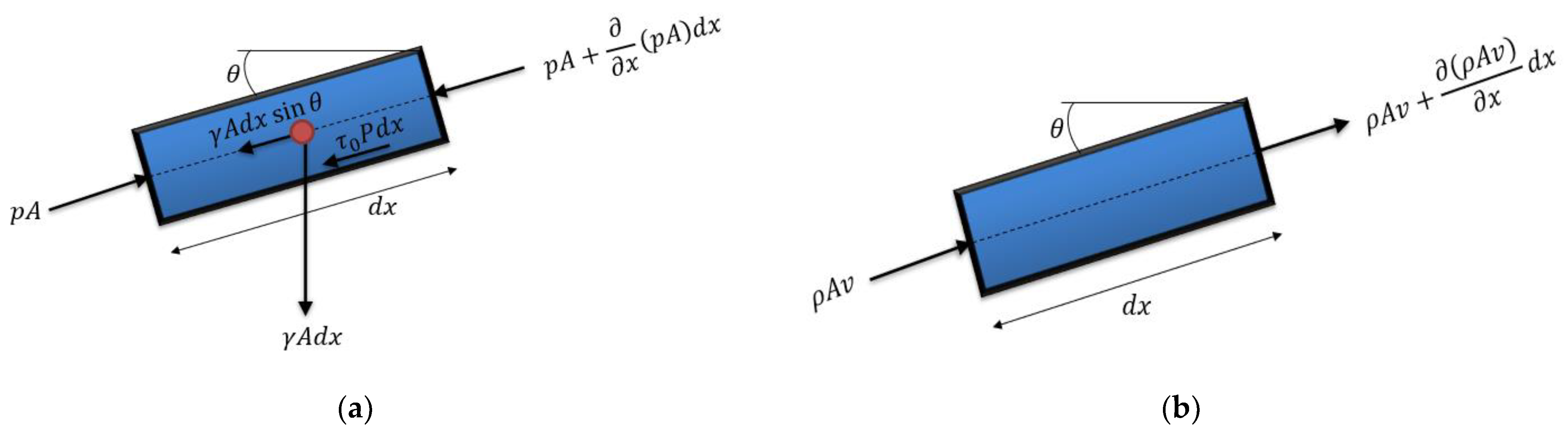
2.1. Water Hammer Modelling

Water hammer effects in pressurized pipelines are modeled based on momentum and continuity equations. Figure 1 shows the representative terms used to demonstrate these formulations. A free body diagram is presented in order to note the main variables for obtaining water hammer formulations. The used terms in Figure 1 are: $A$ = cross-sectoinal area, $p$ = pressure force, $\gamma$ = water unit weight, $x$ = distance in the main direction of a pipeline, ${\tau }_0$ = shear stress, $P_w$ = pipe perimeter, $\rho$ = water density, $\theta$ = pipe slope, and $v$ = water velocity.

The momentum equation is obtained considering Newton’s second law ($\sum F_x=m dv⁄dt)$, where $F_x$ represents forces in the main direction of a pressurized pipeline, $m$ is the water mass, and $\frac{dv}{dt}$ is the total derivate of water velocity over time. Considering all forces that are acting and replacing, then:

$$\frac{\partial v}{\partial t}+g\frac{\partial H}{\partial x}+\frac{fv\left|v\right|}{2D}=0$$

(1)

where $\frac{\partial v}{\partial t}$ = local water velocity term, $g$ = gravitional acceleration, $\frac{\partial H}{\partial x}$ = partial derivate of hydraulic grade line with regard to the main direction of a pipeline, $f$ = friction factor, and $D$ = internal pipe diameter.

The continuity equation is formulated based on Figure 1b, obtaining the expression presented as follows:

$$\frac{\partial H}{\partial t}+v\frac{\partial H}{\partial x}+\frac{a^2}{g}\frac{\partial v}{\partial t}=0$$

(2)

where $\frac{\partial v}{\partial x}$ = water convective velocity, $a$ = wave celerity, $\frac{\partial H}{\partial t}$ = partial derivate of hydraulic grade line over time, $g$ = gravitational acceleration, and $\frac{\partial H}{\partial x}$ = partial derivate of hydraulic grade line over space.

There is no numerical resolution for the differential formulations system composed by Equations (1) and (2), so the Method of Characteristics (MOC) is applied as a numerical technique resolution. To apply the MOC, a single pipeline with a total length (L) is divided in N segments, then: $∆t=\frac{L}{N_t}$ and $∆t=\frac{∆x}{a}$. Figure 2 shows the used calculation grid for applying MOC. Utilizing the finite differences scheme, the characteristic lines $C^{+}$ and $C^{-}$ are determined with Equations (3) and (4):

$$C^{+}\{\frac{g}{a}\frac{\partial H}{\partial t}+\frac{\partial v}{\partial t}+\frac{fv\left|v\right|}{2D}=0 \frac{dx}{dt}=+a$$

(3)

$$C^{-}\{-\frac{g}{a}\frac{\partial H}{\partial t}+\frac{\partial v}{\partial t}+\frac{fv\left|v\right|}{2D}=0 \frac{dx}{dt}=-a$$

(4)

The positive and negative characteristics are expressed as follows:

$$Q_P=C_P-C_a{H}_P$$

(5)

$$Q_P=C_n+C_a{H}_P$$

(6)

where $C_a=\frac{gA}{a}$.

If $H$ and $v$ values are known in points A and B, then

$$C_P=Q_A\frac{gA}{a}{H}_A-\frac{f∆t}{a}{Q}_A\left|Q_A\right|=0$$

(7)

$$C_n=Q_B\frac{gA}{a}{H}_B-\frac{f∆t}{a}{Q}_B\left|Q_B\right|=0$$

(8)

Equations (5) and (6) are basic algebraic relationships that can be used to describe transient propagation of hydraulic grade line and water flow rate. Solving simultaneously Equations (5) and (6), then:

$$Q_P=0.5\left(C_P+C_n\right)$$

(9)

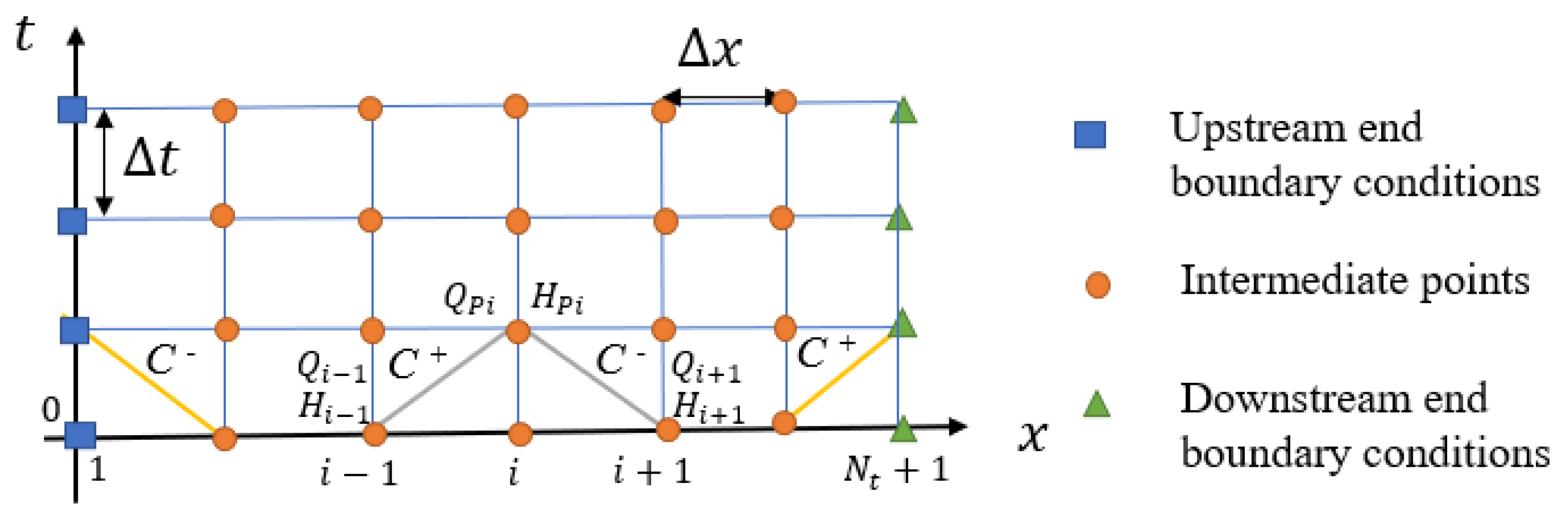
2.2. Boundary Conditions for MOC

At the ends of a pressurized pipeline, only one of the compatible equations is available in the two unknown variables $H$ and $Q$. For the upstream boundary, the characteristic curve $C^{-}$ is valid, while for the downstream boundary, the characteristic curve $C^{+}$ is valid. An additional equation is required in each case that specifies $Q_P$ or $H_P$, or some relationship between them. Figure 3 illustraes a grid scheme for computing intermediate points based on upstream and downstream boundary conditions. Additional equations for a constant-head reservoir, a pump, a regulating valve, and an air vessel are shown in

Table 1. Additional equations for calculating boundary conditions.

Element	Scheme	Considerations and Additional Equations	Equations System	Notation
Constant-head reservoir		The boundary condition for a constant-head reservoir is computed neglecting entrance head losses as: $H_P=H_{res}$	(10)	$H_{res}$ is the water level of a reservoir.
Pump		Based on pump characteristic curve for each time step as:$Q_P=\frac{2-B_{1}N{C}_a-\sqrt{{\left(B_{1}N{C}_a-2\right)}^2-4C_1{C}_a\left(A_1{C}_a{N}^2+C_P+C_n\right)}}{2C_1{C}_a}$	(11)	$A_1$, $B_1$, and $C_1$ are constants of a pump curve, and $N$ is the rotational speed.
Valve		The boundary condition in a regulating valve is obtained based on steady-state head loss equation as: $Q_P=\frac{-2+\sqrt{4+2\frac{K_V{C}_a}{g{A}^2}\left(C_P+C_n\right)}}{\frac{K_V{C}_a}{g{A}^2}}$	(12)	$K_V$ is the head loss coefficent obtained experiment20ally.
Air vessel		The equation of an air vessel is obtained considering the polytropic law $(H_{P,air}{V}_{P,air}^{p_c}=C)$, which needs to be solved simultaneously with the following five equations: $Q_{P,orifice}=\left(C_P-C_n\right)-\left(C_{a,i}+C_{a,i+1}\right)H_P$$Q_{P,orifice}=C{A}_o\sqrt{2g\Delta H_P}$$H_{P,air}=H_P+H_b-z_P-\Delta H_{P,orifice}$$V_{P,air}=V_{air}-A_C\left(z_P-z\right)$$z_P=z+0.5\left(Q_{P,orifice}+Q_{orifice}\right)\frac{\Delta t}{A_c}$	(13)	$H_{P,air}$ is the absolute pressure head at the end of an analysed time step, $V_{P,air}$ is the air volumne at the end of an analysed time step, $V_{air}$ is the air volume, $Q_{P,orifice}$ is the flow through the orifice,$A_o$ is the cross-section of the orifice, $C$ is the discharge coefficient of the orifice, $p_c$ is the polytropic coefficient (usually takes a value of 1.2), $z$ is the initial elevation of the free surface, $H_b$ is the barometric pressure, $C$ is the constant computed in the initial condition of the air vessel, $z_p$ is the free surface elevation at the end of the time step, and $A_c$ is the cross-section of the air vessel.

.

2.3. Turbine Modelling

The operational performance of a turbogenerator can be identified through a particular valve type equipped with modified characteristics that are associated with customized closure maneuvers. Although this approach may model the majority of system configurations and scenarios, it does not take into account the specific parameters of the turbine runner and guide-vane devices, nor does it address the overspeed of the turbine wheel and its intricate interaction with the conveyance system. The turbine as a hydraulic dynamic orifice resistive element has been simulated by [14,15,24], where the head lost by the flow rate is characterized by the formula of a hydrodynamic orifice equipped with variable discharge and rotational speed coefficients, as shown:

$$q_T=C_g{C}_s\sqrt{h_T}$$

(14)

where $q_T$ = relative flow through the turbine orifice, $h_T$ = relative turbine head available, $C_g$ = opening gate coefficient, and $C_s$ = the runner’s rotational speed coefficient.

The mathematical representation of turbomachinery parameters can be based on the specification of the relationship between flow rate $Q$, speed $N$, head $H$, and torque $T$, which are referred also to as pump characteristics. Some parameters can be defined as dimensionless values related to the point of best efficiency (also known as nominal or rated conditions) to be used as reference in different applications [6,23,25,26]:

$$q=\frac{Q}{Q_R}; h=\frac{H}{H_R}; n=\frac{N}{N_R}$$

(15)

$C_s$ is calculated using Equation (16).

$$C_s=1+\frac{{\alpha }_R-1}{{\beta }_R-1}\left(\frac{n}{\sqrt{h}}-1\right)$$

(16)

where ${\alpha }_R$ = relative runaway discharge (Q_RW/Q_R), ${\beta }_R$ = relative runaway rotating speed (N_RW/N_R), $n$ = relative runner speed, and $h$ = relative turbine net head.

The net hydraulic turbine torque ($T_H$) is another important parameter to characterize a turbine, which is related to the electromagnetic generator resistance torque ($T_G$) as follows:

$$T_H-T_G=I\frac{2\pi }{60}\frac{d\omega }{dt}$$

(17)

in which $I$ = rotaring mass inertia, and $\omega$ = angular speed.

The formulation for simulating the hydraulic rated torque actuating ($T_{H,R}$) is presented by Equation (18):

$$T_{H,R}=\frac{60}{2\pi }\frac{\gamma {\eta }_R{Q}_R{H}_R}{N_R}$$

(18)

where $\gamma$ = water unit weight, ${\eta }_R$ = unit rated efficiency, $Q_R$ = turbine rated discharge, $H_R$ = turbine rated head, and $N_R$ = turbine rated speed.

Assessing the efficiency is a complicated task that depends on numerous parameters. The following pair of equations can be used:

$$\{{\eta }_R\frac{N}{N_R} for N<N_R C_g\left(\frac{N_{RW}}{N_{RW}-N_R}-\frac{N}{N_{RW}-N_R}\right){\eta }_R for N>N_R$$

(19)

where $N$ = rotational turbine speed, and $N_{RW}$ = runaway rotational speed.

Equation (19) is based on turbine parameters, and it can be utilized as a dynamic boundary condition for assessing the extreme pressure occurrence in a hydropower system. However, Equation (14) comprises of two unknowns, so another condition must be established. Assuming that the losses at the junctions between the pipe and turbine are negligible, the transient net head can be approximated by $H=H_{P,i}-H_{P,i+1}$. Considering equations of MOC, then:

$$H=\frac{C_P-Q_P}{C_{a,i+1}}-\frac{Q_P-C_n}{C_{a,i}}$$

(20)

The Newton–Raphson method is used to obtain $Q_P$ as follows:

$$Q_{P,j}=Q_{P,j+1}-\frac{f\left(Q_{P,j-1}\right)}{f^{\prime }\left(Q_{P,j-1}\right)}$$

(21)

where $j$ = iteration number.

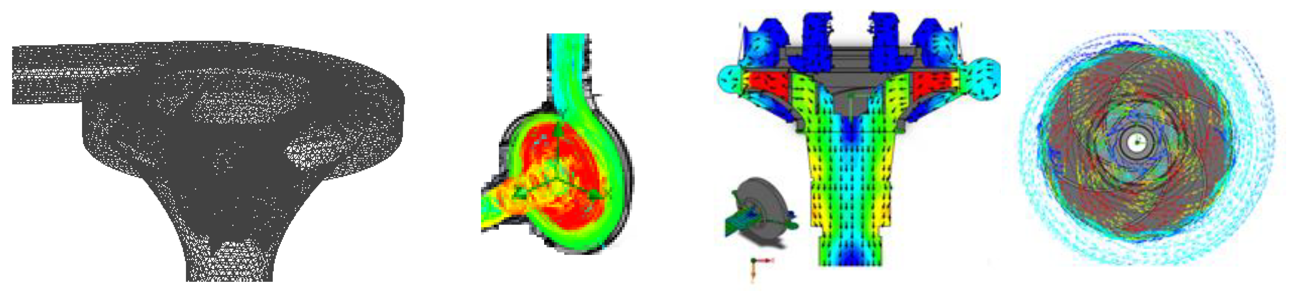
2.4. CFD Model Description and Mesh

The transient flow modelling of a reversible hydropower system can be conducted using the Navier–Stokes equations in combination with steady-state equations as well as semi-empirical models. The numerical resolution can be performed using packages such as ANSYS, OpenFOAM, Flow3D, and FloEFD, among others. The commercial package FloEFD is a fully CAD-embedded CFD that appropriately simulates laminar, transitional, and turbulent flows. Dynamic meshes can be considered for modelling rotating components of a reversible hydropower system based on a suitable coordinate system and angular velocity. The conservation and momentum equations in the conservation form are presented below [26,27,28,29,30]:

$$\frac{\partial \rho }{\partial t}+\frac{\partial }{\partial x_i}\left(\rho v_i\right)=0$$

(22)

$$\frac{\partial \rho v_i}{\partial t}+\frac{\partial }{\partial x_j}\left(\rho v_{i}v\right)+\frac{\partial p}{\partial x_i}=\frac{\partial }{\partial x_j}\left({\tau }_{ij}+{\tau }_{ij}^R\right)$$

(23)

where $v$ = water velocity, $\rho$ = water density, and ${\tau }_{ij}$ = viscous shear stress tensor. ${\tau }_{ij}$ is computed as (for water) [26]:

$${\tau }_{ij}=\mu \left(\frac{\partial v_i}{\partial x_j}+\frac{\partial v_j}{\partial x_i}-\frac{2}{3}{\delta }_{ij}\frac{\partial v_k}{\partial x_k}\right)$$

(24)

The Reynolds-stress tensor is based on Boussinesq assumption. ${\tau }_{ij}^R$ is computed as follows [26]:

$${\tau }_{ij}^R={\mu }_t\left(\frac{\partial v_i}{\partial x_j}+\frac{\partial v_j}{\partial x_i}-\frac{2}{3}{\delta }_{ij}\frac{\partial v_k}{\partial x_k}\right)-\frac{2}{3}\rho k{\delta }_{ij}$$

(25)

where $\mu$ = dynamic viscosity coefficient, ${\mu }_t$ = turbulent eddy viscosity coefficient, $k=$ turbulent kinetic energy, and ${\delta }_{ij}$ = Kronecker delta function.

The $k-\epsilon$ turbulence model has been extensively used for modelling transient flows, in wchich $\epsilon$ represents the turbulent dissipation [27]:

$${\mu }_t=f_u\frac{C_u\rho k^2}{\epsilon }$$

(26)

where $C_u$ is a constant and $f_u$ is a turbulent viscosity factor computed by:

$$f_u={\left(1-e^{-0.0165\frac{\rho \sqrt{k}y}{\mu }}\right)}^2\left(1+\frac{20.5\mu \epsilon }{\rho k^2}\right)$$

(27)

where $y$ is the distance from the wall.

Furthermore, 3D CFD simulations have been performed [26,27] to understand the behavior of all hydraulic variables and components during a transient flow modelling in a reversible hydropower system using the FloEFD package. The discretization of temporal derivatives was conducted with the finite volume method in combination with a second-order spatial scheme. A rectangular mesh was configured with an appropriate number of cells that can represent all hydraulic phenomena.

The pair composed for pressure and water velocity was calculated using the SIMPLE algorithm. Complete characteristics of the PATs and turbines were drawn using SolidWorks since it is suitable to represent 3D surfaces. The geometry of a pump working as a turbine or a classical turbine were completely represented considering elements such as volutes, impellers, draft tubes, and the outlet section [26,27]. The computational domain was established considering the solid/water interface, a suitable number of cells that can represent hydraulic devices, and an appropriate coordinate system.

To ensure the proper and acceptable accuracy of the results, the discretization mesh followed a typical Mesh Sensitivity Analysis (MSA), in which the density of cells is gradually increased and the solution is re-assessed towards an independence on the mesh size [28,29,30]. The discretization of the mesh was performed by assuming an initial coarse mesh with a total number of cells equal to 35,888, followed by a mesh refinement process. This process stopped when the difference in the head drop between consecutive meshes was less than 1%, which occurred for mesh with 135,472 cells (

Table 2. Mesh Sensitivity Analysis towards independence on the mesh size.

Mesh	Number of Fluid Mesh Cells	Number of Solid Mesh Cells	H	Error (%)	Duration
Mesh 1	35,888	25,378	9.8		0.15 h
Mesh 2	60,381	30,229	6.4	34%	0.49 h
Mesh 3	110,691	60,088	5.8	9%	2.23 h
Mesh 4	121,936	71,162	5.4	6%	2.52 h
Mesh 5	134,152	81,291	5.2	3%	3.28 h
Mesh 6	135,472	88,364	5.1	1%	3.33 h

). The mesh was refined around the pipe wall and in turbine blades, since important changes are expected and velocity fields are well represented in different turbine studies (Figure 4).

3. Dynamic Effects in Hydropower Systems

Dangerous runner lifting-up (RLU) accidents regarding propellers of Kaplan turbines in low-head hydropower stations were studied by using 3D computational fluid dynamics (CFD) to simulate the load rejection transients with guide-vane closing. It was found that by using any linear closing rule of the guide vane, the upward axial water force on the runner was larger than the weight of rotating parts that started before the guide vanes were closed, putting the hydropower station in a risky situation. It was the suction effect that caused the imbalance, induced by the high rotational speed runner that propels water downstream with a low discharge [31]. Another interesting study was developed by [32], showing a sensitivity analysis of the hydropower system parameters to the rotation speed and discharge. The pressure pulsation characteristics with different typical guide-vane closures were analyzed during the load-reduction process. In [33], stability problems in a hydropower station were analyzed using a nonlinear hydropower generation system for the load rejection transient process, where the authors carried out a dynamic safety assessment of the evolution behavior in the transient process. Thus, the framework of dynamic safety assessment aiming at transient processes should not only provide the guidance for safe operation, but also supply the design standard for hydropower stations.

Correctly, determining and mathematically characterizing the physical cause of the disturbance phenomena is essential, and the analysis strategy depends on the planning phase. Once the hydropower physical characteristics have been specified, various relevant scenarios must be chosen and assessed for transient pressure changes as precisely as possible during the planning stage. Water hammer analysis is crucial during the design process to identify the optimal solution that guarantees safety and minimizes risk as soon as possible. This should be accompanied by the creation of specific operating procedures to regulate transient pressure variations and other associated dynamic effects. Special protection devices may be considered if a benefit–cost ratio is presented. The primary objective is to avoid major damage to hydraulic installations and their associated components. Pressure surges can cause leaks or even a pipe rupture in water distribution systems, while sub-atmospheric conditions are usually associated with cavitation, water column separation, and severe transient events that can provoke in-pipe buckling phenomena [16].

In the hydraulic modelling of hydropower plants, the maneuvers that shall be considered are as follows: (i) start-up operation; (ii) stoppage of a turbomachine with a controlled closure of a shutter (i.e., guide vane); (iii) load rejection without the actuation of a shutter; and (iv) load rejection with the simultaneous actuation of a shutter, which is typically the most unfavorable when it is combined with high points of the hydraulic circuit with variations in the water level at the intake and outlet.

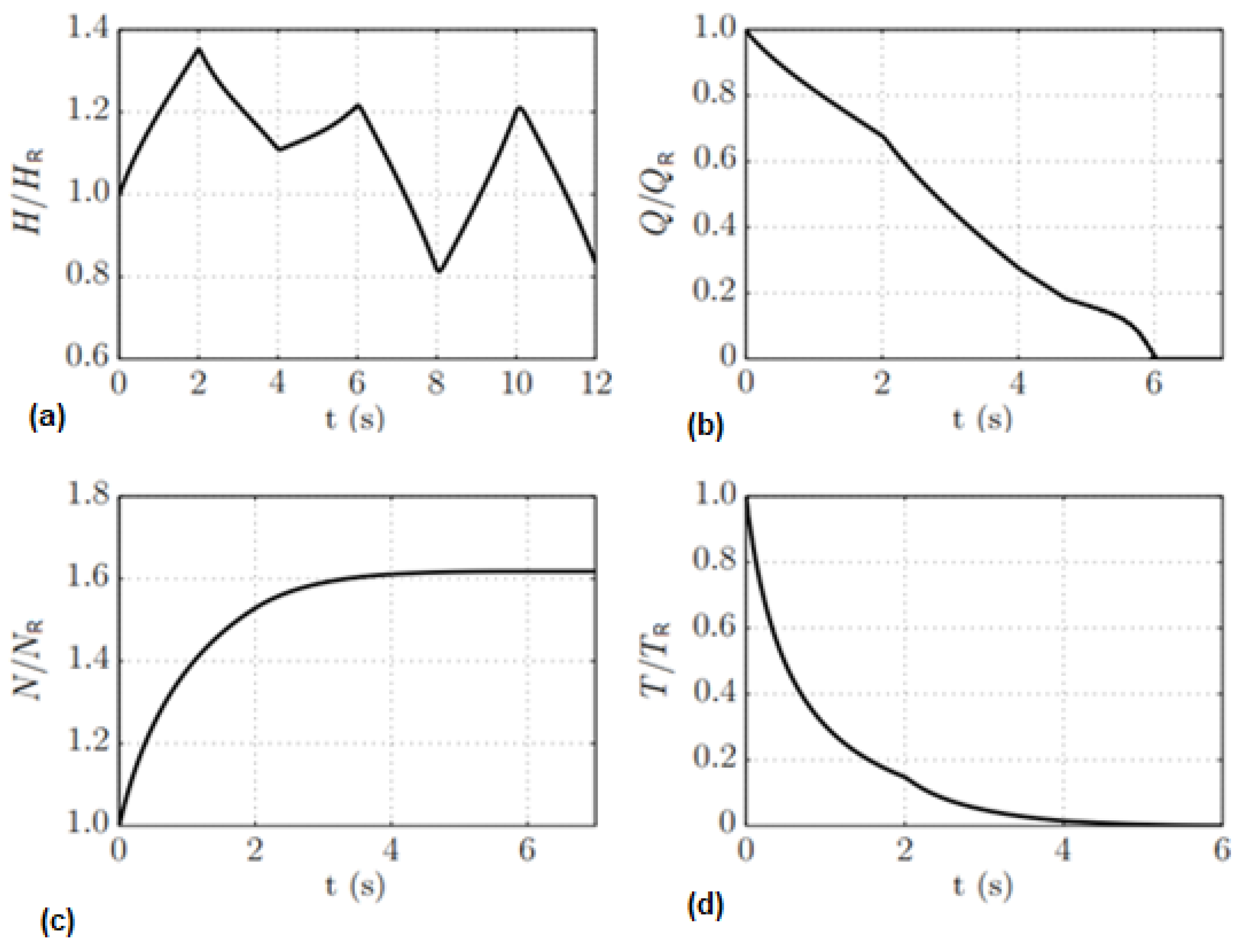
3.1. Overspeed Effect Due to Full-Load Rejection

When planning long conveyance systems associated with hydropower plants, it is essential to consider the overspeed effect. Depending on the characteristics of the hydromechanical equipment, sudden increases in rotational speed can cause significant discharge fluctuations that result in relevant absolute pressure head pulses. Over extended period conditions for a grid-connected system, the turbine speed is approximately synchronized with the frequency of the high-capacity electrical grid. This maintains a constant speed, which is achieved by balancing the magnetic torque generated by the generator and the hydraulic torque. At full-load rejection, the runner speed increases rapidly until it reaches its maximum value. Impulse turbines typically feature a deflector that rapidly redirects the flow away from the runner. The discharge can be controlled by a slower regulated closure maneuver, which allows rapid responses with regard to the wheel runaway. The combination of pressure and overspeed control in hydropower systems equipped with reaction turbines is riskier. Francis turbines have different behaviors depending on the characteristics of the specified speeds ($n_s$), as follows: (i) for low values, the water flow decreases with transient overspeed, while the guide vane remains at a constant overture; and (ii) for high values, an increasing trend is presented for the water flow [15,24].

The affinity laws for turbomachines are expressed by Equation (28), which represents the mathematical relationship between the rotational speed ($N$), flow rate ($Q$), head ($H$) and pump power ($P$). The specific speed is then given by Equation (29).

$$\frac{n_1}{n_2}=\frac{Q_1}{Q_2}=\sqrt{\frac{H_1}{H_2}}=\sqrt[3]{\frac{P_1}{P_2}}$$

(28)

in which results $n_s$ (rpm), which can be expressed based on (m, m³/s) or on (m, kW) as follows:

$$n_s=n\frac{Q^{1/2}}{H^{3/4}} or n_s=n\frac{P^{1/2}}{H^{5/4}}$$

(29)

To evaluate the overspeed effect in a turbogenerator, the relative overpressure values shown in Figure 5 as a function of the specific turbine speed $n_s$ and the relations $Tw/Tm$ and $T_c/TE$ are estimated.

The start-up time of rotating masses, T_m (s), is defined based on Equation (22):

$$T_m={10}^{-3}\frac{W{D}^2}{3575}\frac{{n_R}^2}{P_R}$$

(30)

where $n_R$ (rpm) is the nominal runner speed, $P_R$ the reference power (kW) and $W{D}^2=4gI$ (N·m²).

T_W is the hydraulic inertia time constant, defined by the following equation:

$$T_w=\frac{L}{gS}\frac{Q_R}{H_R}$$

(31)

where $L$ = pipe length (m); $Q_R/S$ = initial steady flow velocity (m/s); $H_R$ = net head under rated conditions (m).

Tc and TE are wicket gate closure time maneuver and elastic time, respectively.

To apply Figure 5 using a calibrated model, a first estimation of the specific speed, $n_s$, is required, which depends on the turbine runner shape. Let us consider the case for $n_s$ = 250 rpm (m, kW), which corresponds to a runner of ${\alpha }_R$ (relative runaway discharge) around 0.9, characterized by a diagonal entrance flow into the impeller. If the ratio of closure time and elastic time ($TE=2L/a$) is around 12.5 and the ratio of hydraulic inertia time ($T_w$) and the start-up time ($T_m$) is less than one, the relative upsurge should be expected to be around only 10% (please follow green arrows from 1 to 3). However, a smaller $n_s$ (around 165 rpm (m, kW)) corresponds to ${\alpha }_R$ = 0.65, which means a flow reduction of around 35% can induce an overpressure between 20 and 35% depending on the pipe length, the inertia of the rotating mass and the closure time (follow blue arrows from 1 to 3). The influence of the runner shape, inertia, pipe length and time of flow reduction are critical parameters in hydropower operating analysis.

A thorough examination of the runaway effect was conducted on a standard hydropower system where the closure of the flow control shutter (for instance, guide vane) or the implementation of any protection device is not acting. Thus, the system is isolated in order to study the water hammer phenomenon induced by the runaway conditions. Several simulations were performed while varying mass inertia ($I$) and specific speed ($n_s$). Figure 6 displays the maximum relative absolute pressure head at the upstream part of the turbine for different combinations of a set of pairs composed by $I$ and $n_s$ [34,35].

A decreasing trend in the water flow resulting from low specific-speed turbines operating in runaway conditions with small inertia turbines, associated with small sizes, generates an important overpressure with propagation along the all-conveyance system. On the other hand, turbines fitted with higher specific-speed runners exhibit the opposite effect. The time taken by the runner to achieve its runaway speed is influenced by the inertia of the rotating masses, consequently varying the flow through the turbine. As a result, the lower the mass inertia magnitude, the more substantial the transient regime associated upsurges.

The analysis shows that a turbine with a low specific-speed and small rotating mass inertia produces particularly high values of absolute pressure during the transient runaway critical condition, which could reach an overpressure of approximately 40% over the rated conditions. This may induce extreme pressures along the all-hydraulic conveyance system and jeopardize the hydropower controls and operation.

The gradual closing of the throttle valve in the downstream section of a long penstock and the simultaneous acceleration of the turbine runner result in unsteady flow condition, which can be responsible for strong pressure fluctuations. The following simulation is based on a typical hydropower plant with a turbine with a specific speed of ns = 100 rpm (m; kW), and a penstock with a total length of 4000 m. The variation of the main parameters is shown in Figure 7.

The initial condition for the simulation is the steady state in which the turbomachine operates at constant head and flow. At the time t = 0 s, the full-load rejection occurs and the guide vane is automatically actuated. Since the turbine has a low n_s value, the runaway causes a considerable reduction in flow with a high upsurge, even greater than that caused by the closing of the guide vane, resulting in the first peak in head, visible in Figure 7a at about t = 2 s. At this point, the discharge reduction is no longer as strongly influenced by the overspeed effect and begins to be controlled mainly by the flow control (Figure 7b).

As the impeller continues to accelerate, the turbine deviates significantly from its rated conditions and reduces the drive torque due to the outflow reduction until an equilibrium is reached when the speed tends to stabilize (Figure 7c,d). In the first few seconds, now without the resistive effect of the magnetic torque applied by the electric machine (generator), the rotor rapidly increases its speed in the first two seconds, as shown in Figure 7c. The second peak pressure value visible in Figure 7a corresponds to the complete closure of the guide vane at t = 6 s. The chosen example represents a particularly unfavorable system, where the overspeed effect causes more damage than the closing of the flow control valve itself, due to the large inertia versus a small machine inertia. Amongst the various emergency operations that a hydropower system may encounter during its operational lifespan, the most severe could possibly be a full-load rejection followed by the activation of a discharge shutter. To mitigate this situation, typical systems have sensors that detect a full-load rejection occurrence and actuate the guide vane to reduce water volume rate and control the rotational speed of the runner.

With the necessary computational tools, it is easy and interesting to study the complex interactions that occur during full-load rejection by performing sensitivity analyses with respect to the characteristic parameters and the different operating conditions.

3.2. Influence of Other Characteristic Parameters

The same turbomachine used in the case study shown in Figure 7 was then used to investigate the influence of the length L on the penstock and its interaction with the closing time $t_C$ of the guide vanes (Figure 8). Sensitivity analysis was developed in this section, and it relates to the full-load rejection scenario with the consequent closure of the turbine guide vane. Figure 8 shows the maximum relative upsurge for different pipe lengths ($L$), between 1000 and 4000 m, to show how small hydropower solutions usually with long penstocks can be quite dangerous due to the water column influence in the water hammer event.

Such an analysis allows us to also illustrate the dependence of the transient overpressure on the turbine guide-vane closure time $t_C$, the pipe length $L$, and the wave speed propagation of the pressure waves associated with different types of pipe materials.

On closer inspection, it becomes clear that the classification of a closure maneuver as fast ($t_C$ $\le$ $T_E$) or slow ($t_C$ > $T_E$) as a relative concept depends on the elastic wave speed associated with the material properties of the pipes. For a given water system, the transient overpressure caused by a slow maneuver depends essentially on the average fluid velocity (and consequently on the discharge) and on the closing time of the flow control device. The maximum value can be estimated based on the Michaud formula for a typical slow closing maneuver. Unlike a fast maneuver, the maximum overpressure in this case is independent of the wave speed. Figure 9 shows that each curve for $t_C$ > $T_E$ = $2L/a$ remains approximately constant, regardless of the value of $a$.

In Figure 8, for fast maneuvers, i.e., maneuvers with $t_C$ < $TE$, the transient overpressure surpasses 50% of the rated pressure. In fact, for fast maneuvers, the transient overpressure depends only on the wave speed and the initial pipeline flow velocity during steady-state conditions. As can be seen observed in Figure 9, for $t_C$ values larger than $TE$, the lower the value of $t_C$, the larger the transient overpressure. The slope of the curves is mild for relatively large values of $t_C$. The slopes of such curves, however, become steep as $t_C$ approaches $T_E$. For tc values higher than $T_E$, the value of the transient overpressure becomes invariable.

Hence, the most dangerous cases are those with large values of wave speed and $a$ and small values of tc. For the case with $a$ = 1400 m/s and $t_C$ = 6 s, the transient overpressure surpasses almost 70% of the rated pressure. For the case with $a$ = 1400 m/s and a slightly longer valve maneuver, namely $t_C$ = 8 s, the transient overpressure surpasses about 45% of the rated pressure and can be estimated by the Joukowsky formula. For slow maneuvers, i.e., for $t_C$ values beyond $TE$, the transient overpressure can be estimated by the Michaud’s formula. For a given tc value, transient overpressure increases with increments until $t_C=T_E$. For $t_C>T_E$, transient overpressure decreases with increments. For an optimal operation of pumped hydro storage-based energy systems, a compendium of current challenges and future perspectives can be found in [36].

4. Comparisons between Modelling and Laboratory Tests for Different Type of Turbines and Specific Speeds

Three experimental set-ups were used to obtain results from the models’ calibration: (i) Classical turbines of Francis and Kaplan (with fixed blades) or propeller [14,15,16,23,24]; and PATs (ii) radial and (iii) axial [21,28,29,30,34,35,37]. However, a brief description of them is provided (Figure 10).

-

For Francis and Kaplan with fixed blades (propeller)

An experimental facility (Figure 10a) was developed at LNEC (National Laboratory of Civil Engineering—Lisbon, Portugal), composed of upstream reservoirs with different water levels (R1 and R2), a gallery, a penstock and, downstream, the powerhouse (see Figure 1). The data acquisition system was installed in the powerhouse to obtain instantaneous values of turbine discharge, Q, runner speed, N, and piezometric head, upstream of the turbine, H1. The measurement equipment was connected to a computer and to the protection device action command. In the experimental facility, the total length of the hydraulic circuit was 110 m, with diameters of 0.200 m for the gallery and 0.125 m for the penstock. Along the conveyance system, there were some curves and some control valves. The spiral case of the turbine was adapted in order to be able to test three types of reaction turbine runners.

-

For radial PAT

The experimental installation (Figure 10b) consists of a hydraulic loop. The hydraulic circuit is composed of a pipe of high-density polyethylene (HDPE), with Dint = 0.043 m and a length of 100 m, which connects the pressurized vessel to the turbomachine. At the downstream end, the water is discharged into a free surface tank equipped with a triangular weir. The turbomachine is a horizontal, single-stage pump-as-turbine (PAT) KSB model Etanorm 32–125.

Experimental tests were carried out in the CERIS-Hydraulic Laboratory of Instituto Superior Técnico from the University of Lisbon for a radial and an axial reaction machine with small size. A small pressurized system was installed in order to develop the experimental test. The facility scheme is composed of:

-

For axial PAT

In this set-up (Figure 10c), the nominal diameter of the turbine model to transport the maximum available flow-rate in the installation (13.8 L/s) was hence designed for 85 mm. The hub houses the ceramic bearings and the main shaft of the turbine. The upstream bulb was elongated to obtain straighter velocity streamlines approaching the runner, which has the second advantage of providing a better reading in the pressure transducer. The runner and the bulb were produced separately in different materials: the runner in bronze, the bulb in black POM (polyoxymethylene). The thickness of the blade of 1.7 mm was chosen after an analysis of the structural resistance, corresponding to a safety factor of 3, considering a pressure of 30 m and the momentum for 1600 rpm.

4.1. PAT Radial Runners—Low ns

For a radial turbine runner tested in the laboratory, $n_s$ = 51 rpm (m, m³/s) for increasing rotational speed induced a typical wall effect, where the flow discharge reduced significantly. For example, for a constant head of 6 m and by varying the rotational speed between the rated conditions (i.e., $N$ = 1020 rpm) until we attained runaway conditions around the double of rated value, the flow reduced from 4.3 to 2.7 l/s, corresponding to a reduction of around 63%, which is very significant in terms of a water hammer event for a full-load rejection (Figure 11). As the rotational speed increases, the flow rate decreases and the head increases, induced by the centrifugal influence of a wall-type effect of cutting the flow discharge. This can be a dangerous event, inducing an upsurge peak that can be higher than the one induced by a valve or a guide-vane closure.

Figure 12 shows several operating points of the overspeed effect for the tested radial runner turbine under the runaway conditions, with an increase in $Q$ to 1.5 l/s from N = 600 to 2000 rpm against a 6.5 m head variation. This variation represents the induced problems of water hammer events in the pressure variation with the overspeed effect, considering the tested model scale. The rated conditions obtained in this tested radial turbine model scale corresponded to Q_R = 3.36 l/s; H_R = 4 m; N_R = 1020 rpm.

Under runaway conditions (with the increase in $N/N_R$) the flow reduces considerably, having an important role in the water hammer analysis (see Figure 13).

The flow reduces during overspeed conditions, with consequences for the water hammer events induced by PATs equipped with radial runners.

4.2. PAT Axial Runners—High n_s

However, for axial runners, the process happens the other way around. For example, an axial impeller was tested at $n_s$ = 283 rpm (m, m³/s) and it was found that at a constant head, e.g., $H$ = 2 m, the flow increases from 8 to 14 l/s with the increase of the rotational speed from 500 to 2750 rpm (Figure 14), because of the suction effect that occurs in these types of runners.

For axial turbines, the increasing of the flow induces a relief in pressure, as denoted in the tested axial turbine. It was verified that $Q$ increases to around 6 l/s when the rotational speed varies from N = 600 to 2000 rpm, against a quite insignificant small variation of 0.52 m in the head. So, the overspeed effect present under runaway conditions does not represent the induced problems of water hammer events in terms of overpressure with the overspeed effect, considering the tested model scale. The rated conditions obtained in this tested axial turbine model scale corresponded to Q_R = 4.4 l/s; H_R = 0.34 m; N_R = 750 rpm (Figure 15).

Under runaway conditions (Figure 16) (with the increase of $\frac{N}{N_R}$), the flow increases considerably, having an important role in avoiding upsurge. Hence, the overspeed effects do not represent a dangerous condition in axial turbines.

4.3. Francis Turbine—Low $n_s$

The dynamic behavior of a complete hydropower system was analyzed, composed by a long hydraulic circuit and different Francis turbines. The facility was designed to test different types of runners (from a low to a higher specific runner speed), through changing the turbine runners and adjusting water levels to new operating conditions. We established comparisons between the dynamic resistive orifice turbine model and experiments in a laboratory facility developed at LNEC/IST, for a full-load rejection of a radial turbomachine with ns = 130 rpm (kW, m). Upstream turbine head variation, rotational speed and flow discharge present a good fit between model simulation and experiments. The influence of the runaway conditions in the upstream head, flow variation and rotational speed are visible in Figure 17a, with particular evidence of velocity fields and pressure contours in the 2D simulation of the flow in the volute and crossing the prefixed guide vane (Figure 17b). When the runaway is attained, the wall effect in this low specific Francis turbine is noticed, inducing an upsurge peak.

The combination of two effects, such as runaway and guide-vane closure, is quite important in Figure 18. It shows a first overpressure peak (the maximum one) induced by overspeed conditions, when the runaway is quickly attained, in particular with turbines with small inertia and low specific speed; this is followed by a second overpressure peak that happens when the guide vane closes completely, corresponding to a complete full-load rejection.

4.4. Kaplan Turbine—High $n_s$

For axial turbine types (e.g., propeller or Kaplan turbines, with high specific ($n_s$) runner speed), the flow increases under runaway conditions ($Q_{RW}/Q_R={\alpha }_R>1)$.

Therefore, these phenomena are of great importance for the design of the penstock and its supports and anchors. Hence, the closing maneuver of the guide vanes does not seem to be the most dangerous effect. It is easy to act on the duration of complete closure to control it and avoid excessive increase beyond the maximum design pressure of the hydraulic circuit and power plant equipment. In this way, the runaway condition is achieved, and the suction effect induced by these types of runners (opposite to the Francis turbine’s low $n_s$ values, which induces a wall flow cut effect) induces flow, increasing and reducing the pressure head, as shown in Figure 19.

As analyzed for the Francis turbine, in this case of a Kaplan, for the combination of runaway and guide-vane closure events, the first peak of overpressure disappeared under runaway conditions and is only visible the upsurge due to the actuation of the guide-vane closure in a complete full-load rejection (in Figure 20).

The developed analyses based on mathematical modelling of 1D, 2D and 3D and specific experimental set-ups (for PATs and classical turbines—Francis and Kaplan) allowed us to enhance the characteristic parameter interaction during the main hydropower station operating maneuvers, to better understand the induced effects, possible pressure and flow oscillations, and extreme conditions associated with accidental or emergency situations and move towards a better sustainable and safe system.

5. Conclusions

The current paper explores the issue of unsteady pipe flows in reversible hydropower-pumping lines. The focus is essentially on turbine mode, although different boundary elements are mathematically formulated and exposed for a complete understanding of the system complexity. The numerical approaches presented, namely the method of characteristics formulation (MOC–1D) for long pipes, the dynamic orifice technique model for the behavior of a reaction turbomachine in turbine mode, and the CFD model (2D and 3D) for velocity fields and pressure contours were consubstantiated by experimental tests using different set-ups with long conveyance systems, as they induce the worst water hammer effects and are used in micro and small hydropower systems. Two experimental set-ups were used, composed by pumps as turbines (at IST laboratory) and reaction classical turbines (at LNEC laboratory). These mathematical models together with experiments allow for the estimation of extreme transient pressures, the rotational speed and flow discharge variation induced by the overspeed effect, followed by a full-load rejection scenario with the simultaneous closure of the turbine’s valve or guide vane.

An advantage of the numerical model when translating the turbine behavior based on a dynamic orifice technique is built on the characteristic parameters of the turbine that are known or can be estimated. The numerical approach presented in this research can be used in the design project stage to evaluate the system’s susceptibility to dangerous water hammer extreme pressures. In some cases, the runaway conditions can induce an overspeed of 2–2.5 N_R and an overpressure of up to 65% H_R, with significant interaction with the penstock fluid propagation along the all-hydraulic circuit.

The paper also presents sensitivity analyses, based on systematic numerical simulations, of typical water hammer scenarios involving PATs (radial and axial types), turbines (Francis and Kaplan types) and comparisons with experiments. These evaluations show the dynamic effects associated with reversible hydropower solutions when working in turbine mode because although it is less known in the expert literature, they can occur in micro, small and large pumped storage hydropower energy systems. Hence, it is found that the full-load rejection scenario can be dangerous for turbomachines with low n_s values, both with or without the closure of the turbine’s valve/guide vane. For low specific-speed and small inertia turbines, particularly used in micro or small hydropower plants, the transient overpressure can become significant by the overspeed effect that induces a type of wall effect, cutting the flow in few seconds and thus originating substantial upsurges that propagate along the hydraulic circuit. Conversely, in turbomachines with high n_s values, the overspeed effect can induce an increase in the flow discharge as a suction effect with a pressure drop, which is not dangerous for the hydropower system.

In fact, for low specific-speed turbines, as the turbine attains its runaway speed, the flow discharge through the turbine decreases, with such a reduction resulting in an overpressure sometimes larger than the one associated with the closure of the turbine’s valve/guide vane. The guide-vane closure time can be chosen in a controlled way, in order to not create dangerous effects for the system. It is worth mentioning that the water hammer issues are much more significant in long penstocks due to the water column inertia time that will influence the upsurge values when associated with fast closure maneuvers. Due to the characteristics of the valve/guide-vane maneuver, the effective closure can also be different to the total closure time, with the only real flow reduction happening near the closure time, which can transform a slow into a fast maneuver, with disastrous water hammer consequences that can put the power station or even the all-hydropower system in danger.

References

1. Burek, P.; Satoh, Y.; Fischer, G.; Kahil, T.; Jimenez, L.; Scherzer, A.; Tramberend, S.; Wada, Y.; Eisner, S.; Flörke, M.; et al. Water Futures and Solution: Fast Track Initiative (Final Report); IIASA: Laxemburg, Austria, 2016. [Google Scholar]
2. Ferroukhi, R.; Nagpal, D.; Lopez-Peña, A.; Hodges, T.; Mohtar, R.H.; Daher, B.; Mohtar, S.; Keulertz, M. Renewable Energy in the Water, Energy and Food Nexus; International Renewable Energy Agency: Abu Dhabi, United Arab Emirates, 2015. [Google Scholar]
3. Simão, M.; Ramos, H.M. Hybrid Pumped Hydro Storage Energy Solutions towards Wind and PV Integration: Improvement on Flexibility, Reliability and Energy Costs. Water 2020, 12, 2457. [Google Scholar] [CrossRef]
4. Rogner, M.; Troja, N. The World’s Water Battery: Pumped Hydropower Storage and the Clean Energy Transition; International Hydropower Association: London, UK, 2018. [Google Scholar]
5. Ramos, H.M.; Amaral, M.P.; Covas, D.I.C. Pumped-Storage Solution towards Energy Efficiency and Sustainability: Portugal Contribution and Real Case Studies. J. Water Resour. Prot. 2014, 6, 1099–1111. [Google Scholar] [CrossRef]
6. Carravetta, A.; Houreh, S.D.; Ramos, H.M. Pumps as Turbines: Fundamentals and Applications; Springer International Publishing AG: Cham, Switzerland, 2018; ISBN 978-3-319-67506-0. [Google Scholar] [CrossRef]
7. Kougias, I.; Patsialis, T.; Zafirakou, A.; Theodossiou, N. Exploring the potential of energy recovery using micro hydropower systems in water supply systems. Water Util. J. 2014, 7, 25–33. [Google Scholar]
8. Pérez-Sánchez, M.; Sánchez-Romero, F.J.; Ramos, H.M.; López-Jiménez, P.A. Energy Recovery in Existing Water Networks: Towards Greater Sustainability. Water 2017, 9, 97. [Google Scholar] [CrossRef]
9. Carravetta, A.; Del~Giudice, G.; Fecarotta, O.; Gallagher, J.; Morani, M.C.; Ramos, H.M. Potential Energy, Economic, and Environmental Impacts of Hydro Power Pressure Reduction on the Water-Energy-Food Nexus. J. Water Resour. Plan. Manag. 2022, 148, 04022012. [Google Scholar] [CrossRef]
10. Fontanella, S.; Fecarotta, O.; Molino, B.; Cozzolino, L.; Della Morte, R. A Performance Prediction Model for Pumps as Turbines (PATs). Water 2020, 12, 1175. [Google Scholar] [CrossRef]
11. De Marchis, M.; Milici, B.; Volpe, R.; Messineo, A. Energy Saving in Water Distribution Network through Pump as Turbine Generators: Economic and Environmental Analysis. Energies 2016, 9, 877. [Google Scholar] [CrossRef]
12. Lima, G.M.; Luvizotto, E., Jr.; Brentan, B.M. Selection and location of Pumps as Turbines substituting pressure-reducing valves. Renew. Energy 2017, 109, 392–405. [Google Scholar] [CrossRef]
13. Pérez-Sánchez, M.; Sánchez-Romero, F.J.; Ramos, H.M.; López-Jiménez, P.A. Improved Planning of Energy Recovery in Water Systems Using a New Analytic Approach to PAT Performance Curves. Water 2020, 12, 468. [Google Scholar] [CrossRef]
14. Ramos, H.; Almeida, A.B. Dynamic orifice model on waterhammer analysis of high or medium heads of small hydropower schemes. J. Hydraul. Res. 2001, 39, 429–436. [Google Scholar] [CrossRef]
15. Ramos, H.; Almeida, A.B. Parametric analysis of waterhammer effects in small hydropower schemes. J. Hydraul. Eng. 2002, 128, 689–697. [Google Scholar] [CrossRef]
16. Ramos, H.M.; Almeida, A.B.; Portela, M.M.; Almeida, H.P. Guidelines for Design of Small Hydropower Plants; Western Regional Energy Agency & Network: Enniskillen, Northern Ireland; Department of Economic Development: Belfast, Northern Ireland, 2000. [Google Scholar]
17. Pothof, I.; Karney, B. Guidelines for transient analysis in water transmission and distribution systems. In Water Supply System Analysis—Selected Topics; Ostfeld, A., Ed.; InTech: Rijeka, Croatia, 2012; pp. 1–21. [Google Scholar]
18. Boulos, P.; Karney, B.; Wood, D.; Lingireddy, S. Hydraulic transient guidelines for protecting water distribution systems. J. Am. Water Work. Assoc. 2005, 97, 111–124. [Google Scholar] [CrossRef]
19. Wylie, E.B.; Streeter, V.L. Fluid Transients; FEB Press: Ann Arbor, MI, USA, 1983. [Google Scholar]
20. Chaudhry, M.H. Applied Hydraulic Transients, 3rd ed.; Springer: New York, NY, USA, 2014. [Google Scholar]
21. Pérez-Sánchez, M.; López-Jiménez, P.A.; Ramos, H.M. PATs Operating in Water Networks under Unsteady Flow Conditions: Control Valve Manoeuvre and Overspeed Effect. Water 2018, 10, 529. [Google Scholar] [CrossRef]
22. Lima, G.M.; Luvizotto, E., Jr. Method to Estimate Complete Curves of Hydraulic Pumps through the Polymorphism of Existing Curves. J. Hydraul. Eng. 2017, 143, 04017017. [Google Scholar] [CrossRef]
23. Ramos, H.; Almeida, A.B. Experimental and Computational Analysis of Hydraulic Transients Induced by Small Reaction Turbomachines; APRH, LNEC.: Lisboa, Portugal, 2001. (In Portuguese) [Google Scholar]
24. Ramos, H.M. Simulation and Control of Hydrotransients at Small Hydroelectric Power Plants. Ph.D. Thesis, Technical University of Lisbon, Lisbon, Portugal, 1995. (In Portuguese). [Google Scholar]
25. Ramos, H.; Borga, A. Pumps as turbines: An unconventional solution to energy production. Urban Water 1999, 1, 261–263. [Google Scholar] [CrossRef]
26. Hanna, K.; Parry, J. Back to the Future: Trends in Commercial CFD. In Proceedings of the NAFEMS World Congress 2011, Boston, MA, USA, 23–26 May 2011. [Google Scholar]
27. Solid Works 2011. Flow Simulation. Available online: https://www.gsc-3d.com/training-solutions/ (accessed on 12 November 2022).
28. Simão, M.; Pérez-Sánchez, M.; Carravetta, A.; López-Jiménez, P.; Ramos, H.M. Velocities in a Centrifugal PAT Operation: Experiments and CFD Analyses. Fluids 2018, 3, 3. [Google Scholar] [CrossRef]
29. Simão, M.; Pérez-Sánchez, M.; Carravetta, A.; Ramos, H.M. Flow Conditions for PATs Operating in Parallel: Experimental and Numerical Analyses. Energies 2019, 12, 901. [Google Scholar] [CrossRef]
30. Simão, M.; López-Jiménez, P.A.; Ramos, H.M. CFD Analyses and Experiments in a PAT Modeling: Pressure Variation and System Efficiency. Fluids 2017, 2, 51. [Google Scholar] [CrossRef]
31. Liu, K.; Yang, F.; Yang, Z.; Zhu, Y.; Cheng, Y. Runner Lifting-Up during Load Rejection Transients of a Kaplan Turbine: Flow Mechanism and Solution. Energies 2019, 12, 4781. [Google Scholar] [CrossRef]
32. Zhang, M.; Feng, J.; Zhao, Z.; Zhang, W.; Zhang, J.; Xu, B. A 1D-3D Coupling Model to Evaluate Hydropower Generation System Stability. Energies 2022, 15, 7089. [Google Scholar] [CrossRef]
33. Li, S.; Yang, Y.; Xia, Q. Dynamic Safety Assessment in Nonlinear Hydropower Generation Systems. Complexity 2018, 2018, 1–8. [Google Scholar] [CrossRef]
34. Morgado, P.A.L. Mathematical Modelling to Simulate Dynamic Effects in Reversible Hydro Systems. Master’s Thesis, Instituto Superior Técnico, Universidade Técnica de Lisboa, Lisboa, Portugal, 2010. [Google Scholar]
35. Morgado, P.A.; Ramos, H.M. Pump as turbine: Dynamic effects in small hydro. In Proceedings of the World Renewable Energy Congress, Linkoping, Sweden, 8–13 May 2011; Hydropower Applications: Linkoping, Sweden, 2011. [Google Scholar]
36. Mahfoud, R.J.; Alkayem, N.F.; Zhang, Y.; Zheng, Y.; Sun, Y.; Alhelou, H.H. Optimal operation of pumped hydro storage-based energy systems: A compendium of current challenges and future perspectives. Renew. Sustain. Energy Rev. 2023, 178, 113267. [Google Scholar] [CrossRef]
37. Samora, I.; Hasmatuchi, V.; Münch-Alligné, C.; Franca, M.J.; Schleiss, A.J.; Ramos, H.M. Experimental characterization of a five blades tubular propeller turbine for pipe inline installation. Renew. Energy 2016, 95, 356–366. [Google Scholar] [CrossRef]
Figure 1. Freebody diagram applied to: (a) momentum equation; and (b) continuity equation.
Water 15 02034 g001
Figure 2. Calculation grid for MOC.
Water 15 02034 g002
Figure 3. Boundary conditions for MOC.
Water 15 02034 g003
Figure 4. Mesh definition and an example of velocity fields for 3D and 2D performed simulations.
Water 15 02034 g004
Figure 5. Relative overpressure induced by the turbine overspeed.
Water 15 02034 g005
Figure 6. Relationship between maximum relative overpressure head, inertia of the runner, and specific speed: (a) plan view and (b) 3D view, better showing the curvature significance effect for both inertia and specific-speed variation.
Water 15 02034 g006
Figure 7. Full-load rejection for a hydropower case study: (a) Relative pressure head; (b) Relative discharge; (c) Relative rotational speed and (d) Relative torque.
Water 15 02034 g007
Figure 8. Maximum relative overpressure for different combinations of hydraulic circuit length and flow control device closure time.
Water 15 02034 g008
Figure 9. Maximum relative upsurges for a typical hydropower with different characteristics: (a) 2D representation for wave speed, a , and guidevane closure time, t C , variation; and (b) 3D dependency on different combinations of these parameters.
Water 15 02034 g009
Figure 10. Three experimental set-ups for tests performed and calibration of developed mathematical models: (a) for classical turbines – Francis and Kaplan with fixed blades, (b) for the radial PAT, (c) for axial PAT.
Water 15 02034 g010
Figure 11. Different operating conditions for a radial runner by increasing rotational speed until to attain the runaway: (a) characteristic curves H-Q for different N; (b) pressure values and velocity fields for N = 810 and 1500 rpm.
Water 15 02034 g011aWater 15 02034 g011b
Figure 12. Operating points H-Q-N under runaway conditions in a radial runner.
Water 15 02034 g012
Figure 13. The influence of rotational speed on the fast variation of flow (Q/QR—color variation) for constant head values in a radial runner type.
Water 15 02034 g013
Figure 14. Different operating conditions for an axial runner by increasing rotational speed until to attain the runaway: (a) characteristic curves H-Q for different N; (b) stream lines and velocity fields (top), pressure contours values and shear stress (bottom) for N = 750 and 1500 rpm.
Water 15 02034 g014aWater 15 02034 g014b
Figure 15. Operating points H-Q-N under runaway conditions in an axial runner.
Water 15 02034 g015
Figure 16. The influence of rotational speed on the fast variation of flow (Q/QR—color variation) for certain constant head values in an axial runner type.
Water 15 02034 g016
Figure 17. Runaway effect in a Francis turbine with ns = 130 rpm (m, kW): (a) upstream head, flow and rotational speed variation, (b) flow velocity fields and pressure contours variation in 2D simulation for rated and runaway conditions.
Water 15 02034 g017
Figure 18. Francis turbine behavior (with low n s ) during a simultaneously runaway and guide-vane closure events.
Water 15 02034 g018
Figure 19. Runaway effect in a Kaplan turbine with n s = 400 rpm (m, kW): (a) upstream head, flow and rotational speed variation, (b) flow velocity fields and pressure contours variation in 2D simulation for rated and runaway conditions.
Water 15 02034 g019
Figure 20. Kaplan turbine behavior (with high n s ) during a simultaneously runaway and guide-vane closure events.
Water 15 02034 g020