Article

Prediction of Rainfall Time Series Using the Hybrid DWT-SVR-Prophet Model

1
College of Resource Environment and Tourism, Capital Normal University, Beijing 100048, China
2
State Key Laboratory of Urban and Regional Ecology, Research Center for Eco-Environmental Sciences, Chinese Academy of Sciences, Beijing 100085, China
3
State Key Joint Laboratory of Environment Simulation and Pollution Control, Research Center for Eco-Environmental Sciences, Chinese Academy of Sciences, Beijing 100085, China
4
University of Chinese Academy of Sciences, Beijing 100049, China
*
Author to whom correspondence should be addressed.
Water 2023, 15(10), 1935; https://doi.org/10.3390/w15101935
Submission received: 26 April 2023 / Revised: 15 May 2023 / Accepted: 17 May 2023 / Published: 20 May 2023
(This article belongs to the Section Hydrology)

Abstract

:
Accurate rainfall prediction remains a challenging problem because of the high volatility and complicated essence of atmospheric data. This study proposed a hybrid model (DSP) that combines the advantages of discrete wavelet transform (DWT), support vector regression (SVR), and Prophet to forecast rainfall data. First, the rainfall time series is decomposed into high-frequency and low-frequency subseries using discrete wavelet transform (DWT). The SVR and Prophet models are then used to predict high-frequency and low-frequency subsequences, respectively. Finally, the predicted rainfall is determined by summing the predicted values of each subsequence. A case study in China is conducted from 1 January 2014 to 30 June 2016. The results show that the DSP model provides excellent prediction, with RMSE, MAE, and R2 values of 6.17, 3.3, and 0.75, respectively. The DSP model yields higher prediction accuracy than the three baseline models considered, with the prediction accuracy ranking as follows: DSP > SSP > Prophet > SVR. In addition, the DSP model is quite stable and can achieve good results when applied to rainfall data from various climate types, with RMSEs ranging from 1.24 to 7.31, MAEs ranging from 0.52 to 6.14, and R2 values ranging from 0.62 to 0.75. The proposed model may provide a novel approach for rainfall forecasting and is readily adaptable to other time series predictions.

1. Introduction

Rainfall, as an essential process in the hydrological cycle, is one of the most studied components of hydrological and climate science, as it directly or indirectly affects our society [1]. Accurate rainfall prediction is vital in daily life, risk assessment, natural disaster prevention, and water resource planning and management [2,3]. However, the prediction of rainfall is a difficult task due to the dynamic complexity and nonstationary nature of measured hydrological data [4]. Models used for hydrometeorological time series prediction can be divided into physical process-driven models and data-driven models [5]. The former requires complex equations to be solved with large amounts of data, and it cannot be extended to new regions [6]. The latter learns long-term patterns of physical phenomena directly from data and can be quickly developed and easily implemented [7].
Statistical and machine learning methods are often used to develop data-driven models. Traditional statistical models, such as the autoregressive moving average (ARIMA) and multiple linear regression (MLR) models, may not be suitable methods [8], which only yield satisfactory results when predicting linear or near-linear time series and fail to capture nonlinear and nonstationary factors in hydrometeorological time series [9]. Machine learning techniques have a powerful learning capability ideal for modeling linear and nonlinear relationships in data without necessarily understanding the physical mechanisms associated with the data [10,11]. Therefore, various machine learning models have been applied for hydrometeorological time series prediction, such as the artificial neural network (ANN), support vector regression (SVR), Prophet, and random forest (RF) models. These models provide satisfactory predictions of nonlinear hydrological and meteorological processes [12,13,14,15].
Although these single methods have achieved breakthroughs in prediction performance, their shortcomings have also been exposed. For example, the SVR model has limitations in predicting highly nonstationary hydrological time series at different scales; moreover, prediction performance is influenced by the size of the data set and the parameters and kernel functions used [16]. The strong nonlinear mapping capability of neural networks has led to their increased application in climate data prediction. However, as the amount of data increases, the structure of neural networks becomes more complex, significantly decreasing the processing speed and leading to convergence to local minima, resulting in lower prediction accuracy [17].
In recent years, time series decomposition algorithms have been applied for feature extraction and prediction involving hydrometeorological time series. The combination of time series decomposition methods and machine learning has facilitated the development of hybrid models and improved prediction accuracy [18,19,20]. Apaydin et al. [21] used singular spectrum analysis to process monthly flow data and combined this approach with neural networks for prediction. The results showed that this method yields higher prediction accuracy than other single neural network models and can achieve more accurate river flow predictions. Ravansalar et al. [22] constructed a wavelet linear genetic programming (WLGP) approach to predict monthly flows at two stations. They compared the WLGP model with a linear genetic programming (LGP) model, a neural network model, a hybrid wavelet neural network model (WANN), and an MLR model. The results showed that the WLGP model could significantly improve the accuracy of flow predictions and other hydrological predictions. Samani et al. [23] predicted groundwater level (GWL) changes with a set of supervised machine learning (ML) models, i.e., ANN, adaptive neuro-fuzzy inference system (ANFIS), group method of data handling (GMDH), least square support vector machine (LSSVM), and the hybrid wavelet conjunction models. They found that the hybrid models perform better than single models, and the wavelet transform–least square support vector machine (WT-LSSVM) model obtained the best accuracy. However, the decomposed time series components usually exhibit different characteristics, and it is difficult for a single prediction method to accurately predict all components. Therefore, according to the characteristics of time series components, some scholars have used different models for prediction to further improve prediction performance [24,25]. Wei et al. [26] built a hybrid model (DWT-CLSTM-DCCNN) with discrete wavelet transform (DWT), long short-term memory (LSTM), and dilated causal convolutional neural network (DCCNN) to forecast monthly rainfall data. The results showed that the coupled model outperforms the benchmark models in prediction accuracy and peak rainfall capture. Khan et al. [27] combined the strengths of the Wavelet transformation (WT), ARIMA, and ANN to predict droughts. In the experiment, the combined model has improved accuracy compared to the single ANN and WT-ANN.
Among the many time series decomposition methods, seasonal decomposition and discrete wavelet decomposition have been widely used [28,29]. In the seasonal decomposition method, a time series is divided into the trend, periodic, and residual terms, which represent different typical characteristics, among which the predictability of the trend and periodic terms is generally high [30]. The residual term represents irregular fluctuations in time series with certain volatility and randomness, and thus, a machine learning model with excellent learning ability must be applied, otherwise it may lead to poor prediction performance in cases with detailed features. In contrast, in the DWT approach, specific frequencies are filtered at each scale, and the original data are decomposed into single-frequency components, thus smoothing the sequence and making it more conducive to model fitting and the prediction of each component [8]. The SVR model is based on the structural risk minimization criterion, which can capture the nonlinear features in data, is characterized by good generalization ability, and can improve prediction accuracy and speed [31], so it is suitable for high-frequency component forecasting. The Prophet model includes simple and intuitive parameters and yields a good prediction effect; notably, it can provide accurate predictions in cases with periodic data, many outliers, and large trend changes [32]. Thus, this model has advantages in the prediction of low-frequency components. Theoretically, the combination of DWT with SVR and the Prophet model can improve the accuracy of time series prediction, and the performance of this method deserves further exploration. No study has yet applied such a combined model for rainfall time series prediction.
This paper builds a hybrid model (DSP) with DWT, SVR, and Prophet to provide an accurate rainfall time series prediction. To this end, we first decompose the original data into high-frequency components and low-frequency components using DWT, and then, SVR is applied for high-frequency component prediction, and the Prophet model is used for low-frequency component prediction. Finally, the prediction results of each subseries are combined to obtain the final prediction results. The effectiveness of the DSP method is verified by using daily rainfall time series as a case study. Compared with the three baseline methods, the superiority of the DSP approach is verified. Moreover, the DSP model is used to predict rainfall from stations in different climate types to further verify its universality. Next, the seasonal decomposition method is compared with DWT to demonstrate the advantages of the proposed approach for data preprocessing. Overall, the DSP method decomposes complex rainfall time series into subseries with a single fluctuation frequency and establishes different models for different components, which improves the accuracy of rainfall time series prediction.
The rest of this paper is organized as follows. Section 2 presents the prediction method used in the DSP model, as well as the parameter optimization and model evaluation schemes. Detailed experimental results are given in Section 3. Section 4 discusses the applicability of the DSP model, the advantages of the DSP model in rainfall prediction, and improvements in the prediction accuracy compared to other models. Finally, a summary is presented in Section 5.

2. Methodology

2.1. Hybrid Model Based on DWT-SVR-Prophet

We propose a DSP model for rainfall time series prediction, and the framework is shown in Figure 1.
(i)
Data preparation and preprocessing: We construct a dataset with daily rainfall data from the National Meteorological Center. The validity and superiority of the model introduced in this paper are verified using this dataset. We preprocess the measured rainfall data to ensure the fitting effect of the applied machine learning model. This process is described in detail in Section 2.2.
(ii)
DWT processing: The rainfall time series are decomposed using DWT to obtain high-frequency subsequences with high randomness and volatility and low-frequency subsequences with high periodicity (see Section 2.3.1). This approach allows us to choose forecasting models based on the characteristics of each subseries.
(iii)
Hyperparameter optimization: The hyperparameters of the three methods in the coupled model are optimized to obtain the optimal prediction effect. Notably, the parameters of the DWT method are determined by referring to the previous literature, and a grid search method is used to set the hyperparameters of the SVR and Prophet models. The specific process of parameter selection is described in detail in Section 2.5.
(iv)
Rainfall prediction: The optimized SVR model and Prophet model are used to predict high-frequency subseries and low-frequency subseries, respectively. The prediction results for each subseries are summed to obtain the final prediction results.

2.2. Data Preprocessing

The data used in this paper were obtained from the National Weather Science Data Center (http://data.cma.cn, accessed on 25 April 2023). To construct the dataset, we selected daily rainfall data (from 1 January 2014 to 30 June 2016) from five stations in different climate zones. The rainfall statistics are shown in Table 1. It is worth mentioning that the annual average rainfall and rainfall frequency of station 59855, station 58345, and station 57348 are higher; the annual rainfall of station 54823 is moderate, and the precipitation frequency is the lowest; the annual average rainfall of station 56018 is the lowest, but the rainfall frequency is higher.
One of the prerequisites for a data-driven model is ensuring that the data quality meets the relevant modeling requirements [33]. Therefore, before performing data decomposition, the measured rainfall data need to be preprocessed, such as filling in missing values and normalizing the data. There were no missing values in the dataset used in this paper. To avoid the influence of extreme rainfall values and improve the accuracy of the machine learning algorithm, the maximum–minimum scaling method [34] was adopted to normalize daily rainfall data to between 0 and 1. The specific formula is as follows:
P n o r m = P i P min P max P min
where Pnorm, Pi, Pmin, and Pmax are the normalized, measured, minimum, and maximum values of rainfall, respectively.

2.3. Methods Used in the DSP Model

2.3.1. Discrete Wavelet Transform

Wavelet transform is a time–frequency analysis method with multiresolution characteristics. The characteristics of an original sequence in different frequency bands are obtained by changing the corresponding scale [35]. The main wavelet transform methods include continuous wavelet transform (CWT) and DWT. DWT is based on simple processing steps, avoids the redundancy problem of CWT, and is more suitable for processing time series data [16]. Therefore, DWT is chosen for rainfall time series decomposition, and the corresponding expression is
W p , q = 2 p 2 t = 0 T ψ t q 2 p 2 p x t
where t is the time parameter, T is the signal length, p is the scale parameter, and q is the offset parameter.
The specific decomposition process is shown in Figure 2. The rainfall time series is decomposed into m subseries of different frequencies (D1, D2,…, Dm, and Am), which are used as the inputs of the coupled model. The frequency of the subsequences decreases from D1 to Am in the above order.

2.3.2. Support Vector Regression Model

SVR is an extended approach based on the support vector machine (SVM) concept. The benefits of this approach include structural risk minimization and the ability to use small sample sizes. It is an application of SVM in the field of regression [36]. Its regression process is as follows.
The basic form of linear regression is
f x = ω T x + b
For a given sample set x i , y i , i = 1,2 N , x i R n is the input quantity, and y i R is the output quantity. Consider a mapping form, such that φ ( x ) is the eigenvector of x after mapping to higher dimensions, yielding the following linear regression function:
f ( x ) = ω T φ ( x ) + b
where ω is the coefficient, and b R is the deviation; φ x is a nonlinear mapping from low-dimensional space to high-dimensional space. ω after b is learned, the model is established.
According to the structural risk minimization criterion, the problem is transformed into an objective function R minimization problem, which can be expressed as
min ω , e R ω , e = 1 2 ω T ω + C i = 1 n e i 2
s · t · y i = ω T φ x i + b + e i
where R ω , e is the objective function; the equation after s · t · denotes the constraint that the objective function R should satisfy when minimized; y i R is the output quantity; e i R is the error variable, to be determined based on model training; and C is the penalty coefficient, which is greater than 0.
To solve the above minimization problem for the objective function R, the Lagrangian function L is constructed.
L ω , b , e i , α i , α ˜ i = R ω , e i = 1 n α i ω T φ x i + b + e i y i + i = 1 n α ˜ i ω T φ x i + b + e i y i
where α ˜ i , α i are the Lagrange multiplier operators, and the definitions of ω , b , e and y i are the same as those above.
The above equation is substituted into Equation (3), and the following expression is obtained:
ω = i = 1 n α ˜ i α i x i
where α ˜ i , α i are the same as those above and can make the sample of α ˜ i α i 0 that is the support vector of SVR.
Finally, by satisfying the Karush–Kuhn–Tucker (KKT) condition in the SVR dual problem and substituting the resulting formula into Equation (3), the SVR solution can be obtained as follows:
f x = i = 1 n α ˜ i α i x i T x + b
where bias term b = y i i = 1 n α ˜ i α i · x i T x . The SVR solution when considering the form of feature mapping is
f x = i = 1 n α ˜ i α i k x i , x + b
where k x i , x is the kernel function. The commonly used kernel functions are the linear kernel function and the radial basis kernel function.

2.3.3. Prophet Model

The Prophet model is an open-source decomposable time series prediction model that was developed by Facebook [37]. It is based on time series decomposition and machine learning fitting, which are used to predict the future trends of time series. The model consists of four main components:
y ( t ) = g ( t ) + s ( t ) + h ( t ) + ε ( t )
where t is the current time; y ( t ) is the current value; g ( t ) is the trend term, which represents a nonperiodic variation of the time series; s ( t ) is the period term, which reflects the cyclical or seasonal variation in the time series; h ( t ) is the holiday-event term, which can be interpreted as an additional influence term; and ε ( t ) is the error term, which obeys a normal distribution.
The trend term g ( t ) can be based on either a logistic regression function or a segmented linear function. The segmented linear modeling equation is as follows:
g t = k + a t T δ t + m + a t T γ
where k denotes the growth rate of the model; δ is the change in k; m is the offset; t is the time stamp; and a (t) is the indicator function. Additionally, a t T is the transpose vector of a (t), and γ is the offset of the smoothing process, which serves to make the function segment continuous. The logistic regression model is
g ( t ) = c 1 + exp ( k ( t m ) )
where c denotes the bearing capacity of the model, and the definitions of k, t, and m are the same as those above.
The periodic term s ( t ) , which models the periodicity of the time series using a Fourier series, is as follows:
s t = n = 1 N a n cos 2 π n t p + b n sin 2 π n t p
where p represents the period in the time series, its parameters can be expressed as β = a 1 , b 1 , , a N , b N T , and β ~ N o r m a l 0 , σ 2 , in the Prophet model, σ can be set through the seasonality_prior_scale parameter to control the influence of the seasonal factor s ( t ) on the model.
The holiday-event model h ( t ) is
h t = Z t k = i = 1 L k i 1 t D i
where Z t = ( 1 t D 1 , , , 1 t D i ) , k = ( k 1 , , , k L ) T ; L denotes the number of holiday events; D i represents the time range of the holiday event; Z(t) is set to 1 when time t is within the range of a holiday event and equals 0 otherwise; k i indicates the influence of different holiday events on the time series prediction; and k obeys normal distribution.

2.4. Hyperparameter Optimization

The prediction effect of the coupled model mainly depends on the selection of the model parameters, and the main parameters of each model are shown in Table 2. To obtain the optimal prediction effect, the three model parameters are optimized, and the detailed methods are as follows.

2.4.1. DWT

The main parameters of DWT include the wavelet function and decomposition level. Among the standard wavelet functions, Daubechies (db) family wavelets are commonly used in hydrometeorology [38,39]. Nalley et al. [40] used db5-db10 wavelets for DWT-based analyses of rainfall time series. Altunkaynak et al. [41] performed a 3-level decomposition of rainfall time series and used the result as the input to the prediction model. Referring to the existing studies, we select db7 and 3-level decomposition for DWT data processing.

2.4.2. SVR

We use a grid search method for parameter search optimization in the SVR model. Then, a 10-fold cross-validation technique is applied to the training set to prevent overfitting.
(i)
The radial basis function (rbf) is chosen as the kernel function of the SVR model. First, the ranges of values and search steps are set for the main parameters C and γ, and all parameter combinations within the given ranges are obtained γ x , C y , x = 1 , 2 , , M ; y = 1 , 2 , , N .
(ii)
All parameter combinations are applied to rainfall predictions, and the best parameter combination is selected based on effect evaluation γ j , C k .
(iii)
To ensure the stability of the search result, the adjacent interval of the optimal parameter combination is selected as the new search range γ γ j 1 , γ j + 1 , C C k 1 , C k + 1 . Then, the search step size is reduced by a factor of 2 (or another multiple), and the optimal parameter combination is again obtained. If the result is unstable, the process is continued until a stable result, i.e., the optimal combination of parameters, is obtained.
In this paper, C 2 10 , 2 10 , γ 2 10 , 2 10 , and the step size is 2.

2.4.3. Prophet Model

A grid search method is used to search for the optimal parameters of the Prophet model, and the basic process is the same as that used for the SVR model. The following initial range settings are used for the parameters of the Prophet model.
(i)
Both linear and logistic “Growth” parameters, and additive and multiplicative “Seasonality mode” parameters are considered.
(ii)
The monthly period term is summed with the “Add_seasonality” function in the Prophet model, with “period” = 30.5. Then, the initial range of “Year_seasonality” and “Seasonality_prior_scale” is set to 1,100 with a step size of 5.
(iii)
The “Changepoint_prior_scale” parameter has a range of 0.01,20 , and the corresponding step size is 0.5.

2.5. Evaluation Metrics

The mean absolute error (MAE), root mean square error (RMSE), and coefficient of determination (R2) are chosen as evaluation indicators, and the formulae are shown below:
M A E = 1 N k = 1 N y k y k
R M S E = 1 N k = 1 N y k y k 2
R 2 = 1 k = 1 N y k y k 2 k = 1 N y ˜ y k 2
where y k is the ith predicted value, and y k is the ith true value. Additionally, y ˜ is the average of the true values, and N is the number of true values.

2.6. Open-Source Libraries

This study completely depends on open-source libraries written in the Python programming language. Numpy was mainly used for numerical calculations. Pandas was mainly used for data processing and analysis, including data reading and writing, numerical calculations, and data visualization. The DWT used in this study was the pywt package. The SVR model used was the sklearn.svm package. The Prophet model used was fbprophet. The figures were depicted using Matplotlib.

3. Results

We divided the dataset into a test set and a validation set at a ratio of 8:2. Subsequently, a case study was conducted using the DSP model. Three baseline models were introduced for comparison. The prediction results of the DSP model on the single-station, the comparative analysis of different prediction models, and the prediction results of the DSP model on multiple-station can be found in Section 3.1, Section 3.2 and Section 3.3, respectively.

3.1. The DSP Model Provides Accurate Predictions of Rainfall

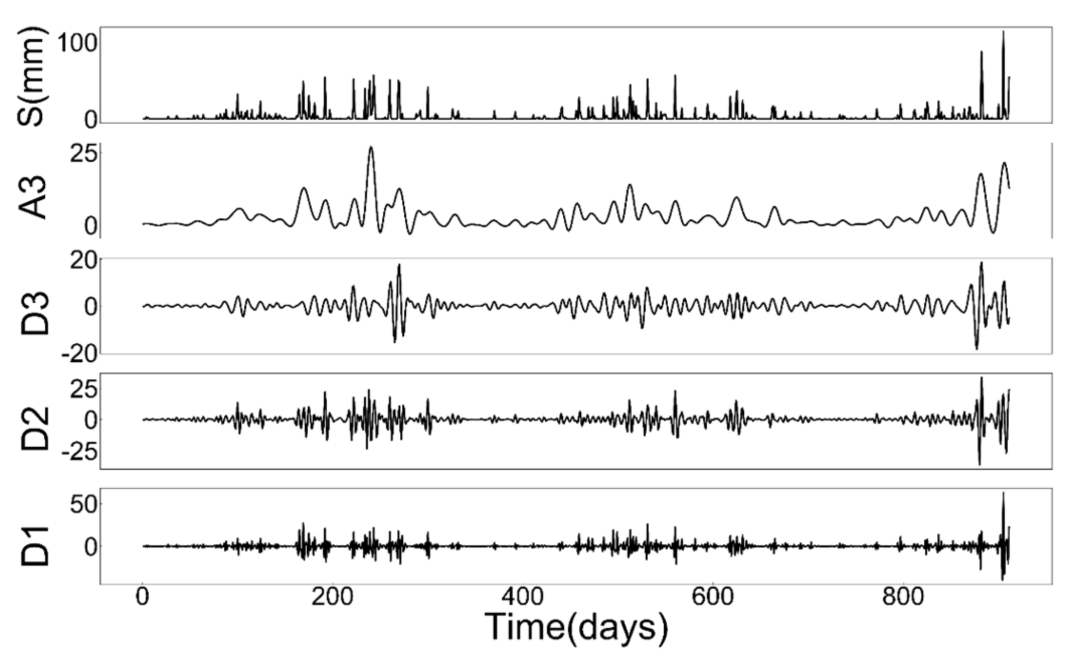
To verify the prediction accuracy of the DSP model proposed in this paper, we used data from station 57348 for rainfall prediction experiments. This station is located in Chongqing, China, with a subtropical, humid climate and abundant rainfall. The average annual rainfall at the station totals 881.9 mm over an average of 131 days. The distribution characteristics of the rainfall time series and the DWT decomposition results are shown in Figure 3. The final prediction results were obtained using the DSP model.
The SVR model was used to predict three high-frequency components (D1, D2, and D3), and the subsequence with the highest frequency D1 was used as an example for parameter selection (Table 3) and prediction (results in Figure 4). Figure 4 shows that the SVR model displays an excellent fitting ability for the high-frequency subsequence and yields satisfactory prediction results. The corresponding RMSE = 4.3709, MAE = 2.5513, and R2 = 0.6757.
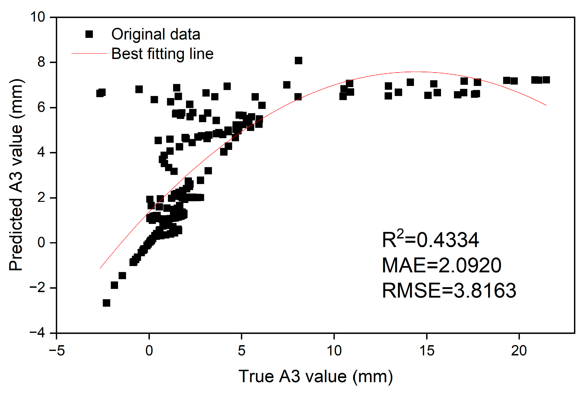
The Prophet model was applied to predict the low-frequency component A3, and the prediction results are shown in Figure 5. The resulting RMSE, MAE, and R2 were 3.8163, 2.0920, and 0.4334, respectively. The model can simulate the basic trend of A3, and the prediction results are within the acceptable range. The main parameters of the Prophet model are shown in Table 4.
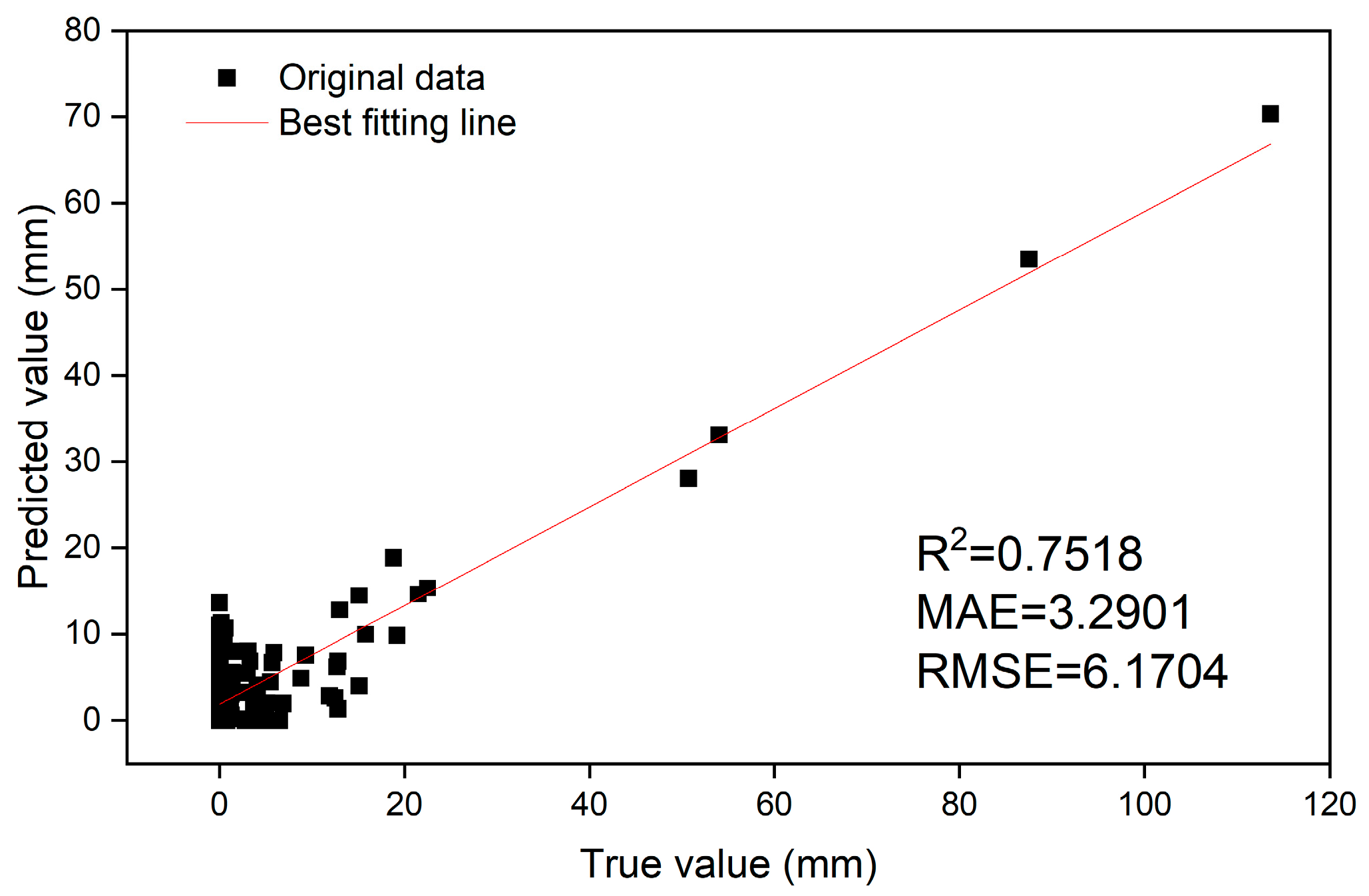
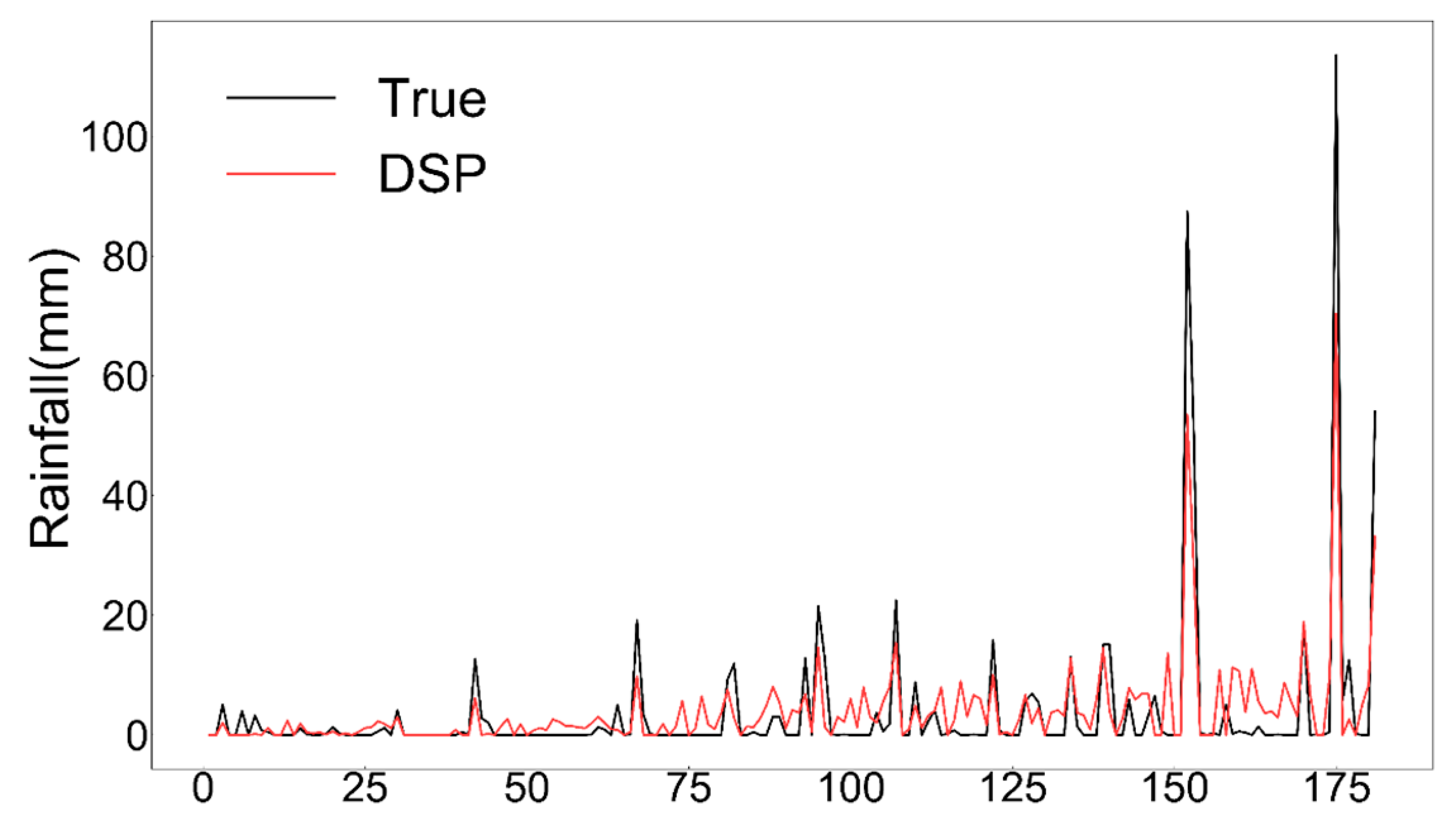
The prediction results of all components are summed to obtain the final prediction time series. Figure 6 shows the scatter plots of the real and predicted rainfall values based on the validation set, and Figure 7 compares the true and predicted values. The RMSE, MAE, and R2 of the DSP model are 6.1704, 3.2901, and 0.7518, respectively, indicating that among the studied models, the DSP model provides the best prediction of the basic trend of daily rainfall at station 57348. The predicted rainfall is generally similar to the actual rainfall, with satisfactory prediction accuracy.

3.2. The Prediction Accuracy of the DSP Model Is Higher Than That of the Baseline Models

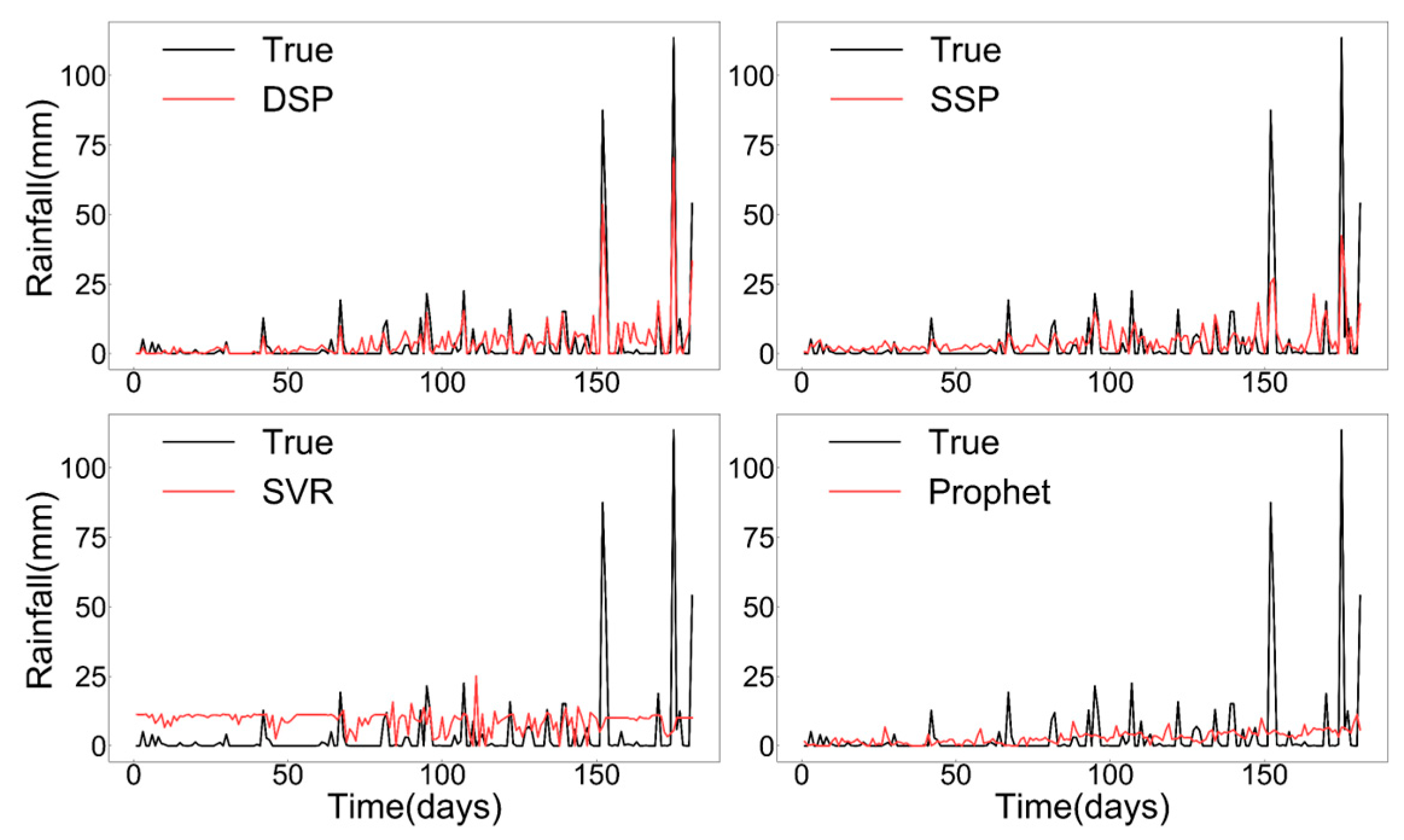
To validate the superiority of the DSP model, four experiments were conducted involving daily rainfall prediction at station 57348 using three baseline models and the DSP model. The three baseline models were the SVR, Prophet, and coupled SVR-Prophet models based on the seasonal decomposition method (SSP), proposed by Guo Li et al. [42]. The characteristics of these models are compared as shown in Table 5. The predicted and actual values of the four models based on the validation set are shown in Figure 8. The SVR and Prophet models have difficulty in predicting the true situation. The SVR model is influenced by extreme values and overpredicts rainfall. The Prophet model is weak in capturing extreme value changes and the prediction results fluctuate flatly. Notably, both the DSP model and the SSP model exhibit good performance. They can predict the variation of rainfall series better and the prediction results are close to the true values. The main difference is that the rainfall peak predicted by the SSP model is much lower than the observed value, and the corresponding prediction error is large. The DSP model displays better performance in fitting the detailed features of the rainfall series. The prediction accuracy of the four models was compared (Table 6), and the DSP model obtained the best evaluation results, followed by the SSP model. Compared with those of the SSP model, the RMSE and MAE of the DSP model were reduced by 46.3% and 55.9%, respectively, and the R2 was improved by 67.4%. The results above verify the superiority of the DSP model.
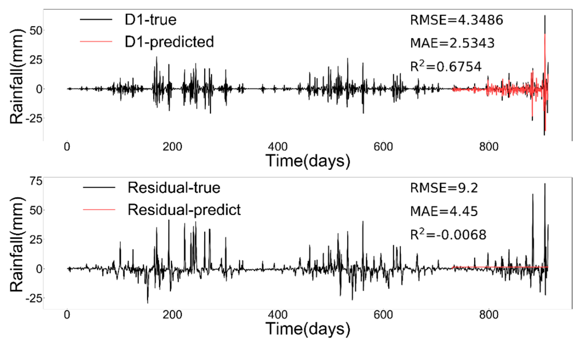
To further investigate the reasons for the difference in prediction effectiveness between the DSP model and the SSP model, comparative experiments are designed. The main difference between these two models is that when decomposing time series, the former uses discrete wavelet transform, while the latter uses seasonal decomposition to decompose time series. According to the principles of the decomposition methods, most of the detailed features of rainfall time series are associated with the high-frequency components in DWT and the residual terms in the Seasonal_decompose approach. Therefore, the rainfall data from station 57348 are used as an example, and the SVR model is applied to predict the D1 subsequence with the highest frequency in DWT and the residual term of Seasonal_decompose at the same time. Then, we compare the distribution characteristics and prediction results for components in detail, as shown in Figure 9. The prediction results of D1 fit the trend of the actual values, and good prediction performance is observed; in contrast, the prediction results based on the residual terms are poor, and variations in the components are not well predicted. D1 yields the smallest prediction error, with RMSE, MAE, and R2 values of 4.3486, 2.5343, and 0.6754, respectively. These findings indicate why the DSP model is superior to the SSP model in terms of peak rainfall prediction.

3.3. The DSP Model Displays Outstanding Stability

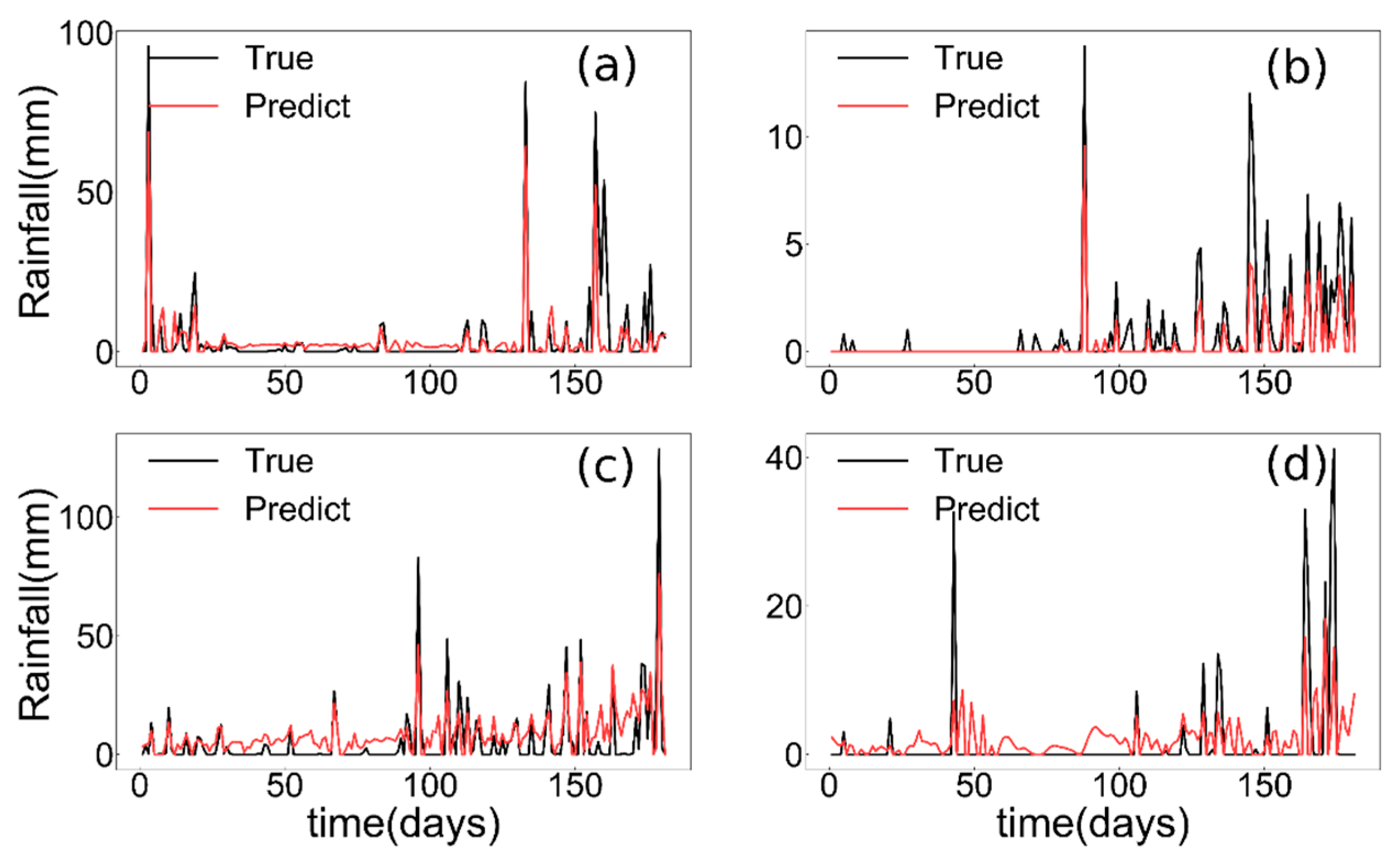
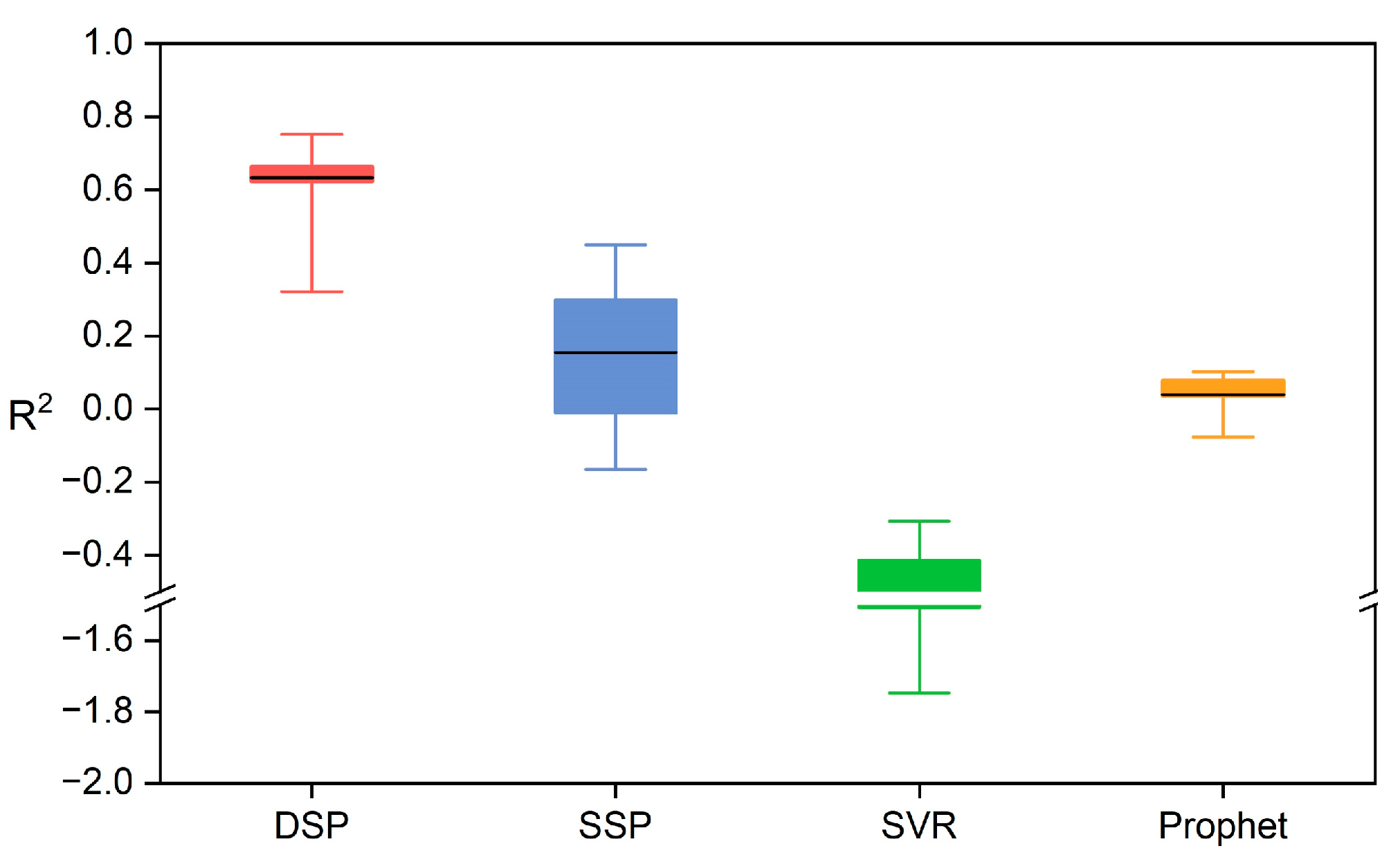
To evaluate the generalization ability of the DSP model, we conducted prediction experiments with data from stations in different climate zones. Additionally, we compared the prediction results of the DSP model with those of three baseline models. Figure 10 compares the predicted and true rainfall values at each station. The DSP model fits the general trend of data at different stations, and the prediction results are in good agreement with the actual values. The station-scale prediction accuracy metrics for the four models are given in Table 7. The ranges of RMSE and MAE of the DSP model are 1.24364 to 7.3116 and 0.5197 to 6.1431, respectively, and most R2 values range from 0.6217 to 0.7518. We select R2 as the evaluation index to further evaluate the performance of each model in different cases of rainfall prediction (see Figure 11). We found that most of the R2 values of the DSP model fluctuated slightly while remaining high at different stations. The R2 values of the SSP model were not stable and fluctuated considerably. Additionally, the R2 values of the Prophet and SVR models were consistently low. Therefore, compared with other baseline models, the DSP model displays the stronger generalization ability and yields stable prediction results.

4. Discussion

4.1. The DSP Model Achieves Accurate Forecasts of Rainfall Time Series

Since rainfall time series contain both periodic and nonstationary complex variations, hybrid methods are beneficial for overcoming the limitations of rainfall prediction [43]. Therefore, we propose a coupled DSP model for rainfall time series prediction and obtain satisfactory results (Figure 6 and Figure 7). Figure 8 shows that the DSP model exhibits the best prediction performance. The model accurately predicted the basic trends of the rainfall series and peak rainfall, and the predicted values generally matched the actual values. The Prophet model effectively fit the overall trend of the rainfall series, and the prediction curve was relatively flat, but the results of peak rainfall prediction were poor. The SVR model can capture the variation characteristics of rainfall series, but it is influenced by the peak rainfall, and the predicted values in some periods with little rainfall are much higher than the true values.
In previous studies, Malik et al. [44] used the SVR model to predict the effective drought index. Adaryani et al. [4] forecasted short-term rainfall with particle swarm optimization (PSO) and SVR. Hossain et al. [45] found that the Prophet model performed with better accuracy. The performance of these single models is recognized, but they cannot fit all features of hydrometeorological series. For example, the Prophet model can effectively fit the trend and period variations of time series, but the lack of consideration of residual autocorrelation leads to its poor fitting ability for complex models [42]. The SVR model displays good generalization ability and is suitable for nonlinear prediction; however, it has limitations for general data. By contrast, the DSP model successfully decomposes the periodic and nonstationary features in the rainfall time series using DWT and preserves them in different subseries. Moreover, the advantages of SVR and the Prophet model are combined in the DSP model to fit and predict subseries containing various features. Overall, the DSP model effectively fits the periodic and nonstationary factors in rainfall time series and achieves accurate predictions of rainfall time series.

4.2. The DSP Model Effectively Captures the Detailed Features of Rainfall Time Series

Achieving reliable predictions of rainfall time series is challenging, especially in the context of peak rainfall prediction [46]. Figure 8 illustrates the good prediction accuracy of the DSP model and the SSP model as well as the superior peak rainfall prediction capability of the DSP model. Based on the application of different data decomposition methods, Figure 9 compares the distribution characteristics and prediction effects of the components of the two models. The components obtained in DWT are generally associated with a single frequency and yield better prediction results than those in other cases. Notably, DWT is used to decompose time series while filtering some frequencies, making each component smoother. The excellent scale decomposition ability of DWT reduces the difficulty of fitting each component used in machine learning. After the extraction of trend and period terms, the residual terms in the Seasonal_decompose method are characterized by strong randomness and instability, thus limiting the performance of subsequent prediction models. Therefore, the DSP model based on DWT for data decomposition can best capture the detailed features of rainfall sequences and achieve accurate predictions of peak rainfall.

4.3. Generalization of DSP Models

Because the distribution characteristics of rainfall time series are influenced by the climate type, variations in the rainfall amplitude and frequency are impactful. Therefore, the rainfall time series from different climate types have different variation characteristics, affecting the results of prediction models. Multistation experiments involving the DSP model demonstrated its stable prediction ability (Figure 9). Table 5 and Figure 10 show that the DSP model yields high prediction accuracy at most stations. Only at station 54823 is there a significant decrease in accuracy, with an R2 of 0.3214. Although the prediction accuracy at this station is low, the trend of the prediction results is similar to the actual trend, and the predictions provide reference significance to some extent. At different stations, the DSP model produced reliable predictions, and the prediction accuracy was higher than that of the compared models. The above results fully verify that the DSP model provides outstanding prediction accuracy and stability in applications involving rainfall time series prediction. For other fields (e.g., the energy field, transportation field, and others), the complex time series of interest have the same characteristics as rainfall time series and contain both periodic and nonlinear variations. Theoretically, the DSP model can potentially achieve good performance in these fields and is worthy of further evaluation and application.

4.4. Disadvantages and Direction

The selection of the wavelet basis function and decomposition scale influences the fitting results during machine learning and the prediction performance of the DSP model. However, in this study, the wavelet basis function and decomposition level used in DWT are based on the previous study. Since we have yet to optimize the parameters of DWT, we cannot guarantee optimal decomposition. As shown in Figure 11, the prediction accuracy of the DSP model decreased for station 54823. This station is located in an area with a temperate monsoon climate, and the rainfall frequency is 20.7%, much lower than that at other stations. Thus, the DWT parameters used in this paper may not be suitable for station 54823 based on its unique rainfall data characteristics, leading to the failure of the DWT to achieve effective feature extraction and decomposition and thus affecting the prediction accuracy of the DSP model. Moreover, the prediction accuracy of the A1 component in Figure 5 is low, and there is a possibility that some high-frequency signals in the A1 component are not filtered, which affects the periodic fitting of the Prophet model. In subsequent work, the selection of DWT wavelet basis functions and decomposition levels for rainfall time series can be optimized with different features to adequately extract and decompose the different frequencies and characteristics of time series. The application of DWT decomposition after parameter optimization can further enhance machine learning and improve the accuracy and stability of rainfall time series prediction.

5. Conclusions

Accurate rainfall prediction is important to people’s production and life. The ability of the DWT-based coupled models to improve the accuracy of rainfall time series prediction is worthy of further study. In this paper, the DSP model is introduced for rainfall time series prediction. First, the DWT method is used to decompose the rainfall time series into high-frequency and low-frequency components. Then, the SVR model is used to predict the high-frequency components, and the Prophet model is used to predict the low-frequency components. Finally, the prediction results for each component are summed to obtain the final rainfall predictions.
The results of case studies show that the DSP model can accurately predict rainfall time series, with RMSE, MAE, and R2 values of 6.17, 3.29, and 0.75, respectively. The DSP model significantly improves the prediction accuracy, and the results are compared with those of the three baseline methods. Notably, the performances of the methods rank as follows: DSP > SSP > Prophet > SVR. Compared with the SSP model, the RMSE and MAE of the DSP model are reduced by 46.3% and 55.9%, respectively, and R2 is improved by 67.4%, verifying that the DSP model is an excellent prediction model. Moreover, the DSP model displays excellent prediction capability for peak rainfall events. The detailed feature prediction results of the DSP model display well, with RMSE = 4.35, MAE = 2.53, and R2 = 0.68. The DSP model also exhibits good generalization capability. The model achieves reliable predictions of rainfall time series with different features. The calculated RMSEs ranged from 1.24 to 7.31, the MAEs ranged from 0.52 to 6.14, and most R2 values ranged from 0.62 to 0.75. The DSP model can be applied in other fields in which time series are also periodic and nonstationary (e.g., the transportation and energy fields). Thus, the prediction performance of the DSP model deserves further study in additional applications.

Author Contributions

D.L. mainly contributed to drafting the manuscript, J.M. and H.Z. had the contribution of designing the whole research framework and drafting the manuscript, K.R. and X.W. were responsible for related data processing, and R.L. and Y.Y. contributed to the analysis. All authors commented on previous versions of the manuscript. All authors have read and agreed to the published version of the manuscript.

Funding

This work was supported by the National Key Research and Development Program of China (2022YFF1301803).

Data Availability Statement

The data that support the findings of this study are available from the first author upon reasonable request.

Acknowledgments

The authors are grateful for the funding support from the National Key Research and Development Program of China (2022YFF1301803).

Conflicts of Interest

The authors have no relevant financial or non-financial interest to disclose.

References

  1. Poornima, S.; Pushpalatha, M.; Jana, R.B.; Patti, L.A. Rainfall Forecast and Drought Analysis for Recent and Forthcoming Years in India. Water 2023, 15, 592. [Google Scholar] [CrossRef]
  2. Ni, L.; Wang, D.; Singh, V.P.; Wu, J.; Wang, Y.; Tao, Y.; Zhang, J. Streamflow and rainfall forecasting by two long short-term memory-based models. J. Hydrol. 2020, 583, 124296. [Google Scholar] [CrossRef]
  3. Rao, M.U.M.; Patra, K.C.; Sasmal, S.K.; Sharma, A.; Oliveto, G. Forecasting of Rainfall across River Basins Using Soft Computing Techniques: The Case Study of the Upper Brahmani Basin (India). Water 2023, 15, 499. [Google Scholar] [CrossRef]
  4. Adaryani, F.R.; Jamshid Mousavi, S.; Jafari, F. Short-term rainfall forecasting using machine learning-based approaches of PSO-SVR, LSTM and CNN. J. Hydrol. 2022, 614, 128463. [Google Scholar] [CrossRef]
  5. He, X.; Guan, H.; Qin, J. A hybrid wavelet neural network model with mutual information and particle swarm optimization for forecasting monthly rainfall. J. Hydrol. 2015, 527, 88–100. [Google Scholar] [CrossRef]
  6. Zhang, F.H.; Shao, Z.G. ST-GRF: Spatiotemporal graph neural networks for rainfall forecasting. Digit. Signal Process. 2023, 136, 103989. [Google Scholar] [CrossRef]
  7. Zhang, X.; Peng, Y.; Zhang, C.; Wang, B. Are hybrid models integrated with data preprocessing techniques suitable for monthly streamflow forecasting? Some experiment evidences. J. Hydrol. 2015, 530, 137–152. [Google Scholar] [CrossRef]
  8. Chong, K.L.; Lai, S.H.; Yao, Y.; Ahmed, A.N.; Jaafar, W.Z.W.; El-Shafie, A. Performance Enhancement Model for Rainfall Forecasting Utilizing Integrated Wavelet-Convolutional Neural Network. Water Resour. Manag. 2020, 34, 2371–2387. [Google Scholar] [CrossRef]
  9. Zhang, H.; Singh, V.P.; Wang, B.; Yu, Y. CEREF: A hybrid data-driven model for forecasting annual streamflow from a socio-hydrological system. J. Hydrol. 2016, 540, 246–256. [Google Scholar] [CrossRef]
  10. Nourani, V.; Hosseini Baghanam, A.; Adamowski, J.; Kisi, O. Applications of hybrid wavelet–Artificial Intelligence models in hydrology: A review. J. Hydrol. 2014, 514, 358–377. [Google Scholar] [CrossRef]
  11. Ojo, O.S.; Ogunjo, S.T. Machine learning models for prediction of rainfall over Nigeria. Sci. Afr. 2022, 16, e01246. [Google Scholar] [CrossRef]
  12. Karevan, Z.; Suykens, J.A.K. Transductive LSTM for time-series prediction: An application to weather forecasting. Neural Netw. 2020, 125, 1–9. [Google Scholar] [CrossRef]
  13. Aksoy, H.; Dahamsheh, A. Markov chain-incorporated and synthetic data-supported conditional artificial neural network models for forecasting monthly precipitation in arid regions. J. Hydrol. 2018, 562, 758–779. [Google Scholar] [CrossRef]
  14. Chen, L.; Sun, N.; Zhou, C.; Zhou, J.; Zhou, Y.; Zhang, J.; Zhou, Q. Flood Forecasting Based on an Improved Extreme Learning Machine Model Combined with the Backtracking Search Optimization Algorithm. Water 2018, 10, 1362. [Google Scholar] [CrossRef]
  15. Barrera-Animas, A.Y.; Oyedele, L.O.; Bilal, M.; Akinosho, T.D.; Delgado, J.M.D.; Akanbi, L.A. Rainfall prediction: A comparative analysis of modern machine learning algorithms for time-series forecasting. Mach. Learn. Appl. 2022, 7, 100204. [Google Scholar] [CrossRef]
  16. Liu, Z.; Zhou, P.; Chen, G.; Guo, L. Evaluating a coupled discrete wavelet transform and support vector regression for daily and monthly streamflow forecasting. J. Hydrol. 2014, 519, 2822–2831. [Google Scholar] [CrossRef]
  17. Aditya-Satrio, C.B.; Darmawan, W.; Nadia, B.U.; Hanafiah, N. Time series analysis and forecasting of coronavirus disease in Indonesia using ARIMA model and PROPHET. Procedia Comput. Sci. 2021, 179, 524–532. [Google Scholar] [CrossRef]
  18. Zhang, W.; Lin, Z.; Liu, X. Short-term offshore wind power forecasting—A hybrid model based on Discrete Wavelet Transform (DWT), Seasonal Autoregressive Integrated Moving Average (SARIMA), and deep-learning-based Long Short-Term Memory (LSTM). Renew. Energy 2022, 185, 611–628. [Google Scholar] [CrossRef]
  19. Vivas, E.; de Guenni, L.B.; Allende-Cid, H.; Salas, R. Deep Lagged-Wavelet for monthly rainfall forecasting in a tropical region. Stoch. Environ. Res. Risk Assess. 2023, 37, 831–848. [Google Scholar] [CrossRef]
  20. Samani, S.; Vadiati, M.; Delkash, M.; Bonakdari, H. A hybrid wavelet–machine learning model for qanat water flow prediction. Acta Geophys. 2022, 1–19. [Google Scholar] [CrossRef]
  21. Apaydin, H.; Taghi Sattari, M.; Falsafian, K.; Prasad, R. Artificial intelligence modelling integrated with Singular Spectral analysis and Seasonal-Trend decomposition using Loess approaches for streamflow predictions. J. Hydrol. 2021, 600, 126506. [Google Scholar] [CrossRef]
  22. Ravansalar, M.; Rajaee, T.; Kisi, O. Wavelet-linear genetic programming: A new approach for modeling monthly streamflow. J. Hydrol. 2017, 549, 461–475. [Google Scholar] [CrossRef]
  23. Samani, S.; Vadiati, M.; Nejatijahromi, Z.; Etebari, B.; Kisi, O. Groundwater level response identification by hybrid wavelet–machine learning conjunction models using meteorological data. Environ. Sci. Pollut. Res. 2023, 30, 22863–22884. [Google Scholar] [CrossRef]
  24. Xiang, Y.; Gou, L.; He, L.; Xia, S.; Wang, W. A SVR–ANN combined model based on ensemble EMD for rainfall prediction. Appl. Soft Comput. 2018, 73, 874–883. [Google Scholar] [CrossRef]
  25. Wang, H.; Wang, W.; Du, Y.; Xu, D. Examining the Applicability of Wavelet Packet Decomposition on Different Forecasting Models in Annual Rainfall Prediction. Water 2021, 13, 1997. [Google Scholar] [CrossRef]
  26. Wei, M.; You, X.Y. Monthly rainfall forecasting by a hybrid neural network of discrete wavelet transformation and deep learning. Water Resour. Manag. 2022, 36, 4003–4018. [Google Scholar] [CrossRef]
  27. Khan, M.M.H.; Muhammad, N.S.; El-Shafie, A. Wavelet based hybrid ANN-ARIMA models for meteorological drought forecasting. J. Hydrol. 2020, 590, 125380. [Google Scholar] [CrossRef]
  28. Adib, A.; Zaerpour, A.; Lotfirad, M. On the reliability of a novel MODWT-based hybrid ARIMA-artificial intelligence approach to forecast daily Snow Depth (Case study: The western part of the Rocky Mountains in the U.S.A). Cold Reg. Sci. Technol. 2021, 189, 103342. [Google Scholar] [CrossRef]
  29. He, R.; Zhang, L.; Chew, A.W.Z. Modeling and predicting rainfall time series using seasonal-trend decomposition and machine learning. Knowl.-Based Syst. 2022, 251, 109125. [Google Scholar] [CrossRef]
  30. Zhu, H.; Xu, R.; Deng, H. A novel STL-based hybrid model for forecasting hog price in China. Comput. Electron. Agric. 2022, 198, 107068. [Google Scholar] [CrossRef]
  31. Shamshirband, S.; Petković, D.; Javidnia, H.; Gani, A. Sensor Data Fusion by Support Vector Regression Methodology—A Comparative Study. IEEE Sens. J. 2015, 15, 850–854. [Google Scholar] [CrossRef]
  32. Huang, Y.-T.; Bai, Y.-L.; Yu, Q.-H.; Ding, L.; Ma, Y.-J. Application of a hybrid model based on the Prophet model, ICEEMDAN and multi-model optimization error correction in metal price prediction. Resour. Policy 2022, 79, 102969. [Google Scholar] [CrossRef]
  33. Luo, J.; Hong, T.; Fang, S.-C. Benchmarking robustness of load forecasting models under data integrity attacks. Int. J. Forecast. 2018, 34, 89–104. [Google Scholar] [CrossRef]
  34. Ponnoprat, D. Short-term daily precipitation forecasting with seasonally-integrated autoencoder. Appl. Soft Comput. 2021, 102, 107083. [Google Scholar] [CrossRef]
  35. Ma, Q.; Wang, H.; Luo, P.; Peng, Y.; Li, Q. Ultra-short-term Railway traction load prediction based on DWT-TCN-PSO_SVR combined model. Int. J. Electr. Power Energy Syst. 2022, 135, 107595. [Google Scholar] [CrossRef]
  36. Essam, Y.; Huang, Y.F.; Birima, A.H.; Ahmed, A.N.; El-Shafie, A. Predicting suspended sediment load in Peninsular Malaysia using support vector machine and deep learning algorithms. Sci. Rep. 2022, 12, 302. [Google Scholar] [CrossRef]
  37. Taylor, S.J.; Letham, B. Forecasting at Scale. Am. Stat. 2018, 72, 37–45. [Google Scholar] [CrossRef]
  38. Wu, C.; Zhang, X.; Wang, W.; Lu, C.; Zhang, Y.; Qin, W.; Tick, G.R.; Liu, B.; Shu, L. Groundwater level modeling framework by combining the wavelet transform with a long short-term memory data-driven model. Sci. Total Environ. 2021, 783, 146948. [Google Scholar] [CrossRef]
  39. Quilty, J.; Adamowski, J. A maximal overlap discrete wavelet packet transform integrated approach for rainfall forecasting—A case study in the Awash River Basin (Ethiopia). Environ. Model. Softw. 2021, 144, 105119. [Google Scholar] [CrossRef]
  40. Nalley, D.; Adamowski, J.; Khalil, B. Using discrete wavelet transforms to analyze trends in streamflow and precipitation in Quebec and Ontario (1954–2008). J. Hydrol. 2012, 475, 204–228. [Google Scholar] [CrossRef]
  41. Altunkaynak, A.; Nigussie, T.A. Prediction of daily rainfall by a hybrid wavelet-season-neuro technique. J. Hydrol. 2015, 529, 287–301. [Google Scholar] [CrossRef]
  42. Guo, L.; Fang, W.; Zhao, Q.; Wang, X. The hybrid PROPHET-SVR approach for forecasting product time series demand with seasonality. Comput. Ind. Eng. 2021, 161, 107598. [Google Scholar] [CrossRef]
  43. Fahad, S.; Su, F.; Khan, S.U.; Naeem, M.R.; Wei, K. Implementing a novel deep learning technique for rainfall forecasting via climatic variables: An approach via hierarchical clustering analysis. Sci. Total Environ. 2023, 854, 158760. [Google Scholar] [CrossRef] [PubMed]
  44. Malik, A.; Tikhamarine, Y.; Souag-Gamane, D.; Rai, P.; Sammen, S.S.; Kisi, O. Support vector regression integrated with novel meta-heuristic algorithms for meteorological drought prediction. Meteorol. Atmos. Phys. 2021, 133, 891–909. [Google Scholar] [CrossRef]
  45. Hossain, M.M.; Anwar, A.; Garg, N.; Prakash, M.; Bari, M. Monthly Rainfall Prediction at Catchment Level with the Facebook Prophet Model Using Observed and CMIP5 Decadal Data. Hydrology 2022, 9, 111. [Google Scholar] [CrossRef]
  46. Pihrt, J.; Raevskiy, R.; Šimánek, P.; Choma, M. WeatherFusionNet: Predicting Precipitation from Satellite Data. arXiv 2022, arXiv:2211.16824. [Google Scholar] [CrossRef]
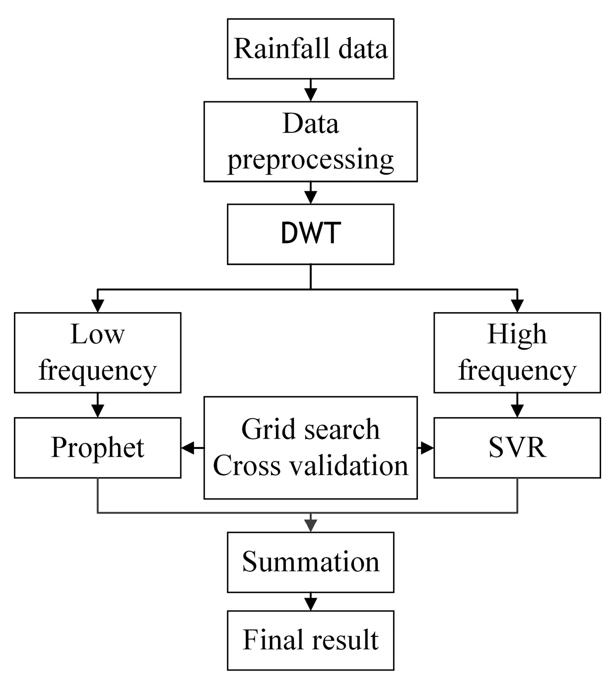
Figure 1. Main flowchart of the hybrid model.
Water 15 01935 g001
Figure 2. Time series decomposition process.
Water 15 01935 g002
Figure 3. Rainfall time series and its DWT decomposition results at station 57,348.
Water 15 01935 g003
Figure 4. Scatter plot of the predicted and true values of the D1 sequence.
Water 15 01935 g004
Figure 5. Scatter plot of the predicted and true values of the A3 sequence.
Water 15 01935 g005
Figure 6. Scatter plot of the predicted and true values of the rainfall time series.
Water 15 01935 g006
Figure 7. Comparison of the predicted and true rainfall time series.
Water 15 01935 g007
Figure 8. Comparison of the predicted and true rainfall time series using the DSP, SSP, SVR, and Prophet models at station 57348.
Water 15 01935 g008
Figure 9. Comparison of the predicted and true characteristics of the different components (D1 and residual terms).
Water 15 01935 g009
Figure 10. Comparison of the predicted and true values using the DSP model at different stations: (a) Station 59855; (b) Station 56018; (c) Station 58345; (d) Station 54823.
Water 15 01935 g010
Figure 11. Comparison of R2 values for four models based on predictions at different stations.
Water 15 01935 g011
Table 1. Rainfall data statistics.
Station (ID)Rainfall (mm)Rainfall Frequency
(%)
Climatic Type
Per YearPer MonthDaily
Maximum
Hainan (59855)1972.2182.6253.141.4Northern tropics
Jiangsu (58345)1362.7126.2154.836.0Northern subtropics
Chognqi (57348)881.981.7113.635.8Mid-subtropics
Shandon (54823)642.559.5127.120.7Southern temperate
Qinghai (56018)466.343.231.340.4Plateau climate
Table 2. Hyperparameters of the DWT, SVR, and Prophet models.
ModelParametersParameters DescriptionDefault ValueOptimization Method
DWTWavelet nameWavelet basis function-From
previous research
LevelWavelet decomposition level-
SVRKernelKernel functionrbfGrid search
CPenalty coefficient1
γKernel function coefficientauto
ProphetGrowthFunction in the trend modellinearGrid search
Changepoint_prior_scaleTrend flexibility0.05
Year_seasonalityYear flexibility10
Seasonality_prior_scaleSeasonality flexibility10
Seasonality modeModel learning styleadditive
Table 3. Parameter setting of the SVR model for the D1 sequence.
ParameterParameter Values
kernel functionrbf
C (penalty variable)1024
γ (kernel function parameter)0.03125
Table 4. Parameter setting of the Prophet model for the A3 sequence.
ParameterParameter Values
GrowthLinear
Changepoint_prior_scale1
Year_seasonality9
Seasonality_prior_scale60
Seasonality modeAdditive
Table 5. Comparison of the characteristics of the DSP, SSP, SVR, and Prophet models.
ModelAdvantagesDisadvantages
SVRIt displays good generalization ability and is suitable for nonlinear predictionIt has limitations for general data
ProphetIt can effectively fit the trend and period variations of time seriesPoor fitting ability for complex models
DSPIt can extract linear and nonlinear features and fit each component using dominance models, respectivelyThe parameter selection of DWT affects the prediction accuracy and requires additional optimization
SSPIt can extract linear and nonlinear features and fit each component using dominance models, respectivelyThe residual term is difficult to fit and requires high model performance
Table 6. Comparison of the prediction accuracy of the DSP, SSP, SVR, and Prophet models for rainfall at station 57348.
MetricDSPSSPSVRProphet
RMSE6.17049.167914.177912.1362
MAE3.29014.39319.57724.9510
R20.75180.4492−0.30610.0348
Table 7. Comparison of the prediction accuracy evaluation indexes for the different models at five stations in different climate regions.
StationMetricDSPSSPSVRProphet
59855RMSE7.311613.596119.948913.0716
MAE3.30357.491415.29084.4126
R20.6632−0.1647−1.5074−0.0766
56018RMSE1.23642.05192.93561.9336
MAE0.51970.91942.72190.9101
R20.6330−0.0107−1.06880.1024
58345RMSE8.839113.215117.082413.7878
MAE6.14318.055812.72097.1224
R20.62170.1543−0.41310.0794
54823RMSE4.85534.93679.77005.7756
MAE2.36432.87578.39832.4138
R20.32140.2985−1.74760.0398
57348RMSE6.17049.167914.177912.1362
MAE3.29014.39319.57724.9510
R20.75180.4492−0.30610.0348
Disclaimer/Publisher’s Note: The statements, opinions and data contained in all publications are solely those of the individual author(s) and contributor(s) and not of MDPI and/or the editor(s). MDPI and/or the editor(s) disclaim responsibility for any injury to people or property resulting from any ideas, methods, instructions or products referred to in the content.