Monte Carlo Simulation Approach to Shipping Accidents Consequences Assessment

Abstract

The purpose of this study is to present and apply an innovative technique to model environmental consequences of shipping accidents in relations to events initiating those accidents. The Monte Carlo simulation technique is used to model shipping accidents and chemical release consequences within the world’s sea and ocean waters. The model was created based on the previously designed novel general probabilistic approach to critical infrastructure accident consequences, including three models: the process of initiating events generated by a critical infrastructure accident, the process of environmental threats coming from released chemicals that are a result of initiating events, and the process of environmental degradation stemming from environmental threats. It is a new approach that has never been proposed and applied before. The Monte Carlo simulation method is used under the assumption of the semi-Markov model of these three processes. A procedure for the realization and generation of this process and evaluation of its characteristics is proposed and applied in the preparation of the C# program. Using this program, the processes’ characteristics are predicted for a specific sea area. Namely, for the considered processes, the limit values of transient probabilities between the states and the mean values of total sojourn times at the particular states for the fixed time are determined. The results obtained can be used practically by maritime practitioners involved in making decisions related to the safety of maritime transport and to mitigation actions concerned with maritime accidents.

1. Introduction

Shipping is one of the most-effective means of carrying huge amount of goods over long distances. It enables countries to trade and fosters their economic development. On the one hand, it is less dangerous to the environment than other means. On the other hand, constantly increasing traffic causes the risk of navigation hazards, despite the use of sophisticated supervising systems [1,2,3,4] and, consequently, the environmental impact of oil and other chemical releases [5,6,7]. Fortunately, despite the increase in transport intensity, the number of shipping accidents has decreased in recent decades [7]. About 90% of cargoes at the global scale are carried by sea. There are over 50,000 merchant ships around the world and a fleet is registered in more than 150 nations [8].

Transport on a general scale carries risks, including the risk of accidents. The reasons are different, although the human factor is dominant in each mode of transport [7,9]. Shipping accidents, such as collision, stranding, flooding, fire or explosion, are usually spectacular and may lead to serious consequences for the environment, its resources and seafarers [10,11,12]. Hull failures affecting the structural strength of the ship, damage to the ship’s equipment or system, loss of electrical or propulsion power, are some of the less threatening causes of accidents [13], but they may promote the next one, finally creating a chain of events [14]. The ships involved in marine accidents are mostly a means of transporting goods and/or people, thus pollution may be often significant, and even sometimes associated with a large number of victims. This is often complemented by large material losses, e.g., ship damage, high costs of rescue operations, closure of fisheries and recreation areas and mitigating of contamination effects [15,16,17,18,19].

According to a recent Allianz report on shipping losses and safety, there were 3000 accidents recorded around the world in 2021 and 54 of them resulted in the total loss of ship [20]. For comparison, Lloyd’s report points out that 21,746 accidents occurred in the years 2012–2020 and total loss of ships decreased from 132 in 2012 to 58 in 2020 [21]. Despite the fact that sea transport is most intensive within the Persian Gulf, west of the Atlantic Ocean, the Baltic Sea and in the north-west of the Pacific Ocean [22], regions of the North Sea, the English Channel, the British Isles, and the Bay of Biscay recorded the highest number (668) of marine accidents in 2021 [20]. Moreover, the sea areas around Indonesia, Indochina, Philippines and South China reported 1 in 5 total losses of ships in 2021 [20].

Modelling, identifying and analysing maritime transport risk play a crucial role in accident prevention. Fault trees, Bayesian networks, fuzzy logic and simulation are the most popular approaches to risk analysis and accident assessment [23,24,25,26,27,28,29,30,31,32,33]. Recently, the number of scientific research papers and publications on this topic has also increased [34]. The main focus of these studies is on the analysis of ship collisions and foundering, probably as casualties are the most frequent in these incidents, which represent together more than half of fatalities (57.4% in 2014–2021) [26,35]. For example, Monte Carlo simulation and the bidirectional long short-term memory neural network were used in a ship collision probability estimation model that allows the determination of the safety routes of ships [36]. Monte Carlo simulation combined with artificial neural network methods were also proposed in [37] to assess the probabilistic extent of damage in collision risk assessment and to predict the structural response to a ship collision. The probabilistic assessment of ship grounding evaluated by Monte Carlo simulation, and ship damage stability evaluation are proposed in [38]. Monte Carlo simulation has been for some years a commonly known technique in environmental risk assessment [39,40]. However, any of these approaches does not holistically investigate the problem of environmental consequences and losses caused by maritime accidents involving chemical releases, whilst simultaneously considering their initiating events. Currently, there are no competitive studies. The need of a mutual consideration of initiating events, environmental threats and environmental degradation in accident consequences analysis is obvious and very important for the maritime transport. Linking these three particular aspects is an original and novel approach to the analysis of the consequences of maritime accidents [41]. To the best of the authors’ knowledge, this study is among the first to use the Monte Carlo simulation technique to model shipping accidents in relation to their initiating events and chemical release consequences, not previously used in other studies. Therefore, the current proposal is different from other studies, in which causes and effects of accidents, such as aspects of marine pollution, are discussed separately. The new model was developed to analyse the data and evaluate the results in order to challenge existing practices.

A consistent nomenclature to highlight the key concepts and findings of the paper is presented in Appendix A,

Table A1. Glossary of technical terms and symbols.

Symbol	Description
IE	process of initiating events generated by a shipping critical infrastructure accident
ET	process of environmental threats coming from released chemicals that are a result of IE
ED	process of environmental degradation as a result of ET
$s^i$	realization of the process’ initial state at the moment t = 0
w	number of process’ states
${\mathsf{\Theta }}^{ij}$	random conditional sojourn times of a process at state $s^i$ when its next state is $s^j$
${\theta }^{ij}$	realization of the conditional sojourn time ${\mathsf{\Theta }}^{ij}$ of a process
$\tilde{\theta }$	experiment time
$n_{ij}$	number of sojourn time realizations during the time $\tilde{\theta }$
$H^{ij}\left(t\right)$	conditional distribution function of conditional sojourn time ${\mathsf{\Theta }}^{ij}$
${\left(H^{ij}\right)}^{-1}\left(h\right)$	inverse function of distribution function $H^{ij}\left(t\right)$
g, h	randomly generated numbers from the interval 〈0,1)
${\left[p^i\left(0\right)\right]}_{1\times \omega }$	vector of initial probabilities of a process at initial state $s^i$
${\left[p^{ij}\right]}_{\omega \times \omega }$	matrix of probabilities of transitions of a process between states $s^i$ and $s^j$
$p^i\left(t\right)$	transient probability of a process at state $s^i$ at the moment t
$p^i$	limit value of a transient probability $p^i\left(t\right)$
${\mathsf{\Theta }}^i$	unconditional sojourn time of a process at state $s^i$
$M^i$	mean value of unconditional sojourn time ${\mathsf{\Theta }}^i$ at state $s^i$
$\widehat{\theta }$	fixed time, e.g., 1 year to illustrate the results
${\widehat{\mathsf{\Theta }}}^i$	total sojourn time at state $s^i$, during the fixed time $\widehat{\theta }$
${\widehat{M}}^i$	mean value of total sojourn time ${\widehat{\mathsf{\Theta }}}^i$ at state $s^i$ during the fixed time
$N$	number of simulation iterations
$RE$	relative error between simulation and analytical expected values

. It consists of technical terms and concepts used in Section 2, Section 3 and Section 4.

2. Materials and Methods

The general model of critical infrastructure accident consequences (CIAC) is described in [41]. The CIAC consists of three models:

• the process of initiating events (IE) generated by a critical infrastructure accident;
• the process of environmental threats (ET) coming from dangerous situations in the critical infrastructure operating area that are a result of IE;
• the process of environmental degradation (ED) as a result of environmental threats (ET).

Next, the semi-Markov models of these processes [42,43,44,45,46,47] are considered jointly. To do this, it is assumed that the ET process is conditional. This means that the ET process involves the process of IE, because the ET process depends on the IE process. Similarly, the ED process is conditional, as its states depend on the states of the ET process [48,49,50]. These interdependencies are discussed in more detail in Section 2.1, Section 2.2 and Section 2.3 and presented in Figure 1.

The probabilistic general model of CIAC, which is made up of the three models mentioned above, is adopted within the world’s sea waters, using statistical historical accident data. Here, the CIAC model is used for identification and prediction of the environmental accident consequences generated by ships belonging to networks operating globally. The background parameters of these processes are described below. Next, the Monte Carlo simulation technique, based on the stochastic general model, is applied. First, using self-written software in C#, a simulation procedure is proposed and applied to generate the realization of the three processes and evaluate their characteristics, predicted for the considered sea area. Specifically, the limit values of transient probabilities and the mean values of total sojourn times for the pre-set time at the fixed states are determined.

2.1. General Model of Shipping Accident and Chemical Release Consequences

The general model of shipping accident and chemical release consequences is created, based on the probabilistic approach of CIAC, including three models as three connected processes [41]:

• the process of IE generated by a shipping critical infrastructure accident;
• the ET process stemming from released chemicals that are a result of IE;
• the ED process as a result of ET.

In the following Section 2.1.1, Section 2.1.2 and Section 2.1.3, the semi-Markov models of these three (IE, ET and ED) processes are distinguished. To model the processes, a time interval $t\in ⟨0,+\infty )$ is assumed for the ship’s operation within global sea waters, and the appropriate designations and notions are distinguished.

2.1.1. Process of Initiating Events (IE)

The basic designations are introduced to define the process of IE:

• the number $n_1,$ where $n_1\in N$, of events initiating a dangerous situation for the ship operating in the specific environment;
• kinds of IE: $E_1,E_2,\dots ,E_{n_1};$
• the number of IE states $\omega ,$ $\omega \in N;$
• IE states $e^l=\left[e_1^l,e_2^l,\dots ,e_{n_1}^l\right],$ where $e_i^l\in \left\{\mathrm{0,1}\right\}$, $l=\mathrm{1,\; 2},\dots ,\omega ,$ $i=\mathrm{1,\; 2},\dots ,n_1;$
• the process of IE: $E\left(t\right)$ with states from the set $E=\left\{e^1,e^2,\dots ,e^{\omega }\right\};$
• the probabilities $p^{lj},$ $l,j=\mathrm{1,\; 2},\dots ,\omega ,$ $l\ne j$ of transitions between the different states $e^l$ and $e^j;$
• random conditional sojourn times ${\theta }^{lj}$ at the state $e^l$ while the next transition will be performed for the different state $e^j;$
• the conditional distribution functions $H^{lj}\left(t\right)=P\left({\theta }^{lj}<t\right)$ of ${\theta }^{lj}$ at the state $e^l$ while the next transition will be performed for the state $e^j.$

The main characteristics for the process of IE are:

• the limit transient probabilities $p^l$ of the probabilities $p^l\left(t\right)=P\left(E\left(t\right)=e^l\right)$ remaining at the states $e^l$;
• the mean values ${\widehat{M}}^l=E\left[{\widehat{\theta }}^l\right]\cong p^l\theta$ of the sojourn total times ${\widehat{\theta }}^l$ in the time interval $〈0,\theta 〉,\theta >0$ at particular states $e^l$.

2.1.2. Process of Environmental Threats (ET)

The basic designations are introduced to define the ET process:

• the number $n_2,$ where $n_2\in N$, of kinds of threats that may cause environmental degradation;
• kinds of environmental threats: $H_1,H_2,\dots ,H_{n_2}$;
• factors $f^1,f^2,\dots ,f^{n_2}$ characterising the environmental threats;
• the number $l^i$, where $l^i\in N$, $i=\mathrm{1,\; 2},\dots ,n_2$, of factors’ values ranges;
• ranges $f^{i1},f^{i2},\dots ,f^{{il}^i}$ of factors’ values;
• the number $n_3,$ where $n_3\in N$ of environment sub-areas;
• environment sub-areas $D_1,D_2,\dots ,D_{n_3}$ of the ship operating within the environment area $D=D_1\cup D_2\cup \dots \cup D_{n_3}$ that may be degraded by the environmental threats;
• the conditional process $S_{(k/l)}\left(t\right)$ of ET in the subarea $D_k,$ $k=\mathrm{1,\; 2},\dots ,n_3$, while the process of IE is at the state $e^l$;
• the process $S_{\left(k\right)}\left(t\right)$ of ET in the sub-area $D_k,$ $k=\mathrm{1,\; 2},\dots ,n_3$;
• the number of ET states ${\upsilon }_k,$ ${\upsilon }_k\in N$ of the sub-area;
• ET states $s_{\left(k\right)}^{\upsilon }=\left[f_{\left(k\right)}^1,f_{\left(k\right)}^2,\dots ,f_{\left(k\right)}^{n_2}\right],$ where $f_{\left(k\right)}^i\in \left\{0,f_{\left(k\right)}^{ij}\right\}$, $i,j,\upsilon =\mathrm{1,\; 2},\dots ,{\upsilon }_k,$ $k=\mathrm{1,\; 2},\dots ,n_3$, $s_{\left(k\right)}^i\ne s_{\left(k\right)}^j$, for $i\ne j$;
• the probabilities $p_{(k/l)}^{ij},$ $l,j=\mathrm{1,\; 2},\dots ,{\upsilon }_k,$ $l\ne j$ of transitions between the different states $s_{(k/l)}^i$ and $s_{(k/l)}^j$;
• random conditional sojourn times ${\eta }_{(k/l)}^{ij}$ at the state $s_{(k/l)}^i$ while the next transition will be performed for the different state $s_{(k/l)}^j$;
• the conditional distribution functions $H_{(k/l)}^{ij}\left(t\right)=P\left({\eta }_{(k/l)}^{ij}<t\right)$ of ${\eta }_{(k/l)}^{ij}$ at the state $s_{(k/l)}^i$ while the next transition will be performed for the state $s_{(k/l)}^j.$

The main characteristics for the conditional ET process are:

• the limit transient probabilities $p_{(k/l)}^i$ of the probabilities $p_{\left(k/l\right)}^i\left(t\right)=P(S_{(k/l)}\left(t\right)=s_{(k/l)}^i)$ remaining at the states $s_{(k/l)}^i$;
• the mean values ${\widehat{M}}_{(k/l)}^i=E\left[{\widehat{\eta }}_{(k/l)}^i\right]\cong p_{(k/l)}^i\eta$ of the sojourn total times ${\widehat{\eta }}_{(k/l)}^i$ in the time interval $〈0,\eta 〉,$ $\eta >0$ at particular states $s_{(k/l)}^i$.

The main characteristic for the unconditional process $S_{\left(k\right)}\left(t\right)$ is:

• the limit transient probabilities $p_{\left(k\right)}^i$ of the probabilities $p_{\left(k\right)}^i\left(t\right)=\sum _{l=1}^{\omega }P\left(E\left(t\right)=e^l\right)·P\left(S_{\left(k\right)}\left(t\right)=s_{\left(k\right)}^i|E\left(t\right)=e^l\right)=\sum _{l=1}^{\omega }{p}^l\left(t\right)·p_{(k/l)}^i\left(t\right)$ remaining at the states $s_{\left(k\right)}^i$ are given by

  $$p_{\left(k\right)}^i=\sum _{l=1}^{\omega }{p}^l·p_{(k/l)}^i,i=\mathrm{1,\; 2},\dots ,{\upsilon }_k,k=\mathrm{1,\; 2},\dots ,n_3$$

  (1)

  where $p^l$ and $p_{(k/l)}^i$ are mentioned earlier.

2.1.3. Process of Environmental Degradation (ED)

The basic designations to define the ED process are introduced:

• the number $m_k,$ where $m_k\in N$, of dangerous degradation effects for the environment subarea $D_k,$ $k=\mathrm{1,\; 2},\dots ,n_3$;
• degradation effects $R_{\left(k\right)}^1,R_{\left(k\right)}^2,\dots ,R_{\left(k\right)}^{m_k}$;
• states of the degradation effect $R_{\left(k\right)}^m$, which are the levels $R_{\left(k\right)}^{m1},R_{\left(k\right)}^{m2},\dots ,R_{\left(k\right)}^{m{\nu }_{\left(k\right)}^m}$, $m=\mathrm{1,\; 2},\dots ,m_k$;
• the number ${\nu }_{\left(k\right)}^m$, ${\nu }_{\left(k\right)}^m\in N$, of degradation effect levels;
• the number of ED states ${\ell }_k,$ ${\ell }_k\in N$ of the sub-area;
• ED states $r_{\left(k\right)}^m=\left[d_{\left(k\right)}^1,d_{\left(k\right)}^2,\dots ,d_{\left(k\right)}^{m_k}\right],$ in the sub-area, where $d_{\left(k\right)}^m\in \left\{0,R_{\left(k\right)}^{mj}\right\}$, $j=\mathrm{1,\; 2},\dots {\nu }_{\left(k\right)}^m$;
• ED states $R_{\left(k\right)}=\left\{r_{\left(k\right)}^{\ell },\ell =\mathrm{1,\; 2},\dots ,{\ell }_k\right\},$ in the sub-area, when some of the states $r_{\left(k\right)}^m$ cannot occur, where $d_{\left(k\right)}^m\in \left\{0,R_{\left(k\right)}^{mj}\right\}$, $j=\mathrm{1,\; 2},\dots {\nu }_{\left(k\right)}^m,$ $r_{\left(k\right)}^i\ne r_{\left(k\right)}^j$, for $i\ne j$;
• the conditional process $R_{(k/\upsilon )}\left(t\right)$ of ED in the sub-area $D_k,$ $k=\mathrm{1,\; 2},\dots ,n_3$, $\upsilon =\mathrm{1,\; 2},\dots ,{\upsilon }_k$, while the process of environmental threats $S_{\left(k\right)}\left(t\right)$ is at the state $s_{\left(k\right)}^{\upsilon },$ $\upsilon =\mathrm{1,\; 2},\dots ,{\upsilon }_k,$ $k=\mathrm{1,\; 2},\dots ,n_3$ and having values in the environmental degradation states set;
• the process $R_{\left(k\right)}\left(t\right)$ of ED in the sub-area $D_k,$ $k=\mathrm{1,\; 2},\dots ,n_3$, involved with the process of environmental threats $S_{\left(k\right)}\left(t\right)$;
• the probabilities $q_{(k/\upsilon )}^{ij},$ $i,j=\mathrm{1,\; 2},\dots ,{\ell }_k,$ $i\ne j$ of transitions between the different states $r_{(k/\upsilon )}^i$ and $r_{(k/\upsilon )}^j$;
• random conditional sojourn times ${\zeta }_{(k/\upsilon )}^{ij}$ at the state $r_{(k/\upsilon )}^i$ while the next transition will be performed for the different state $r_{(k/\upsilon )}^j$;
• the conditional distribution functions $G_{(k/\upsilon )}^{ij}\left(t\right)=P\left({\zeta }_{(k/\upsilon )}^{ij}<t\right)$ of ${\zeta }_{(k/\upsilon )}^{ij}$ at the state $r_{(k/\upsilon )}^i$ while the next transition will be performed for the state $r_{(k/\upsilon )}^j.$

The main characteristics for the process $R_{(k/\upsilon )}\left(t\right)$ are:

• the limit transient probabilities $q_{(k/\upsilon )}^i$ of the probabilities $q_{\left(k/\upsilon \right)}^i\left(t\right)=P(R_{(k/\upsilon )}\left(t\right)=r_{(k/\upsilon )}^i)$ remaining at the states $r_{(k/\upsilon )}^i$;
• the mean values ${\widehat{M}}_{(k/\upsilon )}^i=E\left[{\widehat{\zeta }}_{(k/\upsilon )}^i\right]\cong q_{(k/\upsilon )}^i\zeta$ of the sojourn total times ${{\widehat{\zeta }}^i}_{(k/v)}$ in the time interval $〈0,\zeta 〉,$ $\zeta >0$ at particular states $r_{(k/\upsilon )}^i$.

The main characteristic for the process $R_{\left(k\right)}\left(t\right)$ is:

• the limit transient probabilities $q_{\left(k\right)}^i$ of the probabilities $q_{\left(k\right)}^i\left(t\right)=\sum _{\upsilon =1}^{{\upsilon }_k}P\left(S\left(t\right)=s_{\left(k\right)}^{\upsilon }\right)·P\left(R_{\left(k\right)}\left(t\right)=r_{\left(k\right)}^i|S\left(t\right)=s_{\left(k\right)}^{\upsilon }\right)=\sum _{\upsilon =1}^{{\upsilon }_k}{p}_{\left(k\right)}^{\upsilon }\left(t\right)·q_{(k/\upsilon )}^i\left(t\right)$ remaining at the states $r_{\left(k\right)}^i$, given by

  $$\begin{gathered} q_{\left(k\right)}^i=\sum _{\upsilon =1}^{{\upsilon }_k}{p}_{\left(k\right)}^{\upsilon }·q_{\left(k/\upsilon \right)}^i=\sum _{\upsilon =1}^{{\upsilon }_k}\left[\sum _{l=1}^{\omega }{p}^l·p_{(k/l)}^{\upsilon }\right]q_{\left(k/\upsilon \right)}^i, \\ i=\mathrm{1,\; 2},\dots ,{\ell }_k,k=\mathrm{1,\; 2},\dots ,n_3 \end{gathered}$$

  (2)

  where $p^l,$ $p_{(k/l)}^i$ and $q_{(k/\upsilon )}^i$ are mentioned earlier.

The Formula (2) expresses the limit forms of total probabilities of the joint (superposition) processes: IE, ET and ED.

The interdependencies of the particular processes from which the joint model of CIAC is composed are presented in Figure 1.

2.2. Monte Carlo Simulation-Based General Model of Shipping Accident and Chemical Release Consequences

In this Section, a model of shipping accident and chemical release consequences, based on the designed general probabilistic approach of critical infrastructure accident consequences, is presented. This paper proposes a non-analytical, approximate approach, i.e., a computer simulation technique based on the Monte Carlo method. This method can provide fairly accurate results in a relatively short time spent on calculations.

In order to estimate the unknown basic parameters of the processes IE, ET and ED, firstly the number of states of the processes should be fixed and the states should be defined. Next, the numbers of transients from one state to another should be counted, at the initial moment (starting point), as well as during the experiment time.

After the statistical data collection, i.e., numbers of initial states, numbers of transitions between the states and the conditional sojourn times’ realizations, the identification of statistical parameters is carried out. Namely, the initial probabilities, the probabilities of transitions between the states and the hypotheses on the distribution functions of that random conditional sojourn times were verified. When the basic parameters are identified, it is possible to fix the input data for Monte Carlo simulation, assuming the initial time t = 0.

2.2.1. Generating Processes’ Basic Parameters

The general model of shipping accident and chemical release consequences consists of three processes: IE, ET and ED (see Section 2.1). Each of those processes is defined by the initial probabilities at its states, the probabilities of transitions between these states and the distributions of the conditional sojourn times at these states in Section 2.1.1, Section 2.1.2 and Section 2.1.3. Next, the main characteristics of the considered processes, i.e., the limit values of transient probabilities and the unconditional mean values of total sojourn times at the particular states for the fixed time, can be determined. The procedure for obtaining these characteristics is presented in Section 2.2.2.

Moreover, these results are used to perform the superposition of three particular processes: IE, ET and ED, according to (2), also illustrated in Figure 1.

2.2.2. Monte Carlo Simulation Procedure for Processes’ Characteristics Determination

A procedure for the processes’ generation of realizations and evaluation of its characteristics is proposed. This procedure can be applied for all three processes, thus the denotations are general, and not exactly the same as in Section 2.1.1, Section 2.1.2 and Section 2.1.3.

To conduct the simulation, the formulae for generating the initial state of the process, and the next states it stays at, are introduced. The nomenclature is presented in Appendix A.

The realization of the process’ initial state at the moment t = 0 is denoted by $s^i=s^i\left(g\right)$, $i\in \left\{\mathrm{1,\; 2},\dots ,\omega \right\}$. Further, the state is selected by generating realizations from the distribution defined by the vector ${\left[p^i\left(0\right)\right]}_{1\times \omega },$ according to the formula

$$s^i\left(g\right)=s^b,\sum _{\rho =1}^b{p}^{\rho -1}\left(0\right)\le g<\sum _{\rho =1}^b{p}^{\rho }\left(0\right),b\in \left\{\mathrm{1,\; 2},\dots ,\omega \right\},$$

(3)

where $g$ is a randomly generated number from the uniform distribution on the interval 〈0,1) and $p^0\left(0\right)=$ 0.

After selecting the initial state $s^i,$ $i\in \left\{\mathrm{1,\; 2},\dots ,\omega \right\}$, the next state of the process can be fixed. The sequence of the realizations of the consecutive states of the process generated from the distribution defined by the matrix ${\left[p^{ij}\right]}_{\omega \times \omega }$ are denoted by $s^j=s^j\left(g\right)$, $j\in \left\{\mathrm{1,\; 2},\dots ,\omega \right\},$ $j\ne i$. These realizations are generated for a fixed i, $i\in \left\{\mathrm{1,\; 2},\dots ,\omega \right\},$ according to the formula

$$\begin{gathered} s^j\left(g\right)=s^l,\sum _{\rho =1}^l{p}^{j(\rho -1)}\le g<\sum _{\rho =1}^l{p}^{j\rho }, \\ l\in \left\{\mathrm{1,\; 2},\dots ,\omega \right\},l\ne i \end{gathered}$$

(4)

where g is a randomly generated number from the uniform distribution on the interval 〈0,1) and $p^{i0}=$ 0.

After selecting the initial state and the next state, the time for staying in the state (sojourn time) can be generated randomly from a given distribution function. In other words, first a pseudo-random number g is drawn by a computer program and the initial state is generated according to (3). Then, the program draws another pseudo-random number g and generates a next state according to (4). For instance, if the first state is $s^i=$ 3 and the next state is $s^j=$ 4, then the program will generate the conditional sojourn time from the distribution of the random variable ${\mathsf{\Theta }}^{34}$ (representing the time staying in a state 3, under the condition that the next state will be 4).

The inverse transform method (also known as inversion sampling method) can be used for generating draws from a given probability distribution. This is convenient if it is possible to determine the inverse distribution function [42,43,44,51,52,53,54].

To receive a sufficient number of realizations of the considered random conditional sojourn time ${\mathsf{\Theta }}^{ij}$, $i,j=\mathrm{1,\; 2},\dots ,v,$ $i\ne j$, is denoted by ${\theta }^{ij}$, the realizations at the state $s^i$, while the next transition will be carried out for the different state $s^j$. These realizations are generated from the distribution $H^{ij}$, where $n_{ij}$ is the number of the sojourn time realizations during the fixed experiment time $\tilde{\theta }$, according to the formula

$${\theta }^{ij}={\left(H^{ij}\right)}^{-1}\left(h\right),$$

(5)

where ${\left(H^{ij}\right)}^{-1}\left(h\right)$ is the inverse function of the distribution function $H^{ij}\left(t\right)$ and $h$ is a randomly generated number from the uniform distribution on the interval (0,1〉.

The realizations are numerated

$${\theta }_{\left(1\right)}^{ij},{\theta }_{\left(2\right)}^{ij},\dots ,{\theta }_{\left(n_{ij}\right)}^{ij}$$

(6)

for the conditional sojourn times of the process and it is possible to determine approximately the total sojourn time at the state $s^i$ during the time of the experiment $\tilde{\theta }$ applying the formula

$${\tilde{\theta }}^i=\sum _{\begin{array}{c}j=1\\ j\ne i\end{array}}^v\sum _{\rho =1}^{n^{ij}}{\theta }_{\left(\rho \right)}^{ij}.$$

(7)

Further, the limit transient probabilities $p^i\left(t\right)$ can be approximately obtained using the formula

$$p^i=\frac{{\tilde{\theta }}^i}{\tilde{\theta }}$$

(8)

where

$$\tilde{\theta }=\sum _{i=1}^v{\tilde{\theta }}^i.$$

(9)

The mean values of the process’ unconditional sojourn times ${\mathsf{\Theta }}^i$ at the particular states are given respectively by

$$M^i=\frac{1}{n_i}{\tilde{\theta }}^i,n_i=\sum _{j=1}^w{n}_{ij},i\in \left\{\mathrm{1,\; 2},\dots ,\omega \right\}.$$

(10)

Other interesting characteristics of the process are its total sojourn times ${\widehat{\mathsf{\Theta }}}^i$ at the particular states $s^i$, during the fixed time $\widehat{\theta }$. It is well known [42,44,45] that the total sojourn time ${\widehat{\mathsf{\Theta }}}^i$ of the process at the state $s^i$, $i\in \left\{\mathrm{1,\; 2},\dots ,\omega \right\},$ for a sufficiently large time, has approximately normal distribution, with the expected value given as follows

$${\widehat{M}}^i=E[{\widehat{\mathsf{\Theta }}}^i]=p^i·\widehat{\theta }, i\in \left\{\mathrm{1,\; 2},\dots ,\omega \right\}.$$

(11)

The following detailed procedure is formed and applied in C# program preparation.

Procedure 1.

Monte Carlo simulation procedure to estimate process characteristics.

• Draw a randomly generated number $g$ from the uniform distribution on the interval (0,1〉;
• Select the initial state $s^i$, $i\in \{\mathrm{1,\; 2},\dots ,\omega \}$, according to (3);
• Draw another randomly generated number $g$ from the uniform distribution on the interval (0,1〉;
• For the fixed $i$, select the next state $s^j$, $j\in \{\mathrm{1,\; 2},\dots ,\omega \}$, $j\ne i$, according to (4);
• Draw a randomly generated number $h$ from the uniform distribution on the interval (0,1〉;
• For the fixed $i$ and $j$, generate a realization ${\theta }^{ij}$, of the conditional sojourn time ${\mathsf{\Theta }}^{ij}$, from a given probability distribution, according to (5);
• Substitute $i:=j$ and repeat 3.–6., until the sum of all generated realizations ${\theta }^{ij}$ reaches a fixed experiment time $\tilde{\theta }$;
• Calculate total sojourn times at the states $s^i$, according to (7);
• Calculate limit transient probabilities at the particular states $s^i$, according to (8);
• Calculate unconditional mean sojourn times at the states $s^i$, according to (10);
• Calculate mean values of the total sojourn times at the states $s^i$, during the fixed time $\widehat{\theta }$, according to (11).

The procedure is used to prepare a C# program code and, further, using the statistical data, the processes’ characteristics are predicted (Section 3). The limit values of transient probabilities and the mean values of total sojourn times for the fixed time at the fixed states are evaluated.

2.3. Sources of Real Data

The model is adopted to the maritime transport critical infrastructure, understood as a ship network operating in sea waters, using the statistical data on sea accidents occurring in global sea waters in 2004–2014. These data come from freely accessible databases: the Global Integrated Shipping Information System Centre of Documentation—GISIS, and the Research and Experimentation on Accidental Water Pollution—CEDRE (available on the websites: www.cedre.fr and https://webaccounts.imo.org respectively, accessed on 13 July 2022). Namely, 1630 reports collected on ship casualties are analysed and an 11 years period is considered as the experimental time for this research.

The initiating events, the environmental threats and environmental degradation effects are defined and background parameters are described, similarly to those distinguished by maritime authorities such as the International Maritime Organization.

The necessary statistical data for the processes are collected and processed, and the hypotheses concerned with the distributions of the random conditional sojourn times are formulated and verified. These results are described in [41,48,49,50]. After performing the identification, it is possible to process the data and predict the processes’ basic characteristics (see Section 3.2).

In Section 3, Section 4 and Section 5, a description is given to illustrate the results clearly.

3. Results

Using the statistical data from the CEDRE and the GISIS mentioned in Section 2.3, the initiating events and environmental degradation as consequences of sea accidents and chemical releases are identified and predicted for the world’s sea waters.

3.1. Modelling Shipping Accident Consequences

3.1.1. Modelling the Process of IE

The initiating events are the fundamentals of the model of the process of IE [13,41], as follows:

• $E_1$—collision;
• $E_2$—grounding;
• $E_3$—contact with an external object;
• $E_4$—fire or explosion on a board;
• $E_5$—shipping without control (drifting, or missing ship);
• $E_6$—capsizing or listing of a ship;
• $E_7$—movement of cargo in a ship.

The states of the process of IE are based on the types of IE mentioned above and expressed by vectors, where 0 means that any IE dangerous to the environment does not appear and 1 means that IE appears. For instance, the vector $e^1=$ [0,0,0,0,0,0,0] expresses no initiating event occurred, the vector $e^5=$ [0,0,0,1,0,0,0] expresses the initiating event $E_4$(fire or explosion on a board) occurred, and the vector $e^9=$ [0,1,0,1,0,0,0] expresses both the initiating event $E_2$(grounding) and the initiating event $E_4$(fire or explosion on a board) occurred.

Further, the vectors that did not occur within the considered experimental time are eliminated and the remaining ones are numbered. In this way, $\omega =$16 numbers of IE states are defined and presented in Appendix B,

Table A2. States of process of IE.

IE State	Type of IE *
	E1	E2	E3	E4	E5	E6	E7
e1	0	0	0	0	0	0	0
e2	1	0	0	0	0	0	0
e3	0	1	0	0	0	0	0
e4	0	0	1	0	0	0	0
e5	0	0	0	1	0	0	0
e6	0	0	0	0	1	0	0
e7	0	0	0	0	0	1	0
e8	0	0	0	0	0	0	1
e9	0	1	0	1	0	0	0
e10	0	0	0	1	1	0	0
e11	0	0	0	0	1	1	0
e12	0	0	0	1	0	0	1
e13	0	0	0	0	0	1	1
e14	0	0	0	1	1	1	0
e15	0	0	0	0	1	1	1
e16	0	0	0	1	0	1	0

Note: * Types of initiating events are explained in Section 3.1.1.

.

3.1.2. Modelling the Conditional ET Process

The environmental threats and parameters with their ranges, characterising these threats are fundamental to the ET [41]. The environmental threats in the ship accident area are as follows:

• $H_1$—explosion of a chemical substance;
• $H_2$—fire due to a chemical substance;
• $H_3$—toxic substance presence;
• $H_4$—corrosive substance presence;
• $H_5$—bio-accumulative substance presence;
• $H_6$—other dangerous chemical substances presence.

Parameters, with their ranges, characterising the environmental threats are as follows:

• $f^1$—explosiveness of the chemical substance causing the explosion (based on the classification of the International Maritime Dangerous Goods Code—IMDG [55]; explosives belong to class 1 of IMDG), $l^1=$ 6;
• $f^2$—flashpoint (the lowest temperature creating a sufficient amount of vapour to lead to the fire) of the chemical substance causing the fire, $l^2=$ 4;
• $f^3$—toxicity (defined by the average lethal concentration—LC₅₀—the concentration that is lethal for 50% of the exposed organisms) of the chemical substance, $l^3=$ 6;
• $f^4$—time of causing skin necrosis by the corrosive substance, $l^4=$ 3;
• $f^5$—ability of the chemical substance to bioaccumulate in living organisms (defined by logP that points the substance’s ability to dissolve in water and nonpolar solvents), $l^5=$ 5;
• $f^6$—ability of the chemical substance to cause other threats, specially long-term, such as carcinogenic, reprotoxic, teratogenic, $l^6=$ 1.

The summary of environmental threat types and possible of parameter ranges are presented in Table 1.

Moreover, the ET and their ranges are considered in relation to the $n_3=$ 5 following sub-areas of the environment that may be degraded by environmental threats:

• $D_1$—air;
• $D_2$—water surface;
• $D_3$—water column;
• $D_4$—sea floor;
• $D_5$—coast.

The process states of ET are based on the types of ET and their ranges mentioned above and expressed by vectors, where 0 means that no ET does occurs, but the other digit means that ET occurs, and its value expresses the threat’s level, as given in Table 1. For instance, the vector $s_{\left(1\right)}^1=$ [0,0,0,0,0,0] expresses that air is not threatened, the vector $s_{\left(1\right)}^6=$ [0,0,1,0,0,0] expresses the slight presence of toxic substance in air, the vector $s_{\left(1\right)}^7=$ [0,0,2,0,0,0] expresses the moderate presence of toxic substance in air, and the vector $s_{\left(1\right)}^{15}=$ [0,0,1,3,0,0] expresses the presence both of slightly toxic and highly corrosive substance in air.

Further, the vectors that did not occur within the considered experimental time are eliminated and the remaining ones are numbered. In this way, ${\upsilon }_1=$ 35, ${\upsilon }_2=$ 33, ${\upsilon }_3=$ 29, ${\upsilon }_4=$ 29 and ${\upsilon }_5=$ 29 ET states for particular sub-areas, defined and presented in Appendix B,

Table A3. States of ET process for particular sub-areas.

Subarea
Air							Water Surface							Water Column							Sea Floor							Coast
ET State	Type of ET *						ET State	Type of ET*						ET State	Type of ET *						ET State	Type of ET *						ET State	Type of ET *
${\mathit{s}}_{\left(1\right)}^{\mathit{i}}$	H1	H2	H3	H4	H5	H6	${\mathit{s}}_{\left(2\right)}^{\mathit{i}}$	H1	H2	H3	H4	H5	H6	${\mathit{s}}_{\left(3\right)}^{\mathit{i}}$	H1	H2	H3	H4	H5	H6	${\mathit{s}}_{\left(4\right)}^{\mathit{i}}$	H1	H2	H3	H4	H5	H6	${\mathit{s}}_{\left(5\right)}^{\mathit{i}}$	H1	H2	H3	H4	H5	H6
${\mathit{s}}_{\left(\mathbf{1}\right)}^{\mathbf{1}}$	0	0	0	0	0	0	${\mathit{s}}_{\left(\mathbf{2}\right)}^{\mathbf{1}}$	0	0	0	0	0	0	${\mathit{s}}_{\left(\mathbf{3}\right)}^{\mathbf{1}}$	0	0	0	0	0	0	${\mathit{s}}_{\left(\mathbf{4}\right)}^{\mathbf{1}}$	0	0	0	0	0	0	${\mathit{s}}_{\left(\mathbf{5}\right)}^{\mathbf{1}}$	0	0	0	0	0	0
${\mathit{s}}_{\left(\mathbf{1}\right)}^{\mathbf{2}}$	0	1	0	0	0	0	${\mathit{s}}_{\left(\mathbf{2}\right)}^{\mathbf{2}}$	0	0	1	0	0	0	${\mathit{s}}_{\left(\mathbf{3}\right)}^{\mathbf{2}}$	0	0	1	0	0	0	${\mathit{s}}_{\left(\mathbf{4}\right)}^{\mathbf{2}}$	0	0	1	0	0	0	${\mathit{s}}_{\left(\mathbf{5}\right)}^{\mathbf{2}}$	0	0	1	0	0	0
${\mathit{s}}_{\left(\mathbf{1}\right)}^{\mathbf{3}}$	0	2	0	0	0	0	${\mathit{s}}_{\left(\mathbf{2}\right)}^{\mathbf{3}}$	0	0	0	2	0	0	${\mathit{s}}_{\left(\mathbf{3}\right)}^{\mathbf{3}}$	0	0	2	0	0	0	${\mathit{s}}_{\left(\mathbf{4}\right)}^{\mathbf{3}}$	0	0	2	0	0	0	${\mathit{s}}_{\left(\mathbf{5}\right)}^{\mathbf{3}}$	0	0	2	0	0	0
${\mathit{s}}_{\left(\mathbf{1}\right)}^{\mathbf{4}}$	0	3	0	0	0	0	${\mathit{s}}_{\left(\mathbf{2}\right)}^{\mathbf{4}}$	0	0	2	0	0	0	${\mathit{s}}_{\left(\mathbf{3}\right)}^{\mathbf{4}}$	0	0	3	0	0	0	${\mathit{s}}_{\left(\mathbf{4}\right)}^{\mathbf{4}}$	0	0	3	0	0	0	${\mathit{s}}_{\left(\mathbf{5}\right)}^{\mathbf{4}}$	0	0	3	0	0	0
${\mathit{s}}_{\left(\mathbf{1}\right)}^{\mathbf{5}}$	0	4	0	0	0	0	${\mathit{s}}_{\left(\mathbf{2}\right)}^{\mathbf{5}}$	0	0	3	0	0	0	${\mathit{s}}_{\left(\mathbf{3}\right)}^{\mathbf{5}}$	0	0	4	0	0	0	${\mathit{s}}_{\left(\mathbf{4}\right)}^{\mathbf{5}}$	0	0	4	0	0	0	${\mathit{s}}_{\left(\mathbf{5}\right)}^{\mathbf{5}}$	0	0	4	0	0	0
${\mathit{s}}_{\left(\mathbf{1}\right)}^{\mathbf{6}}$	0	0	1	0	0	0	${\mathit{s}}_{\left(\mathbf{2}\right)}^{\mathbf{6}}$	0	0	4	0	0	0	${\mathit{s}}_{\left(\mathbf{3}\right)}^{\mathbf{6}}$	0	0	5	0	0	0	${\mathit{s}}_{\left(\mathbf{4}\right)}^{\mathbf{6}}$	0	0	5	0	0	0	${\mathit{s}}_{\left(\mathbf{5}\right)}^{\mathbf{6}}$	0	0	5	0	0	0
${\mathit{s}}_{\left(\mathbf{1}\right)}^{\mathbf{7}}$	0	0	2	0	0	0	${\mathit{s}}_{\left(\mathbf{2}\right)}^{\mathbf{7}}$	0	0	5	0	0	0	${\mathit{s}}_{\left(\mathbf{3}\right)}^{\mathbf{7}}$	0	0	0	2	0	0	${\mathit{s}}_{\left(\mathbf{4}\right)}^{\mathbf{7}}$	0	0	0	2	0	0	${\mathit{s}}_{\left(\mathbf{5}\right)}^{\mathbf{7}}$	0	0	0	2	0	0
${\mathit{s}}_{\left(\mathbf{1}\right)}^{\mathbf{8}}$	0	0	3	0	0	0	${\mathit{s}}_{\left(\mathbf{2}\right)}^{\mathbf{8}}$	0	1	0	0	0	0	${\mathit{s}}_{\left(\mathbf{3}\right)}^{\mathbf{8}}$	0	0	0	0	1	1	${\mathit{s}}_{\left(\mathbf{4}\right)}^{\mathbf{8}}$	0	0	0	0	1	1	${\mathit{s}}_{\left(\mathbf{5}\right)}^{\mathbf{8}}$	0	0	0	0	1	1
${\mathit{s}}_{\left(\mathbf{1}\right)}^{\mathbf{9}}$	0	0	4	0	0	0	${\mathit{s}}_{\left(\mathbf{2}\right)}^{\mathbf{9}}$	0	2	0	0	0	0	${\mathit{s}}_{\left(\mathbf{3}\right)}^{\mathbf{9}}$	0	0	0	2	0	1	${\mathit{s}}_{\left(\mathbf{4}\right)}^{\mathbf{9}}$	0	0	0	2	0	1	${\mathit{s}}_{\left(\mathbf{5}\right)}^{\mathbf{9}}$	0	0	0	2	0	1
${\mathit{s}}_{\left(\mathbf{1}\right)}^{\mathbf{10}}$	0	0	0	1	0	0	${\mathit{s}}_{\left(\mathbf{2}\right)}^{\mathbf{10}}$	0	3	0	0	0	0	${\mathit{s}}_{\left(\mathbf{3}\right)}^{\mathbf{10}}$	0	0	1	3	0	0	${\mathit{s}}_{\left(\mathbf{4}\right)}^{\mathbf{10}}$	0	0	1	3	0	0	${\mathit{s}}_{\left(\mathbf{5}\right)}^{\mathbf{10}}$	0	0	1	3	0	0
${\mathit{s}}_{\left(\mathbf{1}\right)}^{\mathbf{11}}$	0	0	0	2	0	0	${\mathit{s}}_{\left(\mathbf{2}\right)}^{\mathbf{11}}$	0	4	0	0	0	0	${\mathit{s}}_{\left(\mathbf{3}\right)}^{\mathbf{11}}$	0	0	2	0	0	1	${\mathit{s}}_{\left(\mathbf{4}\right)}^{\mathbf{11}}$	0	0	2	0	0	1	${\mathit{s}}_{\left(\mathbf{5}\right)}^{\mathbf{11}}$	0	0	2	0	0	1
${\mathit{s}}_{\left(\mathbf{1}\right)}^{\mathbf{12}}$	0	0	0	0	3	0	${\mathit{s}}_{\left(\mathbf{2}\right)}^{\mathbf{12}}$	0	0	0	0	1	1	${\mathit{s}}_{\left(\mathbf{3}\right)}^{\mathbf{12}}$	0	0	2	0	1	0	${\mathit{s}}_{\left(\mathbf{4}\right)}^{\mathbf{12}}$	0	0	2	0	1	0	${\mathit{s}}_{\left(\mathbf{5}\right)}^{\mathbf{12}}$	0	0	2	0	1	0
${\mathit{s}}_{\left(\mathbf{1}\right)}^{\mathbf{13}}$	0	0	0	0	2	1	${\mathit{s}}_{\left(\mathbf{2}\right)}^{\mathbf{13}}$	0	0	0	2	0	1	${\mathit{s}}_{\left(\mathbf{3}\right)}^{\mathbf{13}}$	0	0	2	0	2	0	${\mathit{s}}_{\left(\mathbf{4}\right)}^{\mathbf{13}}$	0	0	2	0	2	0	${\mathit{s}}_{\left(\mathbf{5}\right)}^{\mathbf{13}}$	0	0	2	0	2	0
${\mathit{s}}_{\left(\mathbf{1}\right)}^{\mathbf{14}}$	0	0	0	2	0	1	${\mathit{s}}_{\left(\mathbf{2}\right)}^{\mathbf{14}}$	0	0	2	0	1	0	${\mathit{s}}_{\left(\mathbf{3}\right)}^{\mathbf{14}}$	0	0	2	0	0	0	${\mathit{s}}_{\left(\mathbf{4}\right)}^{\mathbf{14}}$	0	0	2	3	0	0	${\mathit{s}}_{\left(\mathbf{5}\right)}^{\mathbf{14}}$	0	0	2	3	0	0
${\mathit{s}}_{\left(\mathbf{1}\right)}^{\mathbf{15}}$	0	0	1	3	0	0	${\mathit{s}}_{\left(\mathbf{2}\right)}^{\mathbf{15}}$	0	0	2	1	0	1	${\mathit{s}}_{\left(\mathbf{3}\right)}^{\mathbf{15}}$	0	0	3	0	1	0	${\mathit{s}}_{\left(\mathbf{4}\right)}^{\mathbf{15}}$	0	0	3	0	1	0	${\mathit{s}}_{\left(\mathbf{5}\right)}^{\mathbf{15}}$	0	0	3	0	1	0
${\mathit{s}}_{\left(\mathbf{1}\right)}^{\mathbf{16}}$	0	0	2	3	0	0	${\mathit{s}}_{\left(\mathbf{2}\right)}^{\mathbf{16}}$	0	0	2	2	0	0	${\mathit{s}}_{\left(\mathbf{3}\right)}^{\mathbf{16}}$	0	0	3	0	0	1	${\mathit{s}}_{\left(\mathbf{4}\right)}^{\mathbf{16}}$	0	0	3	0	0	1	${\mathit{s}}_{\left(\mathbf{5}\right)}^{\mathbf{16}}$	0	0	3	0	0	1
${\mathit{s}}_{\left(\mathbf{1}\right)}^{\mathbf{17}}$	0	2	3	0	0	0	${\mathit{s}}_{\left(\mathbf{2}\right)}^{\mathbf{17}}$	0	0	2	3	0	0	${\mathit{s}}_{\left(\mathbf{3}\right)}^{\mathbf{17}}$	0	0	3	0	2	0	${\mathit{s}}_{\left(\mathbf{4}\right)}^{\mathbf{17}}$	0	0	3	0	2	0	${\mathit{s}}_{\left(\mathbf{5}\right)}^{\mathbf{17}}$	0	0	3	0	2	0
${\mathit{s}}_{\left(\mathbf{1}\right)}^{\mathbf{18}}$	0	0	3	0	0	1	${\mathit{s}}_{\left(\mathbf{2}\right)}^{\mathbf{18}}$	0	0	3	0	1	0	${\mathit{s}}_{\left(\mathbf{3}\right)}^{\mathbf{18}}$	0	0	3	0	3	0	${\mathit{s}}_{\left(\mathbf{4}\right)}^{\mathbf{18}}$	0	0	3	0	3	0	${\mathit{s}}_{\left(\mathbf{5}\right)}^{\mathbf{18}}$	0	0	3	0	3	0
${\mathit{s}}_{\left(\mathbf{1}\right)}^{\mathbf{19}}$	0	0	3	0	2	0	${\mathit{s}}_{\left(\mathbf{2}\right)}^{\mathbf{19}}$	0	0	3	0	2	0	${\mathit{s}}_{\left(\mathbf{3}\right)}^{\mathbf{19}}$	0	0	3	1	0	0	${\mathit{s}}_{\left(\mathbf{4}\right)}^{\mathbf{19}}$	0	0	3	1	0	0	${\mathit{s}}_{\left(\mathbf{5}\right)}^{\mathbf{19}}$	0	0	3	1	0	0
${\mathit{s}}_{\left(\mathbf{1}\right)}^{\mathbf{20}}$	0	0	3	1	0	0	${\mathit{s}}_{\left(\mathbf{2}\right)}^{\mathbf{20}}$	0	0	3	0	2	1	${\mathit{s}}_{\left(\mathbf{3}\right)}^{\mathbf{20}}$	0	0	4	0	0	1	${\mathit{s}}_{\left(\mathbf{4}\right)}^{\mathbf{20}}$	0	0	4	0	0	1	${\mathit{s}}_{\left(\mathbf{5}\right)}^{\mathbf{20}}$	0	0	4	0	0	1
${\mathit{s}}_{\left(\mathbf{1}\right)}^{\mathbf{21}}$	0	3	2	0	0	0	${\mathit{s}}_{\left(\mathbf{2}\right)}^{\mathbf{21}}$	0	0	3	0	3	0	${\mathit{s}}_{\left(\mathbf{3}\right)}^{\mathbf{21}}$	0	0	4	0	2	0	${\mathit{s}}_{\left(\mathbf{4}\right)}^{\mathbf{21}}$	0	0	4	0	2	0	${\mathit{s}}_{\left(\mathbf{5}\right)}^{\mathbf{21}}$	0	0	4	0	2	0
${\mathit{s}}_{\left(\mathbf{1}\right)}^{\mathbf{22}}$	0	0	3	2	0	0	${\mathit{s}}_{\left(\mathbf{2}\right)}^{\mathbf{22}}$	0	0	3	0	3	1	${\mathit{s}}_{\left(\mathbf{3}\right)}^{\mathbf{22}}$	0	0	2	0	1	1	${\mathit{s}}_{\left(\mathbf{4}\right)}^{\mathbf{22}}$	0	0	2	0	1	1	${\mathit{s}}_{\left(\mathbf{5}\right)}^{\mathbf{22}}$	0	0	2	0	1	1
${\mathit{s}}_{\left(\mathbf{1}\right)}^{\mathbf{23}}$	0	0	4	0	1	0	${\mathit{s}}_{\left(\mathbf{2}\right)}^{\mathbf{23}}$	0	0	3	1	0	0	${\mathit{s}}_{\left(\mathbf{3}\right)}^{\mathbf{23}}$	0	0	2	1	0	1	${\mathit{s}}_{\left(\mathbf{4}\right)}^{\mathbf{23}}$	0	0	2	1	0	1	${\mathit{s}}_{\left(\mathbf{5}\right)}^{\mathbf{23}}$	0	0	2	1	0	1
${\mathit{s}}_{\left(\mathbf{1}\right)}^{\mathbf{24}}$	0	0	2	0	0	1	${\mathit{s}}_{\left(\mathbf{2}\right)}^{\mathbf{24}}$	0	0	3	2	2	0	${\mathit{s}}_{\left(\mathbf{3}\right)}^{\mathbf{24}}$	0	0	2	0	3	1	${\mathit{s}}_{\left(\mathbf{4}\right)}^{\mathbf{24}}$	0	0	2	0	3	1	${\mathit{s}}_{\left(\mathbf{5}\right)}^{\mathbf{24}}$	0	0	2	0	3	1
${\mathit{s}}_{\left(\mathbf{1}\right)}^{\mathbf{25}}$	0	0	3	3	0	0	${\mathit{s}}_{\left(\mathbf{2}\right)}^{\mathbf{25}}$	0	0	3	2	3	0	${\mathit{s}}_{\left(\mathbf{1}\right)}^{\mathbf{25}}$	0	0	3	0	2	1	${\mathit{s}}_{\left(\mathbf{4}\right)}^{\mathbf{25}}$	0	0	3	0	2	1	${\mathit{s}}_{\left(\mathbf{5}\right)}^{\mathbf{25}}$	0	0	3	0	2	1
${\mathit{s}}_{\left(\mathbf{1}\right)}^{\mathbf{26}}$	0	0	2	0	1	1	${\mathit{s}}_{\left(\mathbf{2}\right)}^{\mathbf{26}}$	0	0	4	2	0	0	${\mathit{s}}_{\left(\mathbf{3}\right)}^{\mathbf{26}}$	0	0	3	0	3	1	${\mathit{s}}_{\left(\mathbf{4}\right)}^{\mathbf{26}}$	0	0	3	0	3	1	${\mathit{s}}_{\left(\mathbf{5}\right)}^{\mathbf{26}}$	0	0	3	0	3	1
${\mathit{s}}_{\left(\mathbf{1}\right)}^{\mathbf{27}}$	0	0	2	0	3	1	${\mathit{s}}_{\left(\mathbf{2}\right)}^{\mathbf{27}}$	0	0	5	0	5	1	${\mathit{s}}_{\left(\mathbf{3}\right)}^{\mathbf{27}}$	0	0	3	2	2	0	${\mathit{s}}_{\left(\mathbf{4}\right)}^{\mathbf{27}}$	0	0	3	2	2	0	${\mathit{s}}_{\left(\mathbf{5}\right)}^{\mathbf{27}}$	0	0	3	2	2	0
${\mathit{s}}_{\left(\mathbf{1}\right)}^{\mathbf{28}}$	0	0	3	1	0	1	${\mathit{s}}_{\left(\mathbf{2}\right)}^{\mathbf{28}}$	3	3	0	0	0	0	${\mathit{s}}_{\left(\mathbf{3}\right)}^{\mathbf{28}}$	0	0	3	2	3	0	${\mathit{s}}_{\left(\mathbf{4}\right)}^{\mathbf{28}}$	0	0	3	2	3	0	${\mathit{s}}_{\left(\mathbf{5}\right)}^{\mathbf{28}}$	0	0	3	2	3	0
${\mathit{s}}_{\left(\mathbf{1}\right)}^{\mathbf{29}}$	0	0	3	2	3	0	${\mathit{s}}_{\left(\mathbf{2}\right)}^{\mathbf{29}}$	0	0	1	3	0	0	${\mathit{s}}_{\left(\mathbf{3}\right)}^{\mathbf{29}}$	0	0	5	0	5	1	${\mathit{s}}_{\left(\mathbf{4}\right)}^{\mathbf{29}}$	0	0	5	0	5	1	${\mathit{s}}_{\left(\mathbf{1}\right)}^{\mathbf{29}}$	0	0	5	0	5	1
${\mathit{s}}_{\left(\mathbf{1}\right)}^{\mathbf{30}}$	0	0	4	3	0	0	${\mathit{s}}_{\left(\mathbf{2}\right)}^{\mathbf{30}}$	0	0	2	0	0	1
${\mathit{s}}_{\left(\mathbf{1}\right)}^{\mathbf{31}}$	0	0	4	0	1	1	${\mathit{s}}_{\left(\mathbf{2}\right)}^{\mathbf{31}}$	0	0	2	0	1	1
${\mathit{s}}_{\left(\mathbf{1}\right)}^{\mathbf{32}}$	0	0	4	0	5	1	${\mathit{s}}_{\left(\mathbf{2}\right)}^{\mathbf{32}}$	0	0	2	3	0	0
${\mathit{s}}_{\left(\mathbf{1}\right)}^{\mathbf{33}}$	0	0	4	2	2	0	${\mathit{s}}_{\left(\mathbf{2}\right)}^{\mathbf{33}}$	0	0	2	0	3	1
${\mathit{s}}_{\left(\mathbf{1}\right)}^{\mathbf{34}}$	3	3	0	0	0	0
${\mathit{s}}_{\left(\mathbf{1}\right)}^{\mathbf{35}}$	3	4	0	0	0	0

Note: * Types of environmental threats are explained in Section 3.1.2.

.

Next, the ET process for each subarea is involved with the process of IE. Namely, the state of the ET process is conditional upon the state of the IE process that caused the previous one. For instance, state $s_{(1/9)}^{15}$ signifies the state of the ET process for environment sub-area $D_1$(air) when the process of IE is at the state $e^9$.

3.1.3. Modelling the Conditional ED Process

The dangerous degradation effects and parameters, with their ranges, characterising these effects are the fundamental of the model of the ED process [41]. The dangerous degradation effects in the ship accident area are as follows:

• $R^1$—increase of temperature;
• $R^2$—decrease in oxygen concentration;
• $R^3$—disturbance of pH regime;
• $R^4$—aesthetic nuisance;
• $R^5$—pollution.

Each degradation effect may reach ${\nu }^m=$ 3, $m=$ 1, 2, …,5 levels. The summary of types of degradation effects and possible parameter levels are presented in Table 2.

Next, the degradation effects and their levels, similarly to ET, are considered in relation to the $n_3=$ 5 sub-areas of environment that may be degraded and considered in Section 3.1.2.

The states of the ED process are based on the types of degradation effects and their ranges mentioned above and expressed by vectors, where 0 means that no degradation effect occurs but the other digit means the environment is degraded at that level as given in Table 2. For instance, the vector $r_{\left(1\right)}^1=$ [0,0,0,0,0] expresses that air is not degraded, the vector $r_{\left(1\right)}^2=$ [0,0,0,0,1] expresses that the air is polluted at the level 1, the vector $r_{\left(1\right)}^3=$ [0,0,0,0,2] expresses that the air is polluted at the level 2, and the vector $r_{\left(1\right)}^7=$ [0,0,0,1,2] expresses that the air is both affected by aesthetic nuisance at the level 1 and polluted at the level 2.

Further, the vectors that did not occur within the considered experimental time are eliminated and the remaining ones are numbered. In this way, ${\ell }_1=$ 30, ${\ell }_2=$ 28, ${\ell }_3=$ 28, ${\ell }_4=$ 31, and ${\ell }_5=$ 23 numbers of ED states for particular sub-areas, defined and presented in Appendix B,

Table A4. States of ED process for particular sub-areas.

Subarea
Air						Water Surface						Water Column						Sea Floor						Coast
ED State	Type of Degradation Effect *					ED State	Type of Degradation Effect *					ED State	Type of Degradation Effect *					ED State	Type of Degradation Effect *					ED State	Type of Degradation Effect *
${\mathit{r}}_{\left(1\right)}^{\mathit{i}}$	R1	R2	R3	R4	R5	${\mathit{r}}_{\left(2\right)}^{\mathit{i}}$	R1	R2	R3	R4	R5	${\mathit{r}}_{\left(3\right)}^{\mathit{i}}$	R1	R2	R3	R4	R5	${\mathit{r}}_{\left(4\right)}^{\mathit{i}}$	R1	R2	R3	R4	R5	${\mathit{r}}_{\left(5\right)}^{\mathit{i}}$	R1	R2	R3	R4	R5
${\mathit{r}}_{\left(\mathbf{1}\right)}^{\mathbf{1}}$	0	0	0	0	0	${\mathit{r}}_{\left(\mathbf{2}\right)}^{\mathbf{1}}$	0	0	0	0	0	${\mathit{r}}_{\left(\mathbf{3}\right)}^{\mathbf{1}}$	0	0	0	0	0	${\mathit{r}}_{\left(\mathbf{4}\right)}^{\mathbf{1}}$	0	0	0	0	0	${\mathit{r}}_{\left(\mathbf{5}\right)}^{\mathbf{1}}$	0	0	0	0	0
${\mathit{r}}_{\left(\mathbf{1}\right)}^{\mathbf{2}}$	0	0	0	0	1	${\mathit{r}}_{\left(\mathbf{2}\right)}^{\mathbf{2}}$	0	0	0	0	1	${\mathit{r}}_{\left(\mathbf{3}\right)}^{\mathbf{2}}$	0	0	0	0	1	${\mathit{r}}_{\left(\mathbf{4}\right)}^{\mathbf{2}}$	0	0	0	0	1	${\mathit{r}}_{\left(\mathbf{5}\right)}^{\mathbf{2}}$	0	0	0	0	1
${\mathit{r}}_{\left(\mathbf{1}\right)}^{\mathbf{3}}$	0	0	0	0	2	${\mathit{r}}_{\left(\mathbf{2}\right)}^{\mathbf{3}}$	0	0	0	0	2	${\mathit{r}}_{\left(\mathbf{3}\right)}^{\mathbf{3}}$	0	0	0	0	2	${\mathit{r}}_{\left(\mathbf{4}\right)}^{\mathbf{3}}$	0	0	0	0	2	${\mathit{r}}_{\left(\mathbf{5}\right)}^{\mathbf{3}}$	0	0	0	0	2
${\mathit{r}}_{\left(\mathbf{1}\right)}^{\mathbf{4}}$	0	0	0	0	3	${\mathit{r}}_{\left(\mathbf{2}\right)}^{\mathbf{4}}$	0	0	0	0	3	${\mathit{r}}_{\left(\mathbf{3}\right)}^{\mathbf{4}}$	0	0	0	0	3	${\mathit{r}}_{\left(\mathbf{4}\right)}^{\mathbf{4}}$	0	0	0	0	3	${\mathit{r}}_{\left(\mathbf{5}\right)}^{\mathbf{4}}$	0	0	0	0	3
${\mathit{r}}_{\left(\mathbf{1}\right)}^{\mathbf{5}}$	0	0	0	1	0	${\mathit{r}}_{\left(\mathbf{2}\right)}^{\mathbf{5}}$	0	0	0	1	0	${\mathit{r}}_{\left(\mathbf{3}\right)}^{\mathbf{5}}$	0	0	0	1	0	${\mathit{r}}_{\left(\mathbf{4}\right)}^{\mathbf{5}}$	0	0	0	1	0	${\mathit{r}}_{\left(\mathbf{5}\right)}^{\mathbf{5}}$	0	0	0	1	0
${\mathit{r}}_{\left(\mathbf{1}\right)}^{\mathbf{6}}$	0	0	0	1	1	${\mathit{r}}_{\left(\mathbf{2}\right)}^{\mathbf{6}}$	0	0	0	1	1	${\mathit{r}}_{\left(\mathbf{3}\right)}^{\mathbf{6}}$	0	0	0	1	1	${\mathit{r}}_{\left(\mathbf{4}\right)}^{\mathbf{6}}$	0	0	0	1	1	${\mathit{r}}_{\left(\mathbf{5}\right)}^{\mathbf{6}}$	0	0	0	1	1
${\mathit{r}}_{\left(\mathbf{1}\right)}^{\mathbf{7}}$	0	0	0	1	2	${\mathit{r}}_{\left(\mathbf{2}\right)}^{\mathbf{7}}$	0	0	0	1	2	${\mathit{r}}_{\left(\mathbf{3}\right)}^{\mathbf{7}}$	0	0	0	1	2	${\mathit{r}}_{\left(\mathbf{4}\right)}^{\mathbf{7}}$	0	0	0	1	2	${\mathit{r}}_{\left(\mathbf{5}\right)}^{\mathbf{7}}$	0	0	0	1	2
${\mathit{r}}_{\left(\mathbf{1}\right)}^{\mathbf{8}}$	0	0	0	2	2	${\mathit{r}}_{\left(\mathbf{2}\right)}^{\mathbf{8}}$	0	0	0	2	0	${\mathit{r}}_{\left(\mathbf{3}\right)}^{\mathbf{8}}$	0	0	0	2	0	${\mathit{r}}_{\left(\mathbf{4}\right)}^{\mathbf{8}}$	0	0	0	2	0	${\mathit{r}}_{\left(\mathbf{5}\right)}^{\mathbf{8}}$	0	0	0	2	0
${\mathit{r}}_{\left(\mathbf{1}\right)}^{\mathbf{9}}$	0	0	0	2	3	${\mathit{r}}_{\left(\mathbf{2}\right)}^{\mathbf{9}}$	0	0	0	2	2	${\mathit{r}}_{\left(\mathbf{3}\right)}^{\mathbf{9}}$	0	0	0	2	2	${\mathit{r}}_{\left(\mathbf{4}\right)}^{\mathbf{9}}$	0	0	0	2	2	${\mathit{r}}_{\left(\mathbf{5}\right)}^{\mathbf{9}}$	0	0	0	2	2
${\mathit{r}}_{\left(\mathbf{1}\right)}^{\mathbf{10}}$	0	0	0	3	3	${\mathit{r}}_{\left(\mathbf{2}\right)}^{\mathbf{10}}$	0	0	0	2	3	${\mathit{r}}_{\left(\mathbf{3}\right)}^{\mathbf{10}}$	0	0	0	2	3	${\mathit{r}}_{\left(\mathbf{4}\right)}^{\mathbf{10}}$	0	0	0	2	3	${\mathit{r}}_{\left(\mathbf{5}\right)}^{\mathbf{10}}$	0	0	0	2	3
${\mathit{r}}_{\left(\mathbf{1}\right)}^{\mathbf{11}}$	0	0	1	0	0	${\mathit{r}}_{\left(\mathbf{2}\right)}^{\mathbf{11}}$	0	0	0	3	3	${\mathit{r}}_{\left(\mathbf{3}\right)}^{\mathbf{11}}$	0	0	0	3	3	${\mathit{r}}_{\left(\mathbf{4}\right)}^{\mathbf{11}}$	0	0	0	3	3	${\mathit{r}}_{\left(\mathbf{5}\right)}^{\mathbf{11}}$	0	0	0	3	3
${\mathit{r}}_{\left(\mathbf{1}\right)}^{\mathbf{12}}$	0	0	1	0	2	${\mathit{r}}_{\left(\mathbf{2}\right)}^{\mathbf{12}}$	0	0	1	0	1	${\mathit{r}}_{\left(\mathbf{3}\right)}^{\mathbf{12}}$	0	0	1	0	1	${\mathit{r}}_{\left(\mathbf{4}\right)}^{\mathbf{12}}$	0	0	1	0	1	${\mathit{r}}_{\left(\mathbf{5}\right)}^{\mathbf{12}}$	0	0	1	0	1
${\mathit{r}}_{\left(\mathbf{1}\right)}^{\mathbf{13}}$	0	0	1	1	1	${\mathit{r}}_{\left(\mathbf{2}\right)}^{\mathbf{13}}$	0	0	1	1	1	${\mathit{r}}_{\left(\mathbf{3}\right)}^{\mathbf{13}}$	0	0	1	1	1	${\mathit{r}}_{\left(\mathbf{4}\right)}^{\mathbf{13}}$	0	0	1	1	1	${\mathit{r}}_{\left(\mathbf{5}\right)}^{\mathbf{13}}$	0	0	1	1	1
${\mathit{r}}_{\left(\mathbf{1}\right)}^{\mathbf{14}}$	0	0	2	2	2	${\mathit{r}}_{\left(\mathbf{2}\right)}^{\mathbf{14}}$	0	0	1	1	2	${\mathit{r}}_{\left(\mathbf{3}\right)}^{\mathbf{14}}$	0	0	1	1	2	${\mathit{r}}_{\left(\mathbf{4}\right)}^{\mathbf{14}}$	0	0	1	1	2	${\mathit{r}}_{\left(\mathbf{5}\right)}^{\mathbf{14}}$	0	0	1	1	2
${\mathit{r}}_{\left(\mathbf{1}\right)}^{\mathbf{15}}$	0	0	2	2	3	${\mathit{r}}_{\left(\mathbf{2}\right)}^{\mathbf{15}}$	0	0	2	0	1	${\mathit{r}}_{\left(\mathbf{3}\right)}^{\mathbf{15}}$	0	0	2	0	1	${\mathit{r}}_{\left(\mathbf{4}\right)}^{\mathbf{15}}$	0	0	2	0	1	${\mathit{r}}_{\left(\mathbf{5}\right)}^{\mathbf{15}}$	0	0	2	0	1
${\mathit{r}}_{\left(\mathbf{1}\right)}^{\mathbf{16}}$	0	0	2	3	3	${\mathit{r}}_{\left(\mathbf{2}\right)}^{\mathbf{16}}$	0	0	2	0	2	${\mathit{r}}_{\left(\mathbf{3}\right)}^{\mathbf{16}}$	0	0	2	0	2	${\mathit{r}}_{\left(\mathbf{4}\right)}^{\mathbf{16}}$	0	0	2	0	2	${\mathit{r}}_{\left(\mathbf{5}\right)}^{\mathbf{16}}$	0	0	2	0	2
${\mathit{r}}_{\left(\mathbf{1}\right)}^{\mathbf{17}}$	0	1	0	0	0	${\mathit{r}}_{\left(\mathbf{2}\right)}^{\mathbf{17}}$	0	0	2	1	2	${\mathit{r}}_{\left(\mathbf{3}\right)}^{\mathbf{17}}$	0	0	2	1	2	${\mathit{r}}_{\left(\mathbf{4}\right)}^{\mathbf{17}}$	0	0	2	1	2	${\mathit{r}}_{\left(\mathbf{5}\right)}^{\mathbf{17}}$	0	0	2	1	2
${\mathit{r}}_{\left(\mathbf{1}\right)}^{\mathbf{18}}$	0	2	0	0	0	${\mathit{r}}_{\left(\mathbf{2}\right)}^{\mathbf{18}}$	0	0	2	2	3	${\mathit{r}}_{\left(\mathbf{3}\right)}^{\mathbf{18}}$	0	0	2	2	3	${\mathit{r}}_{\left(\mathbf{4}\right)}^{\mathbf{18}}$	0	0	2	2	3	${\mathit{r}}_{\left(\mathbf{5}\right)}^{\mathbf{18}}$	0	0	2	2	3
${\mathit{r}}_{\left(\mathbf{1}\right)}^{\mathbf{19}}$	0	3	0	0	0	${\mathit{r}}_{\left(\mathbf{2}\right)}^{\mathbf{19}}$	0	0	2	3	3	${\mathit{r}}_{\left(\mathbf{3}\right)}^{\mathbf{19}}$	0	0	2	3	3	${\mathit{r}}_{\left(\mathbf{4}\right)}^{\mathbf{19}}$	0	0	2	3	3	${\mathit{r}}_{\left(\mathbf{5}\right)}^{\mathbf{19}}$	0	0	2	3	3
${\mathit{r}}_{\left(\mathbf{1}\right)}^{\mathbf{20}}$	1	0	0	0	0	${\mathit{r}}_{\left(\mathbf{2}\right)}^{\mathbf{20}}$	0	0	3	0	2	${\mathit{r}}_{\left(\mathbf{3}\right)}^{\mathbf{20}}$	0	0	3	0	2	${\mathit{r}}_{\left(\mathbf{4}\right)}^{\mathbf{20}}$	0	0	3	0	2	${\mathit{r}}_{\left(\mathbf{5}\right)}^{\mathbf{20}}$	0	0	3	0	2
${\mathit{r}}_{\left(\mathbf{1}\right)}^{\mathbf{21}}$	1	1	0	1	0	${\mathit{r}}_{\left(\mathbf{2}\right)}^{\mathbf{21}}$	0	0	3	0	3	${\mathit{r}}_{\left(\mathbf{3}\right)}^{\mathbf{21}}$	0	0	3	0	3	${\mathit{r}}_{\left(\mathbf{4}\right)}^{\mathbf{21}}$	0	0	3	0	3	${\mathit{r}}_{\left(\mathbf{5}\right)}^{\mathbf{21}}$	0	0	3	0	3
${\mathit{r}}_{\left(\mathbf{1}\right)}^{\mathbf{22}}$	1	1	0	2	2	${\mathit{r}}_{\left(\mathbf{2}\right)}^{\mathbf{22}}$	0	0	3	1	2	${\mathit{r}}_{\left(\mathbf{3}\right)}^{\mathbf{22}}$	0	0	3	1	2	${\mathit{r}}_{\left(\mathbf{4}\right)}^{\mathbf{22}}$	0	0	3	1	2	${\mathit{r}}_{\left(\mathbf{5}\right)}^{\mathbf{22}}$	0	0	3	1	2
${\mathit{r}}_{\left(\mathbf{1}\right)}^{\mathbf{23}}$	2	1	0	0	0	${\mathit{r}}_{\left(\mathbf{2}\right)}^{\mathbf{23}}$	0	0	3	2	3	${\mathit{r}}_{\left(\mathbf{3}\right)}^{\mathbf{23}}$	0	0	3	2	3	${\mathit{r}}_{\left(\mathbf{4}\right)}^{\mathbf{23}}$	0	0	3	2	3	${\mathit{r}}_{\left(\mathbf{5}\right)}^{\mathbf{23}}$	0	0	3	2	3
${\mathit{r}}_{\left(\mathbf{1}\right)}^{\mathbf{24}}$	2	2	0	2	0	${\mathit{r}}_{\left(\mathbf{2}\right)}^{\mathbf{24}}$	1	0	0	0	0	${\mathit{r}}_{\left(\mathbf{3}\right)}^{\mathbf{24}}$	1	0	0	0	0	${\mathit{r}}_{\left(\mathbf{4}\right)}^{\mathbf{24}}$	0	1	0	1	1
${\mathit{r}}_{\left(\mathbf{1}\right)}^{\mathbf{25}}$	2	2	0	3	3	${\mathit{r}}_{\left(\mathbf{2}\right)}^{\mathbf{25}}$	1	0	3	0	3	${\mathit{r}}_{\left(\mathbf{3}\right)}^{\mathbf{25}}$	1	0	3	0	3	${\mathit{r}}_{\left(\mathbf{4}\right)}^{\mathbf{25}}$	0	1	0	2	2
${\mathit{r}}_{\left(\mathbf{1}\right)}^{\mathbf{26}}$	3	2	0	0	0	${\mathit{r}}_{\left(\mathbf{2}\right)}^{\mathbf{26}}$	1	1	0	2	2	${\mathit{r}}_{\left(\mathbf{3}\right)}^{\mathbf{26}}$	1	1	0	2	2	${\mathit{r}}_{\left(\mathbf{4}\right)}^{\mathbf{26}}$	0	1	0	3	3
${\mathit{r}}_{\left(\mathbf{1}\right)}^{\mathbf{27}}$	3	3	0	3	0	${\mathit{r}}_{\left(\mathbf{2}\right)}^{\mathbf{27}}$	2	0	3	0	3	${\mathit{r}}_{\left(\mathbf{3}\right)}^{\mathbf{27}}$	2	0	3	0	3	${\mathit{r}}_{\left(\mathbf{4}\right)}^{\mathbf{27}}$	1	0	0	0	0
${\mathit{r}}_{\left(\mathbf{1}\right)}^{\mathbf{28}}$	3	3	0	3	3	${\mathit{r}}_{\left(\mathbf{2}\right)}^{\mathbf{28}}$	2	1	0	0	0	${\mathit{r}}_{\left(\mathbf{3}\right)}^{\mathbf{28}}$	2	1	0	0	0	${\mathit{r}}_{\left(\mathbf{4}\right)}^{\mathbf{28}}$	1	0	3	0	3
${\mathit{r}}_{\left(\mathbf{1}\right)}^{\mathbf{29}}$	2	0	0	0	0													${\mathit{r}}_{\left(\mathbf{4}\right)}^{\mathbf{29}}$	1	1	0	2	2
${\mathit{r}}_{\left(\mathbf{1}\right)}^{\mathbf{30}}$	3	1	0	0	0													${\mathit{r}}_{\left(\mathbf{4}\right)}^{\mathbf{30}}$	2	0	3	0	3
																		${\mathit{r}}_{\left(\mathbf{4}\right)}^{\mathbf{31}}$	2	1	0	0	0

Note: * Types of degradation effects are explained in Section 3.1.3.

.

Next, the ED process of each sub-area is involved with the ET process. Specifically, the state of the ED process is conditional upon the state of the ET process that caused the previous one. For instance, state $r_{(1/15)}^7$ is the state of the ED process of the environment sub-area $D_1$(air) when the ET process is at the state $s_{\left(1\right)}^{15}$.

3.2. Statistical Identification of Processes

The main aim and result of the statistical identification of three particular processes, the IE process, the ET process and the ED process, is to obtain their initial probabilities and the probabilities of transition between particular states of the processes. These results are established based on statistical data concerning the sea accidents occurring in years 2004–2014. The results, as supporting and input results of the main results of the paper, are presented in Appendix B. Unfortunately, there are too many conditional distribution functions to present in the article and, therefore, if necessary, these records can be made available on request. Further, using these results, the characteristics of the particular processes can be predicted (in Section 3.4).

3.3. Sensitivity Analysis and Potential Limitations of the Methodology

In this Section, a sensitivity analysis is performed to show how the established assumptions of the Monte Carlo simulation technique in modelling shipping accidents and chemical release consequences may affect the obtained results. Sensitivity analysis is a technique used to evaluate how the output of a model changes when inputs are varied. Assessment of the result’s sensitivity can be carried out either locally or globally [40]. Local sensitivity is determined on subsets of the input parameter ranges. In contrast, a global sensitivity analysis evaluates the effect of input parameters by considering their entire range of possible values. The range of input parameters is linked to uncertainty and variability in those parameters, making global sensitivity analysis relevant to uncertainty analysis. In the context of a simulation-based model, the sensitivity analysis is used to identify which input variables have the most significant impact on the simulation output. Due to the stochastic nature of Monte Carlo simulations, it becomes challenging to separate the desired responses from the background noise, making the parameter sensitivity analysis a complex task [56].

A discussion is presented that covers potential sources of error/bias in the simulation results, such as the assumptions made about the input parameters and the number of iterations applied in the model, and any other simplifications or assumptions made. In addition, the possible impact of these limitations and potential weaknesses on the results associated with the applied method is considered. A brief justification for the choices made is also provided, e.g., concerned with the programming language used.

3.3.1. A Step-by-Step Guide to Sensitivity Analysis in Simulation-Based Methods

The sensitivity analysis of a method used can be performed using the steps below:

• Identification of the input variables: The first step is to identify the input variables that are used in the simulation-based method. These are the variables that are randomly sampled during the simulation, as well as those which are fixed.
• Definition of the ranges for input variables: for each input variable, a range of values is defined over which it can vary.
• Run of the simulation: the Monte Carlo simulation is run multiple times, each time using a different set of randomly sampled input variables within their defined ranges [56].
• Analyzing the results: after running the simulation multiple times, the analysis of the results was performed to identify which input variables had the greatest impact on the output.
• Performing additional analyses (optional): Depending on the results of the sensitivity analysis (point 4), additional analyses may be necessary to further investigate the relationships between input variables and output. For example, regression analysis can be performed to identify nonlinear relationships, or the results can be plotted to identify any trends or patterns.
• Adjusting the model: based on the results of the sensitivity analysis, the model may need to be adjusted to better reflect the real-world situation being modeled. This could involve changing the input ranges, adding or removing input variables, or adjusting the weighting of input variables in the model.

The program written in C# programming language allowed application of the simulation technique to the modelling of shipping accidents and chemical release consequences. The program consists of three main subprograms: for the IE process of IE, the ET process and the ED process. The sub-program for predicting the characteristics of the process of IE consists of one simulation project, whereas the sub-programs for the remaining two processes consist of 35 and 34 simulation projects, respectively, for particular conditional processes of ET and ED with regards to each sub-area of the environment (Figure 2). From a mathematical point of view, it is necessary to consider the research problem in such a way that pseudo-random numbers are generated consecutively, not in parallel, so that the variables used remain independent.

Furthermore, it seems sensible to focus on the sub-program for the IE process, because this may influence the results in a very significant way. This sub-program is crucial one for the assessment of shipping accident consequences and environmental degradation.

3.3.2. Identifying Input Variables and Analysing Simulation Results for the IE Process

Based on Section 3.3.1, the sensitivity analysis of the results was carried out for the IE process and a discussion of how varying these factors might impact the accuracy of the simulation results was performed. The parameters of the distributions used and other relevant factors were analyzed.

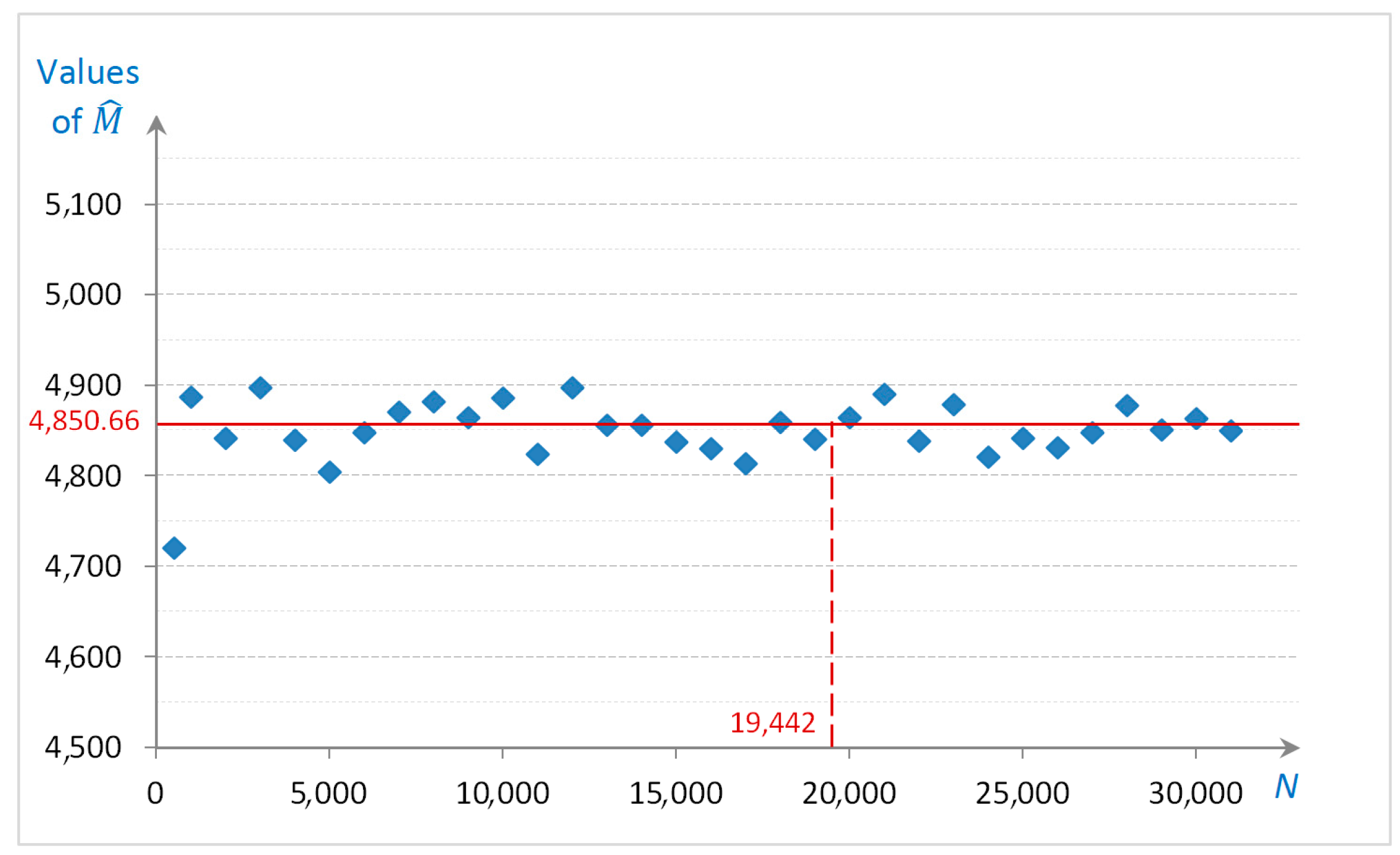
• The input variables identification.
  After consultation with experts from the Maritime Search and Rescue Service, Gdynia, Poland, selected key variables were assumed that can affect the outcome of the simulation: fixed experiment time (affecting the number of simulation iterations), initial probabilities (assumed), probabilities of transitions between the states (calculated from the historical numbers of transitions) and distribution functions (verified statistically). The experiment time is the same for all program projects and was designated on the basis of the simulation convergence. An exemplary illustration is shown in Figure 3.
  There is only one simplification in the model, i.e., the initial probabilities are assumed in a way in which no initiating events happen at t = 0 (all probabilities are equal to 0 at a starting point). This assumption cannot be changed.

  Table A5. Probabilities of transitions between particular states of IE process, based on [41].

  	j	1	2	3	4	5	6	7	8	9	10	11	12	13	14	15	16
  l
  1		–	0.2460	0.2264	0.0754	0.1644	0.1436	0.1258	0.0184	0	0	0	0	0	0	0	0
  2		0.5461	–	0.2880	0.0069	0.0092	0.0507	0.0922	0	0	0.0046	0.0023	0	0	0	0	0
  3		0.9908	0.0026	–	0	0	0.0053	0	0	0.0013	0	0	0	0	0	0	0
  4		0.7450	0.0201	0.0872	–	0	0.0604	0.0873	0	0	0	0	0	0	0	0	0
  5		0.7692	0	0	0	–	0	0	0	0.0659	0.1429	0	0.0037	0	0	0	0.0183
  6		0.4488	0.0989	0.3110	0.0777	0	–	0	0	0	0.0141	0.0495	0	0	0	0	0
  7		0.4115	0	0.5423	0.0038	0	0	–	0.0116	0	0	0.0116	0	0.0192	0	0	0
  8		0.8750	0	0	0	0	0	0	–	0	0	0	0	0.1250	0	0	0
  9		1	0	0	0	0	0	0	0	–	0	0	0	0	0	0	0
  10		0.5790	0	0	0	0	0.3947	0	0	0	–	0	0	0	0.0263	0	0
  11		4444	0	5556	0	0	0	0	0	0	0	–	0	0	0	0	0
  12		1	0	0	0	0	0	0	0	0	0	0	–	0	0	0	0
  13		0.4445	0	0.3333	0	0	0	0	0	0	0	0	0	–	0	0.2222	0
  14		1	0	0	0	0	0	0	0	0	0	0	0	0	–	0	0
  15		0	0	1	0	0	0	0	0	0	0	0	0	0	0	–	0
  16		0.4000	0	0.4000	0	0	0	0.2000	0	0	0	0	0	0	0	0	–

  in Appendix C determines the probabilities of transitions. These input parameters should be randomly sampled from the same matrix that was used to generate the original input parameters, as they are calculated from the historical data. Moreover, the hypotheses on the distribution functions of the realizations of the conditional sojourn times were verified on the basis of the sufficiently large number of realizations, and the empirical distribution functions were determined for numbers of realizations less than 30. This assumption is necessary from the statistical point of view.

• The ranges for input variables statement.
  The generating functions for input parameters remain the same for the input variables and, for this simulation method, they sufficiently reflect the expected variability of the real-world situation being modeled.

• The simulation run.
  The Monte Carlo simulation is run 30 times, each time using a different set of randomly sampled input variables, for a large number of iterations in order to ensure that the results are statistically significant. The simulation time is equal to 25 years and, therefore, the number of iterations is different for each simulation run, depending on the sojourn times.

• The results analysis.
  The statistical measures of interest for the outputs, such as the means and standard deviations, are calculated. These measures can provide an overall understanding of the behavior of the output variables.

• Additional analysis.
  The relationships between the input and output variables have been sufficiently investigated and no further investigation is needed.

• The model adjustments.
  The model can be adjusted using the results of the sensitivity analysis. However, it is also possible to evaluate the significance of the remaining two (simulating successively 35 and then 34 projects). That is why, it is still possible to analyse the sensitivity of the overall output globally to variations in each sub-program.

3.3.3. Limitations and Weaknesses of the Monte Carlo Method

The model used based on the Monte Carlo simulation method, like any other simulation technique, has some limitations and weaknesses. Here are some of them:

• Accuracy depends on the quality of the model: the accuracy of the results obtained depends on the quality of the model used to represent the problem regarding ship accident consequences being analyzed. If the model is oversimplified or does not capture all the important features, the results may not be accurate. Mostly, the accuracy of the model is limited by the accuracy of the input data used. Inaccurate or incomplete data can lead to inaccurate results.
• Computationally intensive: Monte Carlo simulations can be computationally intensive and require a large number of random samples to obtain accurate results. This is a limitation when dealing with a complex problem that requires a significant amount of computational resources. It can lead to long simulation times and high computing costs.
• Uncertainty: simulation-based models are inherently probabilistic, meaning that there is always a degree of uncertainty in the results. This uncertainty can be difficult to quantify and communicate to stakeholders.
• Difficulty in modelling human factors: the method is less effective at modelling the impact of human factors, such as operator error, which can play a significant role in the occurrence and severity of accidents.
• Convergence issues: the convergence of a Monte Carlo simulation can be slow, especially when dealing with systems that exhibit rare events. This can make it difficult to obtain accurate results in a reasonable amount of time. The model is less effective for dealing with rare events, such as major chemical spills or catastrophic accidents, when the degradation effects listed in Table 2 reach high levels of their parameters, or accidents lead to the release of less frequently transported substances, especially those other than oil, due to the low probability of these events occurring (see results given in Section 3.5).
• Requires distributional assumptions: Monte Carlo simulations rely on the assumption that the input variables have statistically verified distributions. This can be a limitation when dealing with a problem in which distribution functions do not fit to any of the known functions.

Despite these limitations, the approach used in the paper remains a powerful tool for modelling and simulating complex problems when requiring expertise in statistical methods and modelling techniques. It is important to be aware of its limitations and weaknesses in order to use it effectively and accurately.

3.3.4. Additional Limitations of the Model

The approach to shipping accidents and chemical release consequences’ assessment involves considering the uncertainties associated with the potential impacts of shipping accidents on the environment and human health. Uncertainty refers to the lack of knowledge or information about the value of a parameter. Some of the values used in Table A5,

Table A6. Probabilities of transitions between particular states of ET process, based on [41].

Subarea	Probabilities of Transitions between Particular States
air	$p_{(1/2)}^{1 27}=p_{(1/2)}^{7 1}=1,$  $p_{(1/2)}^{27 1}=0.977$$, p_{(1/2)}^{27 7}=0.023$; $p_{(1/3)}^{1 23}=0.023,$  $p_{(1/3)}^{1 27}=0.931,$  $p_{(1/3)}^{1 30}=0.046,$  $p_{(1/3)}^{23 1}=p_{(1/3)}^{27 1}=p_{(1/3)}^{30 1}=1$; $p_{(1/4)}^{1 13}=p_{(1/4)}^{1 35}=0.055$  $p_{(1/4)}^{1 27}=0.890,$  $p_{(1/4)}^{5 1}=p_{(1/4)}^{13 1}=p_{(1/4)}^{27 1}=p_{(1/4)}^{35 5}=$1; $p_{(1/5)}^{1 3}=p_{(1/5)}^{1 34}=0.1,$  $p_{(1/5)}^{1 4}=0.3,$  $p_{(1/5)}^{1 27}=0.5,$  $p_{(1/5)}^{3 17}=p_{(1/5)}^{4 1}=p_{(1/5)}^{7 1}=p_{(1/5)}^{17 7}=p_{(1/5)}^{27 1}=p_{(1/5)}^{34 4}=1$; $p_{(1/6)}^{1 27}=p_{(1/6)}^{27 1}=1$; $p_{(1/7)}^{1 27}=0.875$$, p_{(1/7)}^{1 30}=0.125$$, p_{(1/7)}^{27 1}=p_{(1/7)}^{30 1}=1$; $p_{(1/8)}^{1 3}=p_{(1/8)}^{17}=p_{(1/8)}^{1 8}=0.059$$, p_{(1/8)}^{1 6}=0.176$$, p_{(1/8)}^{1 27}=0.647$, $p_{(1/8)}^{3 1}=p_{(1/8)}^{6 1}=p_{(1/8)}^{7 21}=p_{(1/8)}^{8 1}=p_{(1/8)}^{21 1}=p_{(1/8)}^{27 1}=1;$
water surface	$p_{(2/2)}^{1 33}=p_{(2/2)}^{2 1}=1,$  $p_{(2/2)}^{33 1}=0.977$$, p_{(2/2)}^{33 7}=0.023$; $p_{(2/3)}^{1 17}=0.067$$, p_{(2/3)}^{1 18}=0.022$$, p_{(2/3)}^{1 33}=0.911$$, p_{(2/3)}^{17 1}=p_{(2/3)}^{18 1}=p_{(2/3)}^{33 1}=1$; $p_{(2/4)}^{1 33}=p_{(2/4)}^{33 1}=1$; $p_{(2/5)}^{1 33}=p_{(2/5)}^{33 1}=1$; $p_{(2/6)}^{1 33}=p_{(2/6)}^{33 1}=1$; $p_{(2/7)}^{1 17}=0.125$$, p_{(2/7)}^{1 33}=0.875$$, p_{(2/7)}^{17 1}=p_{(2/7)}^{33 1}=1$; $p_{(2/8)}^{1 2}=p_{(2/8)}^{1 4}=p_{(2/8)}^{1 5}=0.071$$, p_{(2/8)}^{1 33}=0.787$$, p_{(2/8)}^{2 1}=p_{(2/8)}^{4 1}=p_{(2/8)}^{5 1}=p_{(2/8)}^{33 1}=1;$
water column	$p_{(3/2)}^{1 24}=p_{(3/2)}^{2 1}=1,$  $p_{(3/2)}^{24 1}=0.977$$, p_{(3/2)}^{24 2}=0.023$; $p_{(3/3)}^{1 14}=0.067$$, p_{(3/3)}^{1 15}=0.022$$, p_{(3/3)}^{1 24}=0.911$$, p_{(3/3)}^{14 1}=p_{(3/3)}^{15 1}=p_{(3/3)}^{24 1}=1$; $p_{(3/4)}^{1 24}=p_{(3/4)}^{24 1}=1$; $p_{(3/5)}^{1 24}=p_{(3/5)}^{24 1}=1$; $p_{(3/6)}^{1 24}=p_{(3/6)}^{24 1}=1$; $p_{(3/7)}^{1 14}=0.125$$, p_{(3/7)}^{1 24}=0.875$$, p_{(3/7)}^{14 1}=p_{(3/7)}^{24 1}=1$; $p_{(3/8)}^{1 2}=p_{(3/8)}^{1 3}=p_{(3/8)}^{1 4}=0.071$$, p_{(3/8)}^{1 24}=0.787$$, p_{(3/8)}^{2 1}=p_{(3/8)}^{3 1}=p_{(3/8)}^{4 1}=p_{(3/8)}^{24 1}=1;$
sea floor	$p_{(4/2)}^{1 2}=0.046,$  $p_{(4/2)}^{1 24}=0.954$$, p_{(4/2)}^{2 1}=p_{(4/2)}^{24 1}=1$; $p_{(4/3)}^{1 14}=0.136,$  $p_{(4/3)}^{1 15}=0.046$$, p_{(4/3)}^{1 24}=0.818$$, p_{(4/3)}^{14 1}={p_{(4/3)}^{15 1}=p}_{(4/3)}^{24 1}=1$; $p_{(4/4)}^{1 24}=p_{(4/4)}^{24 1}=1$; $p_{(4/5)}^{1 24}=p_{(4/5)}^{24 1}=1$; $p_{(4/6)}^{1 24}=p_{(4/6)}^{24 1}=1$; $p_{(4/7)}^{1 14}=0.2$$, p_{(4/7)}^{1 24}=0.8$$, p_{(4/7)}^{14 1}=p_{(4/7)}^{24 1}=1$; $p_{(4/8)}^{1 2}=p_{(4/8)}^{1 4}=0.2$$, p_{(4/8)}^{1 24}=0.6$$, p_{(4/8)}^{2 1}=p_{(4/8)}^{4 1}=p_{(4/8)}^{24 1}=1;$
coast	$p_{(5/2)}^{1 24}=p_{(5/2)}^{24 1}=1$; $p_{(5/3)}^{1 15}=0.062$$, p_{(5/3)}^{1 24}=0.938$$, {p_{(5/3)}^{15 1}=p}_{(5/3)}^{24 1}=1$; $p_{(5/4)}^{1 24}=p_{(5/4)}^{24 1}=1$; $p_{(5/5)}^{1 24}=p_{(5/5)}^{24 1}=1$; $p_{(5/6)}^{1 24}=p_{(5/6)}^{24 1}=1$; $p_{(5/7)}^{1 24}=p_{(5/7)}^{24 1}=1$; $p_{(5/8)}^{1 24}=p_{(5/8)}^{24 1}=1$.

and

Table A7. Probabilities of transitions between particular states of ED process, based on [41].

Subarea	Probabilities of Transitions between Particular States
air	$q_{(1/3)}^{1 28}=q_{(1/3)}^{6 1}=q_{(1/3)}^{22 6}=q_{(1/3)}^{25 22}=q_{(1/3)}^{28 25}=1$; $q_{(1/4)}^{1 27}=0.75$$, q_{(1/4)}^{1 30}=0.25$$, q_{(1/4)}^{20 1}=q_{(1/4)}^{21 1}=q_{(1/4)}^{24 21}=q_{(1/4)}^{27 24}=q_{(1/4)}^{29 20}=q_{(1/4)}^{30 29}=1$; ${q_{(1/5)}^{1 26}=q}_{(1/5)}^{20 1}=q_{(1/5)}^{23 20}=q_{(1/5)}^{26 23}=1$; $q_{(1/6)}^{1 2}=0.667$$, q_{(1/6)}^{1 19}=0.333$$, q_{(1/6)}^{2 1}=q_{(1/6)}^{17 1}=q_{(1/6)}^{18 17}=q_{(1/6)}^{19 18}=1$; $q_{(1/7)}^{1 2}=q_{(1/7)}^{1 10}=0.5$$, q_{(1/7)}^{2 1}=q_{(1/7)}^{6 1}=q_{(1/7)}^{8 6}=q_{(1/7)}^{10 8}=1$; $q_{(1/8)}^{1 15}=q_{(1/8)}^{13 1}=q_{(1/8)}^{14 13}=q_{(1/8)}^{15 14}=1$; $q_{(1/13)}^{1 6}=q_{(1/13)}^{6 1}=1$; $q_{(1/17)}^{1 28}=q_{(1/17)}^{6 1}=q_{(1/17)}^{22 6}=q_{(1/17)}^{25 22}=q_{(1/17)}^{28 25}=1$; $q_{(1/21)}^{1 20}=q_{(1/21)}^{20 1}=1$; $q_{(1/23)}^{1 2}=q_{(1/23)}^{2 1}=1$; $q_{(1/27)}^{1 6}=q_{(1/27)}^{6 1}=1$; $q_{(1/30)}^{1 11}=q_{(1/30)}^{11 1}=1$; $q_{(1/35)}^{1 26}=q_{(1/35)}^{20 1}=q_{(1/35)}^{23 20}=q_{(1/35)}^{26 23}=1$;
water surface	$q_{(2/1)}^{1 5}=q_{(2/1)}^{5 1}=1$; $q_{(2/2)}^{1 2}=q_{(2/2)}^{2 1}=1$; $q_{(2/4)}^{1 2}=q_{(2/4)}^{2 1}=1$; $q_{(2/5)}^{1 18}=q_{(2/5)}^{13 1}=q_{(2/5)}^{14 13}=q_{(2/5)}^{18 14}=1$; $q_{(2/17)}^{1 25}=q_{(2/17)}^{1 27}=0.5$$, q_{(2/17)}^{12 1}=q_{(2/17)}^{16 12}=q_{(2/17)}^{21 16}=q_{(2/17)}^{25 21}=q_{(2/17)}^{27 25}=1$; $q_{(2/18)}^{1 11}=q_{(2/18)}^{6 1}=q_{(2/18)}^{9 6}=q_{(2/18)}^{11 9}=1$; $q_{(2/33)}^{1 6}=0.480$$, q_{(2/33)}^{1 9}=q_{(2/33)}^{1 11}=0.256$$, q_{(2/33)}^{1 23}=0.008$, $q_{(2/33)}^{2 1}=q_{(2/33)}^{6 1}=q_{(2/33)}^{9 6}=q_{(2/33)}^{11 9}=q_{(2/33)}^{12 2}=q_{(2/33)}^{15 12}=q_{(2/33)}^{20 15}=q_{(2/33)}^{22 20}=q_{(2/33)}^{23 22}=1$
water column	$q_{(3/2)}^{1 2}=q_{(3/2)}^{2 1}=1$; $q_{(3/3)}^{1 2}=q_{(3/3)}^{2 1}=1$; $q_{(3/4)}^{1 18}=q_{(3/4)}^{13 1}=q_{(3/4)}^{14 13}=q_{(3/4)}^{18 14}=1$; $q_{(3/14)}^{1 25}=q_{(3/14)}^{1 27}=0.5$$, q_{(3/14)}^{12 1}=q_{(3/14)}^{16 12}=q_{(3/14)}^{21 16}=q_{(3/14)}^{25 21}=q_{(3/14)}^{27 25}=1$; $q_{(3/15)}^{1 11}=q_{(3/15)}^{6 1}=q_{(3/15)}^{9 6}=q_{(3/15)}^{11 9}=1$; $q_{(3/24)}^{1 6}=0.648$$, q_{(3/24)}^{1 9}=0.296$$, q_{(3/24)}^{1 11}=0.048$$, q_{(3/24)}^{1 23}=0.008$$, q_{(3/24)}^{6 1}=0.961$$, q_{(3/24)}^{6 9}=0.039$, $q_{(3/24)}^{9 6}=0.857$$, q_{(3/24)}^{9 11}=0.143$$, q_{(3/24)}^{2 1}=q_{(3/24)}^{11 9}=q_{(3/24)}^{12 2}=q_{(3/24)}^{15 12}=q_{(3/24)}^{20 15}=q_{(3/24)}^{22 20}=q_{(3/24)}^{23 22}=1$
sea floor	$q_{(4/1)}^{1 2}=q_{(4/1)}^{2 1}=1$; $q_{(4/4)}^{1 18}=q_{(4/4)}^{13 1}=q_{(4/4)}^{14 13}=q_{(4/4)}^{18 14}=1$; $q_{(4/14)}^{1 28}=q_{(4/14)}^{1 30}=0.5$$, q_{(4/14)}^{12 1}=q_{(4/14)}^{16 12}=q_{(4/14)}^{21 16}=q_{(4/14)}^{28 21}=q_{(4/14)}^{30 28}=1$; $q_{(4/15)}^{1 11}=q_{(4/15)}^{6 1}=q_{(4/15)}^{9 6}=q_{(4/15)}^{11 9}=1$; $q_{(4/24)}^{1 6}=0.912,$$q_{(4/24)}^{1 9}=0.070,$$q_{(4/24)}^{1 11}=0.018$$, q_{(4/24)}^{6 1}=0.600$$, q_{(4/24)}^{6 9}=0.390$$, q_{(4/24)}^{6 24}=0.010$, $q_{(4/24)}^{9 6}=0.610$$, q_{(4/24)}^{9 11}=0.280$$, q_{(4/24)}^{9 25}=0.110$$, q_{(4/24)}^{11 9}=0.294$$, q_{(4/24)}^{11 26}=0.706$$, q_{(4/24)}^{24 6}=1$, $q_{(4/24)}^{25 6}=0.857$$, q_{(4/24)}^{25 24}=0.143$$, q_{(4/24)}^{26 9}=0.917$$, q_{(4/24)}^{26 25}=0.083$
coast	$q_{(5/1)}^{1 2}=q_{(5/1)}^{5 1}=1$; $q_{(5/15)}^{1 11}=q_{(5/15)}^{6 1}=q_{(5/15)}^{9 6}=q_{(5/15)}^{11 9}=1$; $q_{(5/24)}^{1 6}=0.745,$$q_{(5/24)}^{1 9}=0.177,$$q_{(5/24)}^{1 11}=0.078$$, q_{(5/24)}^{6 1}=0.699$$, q_{(5/24)}^{6 9}=0.301$$, q_{(5/24)}^{9 6}=0.761$, $q_{(5/24)}^{9 11}=0.239$$, q_{(5/24)}^{11 9}=1$

(Appendix C) are not known (there is no empirical data) and are assumed to be 0, or there is little data (the empirical distributions were assumed for the sets containing less than 30 elements). The uncertainty assessment for these parameters could be enhanced with the availability of additional data or information. Uncertainties also arise due to a lack of knowledge about the specific details of the accident scenario, as well as natural variability in environmental conditions and human responses. The potential impacts of the accidents were estimated with a range of probabilities. This approach can allow assessment of the risks associated with different accident scenarios and evaluation of the effectiveness of different response and mitigation strategies.

3.3.5. Justification of the Programming Language Used

There are several reasons why C# is a good choice for a simulation-based model. It is a powerful and flexible language that is well-suited to simulation development. First of all, it is an object-oriented programming language, which means that it allows for the creation of complex, modular simulations with reusable code. Moreover, the language is cross-platform, which means that it was used to develop simulations across different operating systems, including Windows and macOS, and can also be used on Linux. The language is designed to work well with other Microsoft tools, such as Visual Studio, which provide a comprehensive development environment for modelling. C# language comes with a large standard library, providing a range of pre-built functionality which was used to speed up the Monte Carlo simulation. This reach framework offers much control over memory management and garbage collection, which automatically frees up memory when it is no longer needed. Namely, it has automatic memory management with no need to manage memory manually, making it easier to write and maintain the code and reducing the risk of memory leaks and crashes. It is a compiled language, which means that it is generally faster than interpreted languages, such as Python. This makes it a good choice for simulations that require high performance.

C and C++ are also popular languages for simulation, but they have different strengths and weaknesses compared to C#. C is a low-level language that is often used in systems programming and for developing operating systems. It is fast and efficient, but it requires more manual memory management than higher-level languages like C#. C++ is an object-oriented extension of C that is often used in developing applications and games, but can be more difficult to learn and use.

3.4. Prediction of Shipping Accident Consequences

The results obtained in Section 3.2 are essential to predict characteristics of the particular processes: the IE process, the ET process and the ED process. In this way, the approximate limit values of transient probabilities at particular states of these processes are predicted and the results are presented in Section 3.4.1–Section 3.4.3. The following results are obtained for 25 years. Moreover, using these results, the approximate mean values of sojourn total time of these processes at their particular states during the fixed time (e.g., 1 year) can be obtained.

The mean values presented in Table 3, Table 4, Table 5 and Table 6 are calculated using the very detailed obtained limit transient probabilities, taken with a precision of 15–17 decimal places (double floating-point type). To show the values in an accessible way, they are approximated to five decimal places in this article.

3.4.1. Prediction of the IE Process

The approximate limit transient probabilities and the approximate mean values of the sojourn total times during the fixed time of 1 year = 8760 h at the particular states are given in Table 3.

The results given in Table 3 allow a statement that, fortunately, no IE dangerous to the environment surrounding the accident area takes place after a ship accident, as the state $e^1$ reaches the greatest probability $p^1=$ 0.99965 (the meaning of state $e^1$ is explained in Section 3.1.1, as well as in Table A2 of Appendix B). Consequently, the mean sojourn total time for the state $e^1$ also reaches the greatest value (${\widehat{M}}^1=$ 8756.9 hr/year).

As we can see in Table 3, not all the states occurred, or occurred only with a very small probability in a given simulation. Therefore, an additional simulation is carried out for a longer duration of the experiment to increase the number of iterations, and thus the realizations of the total numbers of process transitions. The results are presented in Table 4 (increasing the time to make the majority of the realizations statistically significant).

If the obtained characteristics are compared with those obtained for 1 year, it can be noticed that, apart from the values obtained in the first simulation, all other values are close to zero.

3.4.2. Prediction of the Conditional ET Process

The approximate limit of transient probabilities and the approximate mean values of the sojourn total times during the fixed time of 1 year = 8760 h at the particular states are given in Table 5.

The results given in Table 5 allow a statement that the most likely threats as a result of sea accident are typically oil spills and connected with the presence in the accident area of moderate toxic and moderate bio-accumulative substances causing additional long-term effects, as the states $s_{\left(1\right)}^{27}$, $s_{\left(2\right)}^{33}$, $s_{\left(3\right)}^{24}$, $s_{\left(4\right)}^{24}$ and $s_{\left(5\right)}^{24}$ reach the greatest probability (the meaning of these states is explained in Section 3.1.2 and in Table A3 of Appendix B). Consequently, the mean sojourn total times for these states also reach the greatest value.

3.4.3. Prediction of the Conditional ED Process

The approximate limit of transient probabilities and the approximate mean values of sojourn total times during the fixed time 1 year = 8760 h at the particular states are given in Table 6.

The results given in Table 6 allow a statement that the most likely degradation effects as a result of sea accident are typically oil spills and connected with aesthetic nuisance and pollution of air and water. as the states e.g., $r^2$ and $r^6$ in particular environmental sub-areas reach the greatest probability (the meaning of these states is explained in Section 3.1.3 and in Table A4 of Appendix B). Consequently, the mean sojourn total times for these states also reach the greatest value.

3.5. Joint IE Process, ET Process and ED Process—Superposition

The IE, ET and ED processes are predicted and the characteristics, such as approximate limit values of transient probabilities and approximate mean values of sojourn total time, of these particular processes at their states are obtained in Section 3.4. Then these results are used in superposition for these three particular processes to find the unconditional limit transient probabilities of the joint processes, i.e., the unconditional ED process, applying Formula (2). The results are as follows:

$$\begin{array}{c}{q}_{\left(1\right)}^1= 0.99966545925, q_{\left(1\right)}^2= 0.00000059326, q_{\left(1\right)}^6=0.00033263931,\\ q_{\left(1\right)}^8= 0.00000000001, q_{\left(1\right)}^{10}= 0.00000000003, q_{\left(1\right)}^{11}= 0.00000130814,\\ q_{\left(1\right)}^{13}=q_{\left(1\right)}^{14}=q_{\left(1\right)}^{15}=q_{\left(1\right)}^{17}=q_{\left(1\right)}^{18}=q_{\left(1\right)}^{19}=q_{\left(1\right)}^{20}=q_{\left(1\right)}^{22}=q_{\left(1\right)}^{23}=q_{\left(1\right)}^{24}{=q}_{\left(1\right)}^{25}=q_{\left(1\right)}^{26}\\ =q_{\left(1\right)}^{27}=q_{\left(1\right)}^{28}=q_{\left(1\right)}^{29}=q_{\left(1\right)}^{30}\cong 0;\\ \\ q_{\left(2\right)}^1= 0.99964910673, q_{\left(2\right)}^2= 0.00002785620, q_{\left(2\right)}^5= 0.00000485401,\\ q_{\left(2\right)}^6= 0.00024367125, q_{\left(2\right)}^9= 0.00003133615, q_{\left(2\right)}^{11}= 0.00002267715,\\ q_{\left(2\right)}^{12}= 0.00000799881, q_{\left(2\right)}^{13}=q_{\left(2\right)}^{14}\cong 0, q_{\left(2\right)}^{15}= 0.00000081432,\\ q_{\left(2\right)}^{16}= 0.00000539187, q_{\left(2\right)}^{18}\cong 0, q_{\left(2\right)}^{20}= 0.00000114005,\\ q_{\left(2\right)}^{21}= 0.00000385746, q_{\left(2\right)}^{22}= 0.00000016286, q_{\left(2\right)}^{23}= 0.00000016286,\\ q_{\left(2\right)}^{25}= 0.00000061269, q_{\left(2\right)}^{27}= 0.00000035759;\\ \\ q_{\left(3\right)}^1= 0.99965321112, q_{\left(3\right)}^2= 0.00002309595, q_{\left(3\right)}^6= 0.00023666753,\\ q_{\left(3\right)}^9= 0.00006153819, q_{\left(3\right)}^{11}= 0.00000891299, q_{\left(3\right)}^{12}= 0.00000654619,\\ q_{\left(3\right)}^{13}=q_{\left(3\right)}^{14}\cong 0, q_{\left(3\right)}^{15}= 0.00000067514, q_{\left(3\right)}^{16}= 0.00000427886,\\ q_{\left(3\right)}^{18}\cong 0, q_{\left(3\right)}^{20}= 0.00000094519, q_{\left(3\right)}^{21}= 0.00000306513,\\ q_{\left(3\right)}^{22}= 0.00000013503, q_{\left(3\right)}^{23}= 0.00000013503, q_{\left(3\right)}^{25}= 0.00000051573,\\ q_{\left(3\right)}^{27}= 0.00000027792;\\ \\ q_{\left(4\right)}^1= 0.99968141400, q_{\left(4\right)}^2= 0.00000000762, q_{\left(4\right)}^6= 0.00004440480,\\ q_{\left(4\right)}^9= 0.00022776002, q_{\left(4\right)}^{11}= 0.00003047766, q_{\left(4\right)}^{12}= 0.00000606086,\\ q_{\left(4\right)}^{13}=q_{\left(4\right)}^{14}\cong 0, q_{\left(4\right)}^{16}= 0.00000486991,\\ q_{\left(4\right)}^{18}\cong 0, q_{\left(4\right)}^{21}= 0.00000343185, q_{\left(4\right)}^{24}= 0.00000007136,\\ q_{\left(4\right)}^{25}= 0.00000024837, q_{\left(4\right)}^{26}= 0.00000034305, q_{\left(4\right)}^{28}= 0.00000058641,\\ q_{\left(4\right)}^{30}= 0.00000032410;\\ \\ q_{\left(5\right)}^1= 0.99965166582, q_{\left(5\right)}^5= 0.00000377608, q_{\left(5\right)}^6= 0.00019470512,\\ q_{\left(5\right)}^9= 0.00006989055, q_{\left(5\right)}^{11}= 0.00007996243.\end{array}$$

The above results are essential as they can be used to obtain the mean values of sojourn total times for the unconditional ED process, during the fixed time of 1 year = 8760 h, according to the Formula (11), for $p^i:=q_{\left(k\right)}^i$. The results are as follows (${\widehat{M}}_{\left(k\right)}^i$ equal to 0 are omitted):

$$\begin{array}{c}{\widehat{M}}_{\left(1\right)}^1= 8757.06942, {\widehat{M}}_{\left(1\right)}^2= 0.00520, {\widehat{M}}_{\left(1\right)}^6= 2.91392, {\widehat{M}}_{\left(1\right)}^{11}= 0.01146;\\ \\ {\widehat{M}}_{\left(2\right)}^1= 8756.92618, {\widehat{M}}_{\left(2\right)}^2= 0.24402, {\widehat{M}}_{\left(2\right)}^5= 0.04252, {\widehat{M}}_{\left(2\right)}^6= 2.13456,\\ \\ {\widehat{M}}_{\left(2\right)}^9= 0.27450, {\widehat{M}}_{\left(2\right)}^{11}= 0.19865, {\widehat{M}}_{\left(2\right)}^{12}= 0.07007, {\widehat{M}}_{\left(2\right)}^{15}= 0.00713,\\ \\ {\widehat{M}}_{\left(2\right)}^{16}= 0.04723, {\widehat{M}}_{\left(2\right)}^{20}= 0.00999, {\widehat{M}}_{\left(2\right)}^{21}= 0.03379, {\widehat{M}}_{\left(2\right)}^{22}= 0.00143,\\ \\ {\widehat{M}}_{\left(2\right)}^{23}= 0.00143, {\widehat{M}}_{\left(2\right)}^{25}= 0.00537, {\widehat{M}}_{\left(2\right)}^{27}= 0.00313;\\ \\ {\widehat{M}}_{\left(3\right)}^1= 8756.96213, {\widehat{M}}_{\left(3\right)}^2= 0.20232, {\widehat{M}}_{\left(3\right)}^6= 2.07321, {\widehat{M}}_{\left(3\right)}^9= 0.53907,\\ \\ {\widehat{M}}_{\left(3\right)}^{11}= 0.07808, {\widehat{M}}_{\left(3\right)}^{12}= 0.05735, {\widehat{M}}_{\left(3\right)}^{15}= 0.00591, {\widehat{M}}_{\left(3\right)}^{16}= 0.03748,\\ \\ {\widehat{M}}_{\left(3\right)}^{20}= 0.00828, {\widehat{M}}_{\left(3\right)}^{21}= 0.02685, {\widehat{M}}_{\left(3\right)}^{22}= 0.00118, {\widehat{M}}_{\left(3\right)}^{23}= 0.00118,\\ \\ {\widehat{M}}_{\left(3\right)}^{25}= 0.00452, {\widehat{M}}_{\left(3\right)}^{27}= 0.00244;\\ \\ {\widehat{M}}_{\left(4\right)}^1= 8757.20919, {\widehat{M}}_{\left(4\right)}^2= 0.00007, {\widehat{M}}_{\left(4\right)}^6= 0.38899, {\widehat{M}}_{\left(4\right)}^9= 1.99518,\\ \\ {\widehat{M}}_{\left(4\right)}^{11}= 0.26698, {\widehat{M}}_{\left(4\right)}^{12}= 0.05309, {\widehat{M}}_{\left(4\right)}^{16}= 0.04266, {\widehat{M}}_{\left(4\right)}^{21}= 0.03006,\\ \\ {\widehat{M}}_{\left(4\right)}^{24}= 0.00062, {\widehat{M}}_{\left(4\right)}^{25}= 0.00218, {\widehat{M}}_{\left(4\right)}^{26}= 0.00300, {\widehat{M}}_{\left(4\right)}^{28}= 0.00514,\\ \\ {\widehat{M}}_{\left(4\right)}^{30}= 0.00284;\\ \\ {\widehat{M}}_{\left(5\right)}^1= 8756.94859, {\widehat{M}}_{\left(5\right)}^5= 0.03308, {\widehat{M}}_{\left(5\right)}^6= 1.70562, {\widehat{M}}_{\left(5\right)}^9= 0.61224,\\ \\ {\widehat{M}}_{\left(5\right)}^{11}=0.70047.\end{array}$$

4. Discussion

Using the Monte Carlo simulation technique, three considered processes’ (IE, ET and ED) predicted characteristics are obtained for a 25 years period of time for the sea area. Specifically, the limit values of transient probabilities and the mean values of total sojourn times for the fixed time at the fixed states of particular processes are determined in the paper. A study was carried out for different and increasing numbers of simulation iterations $N$, shown in Figure 3. This was done for a randomly selected process (ED) and its sub-area (air): ${\widehat{M}}_{(1/4)}^{27}$. It is clear that the relative errors between the simulation and analytical expected values of the considered unconditional lifetime are decreasing. For example if $N=19442$ the relative error equals

$$RE=\frac{\left|{{\widehat{M}}_{(1/4)}^{27}}_{\mathrm{simulation}}-{{\widehat{M}}_{(1/4)}^{27}}_{\mathrm{analytical}}\right|}{{{\widehat{M}}_{(1/4)}^{27}}_{\mathrm{analytical}}}\cong 0.00121748 \approx 0.12\%.$$

This means that the number of iterations taken into account is reasonable in this case.

The weakness of the simulation-based model used in this paper is that the use of a pseudo-random number generator can result in different sequences of numbers, which can affect the results of the simulation and make it difficult to reproduce the same results. A sequence of numbers generated by a pseudo-random number generator is determined by an initial value, known as the seed value. If the same seed value is set and the same number of random numbers is generated using the same procedure, the same sequence of numbers will be obtained every time. Nevertheless, if the seed value is even slightly altered, a different sequence of numbers will be produced. Hence, while the numbers may seem random, they are actually deterministic and can be predicted based on the seed value and the procedure utilized to generate them. To overcome this difficulty, it is recommended to use multiple random number generators with different seed values and procedures, or to use a method called “quasi-random sampling” which uses a more structured approach to generate samples. On the other hand, C# is a high-level language that offers features such as automatic memory management, a simpler syntax and a rich class library that makes it easier to write code quickly and reliably.

Furthermore, performing a sensitivity analysis on the model helped to identify how sensitive the results are to variations in the input parameters and can provide insights into the robustness of the model. It seemed reasonable to focus on the sub-program for the IE process, because this can have the most significant impact on the results. It is crucial for the assessment of shipping accident consequences and the environmental degradation.

The sensitivity analysis for the first program (process IE) was carried out and the one output parameter (${\widehat{M}}_{\left(1\right)}^1$) of 16 was plotted against the range of values for the input variables (in this case, the states generated and the numbers of simulation iterations were different). Figure 4 can help us visualize how changes in the input variables affect the output variable ${\widehat{M}}_{\left(1\right)}^1$.

Therefore, the model can be adjusted and it is possible to evaluate the significance of the remaining two program projects (simulating successively 35 and then 34 projects for ET and ED). That is why it is still possible to analyse the sensitivity of the overall output globally to variations in each sub-program. The Monte Carlo simulation can be run to obtain the outputs for each set of input values. Based on the sensitivity analysis results, adjustments can be made to the sub-programs to improve their accuracy, or other modifications can be made to improve the overall performance of the program.

The main results of the study are presented in Section 3.4, where the unconditional limit transient probabilities of the previously defined kinds of environmental degradation effects are considered as the consequences of ships’ accidents at seas in the global scale. These consequences and their probabilities are established in regards to five sub-areas of marine environment (air, water surface, water column, sea floor and coast).

The results show that states $r_{\left(1\right)}^1,$ $r_{\left(2\right)}^1,$ $r_{\left(3\right)}^1,$ $r_{\left(4\right)}^1$, and $r_{\left(5\right)}^1$ reach the highest value of transient probabilities, approximately equal to $q_{\left(1\right)}^1=$ $q_{\left(2\right)}^1=$ $q_{\left(3\right)}^1=$ $q_{\left(4\right)}^1=$ $q_{\left(5\right)}^1\cong 0.9997$. This means that the vast majority of accidents cause no degradation effects within all considered sub-areas of the maritime environment (Figure 5, Figure 6, Figure 7, Figure 8 and Figure 9). Disregarding these values, other states of environmental degradation that reach the noticeable values of limit transient probabilities are:

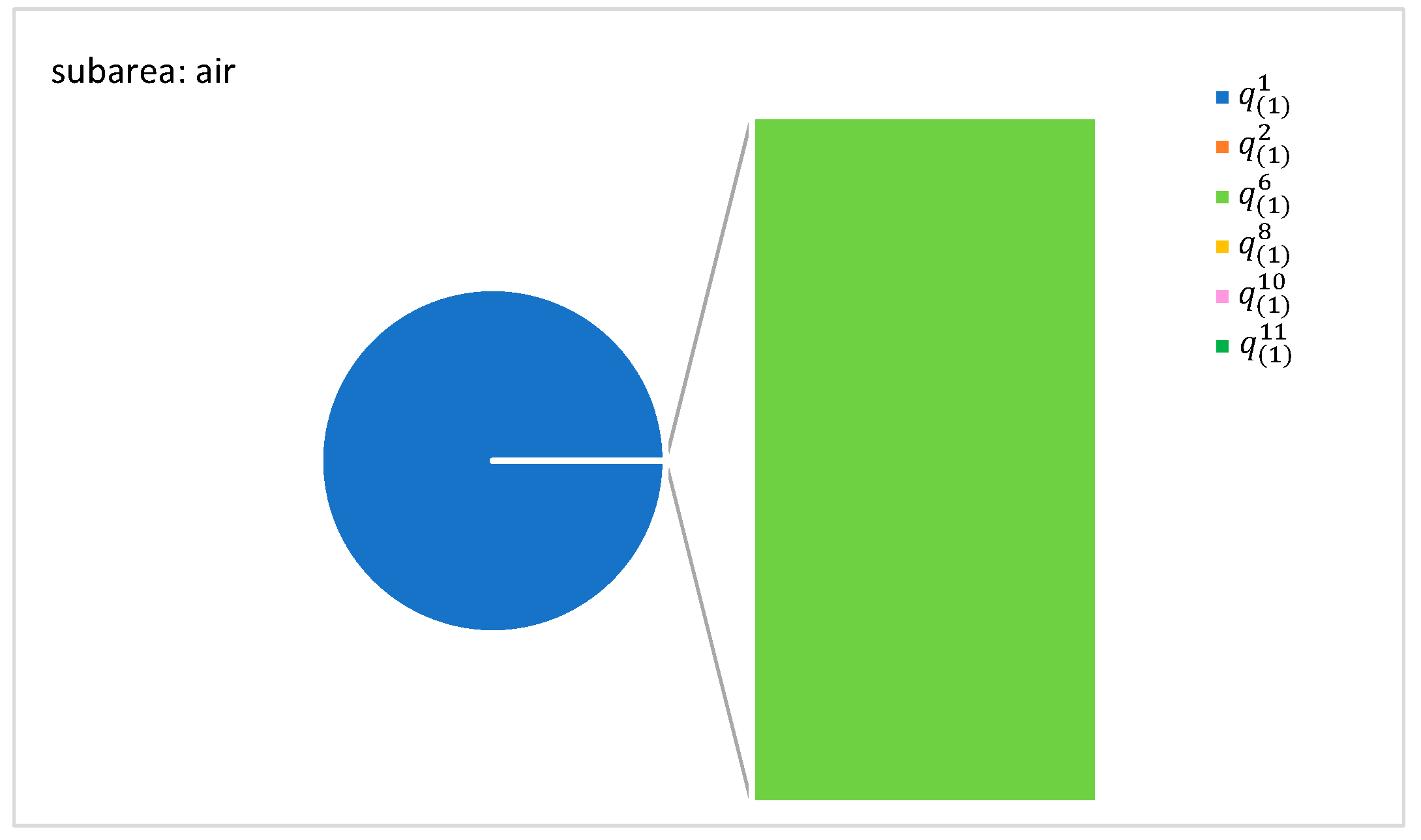
• within the air subarea: $r_{\left(1\right)}^6$ reaches the value of the transient probability equals to $q_{\left(1\right)}^6\cong$ 0.00033, which means that this state lasts ${\widehat{M}}_{\left(1\right)}^6\cong$ 2.9 h per a year (Figure 5);
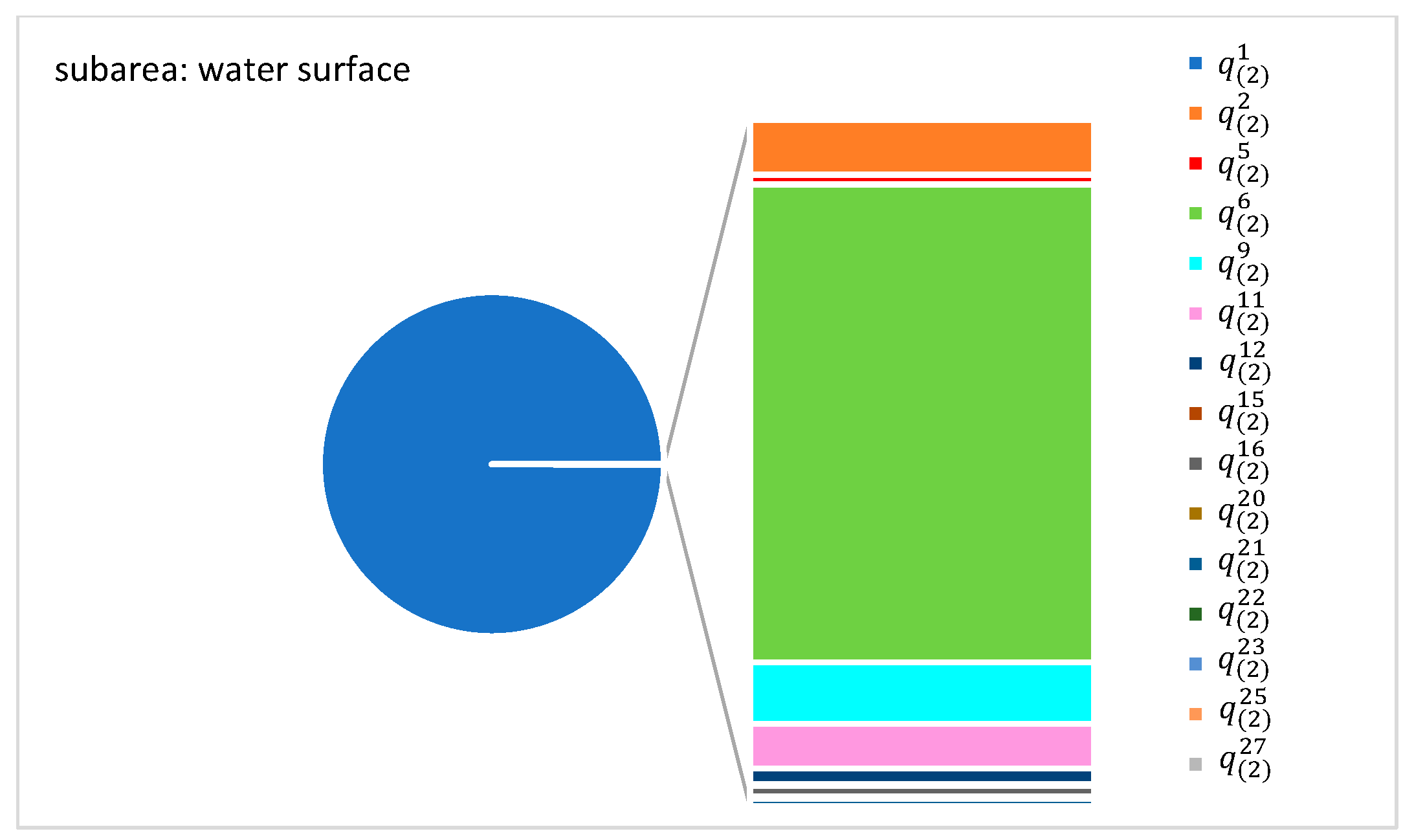
• within the water surface subarea: $r_{\left(2\right)}^6$ reaches the value of the transient probability equals to $q_{\left(2\right)}^6\cong$ 0.00024, which means that this state lasts ${\widehat{M}}_{\left(2\right)}^6\cong$ 2.1 h per a year (Figure 6);
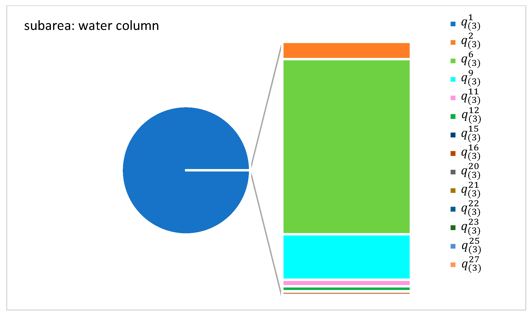
• within the water column subarea: $r_{\left(3\right)}^6$ and $r_{\left(3\right)}^9$ reach the value of the transient probabilities equal to $q_{\left(3\right)}^6\cong$ 0.00024 and $q_{\left(3\right)}^9\cong$ 0.00006 respectively, which means that these states lasts ${\widehat{M}}_{\left(3\right)}^6\cong$ 2.1 and ${\widehat{M}}_{\left(3\right)}^9\cong$ 0.5 h per a year (Figure 7);
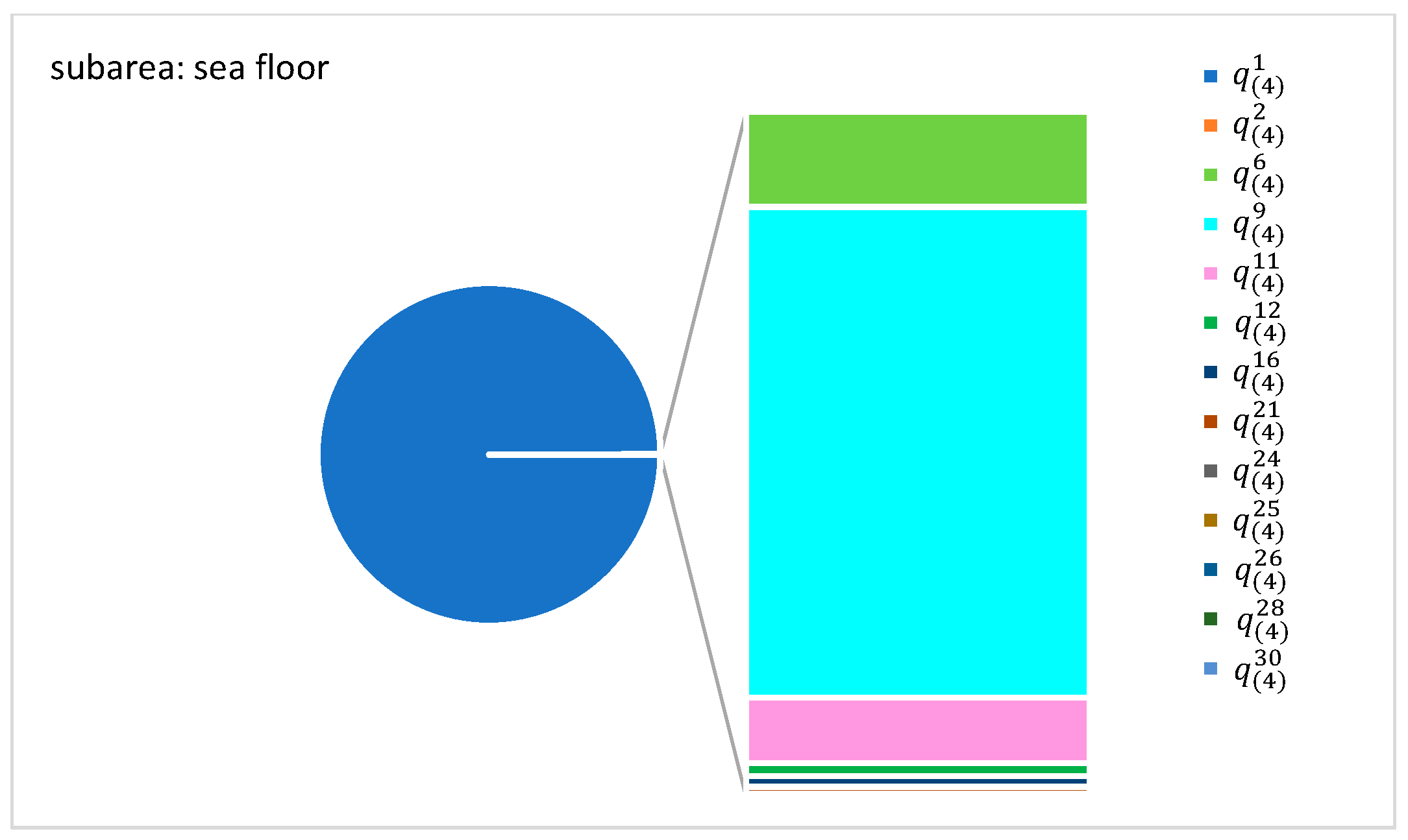
• within the sea floor subarea: $r_{\left(4\right)}^6$ and $r_{\left(4\right)}^9$ reach the value of the transient probabilities equal to $q_{\left(4\right)}^6\cong$ 0.00004 and $q_{\left(4\right)}^9\cong$ 0.00023 respectively, which means that these states last ${\widehat{M}}_{\left(4\right)}^6\cong$ 0.4 and ${\widehat{M}}_{\left(4\right)}^9\cong$ 2.0 h per a year (Figure 8);
• within the coast subarea: $r_{\left(5\right)}^6,$ $r_{\left(5\right)}^9$ and $r_{\left(5\right)}^{11}$ reach the value of the transient probabilities equal to $q_{\left(5\right)}^6=$ 0.00019, $q_{\left(5\right)}^9\cong$ 0.00007 and $q_{\left(5\right)}^{11}\cong$ 0.00008 respectively, which means that these states last ${\widehat{M}}_{\left(5\right)}^6\cong$ 1.7, ${\widehat{M}}_{\left(5\right)}^9\cong$ 0.6 and ${\widehat{M}}_{\left(5\right)}^{11}\cong$ 0.7 h per year (Figure 9).

The states mentioned above are related to the environmental degradation when aesthetic nuisance and pollution are caused by the presence of toxic substances in the ship accident area (see: Table 1 and Table A4 of Appendix B). These results are typical during oil spills and closure of the accidental area is usually not required, or temporarily required for no more than 48 h.

The values of probabilities of other states of ED in particular sub-areas are so insignificant that they are not mentioned above. Consequently, this means that the mean values of sojourn total times of these states equals approximately less than an hour per year.

5. Conclusions

The paper presents an innovative approach to modelling the consequences of shipping accidents and chemical releases in sea waters. The Monte Carlo simulation technique combined with the semi-Markov model is a general technique, but in the paper is applied in different fields, and they have never been used in the form of their superposition and its application in the analysis of maritime transport accident consequences. The superposition of three processes (process of initiating events, process of environmental threats and process of environmental degradation) based on their semi-Markov models is an original approach and there is a genuine need for more exact investigation of accident consequences, which are very complex and require the proposed, practically important tool. The usage of Monte Carlo simulation with a semi-Markov model allows for a probabilistic analysis of the processes involved, which can be useful further for decision-making purposes.

The study and obtained results confirm that oil is the most frequent substance (being both the cargo and the fuel of ships) that causes pollution and has a devastating impact on the marine environment [5,7,57,58]. Oil is toxic to many marine organisms, including fish, mammals, birds and invertebrates. When oil spills occur, it can contaminate the water and the sea floor, causing harm to the ecosystem. Oil spills can also harm habitats such as coral reefs, seagrass beds and wetlands, which provide critical breeding and feeding grounds for many marine species. As well as these environmental consequences, oil spills can cause economic and social consequences [59,60,61]. The main economic consequences are to the fishing and tourism industries. Fishing is often suspended after an oil spill due to concerns about the safety of seafood, which can lead to economic losses for fishermen and seafood processors. Similarly, tourism can be impacted by the presence of oil on beaches and in the water, leading to canceled trips and lost revenue for businesses that depend on tourism. This is connected with social consequences, particularly for communities that rely on fishing or tourism for their livelihoods. These communities may suffer economic hardship and stress, and oil spills can also impact their health and wellbeing. Additionally, oil spills can cause conflict between different groups, such as fishermen, oil companies and government agencies. Thus, oil spills at sea can have significant and long-lasting consequences for the environment, economy and society, underscoring the importance of preventing and responding to them. Therefore both proactive and reactive strategies play essential roles in the emergency response process to an oil spill [62,63]. The proactive strategy focuses on preventing an oil spill from happening in the first place. This includes measures such as regular maintenance of tankers to prevent leaks, implementing safety procedures and protocols, and conducting regular safety drills to prepare for emergencies. In addition, there are regulations and standards in place to ensure that ships operate in a safe and responsible manner to minimize the risk of oil spills. This study points out the type of common pollutant that oil is, which the maritime salvage companies will have to combat and remove from the ecosystem. This knowledge, as an element of proactive strategy in the prevention of environmental degradation, permits preparation for emergency response process in advance. The reactive strategy focuses on responding to an oil spill once it has occurred. This includes measures such as deploying oil spill response teams, containing and recovering spilled oil, and cleaning up affected areas. Reactive measures are typically activated once an oil spill is detected, and they aim to minimize the impact of the spill on the environment, economy, and society. Therefore, an important role in reactive strategy is modelling, prediction and determining the shape and direction of oil spread under variable hydro-meteorological conditions [64,65,66]. Both proactive and reactive strategies are critical components of the emergency response process. While proactive strategy aims to prevent oil spills, reactive strategy provides a rapid and effective response to minimize the damage caused by the spills that do occur. By combining both strategies, we can reduce the risk of oil spills and minimize their impact when they do occur.

This study also has some limitations. Apart from those mentioned in Section 3.3.3 and Section 3.3.4, due to the fact that the results are evaluated on the basis of real statistical data coming from maritime accidents over an 11-year period as the experimental timescale for this research, their values may change and become more precise if the duration of the experiment is longer. Therefore, future studies with a larger sample of statistical data are recommended. Moreover, as to the limitations of this study, this research concentrates on shipping accidents’ consequences without considering impacts of any environmental factors, e.g., weather influence. Yet, despite these limitations, the current findings may constitute a basis for discussion and a starting point that will stimulate further extended research.

The above mentioned limitations set the direction for future studies. It could be highly interesting in future research to extend the model of shipping accident and chemical release consequences by adding weather impact. The first attempts have been made in [41,67], where only the influence of sea wave height, wind speed and direction were taken into consideration. Moreover, other parameters such as the temperature of water and air and the salinity of sea water, which are crucially significant to the range of environmental degradations caused by chemical releases, should be investigated. Moreover, optimized modeling techniques could be used to improve the simulation results, adjusting them more to reality.

An explanation and a summary of the key findings of the study, highlighting the most important results and insights, are illustrated in Figure 10.

References

- National Research Council. Vessel Navigation and Traffic Services for Safe and Efficient Ports and Waterways: Interim Report; The National Academies Press: Washington, DC, USA, 1996. [Google Scholar] [CrossRef]
- Bekir, E. Introduction to Modern Navigation Systems; World Scientific: Singapore, 2007. [Google Scholar] [CrossRef]
- Rivkin, B.S. The tenth anniversary of e-navigation. Gyroscopy Navig. 2016, 7, 90–99. [Google Scholar] [CrossRef]
- Størkersen, K.V. Safety management in remotely controlled vessel operations. Mar. Policy 2021, 130, 104349. [Google Scholar] [CrossRef]
- Fingas, M. Oil Spill Science and Technology, 2nd ed.; Elsevier: Amsterdam, The Netherlands, 2016. [Google Scholar] [CrossRef]
- Bogalecka, M. Consequences of maritime critical infrastructure accidents with chemical releases. TransNav 2019, 13, 771–779. [Google Scholar] [CrossRef]
- ITOPF. Oil Tanker Spill Statistics 2021; ITOPF Ltd.: London, UK, 2022. [Google Scholar]
- “Shipping: Indispensable to the World” Selected as World Maritime Day Theme for 2016. Available online: https://www.imo.org/en/MediaCentre/PressBriefings/Pages/47-WMD-theme-2016-.aspx (accessed on 13 March 2023).
- Dominguez-Péry, C.; Vuddaraju, L.N.R.; Corbett-Etchevers, I.; Tassabehji, R. Reducing maritime accidents in ships by tackling human error: A bibliometric review and research agenda. J. Shipp. Trd. 2021, 6, 20. [Google Scholar] [CrossRef]
- Dobrzycka-Krahel, A.; Bogalecka, M. The Baltic Sea under anthropopressure—The sea of paradoxes. Water 2022, 14, 3772. [Google Scholar] [CrossRef]
- Weng, J.; Yang, D. Investigation of shipping accident injury severity and mortality. Accid. Anal. Prev. 2015, 76, 92–101. [Google Scholar] [CrossRef]
- Yender, R.; Michel, J.; Lord, C. Managing Seafood Safety after an Oil Spill. Seattle: Hazardous Materials Response Division, Office of Response and Restoration, National Oceanic and Atmospheric Administration, 2002. Available online: https://response.restoration.noaa.gov/sites/default/files/managing-seafood-safety-oil-spill.pdf (accessed on 13 March 2023).
- IMO. Casualty-Related Matters Reports on Marine Casualties and Incidents; MSC-MEPC.3/Circ.4/Rev.1; IMO: London, UK, 2014; Available online: https://www.imo.org/en/OurWork/MSAS/Pages/Casualties.aspx (accessed on 13 March 2023).
- Bogalecka, M. Analysis of sea accidents initial events. Pol. J. Environ. Stud. 2010, 19, 5–8. [Google Scholar]
- Goldstein, M.; Ritterling, J. A Practical Guide to Estimating Cleanup Costs; U.S. EPA Pap.: Washington, DC, USA, 2001; p. 30. [Google Scholar]
- Kontovas, C.A.; Ventikos, N.P.; Psaraftis, H.N. Estimating the consequences costs of oil spills from tankers. In Proceedings of the SNAME 2011 Annual Meeting, Houston, TX, USA, 16–18 November 2011. [Google Scholar]
- Liu, X.; Wirtz, K.W. Total oil spill costs and compensations. Mar. Pol. Manag. 2006, 33, 49–60. [Google Scholar] [CrossRef]
- Psaraftis, H.N. Environmental risk evaluation criteria. In Proceedings of the Second International Workshop of Risk-Based Approaches to the Maritime Industry, Ship Stability Research Centre, University of Glasgow and Strathclyde, Glasgow, UK, 5–6 May 2008. [Google Scholar]
- Ventikos, N.P.; Louzis, K.; Sotiralis, P. Oil pollution: Sustainable ships and shipping. In Sustainable Shipping. A Cross-Disciplinary View; Psaraftis, H., Ed.; Springer: Cham, Switzerland, 2019. [Google Scholar]
- Allianz Global Corporate & Specialty SE. Safety and Shipping Review 2022. In An Annual Review of Trends and Developments in Shipping Losses and Safety; Allianz Global Corporate & Specialty SE: Munich, Germany, 2022; Available online: https://www.agcs.allianz.com/news-and-insights/reports/shipping-safety.html#download (accessed on 13 March 2023).
- Lloyd’s List Intelligence and DNV Whitepaper. Maritime Safety 2012–2021—A Decade of Progress. Available online: https://www.dnv.com/Publications/whitepaper-maritime-safety-2012-2021-a-decade-of-progress--213588 (accessed on 13 March 2023).
- Marine Traffic. Available online: https://marinetraffic.com (accessed on 13 March 2023).
- Aalberg, A.L.; Bye, R.J.; Ellevseth, P.R. Risk factors and navigation accidents: A historical analysis comparing accident-free and accident-prone vessels using indicators from AIS data and vessel databases. Marit. Transp. Res. 2022, 3, 100062. [Google Scholar] [CrossRef]
- Bogalecka, M. Modelling consequences of maritime critical infrastructure accidents. J. Konbin 2019, 49, 477–495. [Google Scholar] [CrossRef] [Green Version]
- Faghih-Roohi, S.; Xie, M.; Ng, K.M. Accident risk assessment in marine transportation via Markov modelling and Markov chain Monte Carlo simulation. Ocean Eng. 2014, 91, 363–370. [Google Scholar] [CrossRef]
- European Maritime Safety Agency. European Maritime Safety Report 2022. Available online: https://safety4sea.com/wp-content/uploads/2022/11/EMSA-Annual-Overview-of-Marine-Casualties-and-Incidents-2022-2022_11.pdf (accessed on 13 March 2023).
- Fowler, T.G.; Sørgård, E. Modeling ship transportation Risk. Risk Anal. 2002, 20, 225–244. [Google Scholar] [CrossRef]
- Goerlandt, F.; Montewka, J. Maritime transportation risk analysis: Review and analysis in light of some foundational issues. Reliab. Eng. Syst. 2015, 138, 225–244. [Google Scholar] [CrossRef]
- Kulkarni, K.; Goerlandt, F.; Li, J.; Valdez Banda, O.; Kujala, P. Preventing shipping accidents: Past, present, and future of waterway risk management with Baltic Sea focus. Saf. Sci. 2020, 129, 104798. [Google Scholar] [CrossRef]
- Ma, X.-F.; Shi, G.-Y.; Liu, Z.-J. TAR-based domino effect model for maritime accidents. J. Mar. Sci. Eng. 2022, 10, 788. [Google Scholar] [CrossRef]
- Yang, Z.L.; Wang, J.; Li, K.X. Maritime safety analysis in retrospect. Marit. Policy Manag. 2013, 40, 261–277. [Google Scholar] [CrossRef]
- Zhang, C.; Zou, X.; Lin, C. Fusing XGBoost and SHAP models for maritime accident prediction and causality interpretability analysis. J. Mar. Sci. Eng. 2022, 10, 1154. [Google Scholar] [CrossRef]
- Zhang, L.; Wang, H.; Meng, Q.; Xie, H. Ship accident consequences and contributing factors analyses using ship accident investigation reports. Proc. Inst. Mech. Eng. O J. Risk Reliab. 2019, 233, 35–47. [Google Scholar] [CrossRef]
- Luo, M.; Shin, S.-H. Half-century research developments in maritime accidents: Future directions. Accid. Anal. Prev. 2019, 123, 448–460. [Google Scholar] [CrossRef] [PubMed]
- Zhang, S.; Pedersen, P.T.; Villavicencio, R. Probability and Mechanics of Ship Collision and Grounding; Butterworth-Heinemann: Portsmouth, NH, USA; Elsevier: Amsterdam, The Netherlands, 2019. [Google Scholar] [CrossRef]
- Vukša, S.; Vidan, P.; Bukljaš, M.; Pavić, S. Research on ship collision probability model based on Monte Carlo simulation and Bi-LSTM. J. Mar. Sci. Eng. 2022, 10, 1124. [Google Scholar] [CrossRef]
- Sun, L.; Zhang, Q.; Ma, G.; Zhang, T. Analysis of ship collision damage by combining Monte Carlo simulation and the artificial neural network approach. Ships Offshore Struc. 2017, 12 (Suppl. 1), 21–30. [Google Scholar] [CrossRef]
- Taimuri, G.; Ruponen, P.; Hirdaris, S. A novel method for the probabilistic assessment of ship grounding damages and their impact on damage stability. Struct. Saf. 2023, 100, 102281. [Google Scholar] [CrossRef]
- Poulter, S.R. Monte Carlo simulation in environmental risk assessment–science, policy and legal. Risk Health Saf. Environ. 1998, 9, 7–26. [Google Scholar]
- Harris, G.; Van Horn, R. Use of Monte Carlo Methods in Environmental Risk Assessment at the INEL: Application and Issues; Idaho National Engineering Laboratory Environmental Restoration Department Lockheed Martin Idaho Technologies Company: Idaho Falls, Idaho, 1996.
- Bogalecka, M. Consequences of Maritime Critical Infrastructure Accidents. Environmental Impacts. Modeling–Identification–Prediction–Optimization–Mitigation; Elsevier: Amsterdam, The Netherlands, 2020. [Google Scholar] [CrossRef]
- Grabski, F. Semi-Markov Processes: Applications in System Reliability and Maintenance; Elsevier: Amsterdam, The Netherlands, 2015. [Google Scholar]
- Kołowrocki, K. Reliability of Large and Complex Systems; Elsevier: Amsterdam, The Netherlands, 2014. [Google Scholar]
- Kołowrocki, K.; Soszyńska-Budny, J. Reliability and Safety of Complex Technical Systems and Processes: Modeling–Identification–Prediction–Optimization; Springer: Berlin/Heidelberg, Germany, 2011. [Google Scholar]
- Limnios, N.; Oprişan, G. Semi-Markov Processes and Reliability; Birkhäuser: Boston, MA, USA, 2001. [Google Scholar]
- Macci, C. Large deviations for empirical estimators of the stationary distribution of a semi-Markov process with finite state space. Commun. Stat. Theory Meth. 2008, 37, 3077–3089. [Google Scholar] [CrossRef]
- Mercier, S. Numerical bounds for semi-Markovian quantities and application to reliability. Method. Comput. Appl. Probab. 2008, 10, 179–198. [Google Scholar] [CrossRef] [Green Version]
- Bogalecka, M.; Kołowrocki, K. Statistical identification of critical infrastructure accident consequences process, Part 1, Process of initiating events. In Proceedings of the 17th Applied Stochastic Models and Data Analysis International Conference with Demographics Workshop–ASMDA 2017, London, UK, 6–9 June 2017; Skiadac, C.H., Ed.; ISAST: International Society for the Advancement of Science and Technology: San Diego, CA, USA, 2017; pp. 153–166. [Google Scholar]
- Bogalecka, M.; Kołowrocki, K. Statistical identification of critical infrastructure accident consequences process, Part 2, Process of environment threats. In Proceedings of the 17th Applied Stochastic Models and Data Analysis International Conference with Demographics Workshop–ASMDA 2017, London, UK, 6–9 June 2017; Skiadac, C.H., Ed.; ISAST: International Society for the Advancement of Science and Technology: San Diego, CA, USA, 2017; pp. 167–178. [Google Scholar]
- Bogalecka, M.; Kołowrocki, K. Statistical identification of critical infrastructure accident consequences process, Part 3, Process of environment degradations. In Proceedings of the 17th Applied Stochastic Models and Data Analysis International Conference with Demographics Workshop–ASMDA 2017, London, UK, 6–9 June 2017; Skiadac, C.H., Ed.; ISAST: International Society for the Advancement of Science and Technology: San Diego, CA, USA, 2017; pp. 179–189. [Google Scholar]
- Dąbrowska, E. Conception of oil spill trajectory modelling: Karlskrona seaport area as an investigative example. In Proceedings of the 2021 5th International Conference on System Reliability and Safety (ICSRS), Palermo, Italy, 24–26 November 2021; Institute of Electrical and Electronics Engineers (IEEE): Piscataway, NJ, USA, 2021; pp. 307–311. [Google Scholar]
- Dąbrowska, E.; Kołowrocki, K. Monte Carlo simulation approach to determination of oil spill domains at port and sea waters areas. TransNav 2020, 14, 59–64. [Google Scholar] [CrossRef]
- Dąbrowska, E.; Soszyńska-Budny, J. Monte Carlo simulation forecasting of maritime ferry safety and resilience. In Proceedings of the 2018 IEEE International Conference on Industrial Engineering and Engineering Management–IEEM 2018, Bangkok, Thailand, 16–19 December 2018; pp. 376–380. [Google Scholar] [CrossRef]
- Kroese, D.P.; Taimre, T.; Botev, Z.I. Handbook of Monte Carlo Methods; John Willey & Sons, Inc.: Hoboken, NJ, USA, 2011. [Google Scholar] [CrossRef]
- IMO. International Maritime Dangerous Goods Code; IMO Publishing: London, UK, 2022. [Google Scholar]
- Drews, T.O.; Braatz, R.D.; Alkire, R.C. Parameter sensitivity analysis of Monte Carlo simulations of copper electrodeposition with multiple additives. J. Electrochem. Soc. 2003, 150, C807–C812. [Google Scholar] [CrossRef]
- National Research Council (US) Committee on Oil in the Sea: Inputs, Fates, and Effects. Oil in the Sea III: Inputs, Fates, and Effects; The National Academies Press: Washington, DC, USA, 2003. [Google Scholar]
- Galieriková, A.; Dávid, A.; Materna, M.; Mako, P. Study of maritime accidents with hazardous substances involved: Comparison of HNS and oil behaviours in marine environment. Transp. Res. Procedia 2021, 55, 1050–1064. [Google Scholar] [CrossRef]
- Liu, X.; Wirtz, K.W. The economy of oil spills: Direct and indirect costs as a function of spill size. J. Hazard. Mater. 2009, 171, 471–477. [Google Scholar] [CrossRef]
- Chang, S.E.; Stone, J.; Demes, K.; Piscitelli, M. Consequences of oil spills: A review and framework for informing planning. Ecol. Soc. 2014, 19, 1–25. Available online: http://www.jstor.org/stable/26269587 (accessed on 13 March 2023). [CrossRef] [Green Version]
- Gill, D.A.; Picou, J.S.; Ritchie, L.A. The Exxon Valdez and BP oil spills: A comparison of initial social and psychological impacts. Am. Behav. Sci. 2012, 56, 3–23. [Google Scholar] [CrossRef] [Green Version]
- Bogalecka, M.; Popek, M. Proaktywne i reaktywne strategie zapobiegania zagrożeniom środowiska morskiego. In Europejski Kontekst Bezpiecznego i Efektywnego Gospodarowania na Morzu; Piocha, S., Ed.; Środkowopomorska Rada Naczelnej Organizacji Technicznej w Koszalinie, Politechnika Koszalińska, Morska Służba Poszukiwania i Ratownictwa w Gdyni: Koszalin/Kołobrzeg, Poland, 2008; pp. 235–240. [Google Scholar]
- Mojtahedi, M.; Oo, B.L. Critical attributes for proactive engagement of stakeholders in disaster risk management. Int. J. Disaster Risk Reduct. 2017, 21, 35–43. [Google Scholar] [CrossRef]
- Dąbrowska, E. Oil discharge trajectory simulation at selected Baltic Sea waterway under variability of hydro-meteorological conditions: Preliminary approach. Water, 2023; submitted. [Google Scholar]
- Dąbrowska, E.; Kołowrocki, K. Probabilistic approach to determination of oil spill domains at port and sea water areas. TransNav 2020, 14, 51–58. [Google Scholar] [CrossRef]
- Torbicki, M. Longtime prediction of climate-weather change influence on critical infrastructure safety and resilience. In Proceedings of the 2018 IEEE International Conference on Industrial Engineering and Engineering Management–IEEM 2018, Bangkok, Thailand, 16–19 December 2018; pp. 996–1000. [Google Scholar] [CrossRef]
- Bogalecka, M.; Kołowrocki, K. Chemical spill due to extreme sea surges critical infrastructure chemical accident (spill) consequences related to climate-weather change. J. Pol. Saf. Reliab. Assoc. Summer Saf. Reliab. Semin. 2018, 9, 65–77. [Google Scholar]