1. Introduction
One of the major challenges facing society is increasing food production to cover the demand of a growing human population [
1,
2], which is even more challenging with finite and decreasing resources for crop production [
3]. Sustainable water resource management is one of the greatest environmental issues facing the world in the 21st century because it is the basis of food security [
4]. Water use for irrigation is expected to increase in the coming years as a consequence of climate change, which could be a major source of conflict not only because of environmental concerns but also because of conflicts of interest between other water-using sectors [
5]. Therefore, it is crucial for sustainable wheat and maize production to achieve optimal grain yield, water-use efficiency (WUE), and crop water productivity (CWP) [
6]. CWP, adopted as one of the Sustainable Development Goals (SDGs), plays an integral role in performance-based assessment of agricultural systems and in ensuring sustainable food production [
7]. There is a tendency to use the term water productivity as an agronomic characteristic for the relationship between productivity and water consumed using crop yield and evapotranspiration (ET) data [
8,
9]. It is well-studied that there is a linear relationship between crop yield and water consumed (i.e., potential evapotranspiration of a certain crop). To fulfill future food demand with limited water supplies, agriculture must increase the WP of crops [
10]. However, from a management perspective, the goal of maximizing WP to address water shortages has drawn a number of critiques [
11,
12,
13]; for instance, more efficient irrigation can even increase local water consumption [
14]. Moldena et al. [
15] examined the issue of water productivity and how a unit of water use can produce more food, thus generating more income within the economy and reducing environmental pressures on the ecosystem. The authors point out that crop water productivity is already considered high in many regions, and yield gains are not necessarily translated into water productivity. Their article stresses the importance of on-farm water recycling, which can reduce the amount of water used. They add that water-use improvements depend not only on the introduction of economic incentives and technological progress but also on developing strategies that take into account complex biophysical and socio-economic processes. At the same time, they also predict that the significant progress made by plant breeding in improving water use is unlikely to be scaled up in the near future. Significant results in water productivity can be achieved mainly in regions where poverty is relatively prevalent, and water productivity is low; where water is scarce and competition for water is intense; in areas where small-scale water resource development can make a significant difference (small extra water use leads to significant improvements); and in cases of degradation of water-affected ecosystems (such as declining groundwater levels, drying up of rivers).
On the other hand, agronomic or other soil factors (e.g., soil fertility, disease control, agrotechnique, and agricultural and cropping practices) influence crop yield, whereas temporal and spatial patterns of precipitation, soil moisture, irrigation, and drainage systems affect evapotranspiration. Therefore, on-farm practices play a key role in improving CWP [
7]. Furthermore, knowledge of water resources is crucial for understanding the relationship between water and food, monitoring water use efficiency, and meeting productivity targets [
16,
17]. Hence, WP estimation and mapping at the regional or even the river basin level is a prerequisite for the spatial identification of areas with good and bad agricultural management practices and for the evaluation of the effectiveness of agricultural management strategies [
18]. Prediction models based on machine learning have significantly facilitated the management of multi-factorial phenomena in determining prediction results [
19]. Most conventional regression algorithms for crop modeling are sensitive to the impact of outliers and cannot manage data with several predictor combinations [
20]. As a result, methodologies with slighter modeling assumptions are required, as well as automated techniques for selecting informative variables. Given the importance that governments place on increasing water productivity in agriculture [
10], a better estimation of the CWP at a regional level, considering the use of mathematical programming models, such as machine learning techniques with even limited available weather data, is crucial to improve decision support. Moreover, due to its spatial coverage and relatively good spatial resolution, remote sensing is an emerging technique for the simulation of CWP. As a result, data processing algorithms can rapidly provide significant information and facilitate further monitoring tasks [
4,
21,
22,
23].
This project’s primary goal was to develop estimating models utilizing machine learning techniques to predict and simulate the crop water productivity (CWP) for grain yields of wheat and maize at the regional scale to support designers, water managers, development planners, and farmers. Maize and wheat were selected since these crops are the most dominant crop cover on the arable land in Hungary and at the study site. Furthermore, limited research in the literature describes CWP estimation for wheat and maize in the research area, especially using machine learning algorithms. The phases of this study were: (1) modeling CWP in a specific location using some of the variables in the climatic data, (2) computing the outcomes of the machine learning model’s performance, and (3) choosing the optimal and best-performing machine learning model for CWP estimation. When projecting CWP, the machine learning model’s performance is compared to observational data.
2. Materials and Methods
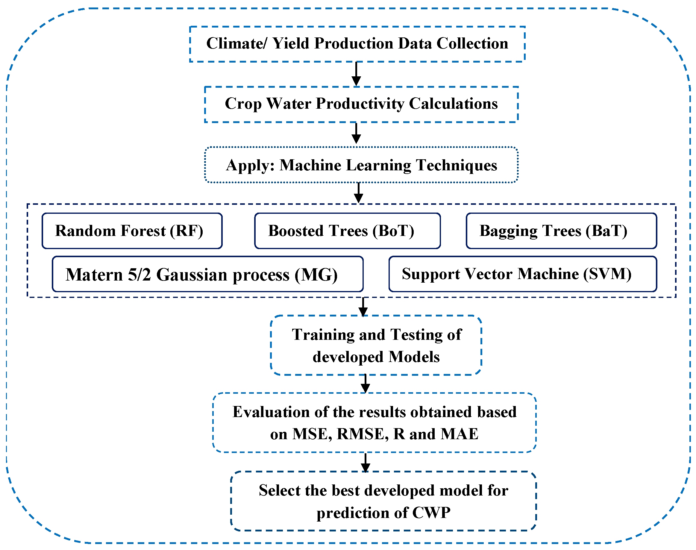
The main skeleton of the study is described in
Figure 1 to highlight the main steps of the study. First, time series climate and wheat and maize grain yield data were collected to calculate CWP. Then, five machine-learning techniques were used to set CWP prediction models using the calculated CWP and other meteorological data. The models’ performances were evaluated, and the best-performing models were identified.
2.1. Study Area
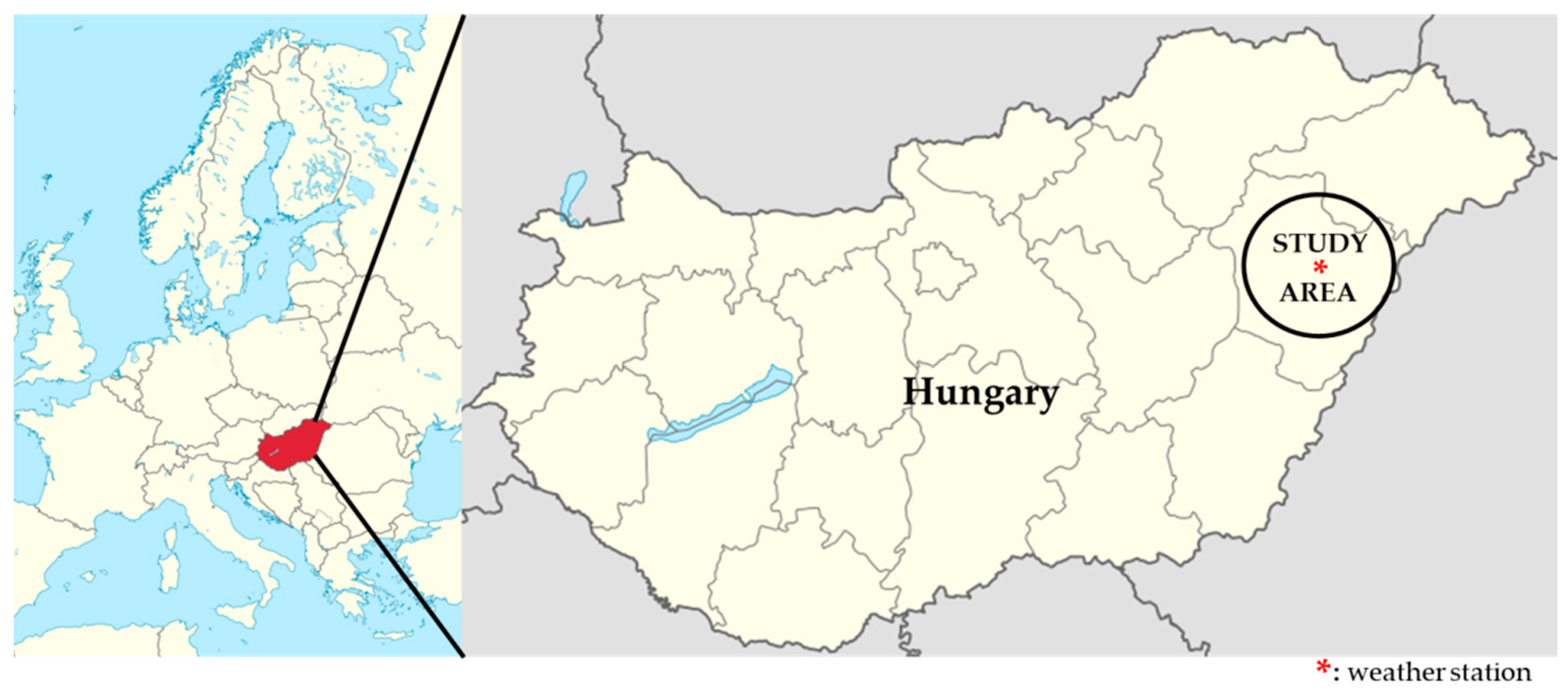
The study area is situated in the eastern part of Hungary (Hajdú-Bihar County), between 47.5° N and 21.6° E (
Figure 2) [
24], as a part of the plains (altitude between 88–153 m) of the Tisza River international catchment. In the Carpathian Basin and Central Eastern Europe, the watershed is the most significant area for the production of wheat and maize. According to the annual reports of the Hungarian Central Statistics Office, maize and wheat are grown on about 55% of the country’s arable land. Therefore, knowledge of winter wheat and maize water productivity is paramount for sustainable cropping and intensification of wheat and maize production.
Three fundamental climatic factors, light or radiation, temperature, and soil moisture, influence vegetation growth and flowering in agricultural production. As a result of the long photoperiod (2050 h year
−1, with 810 h in summer and 175–180 h in winter, the mean annual global radiation of the Tisza catchment’s lowland is relatively large: 4430 MJ m
−2 year
−1 onto the surface. The annual average temperature is 9.6–9.8 °C in Hungary and 17.5 °C in the vegetation period. Based on the climatic dataset of more than 110 years, the research site experiences predominantly northeastern winds with 3 m s
−1 average wind speed. An average of 122 days per year had winds greater than 10 m s
−1. Despite having a continental climate with average annual precipitation of 495 mm and around 350 mm in the vegetation period from 1t April to 30 September, the research site suffers from extreme weather conditions. Events such as droughts, floods, and excess water are frequent issues. Inland excess water and agricultural drought regularly develop in the same year, even in the same vegetation period. The most uncertain climate element is the precipitation at the study site; its annual and seasonal distribution is likewise wildly diverse [
24]. For instance, the highest and minimum annual precipitation was 953 mm and 321 mm, respectively, between 1901 and 2010, according to data from the Hungarian Meteorological Service. The average annual potential evapotranspiration was 918 mm year
−1, where it was 883 mm year
−1 in the first decade of the 1900s and 953 mm year
−1 in the first decade of the 2000s.
The number and lengths of heat waves are also increasing, especially in the flowering and yielding periods of crops. Such heat waves and decreased precipitation can result in severe yield loss and a decrease in crop quality [
25]. The Tisza River Basin is expected to suffer more severe drought events in the future, but more intense precipitation events are also predicted. As a result, the water supply is uncertain; therefore, agricultural and fruit production are vulnerable.
2.2. Data Used
The historical meteorological data recorded in Debrecen (47.532229, 21.624289) for the region of 329,800 ha arable land were downloaded and used in this study. The source of the spatial data is the Research Institute of Agricultural Economics of the National Agricultural and Innovation Centre [
26]. The weather station is situated in the suburban zone of Debrecen city in the middle of a major crop production region. The weather station was set as a reference site as described by Allen et al. [
27] and is part of the official station network of the Hungarian Weather Service. The daily homogenized, filtered, reviewed, and pre-processed (outliers removed) data of minimum temperature (Tmin), maximum temperature (Tmax), mean temperature (Tmean), humidity (H), solar radiation (SR), sunshine hours (Ssh), and wind speed (WS), were downloaded from an open access meteorological database provided by the Hungarian Meteorological Service (
https://odp.met.hu/climate/station_data_series/, accessed on: 14 May 2020) over the long-term period from 1969 to 2019. All data were measured data. Day length (DL) data were calculated using latitude and the calendar day. Out of all meteorological parameters, sunshine hours and solar radiation have been measured with a sparse sensor network (40–60 km distance) since 1969. There are 46 solar radiation sensors that have been working recently [
28]. The spatial extendibility and interpretability of results is always determined by the data with the worst spatial resolution, therefore due to the spatial density of available solar radiation data, a study area can be extracted in a 30 km radius around the meteorological station. On the other hand, the larger the study area is, the larger the smoothing on heterogeneity of other spatially more variable parameters [
29] (e.g., precipitation) which can have a local effect on CWP will be.
The annual average grain yield data of winter wheat and maize were also downloaded from the period of 1969–2019. The official reported yield values were published by the Hungarian Central Statistical Office for the corresponding Nomenclature of Territorial Units for Statistics (NUT) 3 region [
30]. The databases were homogenized and validated with no data gaps. In the previous 20 years, yields were higher than the average of 6.7 t ha
−1 for maize and 4 t ha
−1 for winter wheat only in five cases (2001, 2004, 2005, 2008, and 2014). In 2006 and 2011, yields remained on average. However, the site suffered from drought, especially in several years, 2000, 2002, 2003, 2007, and 2012, when the yield loss of maize was larger than 3 t ha
−1, and severe wheat yield loss (1–1.5 t ha
−1) was also detected. These results agree with the (Standard Precipitation Index) SPI values and meteorological data. The only exception was 2010, when despite extremely high precipitation (900–1300 mm/year), yield quantities remained average due to the abundant surplus water coverage on crop fields and related plant diseases [
25].
Regarding soil conditions, loamy and loamy clay soils dominate maize and wheat cropping lands. The study site is primarily in rain-fed conditions with 100–110 kg ha−1 nitrogen active substance utilization. Cultivars are also crucial in CWP. On the other hand, due to the size of the study area, no data are available for cultivars; therefore, it was not possible to consider the effect of cultivars on CWP.
Cropping practices are dominantly rain-fed. Only 2% of the agricultural land is irrigable in Hungary and the study area region due to technical reasons. Based on the Hungarian Central Statistical Office, the ratio of the irrigated arable land varied between 0.59–5.9% in the study region in the previous decades depending on the rainfall characteristics [
31]. Furthermore, under irrigation, sweetcorn and other types of crops are grown [
32]. In Hungary, the grain maize and wheat were not irrigated in the investigated period of time [
33].
It has to be noted that due to spatial coverage and the properties of the study site described above, the modeling is focusing on a regional scale since it cannot cover and consider local field scale variations in yields or other meteorological parameters.
2.3. Calculation of Crop Evapotranspiration
The study estimated the reference crop evapotranspiration (ET
o) using the Hargreaves method Equation (1) by the Food and Agricultural Organization (FAO). Since the present study’s focus was more inclined toward developing models with limited climate data, relatively higher data-demanding methods such as Penman–Monteith (PM) were not considered for predicting reference evapotranspiration and, thereby, crop water productivity [
34,
35,
36,
37,
38,
39]. The Hargreaves method (HM) only requires minimum and maximum temperatures and solar radiation data. ET
o was calculated based on the climatic data of the weather station data of Debrecen. The crop evapotranspiration ET
c was calculated using the simple Equation (ET
c = ET
o × K
c), based on calculated ET
o and standard K
c values defined by FAO 56 paper [
27].
where T
mean is the daily average temperature (°C), T
max is the daily maximum temperature (°C), T
min is the daily minimum temperature (°C), and R
a is extraterrestrial radiation (mm day
−1).
To adopt FAO K
c values, the phenological stages were adapted to the local climate and cropping circumstances. In the investigated period, 15 April was considered the average sowing, mid- July was the tasseling period, and 30 September was the harvesting time for grain maize, which corresponds to the practice in Hungary [
40]. In accordance with the agricultural practice of winter wheat, the sowing time was set at 5 October, shoot development was between 5 March and 20 May, full flowering was set at 10 June, and harvesting at 10 July [
41].
2.4. Calculation of Crop Water Productivity
Crop water productivity (CWP) was defined as the yield obtained per unit of water consumed [
42] Equation (2).
where Y is the average yield (kg ha
−1) for the study area, and WR is the total amount of water used in the field, which is set equal to
. (m
3 ha
−1) of the cropping periods of maize or wheat in the present study.
2.5. Ensemble Machine Learning
Yield, meteorological data, and calculated ETc were considered in this study to set CWP prediction models. In model building, to take advantage of long-term time series datasets for CWP, the present study categorized the complete dataset into two sets, of which, the first segment comprised 76.5% of the dataset for training purposes (for the training period 1969–2007), while the second segment comprised 23.5% for validation/testing purposes (for the testing period 2008–2019) of the models.
2.5.1. Random Forest (RF)
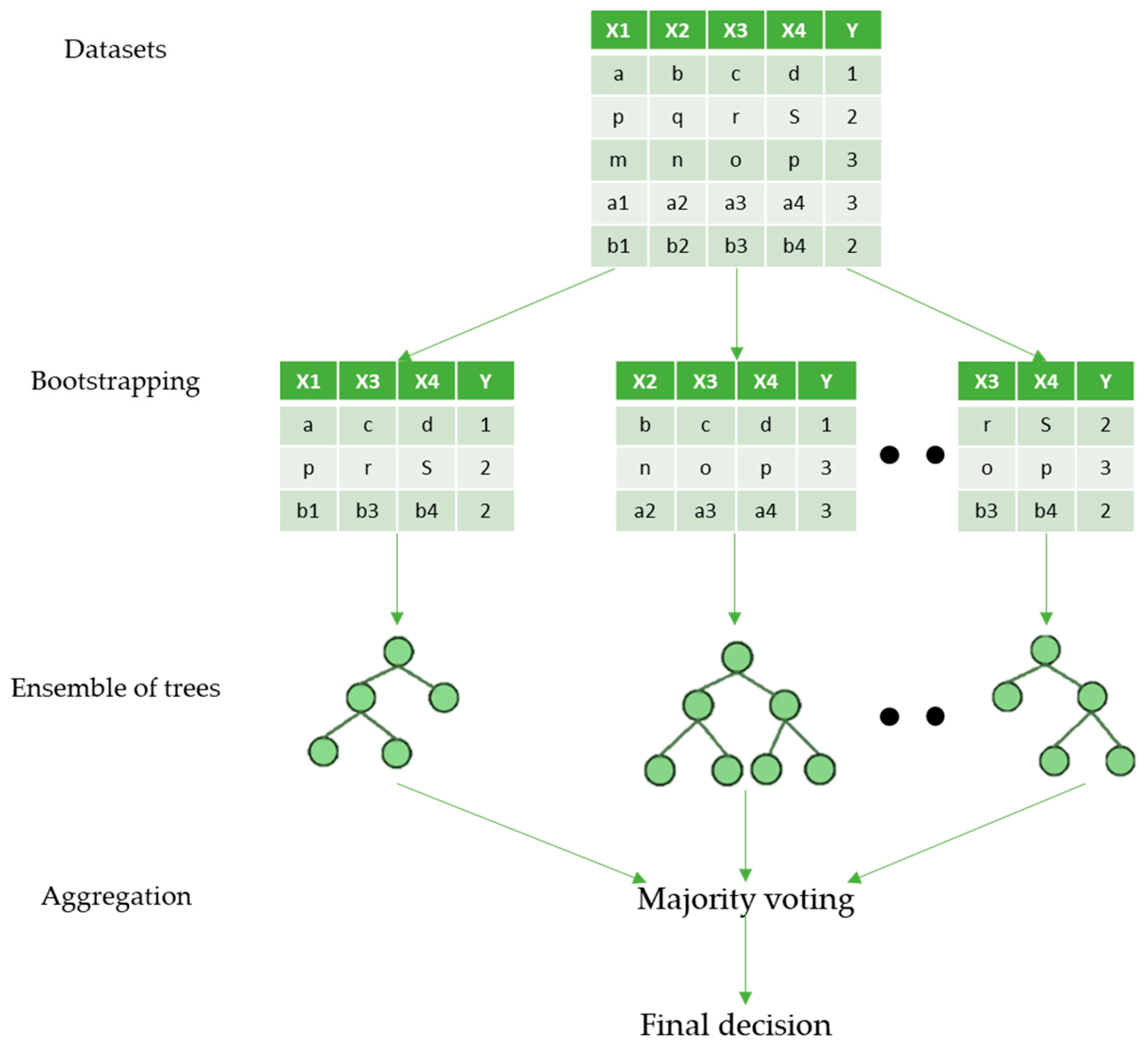
Random forest (RF) is an ensemble method that applies numerous decision trees in parallel with the bagging (bootstrapping followed by aggregation) approach (
Figure 3). Bootstrapping implies the simultaneous training of several separate decision trees on varying subsets of the input training dataset. The RF model yields comparatively higher performance while constructing ensembles. The learning algorithms of decision trees rely on a classification and regression tree (CART). Considering the architecture, RF comprises sets of decision trees, wherein space occupied by each variable is further sub-divided into smaller and smaller sub-spaces, achieving uniform space for each data/variable. The structure of decision tree is employed for this classification pattern such that two sub-branches originating from a branching point are recognized as a node. In the tree structure, the root is identified as the first node, and the leaf is identified as the last node [
19]. Each of these trees develops with a self-serving sample of the original data. To achieve the best division, a variable, randomly selecting the ‘m’ number of variables, is searched [
43]. RF measures high-level predictive parameters and provides precise and exact outcomes using a powerful artificial intelligence technique without overfitting issues [
19,
43,
44]. This decreases the model’s total variance and gives reliable findings [
45]. As a final step in the decision process, the decisions of individual trees are aggregated for better generalization [
46]. The strength of the individual tree combinations and their degree of correlation determines the random forest’s generalization error. Random forest models have been demonstrated to be robust predictors and versatile for both classification and regression problems involving small sample sizes and high dimensional data [
47]. The major advantages of the RF technique are its capacity to generalize, lower sensitivity to attribute values, and built-in cross validation [
48]. The selected parameters for implementing this method were Batch size 100, bag Size percent = 100, max depth = 0, number of executions slots = 1, number of iteration = 100, and random seed = 1.
2.5.2. Support Vector Regression (SVR)
The support vector regression (SVR) approach is a novel learning machine and appears promising. SVR is based on the structural risk minimization approach and statistical learning theory, previously applied to data categorization, regression, and non-linear systems modeling [
49]. Detailed descriptions of SVR can be found in Vapnik, Schölkopf, and Smola’s studies [
49,
50]. The parameters used in this method were batch size-100, C = 0.1, kernel used = polykernel.
2.5.3. Bagged Trees
The primary idea behind bagged trees (BT) is that instead of relying on a single decision tree, you rely on many of them, allowing you to combine the insights of multiple models. As a result, ensemble methods can consider the generalization of the model to new datasets when an algorithm overfits (high variance and low bias) or underfits (low variance and high bias) to its training set [
51]. In this context, the current investigation used a random sample of data from a training set with replacement. The models resulting from this were limited since on an individual basis their performance may not be substantial due to a large variation or substantial bias. This enabled the selection of certain data points multiple times. After receiving many data samples, these unreliable models were trained independently using regression and classification. Overall, aggregating these poor models enabled lower biases and variances, yielding improved model performance. The features used in this method were batch size 100, bag size percent = 100, classifier = REPTree, max depth = 0, number of executions slots = 1, number of iterations = 10, and random seed = 1.
2.5.4. Boosted Trees
Boosted tree (BoT) is a machine learning approach for prediction research that builds a model in the form of an ensemble. BoT simplifies the loss function’s random differences for optimizing the stages’ multiple levels. Following that, the gradient boosting technique was developed to maximize the cost function and iteratively choose function points in the negative gradient direction [
52]. Each base model generates a unique tree model by bootstrapping a sample from the training data and then segmenting the feature space into region sets. A simple model is then fitted to each region. Sreedhara et al. [
53] describe the method used in this study in detail. The features used in this method were batch size 100, classifier = REPTree, max depth = 0, number of executions slots = 1, number of iterations = 10, and random seed = 1.
2.5.5. Matern 5/2 Gaussian Process
A Gaussian process (GP) is an infinite group of random variables with a constant joint Gaussian distribution in any finite subsets [
54,
55,
56]. A mean function and a covariance function are used to represent a GP. The mean function is commonly considered zero because the GP is a linear combination of random variables with a normal distribution. GP captures model uncertainty directly; for example, it provides a distribution for the predicted value instead of a single value as the prediction in regression. This uncertainty is not explicitly captured in neural networks. By employing different kernel functions, GPR incorporates prior knowledge and requirements regarding the model’s geometry. The matern 5/2 Gaussian process is detailed in the Asante-Okyere et al. [
57] study. The proposed features for this method were kernel= PUK; batch size-100, noise = 1, seed = 1; filter type = normalize training data; cache size = 250,000; omega = 1, sigma = 1.
2.6. Performance Metrics and Evaluation
Calculated data of CWP were compared to modeled values using data from this study’s investigation period. Model performances were evaluated using mean square error (MSE) Equation (3), root mean square error (RMSE) Equation (4), coefficient of determination (R
2) Equation (5), and mean absolute error (MAE) Equation (6) [
58]. The MSE in this study assesses the quality of an estimator (i.e., a mathematical function mapping a sample of data to an estimate of a parameter of the population from which the data are sampled). RMSE is the sample standard deviation of the differences between predicted and actual values. The mean absolute error evaluates the mean magnitude of the errors in predictions without considering their sign. The reason behind employing RMSE is its ability to measure accuracy so as to compare predicting errors of varying models for a particular dataset and not between datasets. The study used R
2 because it provides a measure of how well the predicted future is replicated by the model based on the variability from the actual values. MAE provides the mean of the absolute errors (between the forecasted value and the actual value), such that it allows determining how huge an error can be expected from the forecast on average.
where
is an observed calculated value,
is simulated value,
is the mean value of reference samples, and N is the total number of data points.
3. Results
3.1. Correlation Analysis
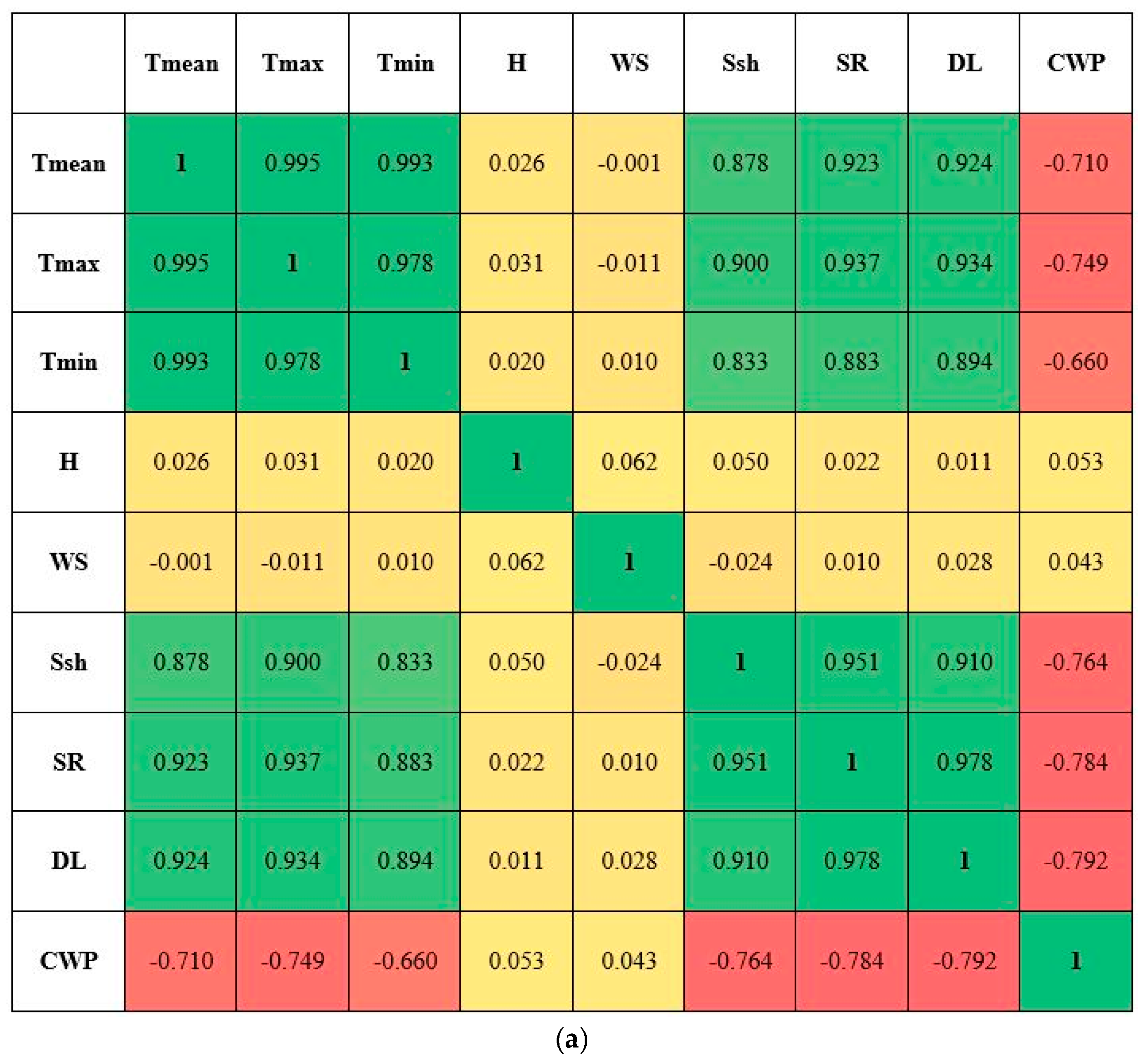
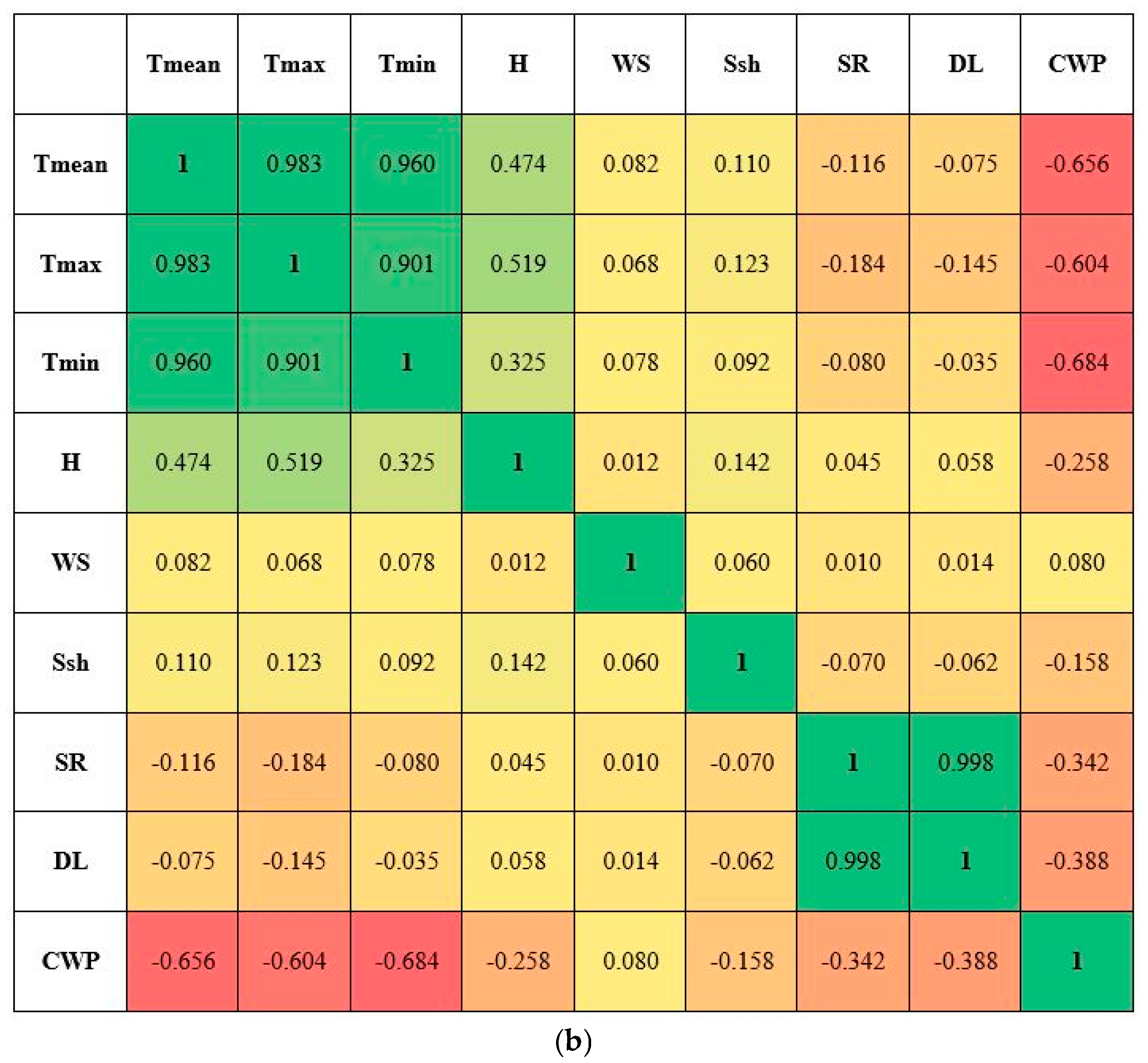
This study conducted correlation analysis to ascertain correlations between a dependent variable (CWP) and independent variables (Tmean, Tmax, Tmin, WS, H, Ssh, SR, and DL) and also between independent variables for wheat and maize, as shown in
Figure 4. In general, the study recorded significantly higher correlations between independent variables such as Tmean, Tmax, Tmin, SR, Ssh, and DL. In the case of wheat (
Figure 4a), temperature variables (Tmean, Tmax, and Tmin) recorded a positive correlation with temperature variables along with Ssh, SR, and DL; however, negative or near positive correlation was observed with H, WS, and CWP. It is imperative to highlight here that both H and WS recorded a positive correlation with CWP. In the case of maize (
Figure 4b), temperature variables (Tmean, Tmax, and Tmin) recorded a positive correlation with temperature variables along with H, WS, and Ssh (except for Ssh, this correlation is apparently different from the case of wheat); however, negative or near positive correlation was observed with WS and CWP. It is to be distinguished here that both H and WS (same as in wheat) recorded a positive correlation with CWP.
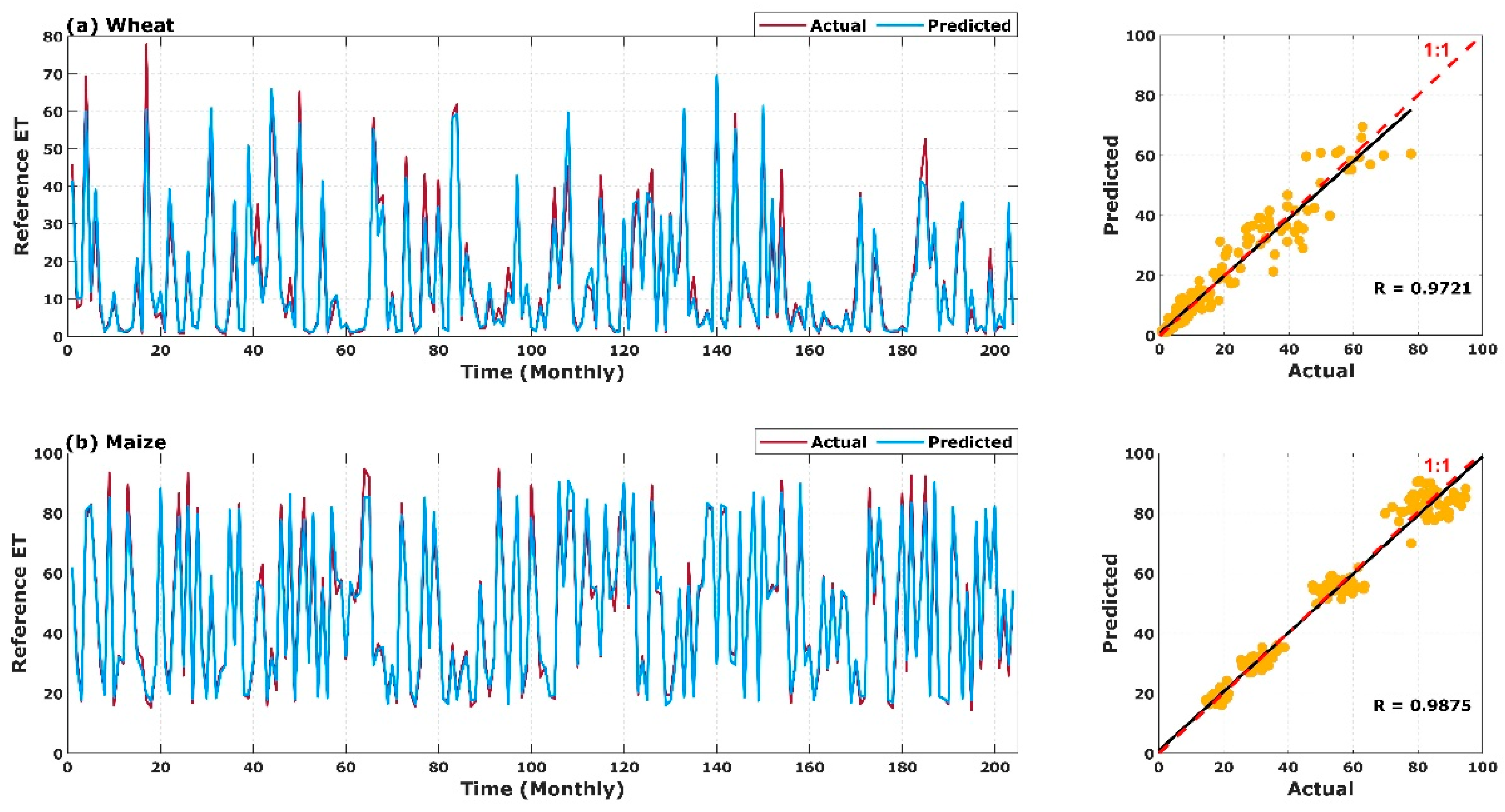
3.2. Validation of ET Values
Furthermore, it was essential to validate the actual crop evapotranspiration magnitudes with their actual values. Consequently, the present investigation conducted cross validation between actual and predicted magnitudes of reference crop evapotranspiration to ascertain an acceptable correlation between them.
Figure 5 shows cross-validation results for wheat and maize crops. Findings indicated a very high correlation between the actual and predicted values recording 0.972 for wheat and 0.987 for maize. Hence, the study found models suitable for conducting crop water productivity estimations (described in the following sections).
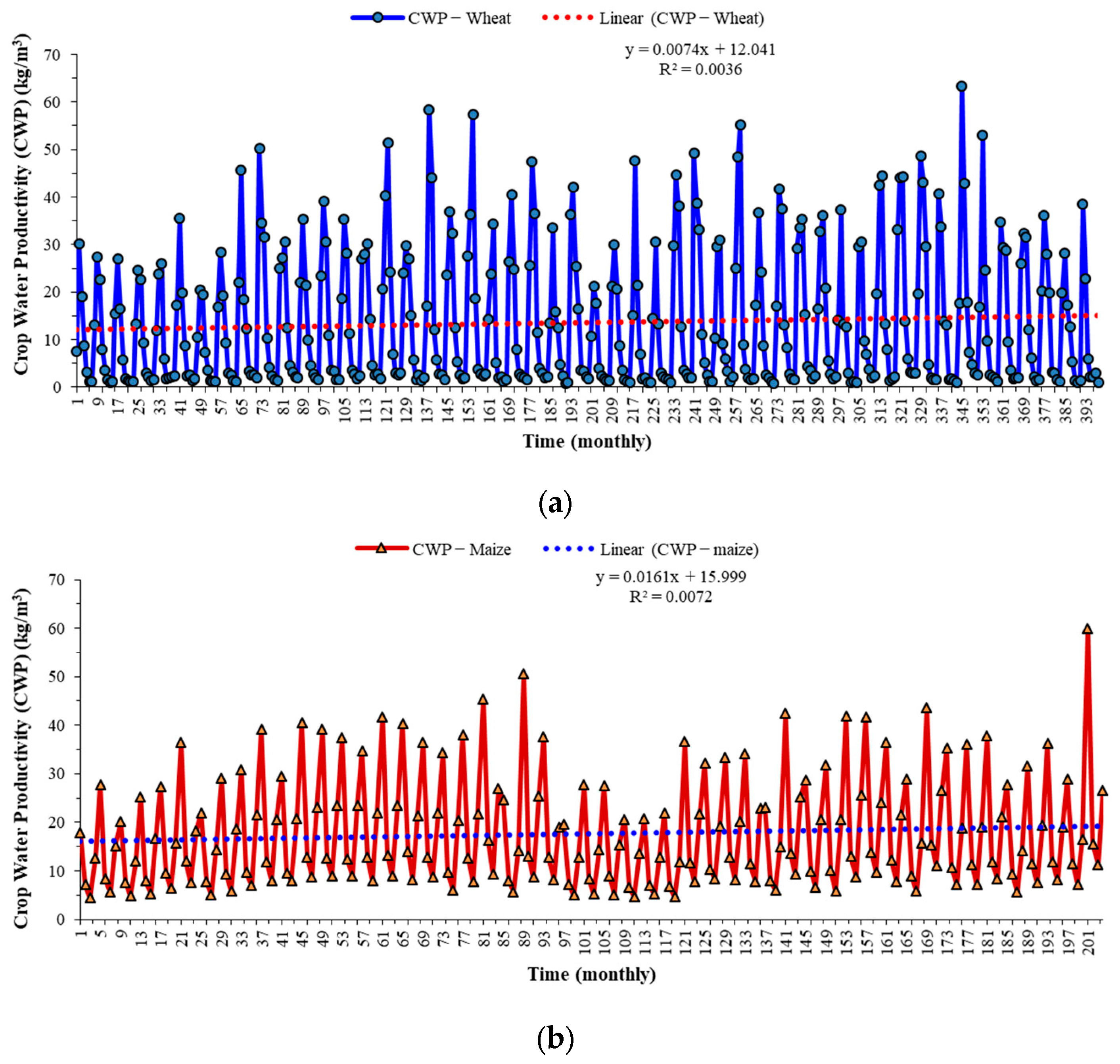
3.3. Trend Analysis for Wheat and Maize CWP
The findings from correlation analysis directed for plotting the WP magnitudes for the period 1969–2019 for both wheat and maize. This is calculated to ascertain the anomalies from the trend analysis of wheat and maize for CWP.
Figure 6 shows the time series of CWP for wheat and maize for the study period 1969–2019.
In the case of wheat, an increasing trend of CWP is observed, as inferred from its trend equation (y = 0.0074x + 12.041) (
Figure 6a). The increasing trend reveals an improvement in the crop water productivity for wheat in the last five decades. Regarding the extremities, the maximum CWP value was obtained as 63.33 kg m
−3, while the minimum CWP value was recorded as 0.84 kg m
−3. In general, the average CWP value for the entire study period was recorded at 13.52 kg m
−3 with a standard deviation of 14.25 kg m
−3, whereas the maize crop too observed an increasing trend of CWP, as inferred from its trend equation (y = 0.0161x + 15.999) (
Figure 6b). It is imperative to distinguish here that in either case, the trend was observed as positive, but it was greater for maize than wheat. The increasing trend here, too, reveals an improvement in the maize crop water productivity, especially during the last five decades. Regarding the extremities, the maximum CWP value was obtained as 59.84 kg m
−3 (less than wheat), while the minimum CWP value was recorded as 4.41 kg m
−3 (greater than wheat). In general, the average CWP value for the entire study period was recorded at 17.65 kg m
−3 (which is far greater than wheat) with a standard deviation of 11.57 kg m
−3 (indicating less variation from the mean value as compared to wheat).
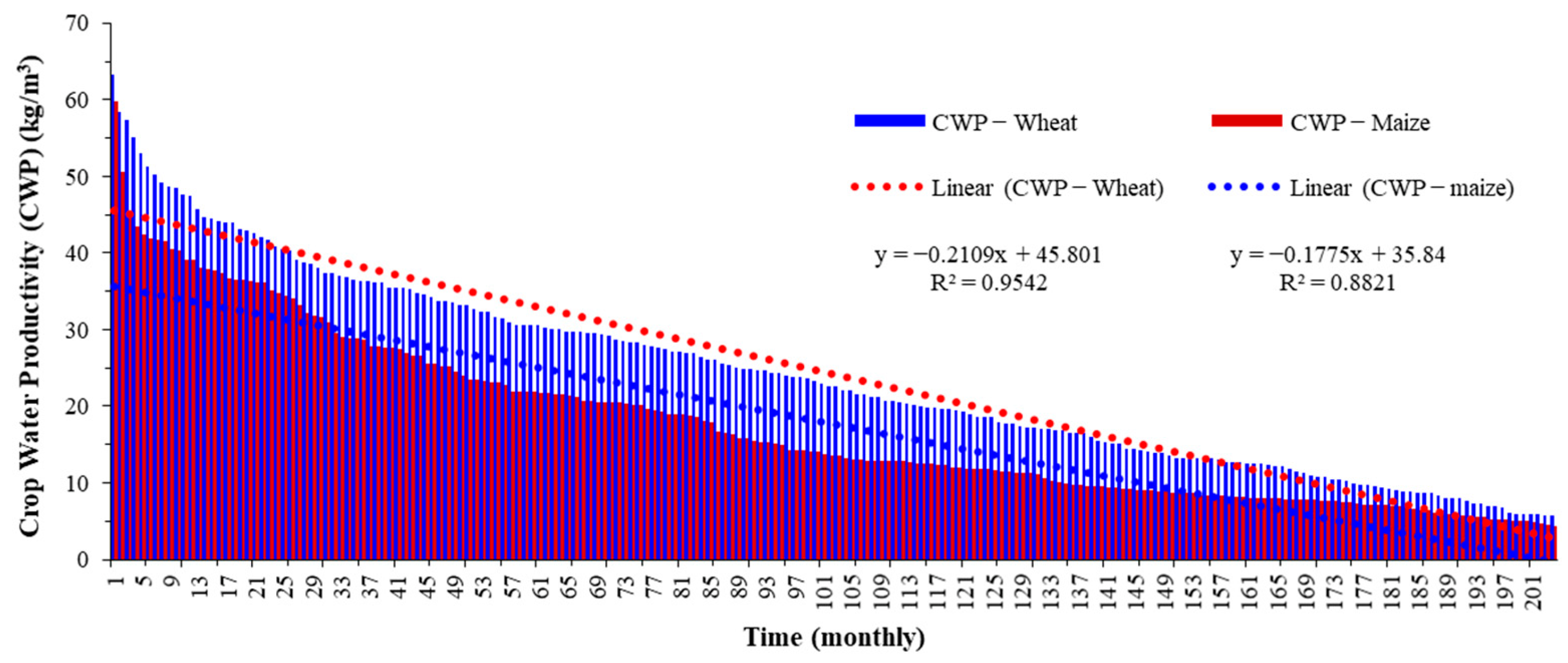
To further compare wheat and maize CWP, time series was plotted in the sequence from higher to lower CWP values for both wheat and maize (
Figure 7). The R
2 value obtained was higher for wheat (0.95) than maize (0.88) when the series were compared with their corresponding linear trend. It is evident here that the CWP values have always remained higher for wheat than maize in the last five decades. To quantify this, similar statistical parameters were estimated as was done for wheat and maize time series for CWP. The average percentage difference for CWP between wheat and maize was obtained as 43.23% with a standard deviation of 16.03%, indicating that wheat remained higher for CWP magnitude than maize by an average of 43.23% between 1969 and 2019. The maximum and minimum percentage difference during the entire study period for CWP magnitude of wheat and maize was recorded at 70.96% and 5.83%, respectively. It is imperative to determine which field conditions, such as irrigation techniques, etc. (apart from climatological aspects covered in this study), have made wheat CWP far higher than maize crops. However, conducting this investigation is beyond the scope of the present objectives. Hence, this study urges future researchers to direct investigation on understanding the irrigation and water supply–demand management aspects for wheat cropping in the study area. Findings can be useful for developing the best irrigation management practices.
3.4. Data Fusion of Climatic Factors for Modeling CWP for Wheat and Maize
The different combinations of input variables provided the performance of the models such that some combinations yielded positive contributions to the accuracy, while some yielded negative contributions under each case of the selected models (also described in the next section). The best influential variables against each model type (Model 1 to Model 10), so as to identify the best performance of the models in modeling the CWP with greater accuracy, are shown in
Table 1. These models were developed using machine learning algorithms, viz., RF, SVM, BT, BoT, and MG. Model 8 comprised maximum independent variables (Tmax, Tmin, Tmean, SR, WS, H, DL, and Ssh) followed by Model 1 (Tmax, Tmin, Tmean, WS, H, and Ssh), while Model 9 comprised minimum independent variables (Tmean and SR) followed by Model 10 (Tmax, Tmin, and Ssh). To evaluate the performances of the applied algorithm, four performance indicators were employed, viz., coefficient of determination (R
2), mean square error (MSE), root mean square error (RMSE), and mean absolute error (MAE).
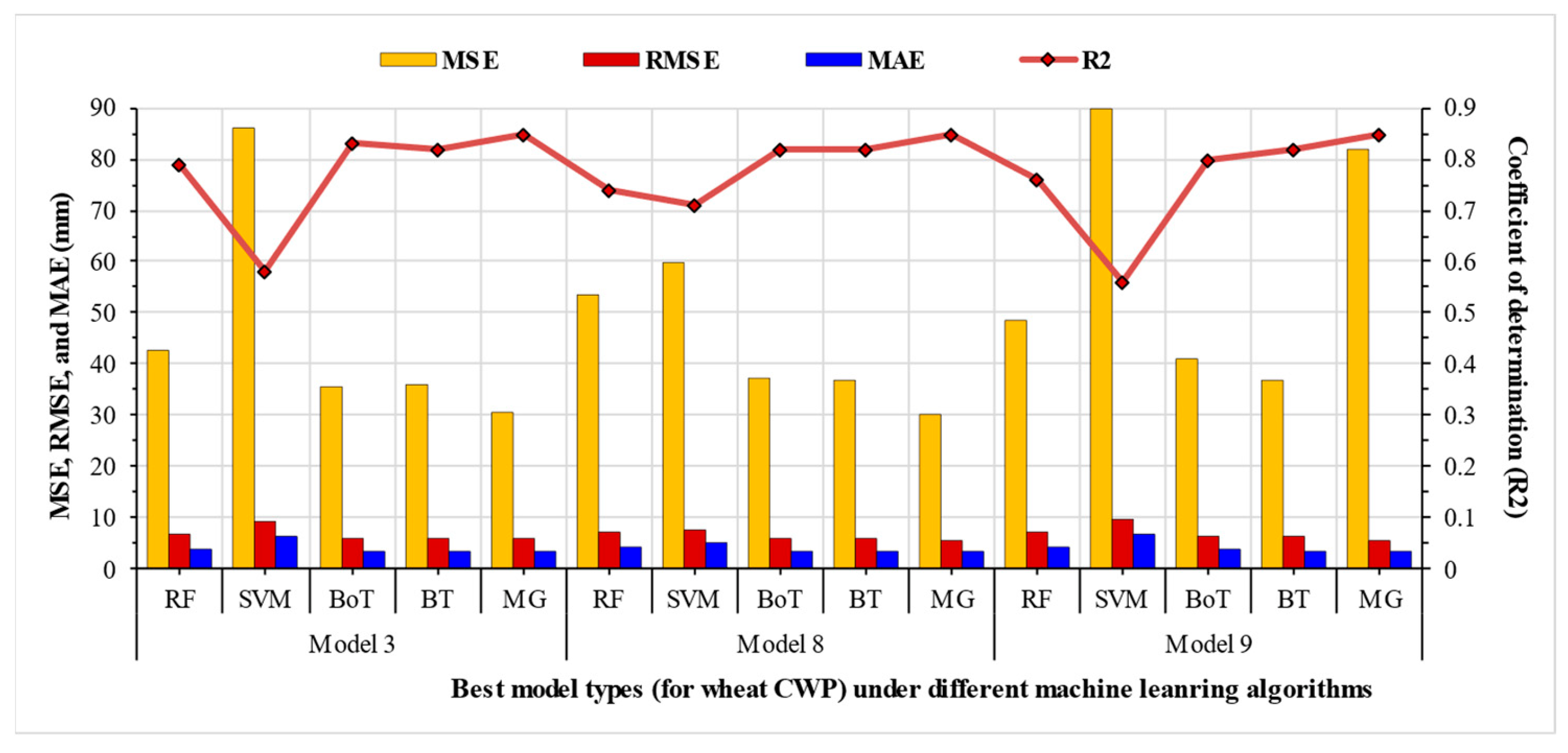
3.5. Evaluation of Machine Learning Models for Estimation of CWP for Wheat
As discussed, CWP for wheat was estimated by implementing an ensemble of five machine learning algorithms, viz., RF, SVM, BT, BoT, and MG. The best performance of the models was identified based on the higher value for R
2 (close to one) and lower values for MSE, RMSE, and MAE (close to zero).
Table 2 shows the general trend for these performance indicators corresponding to each model. By following the aforesaid criteria of performance quantification, Model 3, Model 8, and Model 9 were observed as the best models during both the training and testing phases (refer to
Figure 8).
In the case of Model 3, the best algorithm was MG which demonstrated the most appropriate values for all model evaluation metrics as compared to the other four algorithms. This was followed by BoT and then BT. While in the case of Model 8, the best algorithm was also MG, which demonstrated the most appropriate values for all model evaluation metrics. However, this was followed by BT and then BoT (in contrast to the Model 3 pattern). Nevertheless, in the case of Model 9, the best algorithm was also MG, which demonstrated the most appropriate values for all model evaluation metrics except for MSE values (recorded higher than BT, BoT, and RF), as compared to the other four algorithms. Similar to Model 3, MG was followed by BT and then BoT. In general, RF and SVM remained satisfactory algorithms; BT and BoT performed better than RF and SVM, while MG performed the best.
As far as the selection of the most optimal model is concerned, Model 8 was observed to be the best, with the highest average values for R2 (0.79) and lowest values for MSE (43.5 kg m−3), RMSE (6.47 kg m−3), and MAE (3.85 kg m−3); followed by Model 3 with R2 (0.77), MSE (46.12 kg m−3), RMSE (6.71 kg m−3), and MAE (3.95 kg m−3); and then Model 9 with R2 (0.76), MSE (59.62 kg m−3), RMSE (6.91 kg m−3), and MAE (4.21 kg m−3).
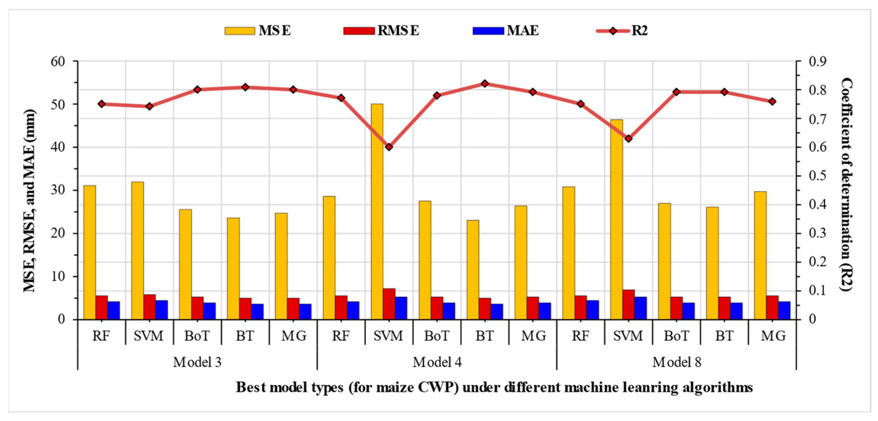
3.6. Evaluation of Machine Learning Models for Estimation of CWP for Maize
The general trends for model evaluation performance metrics (R
2, MSE, RMSE, and MAE) of CWP for maize, corresponding to each model (RF, SVM, BT, BoT, and MG), are shown in
Table 3. By following the criteria of performance quantification, as was discussed in the previous subsection, Model 3, Model 4, and Model 8 were identified as the best models during both the training and testing phases (
Figure 9).
In the case of Model 3, the best algorithm was BT which demonstrated the most appropriate values for all model evaluation metrics as compared to the other four algorithms. This was followed by MG and then BoT. Similar to Model 3, Model 4 also identified BT as the best algorithm, followed by MG and then BoT. In the case of Model 8, the best algorithm was also BT which demonstrated the most appropriate values for all model evaluation metrics. Unlike Model 3, and Model 4, in Model 8, BT was followed by BoT first and then MG. In general, similar to the wheat crop, in the case of the maize crop too, the RF and SVM remained satisfactory algorithms; However, instead of BT in the wheat crop, MG and BoT were observed performing better than RF and SVM, while BT was observed performing the best (against the MG in the case of the wheat crop).
As far as the selection of the most optimal model is concerned, Model 3 was observed to be the best, with the highest average values for R2 (0.78) and lowest values for MSE (27.36 kg m−3), RMSE (5.22 kg m−3), and MAE (3.82 kg m−3); followed by Model 4 with R2 (0.75), MSE (31.03 kg m−3), RMSE (5.51 kg m−3), and MAE (4.02 kg m−3); and then Model 8 with R2 (0.74), MSE (32.01 kg m−3), RMSE (5.62 kg m−3), and MAE (4.21 kg m−3).
4. Discussion
The present study attempted to test various (ensemble) machine learning algorithms and their predicting capability of CWP values for wheat and maize crops in the study site, Debrecen (eastern part of Hungary). More or less, the findings for RF, SVM, BT, BoT, and MG models demonstrated high predicting abilities in estimating CWP values. To further emphasize the reason behind choosing the algorithms mentioned above, their high performance amidst an excellent learning ability for complex and highly non-linear relationships made them excellent candidates for our study. Comparatively, this study found MG as the best model for the wheat crop and BT as the best model for the maize crop so as to advance future investigation in the study area using these models. The models MG and BT were observed to outperform other models by acquiring the most appropriate values for the performance matrix (highest for R2 lowest for MSE, RMSE, and MAE). The time series and scatter plots further ascertained these findings developed for comparing the ensemble of five machine learning algorithms and 10 types of different data fusion-based models (Model 1 to Model 10). They comprehensively indicated that Model 8 was the best model, followed by Model 3 and Model 9 for the wheat crop, and Model 3 was the best model, followed by Model 4 and Model 8 for the maize crop. Herein, it can be seen that Model 3 and Model 8 are common models in wheat and maize crops, indicating more significant superiority and suitability for crop water productivity analysis in the given study area. Furthermore, apart from MG and BT models (best models for wheat and maize crops, respectively), BT and BoT models were observed as the next best category of models in the case of the wheat crop, and MG and BoT were observed as the next best category of models in the case of the maize crop. However, the performance of the remaining two models, viz., RF and SVM, remained merely satisfactory for wheat and crop CWP modeling.
The MG model performed better compared to others, maybe since it is a probabilistic supervised machine learning framework that provides its application in both regression and classification tasks. It can make predictions by incorporating prior knowledge (kernels) and provide uncertainty measures over predictions. As a result, its performance (statistically) was better, at least in the case of crop water productivity predictions, than other employed models. In comparison, the possible reason behind the better performance of the BT model could be its ability to bag many trees. In such a case, it is no longer possible to represent the resulting statistical learning procedure using a single tree. In addition, which variables are most important to the system is no longer clear. Thus, in the present investigation, bagging could improve the prediction accuracy of crop water productivity at the expense of interpretability.
Amidst the ongoing research on estimating crop water productivity, it is imperative to highlight here that the present combinations of an ensemble of five machine learning models, viz., RF, SVM, BT, BoT, and MG for CWP modeling is a novel approach. In addition, the present study determined MG and BT as the most suitable models among the 10 different types of models (Model 1 to Model 10 based on varying influential independent variables) developed in this study. Both these inferences are against the ongoing trend, wherein researchers have primarily focused on estimating plant water stress in wheat and maize using methods other than machine learning algorithms. Limited studies have used machine learning algorithms for estimating crop water productivity or, more precisely, plant water stress. Virnodkar et al. [
59], in their extensive review on determining crop water stress using remote sensing and machine learning further confirmed that no studies are currently available employing RF, SVM, BT, BoT, and MG for wheat and maize water stress estimation. Instead, crop water stress index (CWSI)-based methods remained predominant in their estimation. In an attempt to improve crop water use efficiency, Babaeian et al. [
60] developed a novel approach for root-zone soil moisture estimation based on remotely sensed soil data and automated machine learning. Their investigation found that machine learning is better able to capture measured in situ root zone soil moisture, resulting in a more precise spatial variability of soil moisture at the field scale. Actual evapotranspiration was forecasted by Granata [
61] for developing a more careful assessment schema of irrigation needs using M5P regression tree (RT), BT, RF, and SVM in the central Florida site. The study determined machine learning algorithms were a powerful tool, while requiring accurate predictions in specific and careful management of agrarian water resources in general. Similarly, Kar et al. [
62] used an ensemble of three machine learning algorithms, viz., SVM, artificial neural network (ANN), and RF, to establish one-to-one plant–water relations and generate continuous evapotranspiration profiles. Their study found machine learning techniques yield optimal results with minimum redundancy and information loss. Elbeltagi et al. [
63] developed a novel combined terrestrial evapotranspiration index (CTEI) for the Ganga River Basin in India by employing SVM, decision trees (DT), MG, BoT, and BT, wherein their study found MG along with SVM as the best performing models. In general, all the aforementioned studies have jointly concluded through their various model assessments that the models selected in this study (RF, SVM, BT, BoT, and MG) were observed to be suitable models among many machine-learning-algorithm-based models being used globally.
To recapitulate, ML models need to be used to predict WP based on limited input variables data to maximize irrigation water requirements and increase crop production. It is a new tool, or rather approach, for water users, developers, and decision makers for achieving agricultural sustainability under climate change conditions and limited climate data variables. In addition, since the present approach is one of the first of its kind, it was required to compare the findings from this study with the results of other different approaches in the literature to emphasize the need for the present study. Consequently, the ML models used in this study lack their applications in crop water productivity estimation in the scientific literature; hence, our study remained more focused on exploring the model’s ability. Moreover, the present study finds its significance in giving direction to coupling agricultural investigations in view of estimating crop water productivity with machine learning algorithms. Amidst climate change, the unsustainable land use land cover changes and their negative impact on the agricultural land cover aggravate recurring floods [
64,
65] and chronic droughts [
66,
67]. Therefore, 21st century agricultural research demands an improved understanding of various agrarian water use aspects, such as soil moisture availability, irrigation capacity, crop water requirements, consumption, etc.
5. Conclusions
Modeling crop water productivity to maximize water use has been increasing. This study used ensemble machine learning to determine the best crop water productivity (CWP) prediction and simulation model for wheat and maize. As the main finding, the optimal regional scale models for forecasting CWP of wheat can be implemented by MG with the following weather combinations: (i) involving parameters of Tmean, SR, WS, and DL implemented by MG, (ii) using Tmax, Tmin, Tmean, SR, Ssh, WS, H, and DL; or (iii) calculating with Tmean and SR. The best prediction for maize CWP can be modeled by BT using a combination of: (i) SR, WS, H, and Tmin data, (ii) Tmax, Tmin, Tmean, SR, Ssh, WS, H, and DL, and (iii) Tmean, SR, WS, and DL. Consequently, the present investigation devised a machine learning-based approaches for ascertaining water productivity. Our results indicate that knowledge of machine learning algorithms becomes paramount, especially when their current application in agrarian water consumption and corresponding efficiency estimation for primary crops is limited. The results also suggest that in the case of limited climate data, there are solutions to predict the CWP of wheat and maize. The selected models achieved high performance and fewer residual errors. Thus, the models provide a rapid decision tool in regional scale CWP prediction and can help promote decision making for water managers, designers, and development planners. Such investigations may allow estimating the future magnitudes of water consumption and efficiency aspects precisely, thereby alarming the concerned authorities and administrators for early detection of crop water stress and orienting their decision making towards more specific sustainable agriculture.


 ,
, 


