Prediction of Sediment Yield in a Data-Scarce River Catchment at the Sub-Basin Scale Using Gridded Precipitation Datasets

Abstract

Water-related soil erosion is a major environmental concern for catchments with barren topography in arid and semi-arid regions. With the growing interest in irrigation infrastructure development in arid regions, the current study investigates the runoff and sediment yield for the Gomal River catchment, Pakistan. Data from a precipitation gauge and gridded products (i.e., GPCC, CFSR, and TRMM) were used as input for the SWAT model to simulate runoff and sediment yield. TRMM shows a good agreement with the data of the precipitation gauge (≈1%) during the study period, i.e., 2004–2009. However, model simulations show that the GPCC data predicts runoff better than the other gridded precipitation datasets. Similarly, sediment yield predicted with the GPCC precipitation data was in good agreement with the computed one at the gauging site (only 3% overestimated) for the study period. Moreover, GPCC overestimated the sediment yield during some years despite the underestimation of flows from the catchment. The relationship of sediment yields predicted at the sub-basin level using the gauge and GPCC precipitation datasets revealed a good correlation (R² = 0.65) and helped identify locations for precipitation gauging sites in the catchment area. The results at the sub-basin level showed that the sub-basin located downstream of the dam site contributes three (3) times more sediment yield (i.e., 4.1%) at the barrage than its corresponding area. The findings of the study show the potential usefulness of the GPCC precipitation data for the computation of sediment yield and its spatial distribution over data-scarce catchments. The computations of sediment yield at a spatial scale provide valuable information for deciding watershed management strategies at the sub-basin level.

1. Introduction

Appropriate measures for watershed management require precise prediction of sediment yield from the catchment. Precipitation is the key element for simulating runoff and sediment load at the catchment scale. Spatial variability of rainfall events is a major limitation for reliable estimations of runoff and sediment yield in large catchments. Moreover, sediment load in rivers is affected by many factors, including soil type, land use, channel slope, catchment area, seasonality of rains, land sliding, etc. Therefore, reliable estimates of runoff and sediment yield from catchments require considerably accurate input datasets, especially the precipitation, which plays an important role. Erratic rainfall events in arid and semi-arid regions having barren land with dendritic drainage patterns cause major off-site effects, including decreases in reservoir storage capacity and sedimentation in the irrigation infrastructure [1]. The sedimentation in reservoirs increases with the high erosion rates in catchments, thus reducing the storage capacity of dams and decreasing irrigation supplies to the canal system. For example, the storage capacity of Warsak Dam’s reservoir in Pakistan was reduced by 18% during the first year of its operation. Similarly, the storage capacities of Tarbela, Mangla, and Chashma reservoirs were reduced by 35, 20.5, and 60%, respectively [2]. For the Indus Basin Irrigation System (IBIS), Pakistan, irrigation supplies can decrease by 20% during the Rabi cropping season (Nov. to March) due to sedimentation in the reservoirs under climate change scenarios [3].

The Gomal River catchment and the Northern parts of Pakistan are particularly vulnerable to high erosion rates, i.e., >50 tons ha^–1 year^–1 [4]. In a recent study [5], the erosion rates in the sub-catchment of the Gomal River were categorized as being in a range from very severe to catastrophic (i.e., >100 t h⁻¹ y⁻¹). The eroded sediment from the Gomal River basin reaches the reservoir of the Gomal Zam (GZ) dam and periodically sluices in the downstream river reach. These highly sediment-laden flows from the dam outlet ultimately reach the Kot Murtaza Barrage (≈40 km downstream of GZD). Moreover, the runoff during rainfall events from the sub-basin between GZD and the Kot Murtaza Barrage also results in significant sediment load, which is ultimately diverted into the irrigation canal [5]. However, the relative contribution of sediment load at the Kot Murtaza Barrage from the sub-basin is unknown due to the unavailability of a data monitoring station at the dam site. The importance of Kot Murtaza Barrage is due to its newly developed irrigation network, which irrigates about 77,000 ha of agricultural land. Therefore, sediment load assessment from the catchment area can play a vital role in devising appropriate management strategies.

Hydrological models are widely used for the assessment of runoff and sediment yield from the catchments. These models use different types of information including topography, soil type, land management practices, and precipitation. The physically based semi-distributed model ‘SWAT’ has been widely used worldwide for diverse river basins for successfully simulating runoff and sediment yield [6,7,8,9,10]. The model uses terrain, soil, land use, and climate data as input for simulation. The most important input to the model is the precipitation due to its temporal and spatial variability. Obtaining precipitation information presents a serious challenge for data-scarce catchments. Because there is no best-performing global precipitation product, the relative performance of products is instead specific to the study area [11,12].

Previously, studies have successfully identified suitable gridded datasets for different climatic regions in various countries. For example, Asian Precipitation–High-Resolved Observational Data Integration Towards Evaluation (APHRODITE) was found to be the most suitable gridded dataset at daily and annual time scales for the different climatic regions in China [13]. Similarly, for the climatic regions in Pakistan, the GPCC dataset on monthly basis was found to be more suitable [14]. Similarly, several studies have successfully used the gridded datasets for runoff assessment at the basin and the sub-basin scale [15,16,17]. For example, [18] corrected the APHRODITE gridded precipitation datasets using the observed precipitation data for the Upper Indus Basin (UIB) and obtained satisfactory hydrological model simulations for the sub-basins of the River Indus. Ref. [19] successfully simulated the runoff from the Mangla Dam sub-basins by including the precipitation data of six CFSR stations in the existing precipitation stations network. However, contrasting behavior of different gridded precipitation products can be found in studies on data-scarce regions. For example, [20] reported the poor abilities of CFSR and APHRODITE data in simulating hydrologic processes due to the significant topographic influence. Similarly, TRMM data lead to unsatisfactory results when used as input for the SWAT model. However, [15] reported that the performance of GPCC was suitable for simulating extreme hydrological events in the Mekong River. Ref. [21] found that the gridded precipitation dataset underestimated the runoff at the catchment scale. Therefore, the performance of a product over a particular area should be assessed before any application [22,23,24]. Moreover, gridded precipitation products result in lower performance for arid regions because their performance is influenced by climate and intense rainfall events [25,26,27]. However, the successes of these datasets for the assessment of runoff and sediment yield in data-scarce regions is very limited at the catchment scale [28], because the uncertainties in the runoff estimations using different precipitation products are basin specific [29]. Moreover, the selection of gridded precipitation dataset is challenging in the data-scarce regions. Gridded precipitation datasets usually underestimate the catchment precipitation compared with the station’s data at lower elevations, while causing more runoff from the catchment. However, by using reservoir water balance analysis and gridded precipitation datasets, uncertainties associated with inputs can be improved for hydrological predictions in data-scarce regions [21]. The literature claims that for a data-scarce catchment that has not been investigated previously, it could be challenging to use the data of a few precipitation gauges and the gridded precipitation dataset to simulate the runoff and sediment yield accurately.

Therefore, this study investigates gridded data products like those from the Global Precipitation Climatology Centre (GPCC), Tropical Rainfall Measuring Mission (TRMM), and Climate Forecast System Reanalysis (CFSR) for simulation of runoff and consequent sediment yield from the Gomal River catchment using the SWAT model. These investigations have significant importance, because the sediment concentration of the flushing flows is not monitored. Moreover, the relative contribution from the dam and the sub-basin between GZ Dam and the barrage is unclear. Therefore, this study aims to compute the runoff and sediment load for the arid and semi-arid regions with a scarce dataset having reasonable accuracy and provides the basis for sediment management at the sub-basin scale. The specific objectives of the study are: (1) the assessment of the runoff and sediment yield using observed and gridded precipitation datasets for the data-scarce region (i.e., the Gomal River catchment); (2) the assessment of sediment yield contribution from different sub-basins of the Gomal River; and (3) the identification of the relationship among the simulated sediment yields at the sub-basin level using both datasets. This paper imparts knowledge related to runoff and sediment load and its spatial variation in a highly erodible catchment in an arid region by utilizing gridded precipitation datasets. These assessments are important for water resources management at the catchment scale. This paper first identifies the variation in gridded precipitation datasets with the precipitation gauge data and their impact on runoff and sediment yield. The use of different precipitation datasets leads to some useful inferences, one of the most important of which is the appropriate gridded precipitation dataset for runoff and sediment yield estimations for data-scarce regions. Moreover, estimations of sediment yield using the modeling approach provide the actual share received at the diversion Barrage near Kot Murtaza from the sub-basin and the sediment flushing operation of the GZ Dam.

2. Materials and Methods

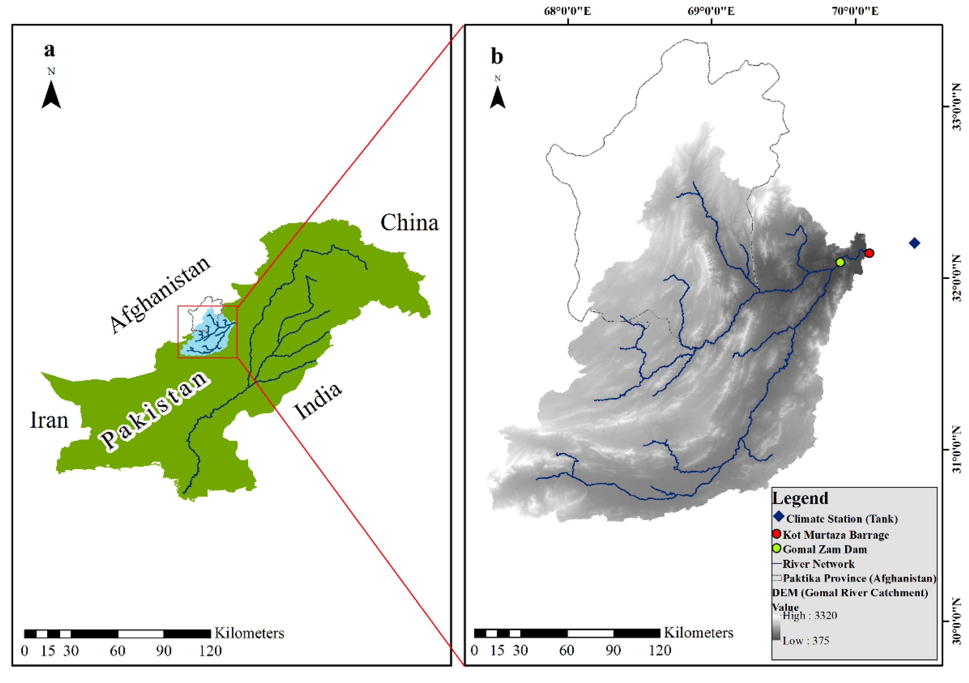
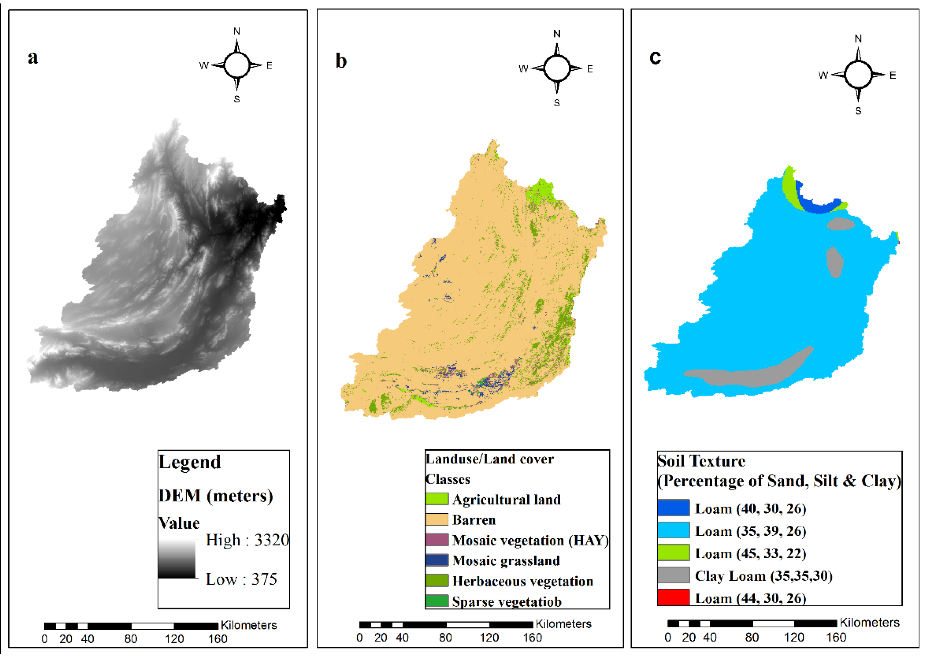
2.1. Study Area

Gomal River catchment was selected for the study to simulate the runoff and sediment yield (Figure 1). Gomal River is among the three transboundary rivers shared by Pakistan and Afghanistan that receive heavy sediment load during rainfall events due to the high soil erosion rates in the catchment. The Gomal River is the smallest among these three in terms of average annual inflow, but it is an essential source of water supply and irrigation for the downstream users in the Khyber Pakhtunkhwa (KP) province of Pakistan. The dam has a storage capacity of 1.41 BCM and started its operation in 2013.

The Gomal River originates from the mountains of Paktika province of Afghanistan and is about four hundred kilometers in length. The Gomal River catchment area at Kot Murtaza Barrage is about 36,000 km²; about 70% of the area lies within Pakistan, and 30% in Afghanistan. The elevation for the catchment ranges from 375–3320 m above the mean sea level. The average flow of Gomal River is about 0.974 Gm³ year^–1 (4.1%). According to Tank weather station data for the period 2003 to 2009, the catchment area of Gomal River receives an annual rainfall of 301 mm and minimum-maximum temperature ranges from −6 °C to 49.4 °C, respectively. The physical infrastructures in the Gomal River catchment on the Pakistan side are: (1) a storage dam with two powerhouses having a total power generation of about 91 GWh, (2) a diversion barrage, and (3) a canal irrigation system to irrigate more than 77 thousand ha of agricultural land to irrigate D.I Khan and Tank districts. A multipurpose Gomal Zam Dam was constructed on Gomal River in South Waziristan, KPK and a barrage at a 40 km downstream dam site near Kot Murtaza village.

2.2. Hydro-Meteorological Data

In this study, meteorological data of both observed and gridded precipitation products were obtained from WAPDA and online resources, respectively. Observed daily rainfall and maximum and minimum temperature data from 2003 to 2009 at the weather station in the Tank district, Pakistan, having latitude 35.183 and longitude 70.383, were obtained from the surface water hydrology project WAPDA. Daily gridded precipitation data from Global Precipitation Climatology Center (GPCC), Tropical Rainfall Measuring Mission (TRMM–3B42RT-V7), and National Centers for Environmental Prediction’s Climate Forecast System Reanalysis (NCEP-CFSR) were downloaded from the relevant websites for the period from 2002 to 2009 (http://gpcc.dwd.de/, https://globalweather.tamu.edu/, and https://giovanni.gsfc.nasa.gov/giovanni/) (

Table 1. Description of gridded precipitation datasets.

Sr. No	Gridded Precipitation Product	Spatial Resolution (Degree)	Source
1	NCEP-CFSR	0.31	(https://globalweather.tamu.edu/, accessed on 7 December 2020)
2	GPCC	1.00	(http://gpcc.dwd.de/, accessed on 12 November 2020)
3	TRMM	0.25	(https://giovanni.gsfc.nasa.gov, accessed on 1–4 December 2020)

).

The validation of gridded precipitation products requires comparison with the observed rain gauge data or use of a hydrological model and assessment of the product’s ability to predict stream flows. Both methods were used to validate the gridded datasets; however, the latter is presented in detail due to the scope of this study.

Generally, observed hydrological and sediment data are required for the calibration and validation of simulated results. Therefore, monthly observed flows and annual sediment data of the gauging station at Kot Murtaza (2004–2009) were collected from the surface water hydrology project WAPDA.

For the assessment of sediment load from the catchment and the sub-basins level, a physical-based Soil and Water Assessment Tool (SWAT) was used. The SWAT model requires Digital Elevation Model (DEM), soil type, land use, and climate datasets as inputs. The 30 m SRTM (Shuttle Radar Topography Mission) DEM was downloaded from the United States Geological Survey (USGS) (https://earthexplorer.usgs.gov, accessed on 7 April 2020). Figure 2a shows the DEM of the Gomal River catchment. The catchment boundary, stream network, and drainage pattern of the Gomal River catchment were delineated at Kot Murtaza Barrage (latitude 32.15° and longitude 70.40°). Flow direction, flow accumulation, and slope classes were obtained using the DEM (

Table 2. Slope distribution in the Gomal River catchment.

No.	Slope%	Area (ha)	% Area Coverage
1	0–20	2,252,565	65.67
2	21–40	738,221	21.52
3	41–60	303,365	8.84
4	61–80	98,472	2.87
5	>80	37,290	1.09
Total			100

). Moreover, other spatial data such as land use land cover (LULC) of the 300 m resolution were obtained from the ESA Centre for Earth Observation Rome Italy (http://due.esrin.esa.int/page_globcover.php, 15 June 2020), which distinguishes ten land use land cover classes (Figure 2b). Soil data were downloaded from the soil database of the Food and Agriculture Organization (FAO) (https://www.fao.org, accessed on 23 May 2019). According to FAO, five major soil types were identified for the study area (Figure 2c,

Table 3. Land use and soil type of study area.

Land Use Type	LU/LC (%)	Soil Texture (% Sand, Silt, Clay)	Area for Each Soil Type (%)
Agricultural land	2.08	Loam (40, 30, 26)	1.46
Barren	88.61	Loam (35, 39, 26)	88.83
		Loam (45, 33, 22)	1.70
		Clay-Loam (35,35,30)	8.00
		Loam (44, 30, 26)	0.01
Mosaic Vegetation	1.74
Mosaic grassland	0.97
Herbaceous vegetation	6.38
Sparce vegetation	0.21

).

2.3. Methods

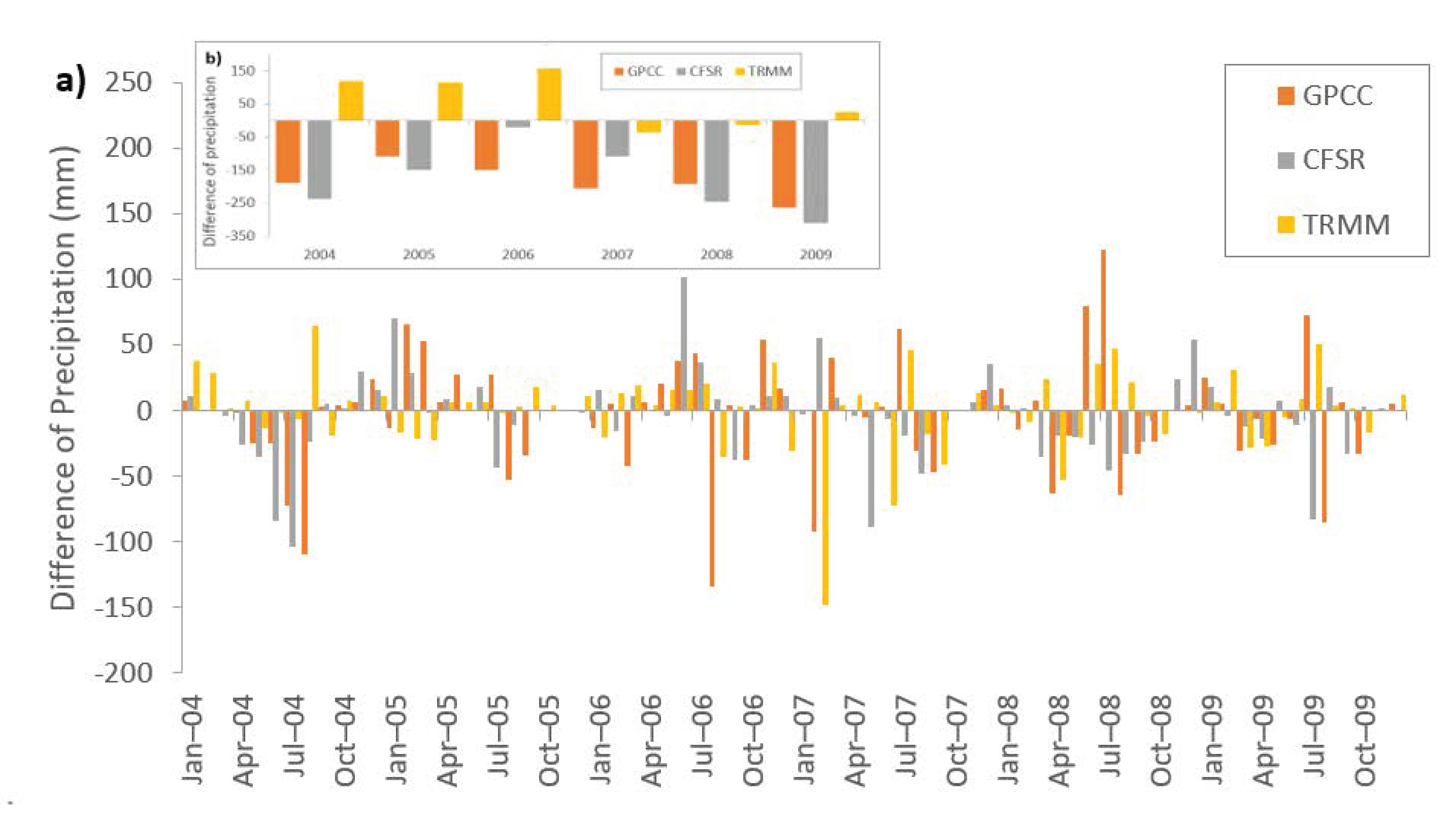
2.3.1. Precipitation Analysis

For the validation of gridded precipitation at the gauging location, the daily data were used to compute the monthly and annual precipitation. The variation of the gridded precipitation from the gauge’s precipitation data was then analyzed. Different indices were used to compare the observed and gridded precipitation datasets, including Mean Bias Error (MBE), Mean Absolute Error (MAE) and Index of Agreement (IA). The proposed indices help in assessing the accuracy of the precipitation data at a point scale. The proposed analysis was an integral part of the study; therefore, limited details are provided in this paper. However, details of the different statistical indices can be found in previous literature [14,30,31].

2.3.2. SWAT Model Setup

The first step in the model setup is the delineation of the basin area, which requires DEM as an input. The delineation process generates drainage network, flow accumulation and flow direction files. Hydrologic response units (HRUs) were delineated in the following steps.

• Reclassification of land use and soil type maps was carried out by importing these datasets into Arc SWAT.
• Five slope classes were selected, and land use and soil maps were overlaid with these slopes to finalize HRUs.
• A total of 220 HRUs and 32 sub-basins were defined for the selected catchment.

The SWAT model simulates the hydrological cycle by employing the water balance equation (Equation (1)).

$${\mathrm{SW}}_{\mathrm{t}}={\mathrm{SW}}_{\mathrm{o}}+{\displaystyle \sum }_{\mathrm{i}=1}^{\mathrm{t}}\left({\mathrm{R}}_{\mathrm{day}}-{\mathrm{Q}}_{\mathrm{surf}}-{\mathrm{E}}_{\mathrm{a}}-{\mathrm{W}}_{\mathrm{seep}}-{\mathrm{Q}}_{\mathrm{gw}}\right)\mathrm{i}$$

(1)

where ${\mathrm{SW}}_{\mathrm{t}}$depicts the final soil water content (mm); ${\mathrm{SW}}_{\mathrm{o}}$is the initial soil water content (mm); t denotes time (days); R_day is the amount of precipitation on day i (mm); Q_surf is the amount of surface runoff on day i (mm); E_a is the amount of evapotranspiration on day i (mm); W_seep is the amount of water entering the vadose level zone from the soil profile on day i (mm); and Q_gw shows the amount of return flow on day i (mm).

The estimation of surface runoff and peak runoff rates in SWAT was simulated using daily rainfall data in all HRUs. The SWAT model uses the SCS curve number method and the Green & Ampt infiltration method to estimate and simulate surface runoff. The precision of the Green & Ampt method is better than the other option due to its accuracy. However, it requires more detailed rainfall data (i.e., subset (sub-daily time step data), thus making its application complicated. Since the study area is data scarce, we employed the SCS curve number (CN) method to overcome this issue and to provide reliable results in the data-scarce watershed.

The peak discharge or the peak surface runoff rate (${\mathrm{Q}}_{\mathrm{peak}})$ was calculated with a modified rational method. The sediment loss can be predicted on the basis of the peak runoff rate, because the greater the runoff rate, the greater the erosive power of the flow.

The potential evaporation was calculated using the Hargreaves method due to its simple input parameters, i.e., daily minimum and maximum air temperature.

The sediment yield in the SWAT model was estimated using the Modified Universal Soil Loss Equation (MUSLE) (Equation (2)).

$$\mathrm{Sed}=11.8\left({\mathrm{Q}}_{\mathrm{surf}}{\ast \mathrm{Q}}_{\mathrm{peak}}{\ast \mathrm{Area}}_{\mathrm{hru}}\right)0.56{ \mathrm{K}}_{\mathrm{usle}}{ \mathrm{C}}_{\mathrm{usle} }{\mathrm{P}}_{\mathrm{usle}}{ \mathrm{LS}}_{\mathrm{usle}} \mathrm{CFRG}$$

(2)

where Sed is the sediment yield in metric tons/ha, Q_surf is the surface runoff volume in millimeters, Q_peak is the peak runoff rate in cubic meters per second, Area_hru is the area of HRU in hectares, K is the soil erodibility factor, LS is the slope factor, C is the Crop cover factor, P is the erosion control practice factor, and CFRG is the coarse fragment factor.

SWAT requires climate data as primary input data for the simulation of hydrological processes. These available climate data were prepared in text (.txt) format and imported into the SWAT model, and the SWAT input tables were populated using the model window. The model was run for seven years from 2003 to 2009 using the precipitation gauge data, including one year for warmup, and for gridded precipitation datasets (i.e., GPCC, NCEP-CFSR, and TRMM), the model was run from 2002 to 2009, with two years of warmup period/equilibrium period, as suggested by [32].

The SWAT model performance was assessed by selecting the indicators as suggested by [30,31,33,34]. For flows, three approaches or statistical indices were selected and used to determine the performance of the model, i.e., coefficient of determination (R²), Nash–Sutcliffe efficiency (NSE) and percentage bias (PBIAS). Meanwhile, the model performance for the sediment yield estimations was assessed using R² and NSE. The criteria proposed by [35] were used to judge the model simulations that indicates the satisfactory performance if NSE > 0.5 and PBIAS = ±25% for flow and NSE > 0.5 and PBIAS = ±55% for sediment. The same criteria were used for this study; details of the performance indicators can be found in [36].

2.3.3. Model Calibration

The automatic model calibration was performed on a monthly basis for three (3) years from 2004 to 2006 based on the selected parameters with their initial values, as mentioned in

Table 4. List of selected parameters for runoff and sediment yield.

Variable	Parameters Name	Description
Flow	CN2	Curve number
	SOL_AWC	Available water capacity of the soil layer
	SOL_K	Saturated hydraulic conductivity of soil
	RCHRG_DP	Deep aquifer percolation fraction
	ALPHA_BF	Base flow alpha-factor (days)
	ESCO	Soil evaporation compensation factor
	SURLAG	Surface runoff lag time
	CH_N2	Manning’s “n” value for the main channel
	SLSUBBSN	Average slope length
Sediment	SPEXP	Exponent parameter for calculating sediment re-entrained in channel sediment routing
	SPCON	Linear parameter for calculating the maximum amount of sediment that can be re-entrained during channel sediment routing
	USLE_K	Universal soil loss equation soil erodibility factor
	USLE_C	Universal soil loss equation land cover factor,
	USLE_P	Universal soil loss equation practice factor
	CH_COV1	Channel erodibility factor
	CH_COV2	Channel cover factor
	CN2	Curve number

. The SUFI-2 algorithm of SWAT-CUP was used for this purpose. The value of NSE > 0.5 was selected as an objective function to model the results. Similarly, validation was carried out from 2007 to 2009, which involved the use of the calibrated model without making any further adjustments in the values of parameters that were fitted during the calibration process, as suggested by [37].

Firstly, the simulations were performed to calibrate the runoff based on the selected parameters as shown in Table 4. For the study area, parameters were selected based on the previous literature and the physical features of the study area, such as steep slope and barren land [1,31,38,39,40,41,42,43].

3. Results and Discussion

3.1. Precipitation Analysis

A graph of the differences between the selected precipitation datasets (i.e., TRMM, GPCC and CFSR) and the gauge data is shown in Figure 3. The TRMM data show the best agreement among all the gridded precipitation datasets used for the study on a monthly basis, and the values of MBE, MAE, and IA were calculated as 0.35, 18.36 and 0.80, respectively. On an annual basis, TRMM and CFSR underestimated the precipitation throughout the study period. However, estimates of TRMM precipitation improved after 2006. Overall, TRMM precipitation was overestimated by about 1%, whereas the GPCC and CFSR presented 13 and 15% underestimations of precipitation, respectively, when compared with the observed data of the precipitation gauge for the study period. These results corroborate the previous findings for catchments in other regions of the world [44,45].

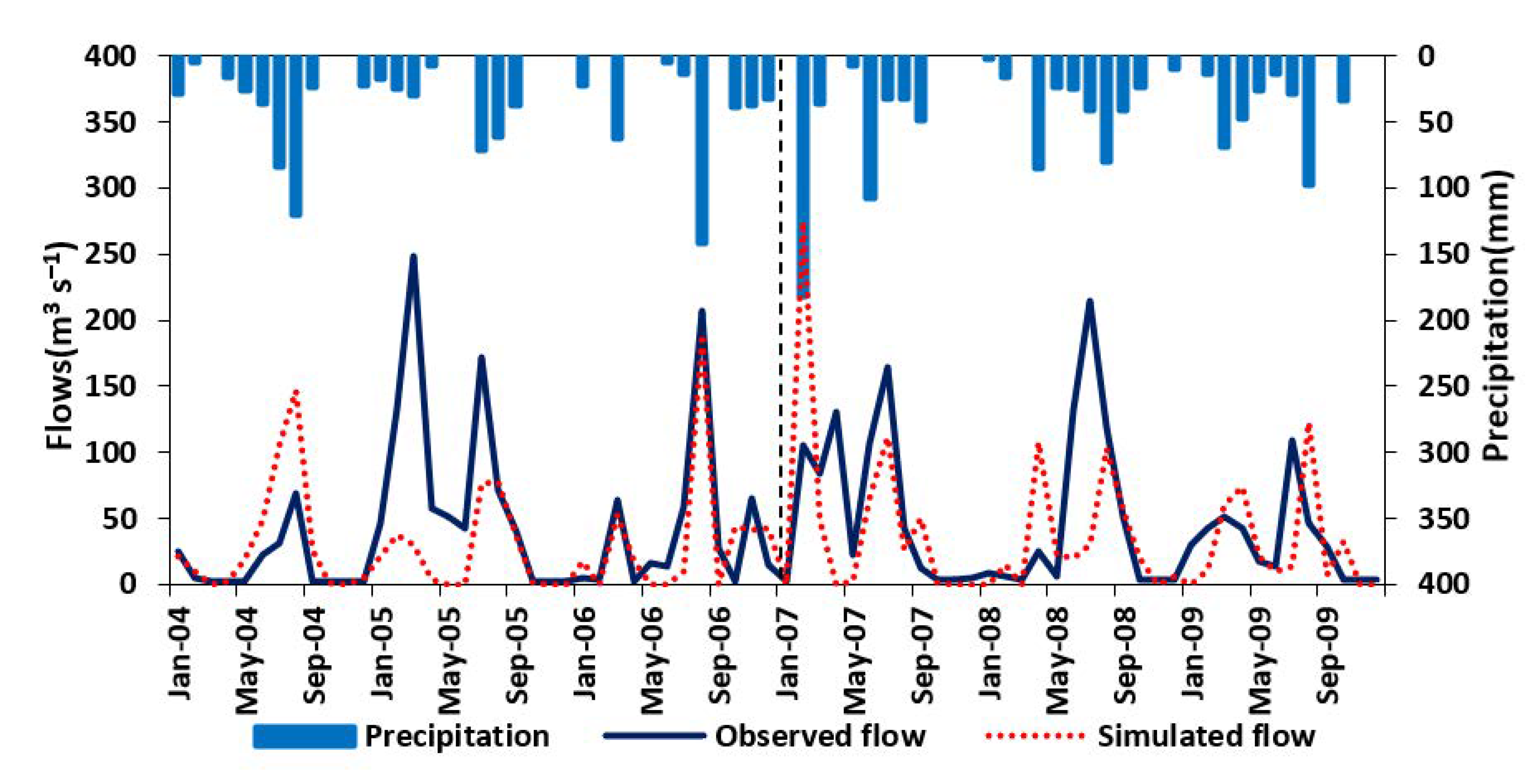
3.2. Runoff Simulations

Firstly, the runoff calibration was performed based on the selected parameters as discussed in the Methods section. The final selected parameters for runoff and sediment calibration with their initial absolute ranges and fitted values are listed in

Table 5. List of the selected parameters and their ranges.

Parameter Name	Variable	Parameter Initial Range		Fitted Values with Observed Precipitation	Fitted Values with GPCC	Fitted Values with TRMM	Fitted Values with CFSR
		Min	Max
CN2	Flow	35	98	58.8	67.5	46	87
SOL_AWC		0	1	1.38	0.85	1.04	0.85
SOL_K		0	2000	167.1	262.7	194.8	190.0
RCHRG_DP		0	1	0.13	0.00	0.07	0.21
ALPHA_BF		0	1	0.24	0.33	0.29	0.25
ESCO		0	1	0.86	0.65	0.66	1.01
SURLAG		0.05	24	19.2	20.7	18.4	22.7
CH_N2		−0.01	0.3	0.13	0.29	0.18	0.22
SLSUBBSN		10	150	94.7	90.7	60.3	24.1
SPEXP	Sediment	1	1.5	1.3	1.5
SPCON		0.0001	0.01	0.01	0.01
USLE_K		0.25	0.40	0.32	0.38
USLE_C		0.40	1.0	0.72	0.95
USLE_P		0	1	0.96	0.97
CH_COV1		−0.05	0.6	0.22	0.03
CH_COV2		−0.001	1	0.50	0.64
CN2		35	98	58.3	97.4

. The fitted parameter values for the observed and GPCC datasets showed the closest agreement. However, the model-fitted parameter values (e.g., CN2, SOL_AWC, and SOL_K) for the GPCC precipitation dataset were slightly greater than those in the observed precipitation dataset, indicating a greater runoff contribution from the surface and sub-surface as compared with the observed precipitation. Similarly, for the sediment estimations, the GPCC precipitation dataset presented higher fitted values of soil erodibility (USLE_K), practice management factor (USLE-P), and the cover management factor (USLE_C) compared to the observed precipitation dataset, which corroborates the previous findings [5]. A single value of USLE_C was assumed, because the study area is the source area for generating runoff and sediment load, and no significant seasonal variation occurs in vegetation due to the unavailability of irrigation facilities. Similarly, the value of USLE_K factor was bounded between 0.25 and 0.40, because a very limited range of soil classes prevails in the study area. Moreover, the CFRG factor was assumed to be 1 on the basis of observations during the visit to the study area, as the course fragment in the catchment was found at very limited locations. The parameter ranges selected for the flow and sediment simulations using the observed and GPCC precipitation datasets are given in Table 5. Moreover, the ranges of fitted parameters for flow simulations using TRMM and CFSR are also mentioned.

The fitted parameters for simulated flows using the gauge and GPCC precipitation datasets have slightly different values, which supports the findings of [29], who reported that the SWAT model calibrated individually with different precipitation datasets presented the lowest uncertainty in the simulated flows.

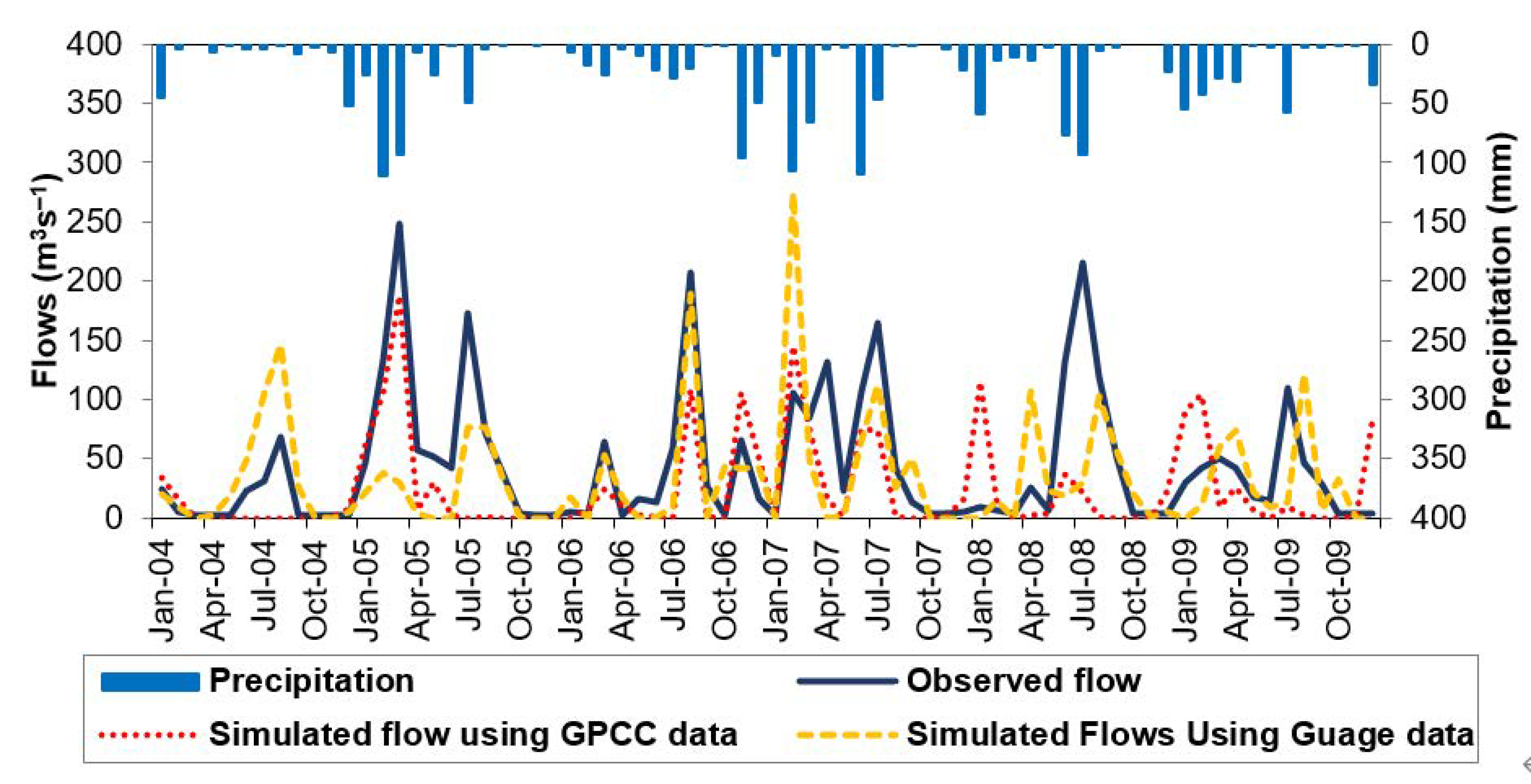
3.2.1. Runoff Estimations Using Observed Precipitation Dataset

The runoff estimations were calibrated against the monthly flows from 2004 to 2006 and validated from 2007 to 2009 at Kot Murtaza Bridge (Figure 4). The runoff computations were based on a single rain gauge site, i.e., at Tank, near the catchment outlet, due to the unavailability of precipitation data within the catchment. Despite the data limitations, the model simulated the runoff satisfactorily during most months. The differences between the simulated and observed flow can be attributed to the spatial distribution of precipitation in the catchment. Overall, the observed flows were greater than the simulated ones. For the calibration period, the observed flows were lower for several months, i.e., during August 2004 and February 2007. During Summer (June 2004 to September 2004), the simulated flows were higher than the observed ones, and rainfall during these months varied from 35 mm to 120 mm. Similarly, from January 2005 to August 2005, the simulated runoff was lower than the observed one; however, the rainfall during this period varied from 0 to 70 mm. Overall, the results indicate that the model responds to rainfall events fairly, but did not show good agreement with observed flows. The higher runoff estimation during the low flow months (November to April) could be attributed to the contribution from the base flow, i.e., snowmelt in the upper catchment areas. However, the actual snow-fed area and its contribution in Gomal River is unknown.

The value of coefficient of determination (R²) for monthly stream flow at Kot Murtaza was 0.31. Similarly, the Nash–Sutcliffe efficiency (NSE) and percentage bias (PBIAS) were found to be 0.24 and 28.9%, respectively. The values of R², NSE, and PBIAS showed the average performance of SWAT model. During the validation period, the model performance was not good enough based on the value of coefficient of determination (R²), which was calculated as 0.16, while Nash–Sutcliffe efficiency (NSE) and percentage bias (PBIAS) were −0.22 and 20.7%, respectively. Similarly, the negative value of NSE shows that the mean observed flows were more reliable than the simulated flows [35]. While the positive PBIAS indicates the underestimation of the simulated stream flows as compared to the observed one, it was nevertheless closer to the upper limit of the satisfactory criteria (i.e., ± 15%) during the validation period. Moreover, during the validation period, the simulated peak flow was much higher in February 2007 and April 2008 compared to the observed one, but when considering the rainfall during that particular month, the model shows a good response. The other reason for the low performance of the model could be the errors in the flow measurement because of the unrest conditions and the remoteness of the area during the selected study period. Moreover, the very steep river slope and the boulders in the river bed may have caused errors in stream cross-section calculation, and velocity and depth of flow measurements. Most probably, the number of precipitation stations has a significant impact on the simulation of flow in the SWAT model, and its efficiency decreases with decreasing number of precipitation stations [46]. Therefore, the use of single station rainfall data led to inaccurate simulation of high, medium and low flows. To overcome this limitation, we investigated the impact of gridded precipitation datasets on runoff and sediment load predictions, as discussed in the following sections.

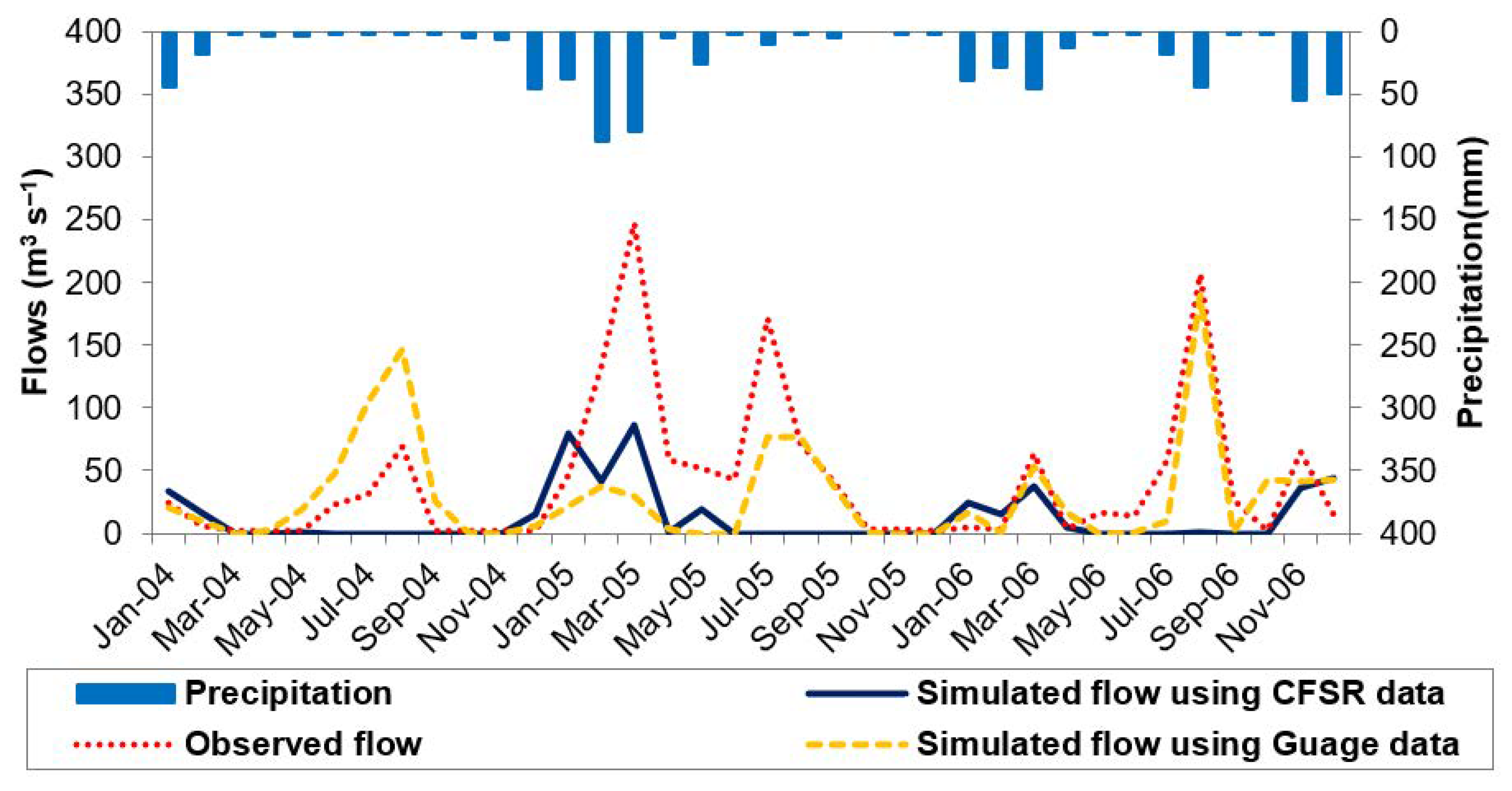
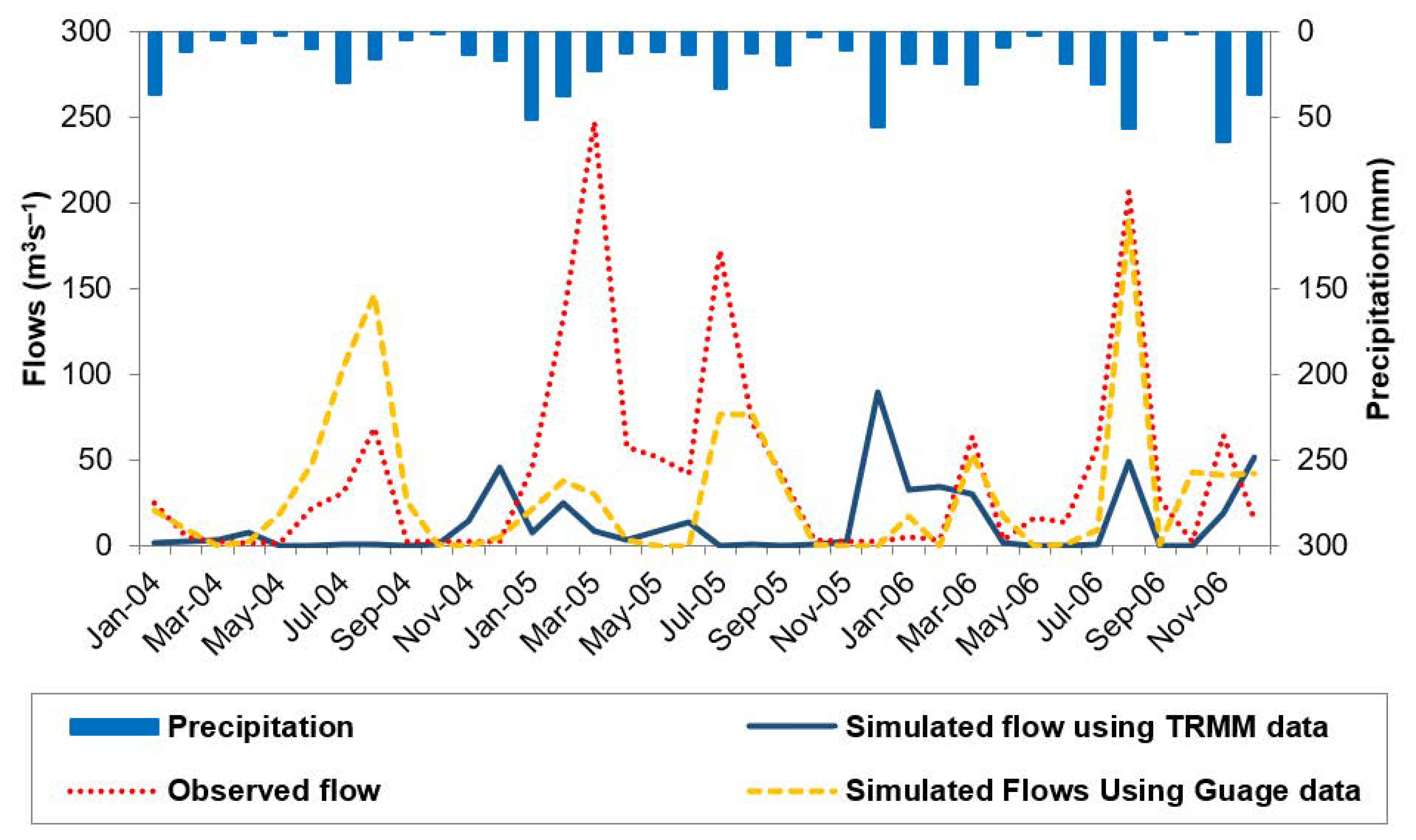
3.2.2. Runoff Computations Using Gridded Data Precipitation Datasets

The precipitation gauge is located in a plain several kilometers from the Gomal catchment stream gauging site, i.e., near Kot Murtaza, as opposed to the hilly terrain of the catchment from which the runoff originates. Therefore, runoff was not accurately estimated, as indicated by the low values of the performance indicators (see Section 3.2.1). Moreover, the single value for precipitation gauge data is not representative for such a large catchment due to the spatial distribution nature of the precipitation. Therefore, considering these limitations, three gridded precipitation datasets (i.e., GPCC, CFSR and TRMM) were used to assess the runoff from the Gomal River catchment. As discussed in the previous section, runoff from the catchment was simulated on a monthly basis. The simulated runoff during the calibration and validation period using the GPCC gridded dataset is shown in Figure 5.

During the calibration period (2004–2006), the values of statistical indices, i.e., coefficient of determination (R²), Nash–Sutcliffe Efficiency (NSE), and Percentage bias (PBIAS) were 0.56, 0.43 and 49.7%, respectively. The values of statistical indices showed that model runoff simulations were not in good agreement with the observed flow. The high PBIAS value indicated that the model-simulated runoff values were greatly underestimated during the calibration period. Moreover, during January 2005 to March 2005, the simulated and observed flows were very close, while simulated runoff was much lower during April to October in 2004 and 2005, and higher in December 2006 compared to the observed one (Figure 5).

During the validation period (2007–2009), the values of R², NSE and PBIAS were 0.08, −0.25 and 42.4, respectively, which indicated the poor performance of the model during the validation period. Moreover, the negative value of NSE indicates that the mean observed flows are more efficient than the simulated flows. Figure 5 shows that the model responds to individual rainfall events reasonably, but in July 2008 and 2009, the simulated flow was much lower than the observed one; however, rainfall during that particular month was 93 and 58 mm, respectively.

Similarly, the runoff simulations were carried out using the CFSR and TRMM precipitation gridded datasets (Figure 6 and Figure 7). However, the results were not encouraging. The CFSR dataset presented values of R², NSE and PBIAS of 0.17, 0.09 and 70.1%, respectively, which shows very poor prediction ability for runoff and indicates that the CFSR dataset is inefficient for simulating the stream flows in the Gomal River catchment. Moreover, the greater value of PBIAS indicates a significant underestimation of simulated runoff during the calibration period. Similarly, for the TRMM dataset, the values of R², NSE and PBIAS were calculated as 0, −0.32 and 69.9, respectively, during calibration (Figure 7). The calibration results showed that TRMM and CFSR precipitation datasets were not efficient for simulating the runoff in the Gomal River catchment; therefore, further validation processes were not carried out.

The value of the coefficient of determination (R²) is over-sensitive to extreme flows [47]. Similarly, the low R² or zero values indicate that the model was not able to successfully compute the extreme or peak flows. Furthermore, negative NSE indicates the goodness of the mean observed flows as compared to the simulated flows. Similarly, the greater value of PBIAS indicates the underestimation of simulated runoff during the calibration period. However, GPCC precipitation dataset performed well among the selected gridded products. The underestimation of runoff during the warmer months should be further investigated, and a suitable evapotranspiration method should be proposed for the arid and barren catchment areas. Studies on the Upper Indus Basin (UIB) have revealed that the use of observed precipitation records also presented low values of NSE (−0.43) and PBIAS (72.87%) for the sub-basins of River Indus [18]. Similarly, using the CFSR precipitation datasets with the 18 existing stations demonstrated improved performance in hydrological models [19]. However, both catchments are either snow-fed or in combination with glacier-fed river flows.

The results of the study support the findings of [21], where greater runoff generation was reported using station data at lower elevations than when using gridded precipitation datasets, because gridded precipitation estimates were on the higher side compared to the station data. However, this statement was true only for the TRMM data in our case, which predicted more precipitation during most of this time. Meanwhile, the other two precipitation datasets (CFSR and GPCC) showed less precipitation compared to the station at low elevation. This inconsistency can be attributed to the precipitation system (i.e., monsoon), which nourishes the area at which the low-elevation station is installed. Moreover, despite there being more precipitation at low elevations, runoff generation was lower than the observed value, which could be attributed to spatial variation in precipitation due to different precipitation systems, which nourish the area and cause climatic variations in such large catchments.

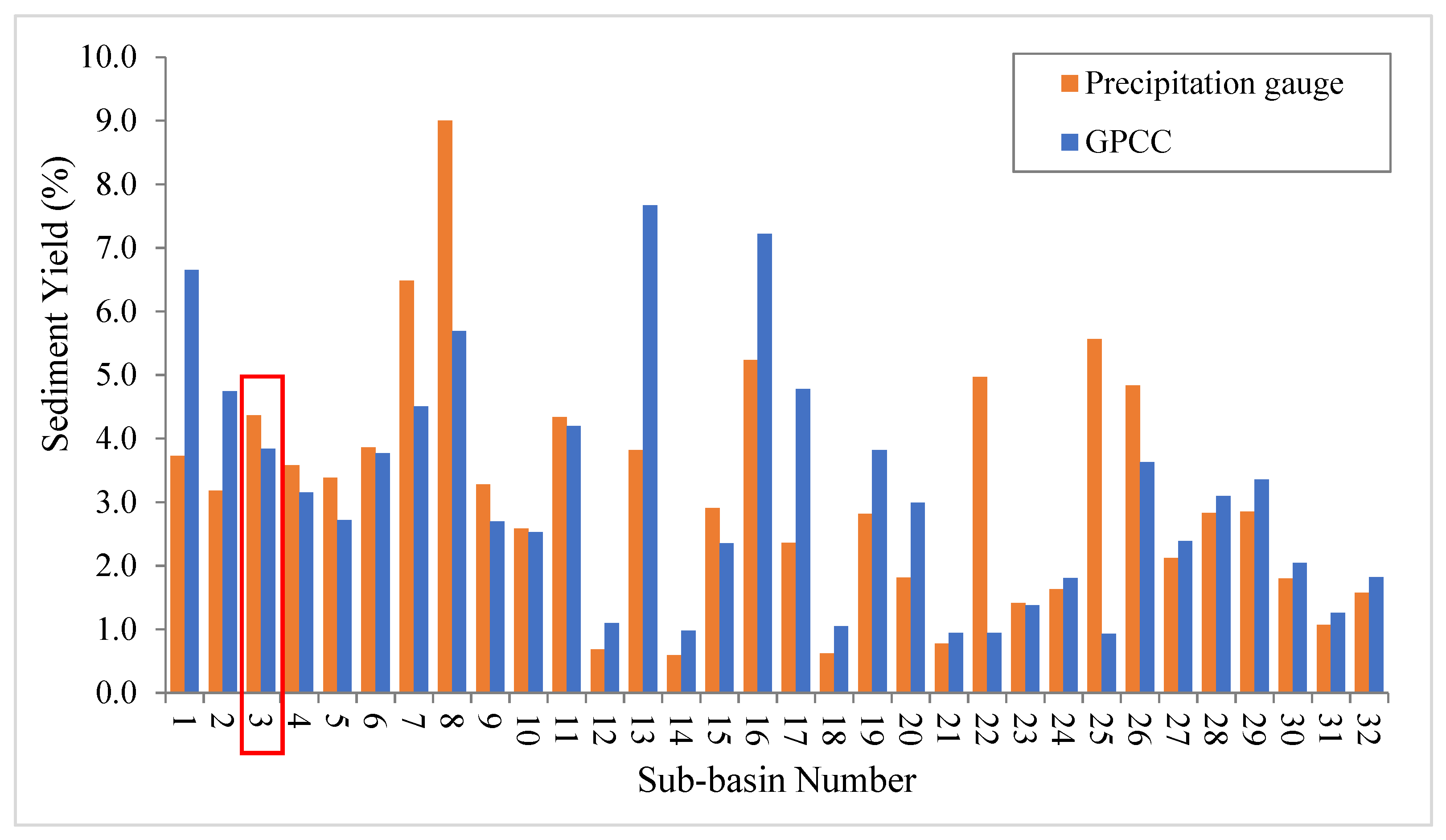
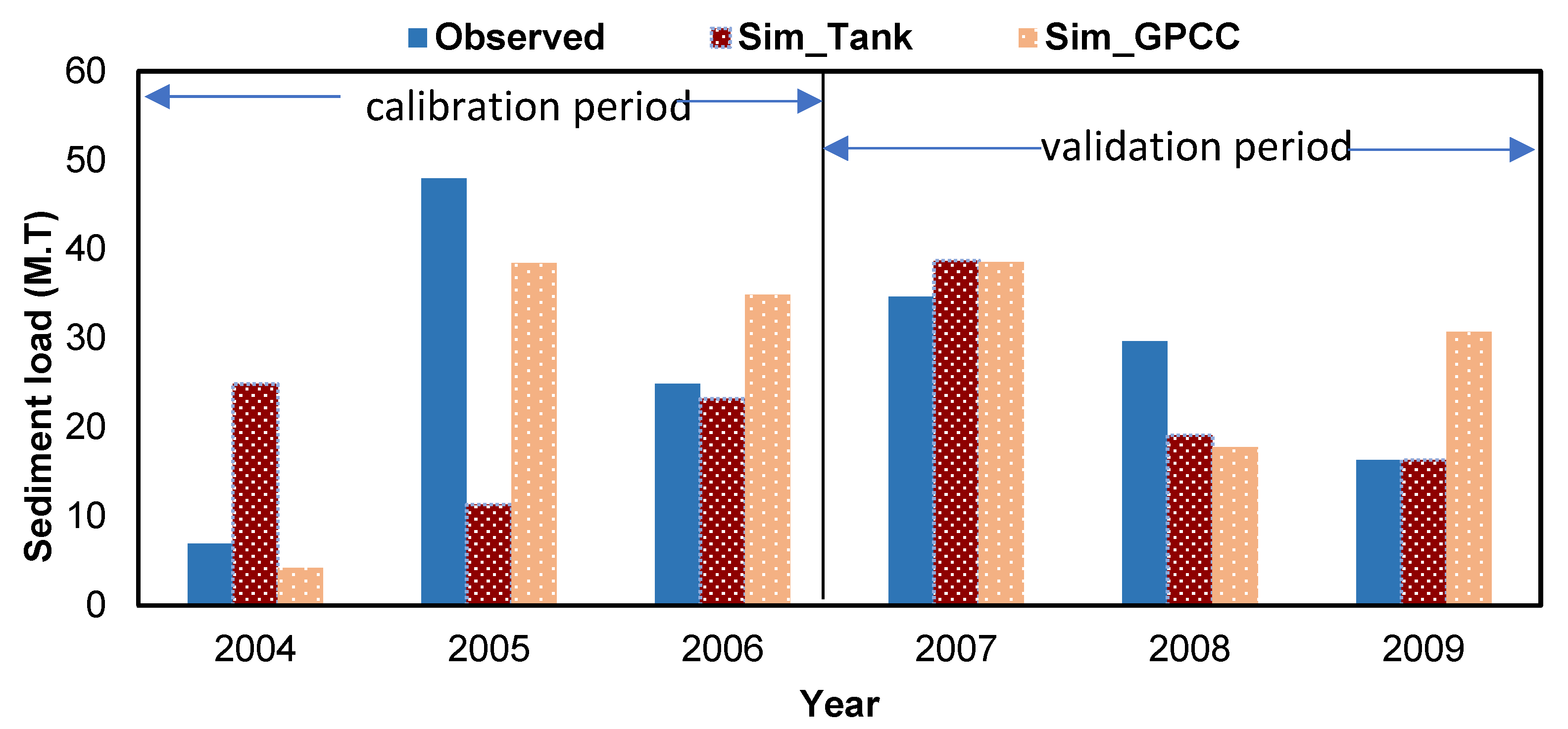
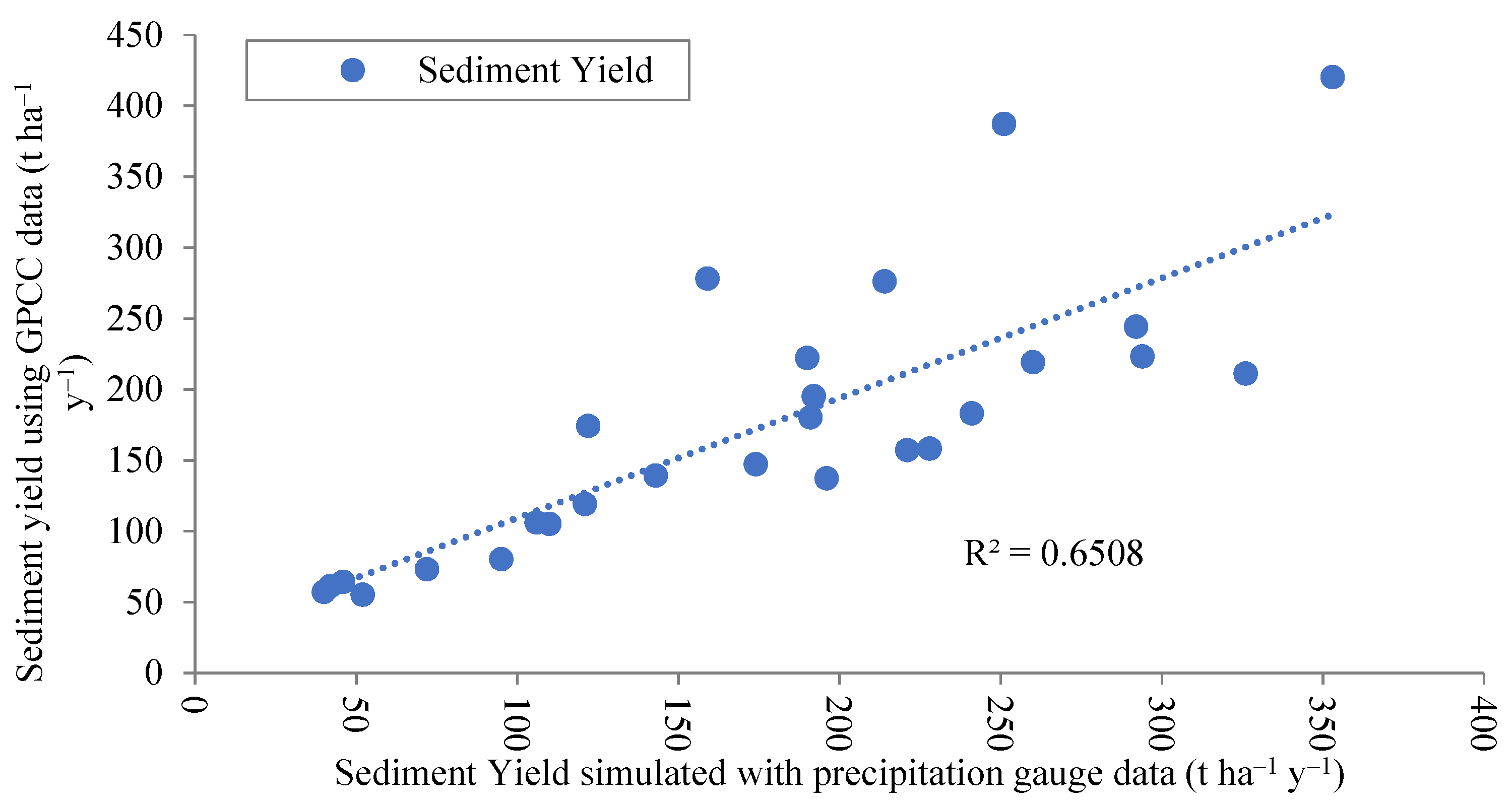
3.3. Sediment Yield Estimations

The precipitation gauge data at the Tank station and the GPCC gridded datasets provided comparatively better runoff estimations. Therefore, the same datasets were used for the calibration and validation of the SWAT model for sediment yield estimations. Sediment yield was estimated on an annual basis at the Kot Murtaza barrage site. The model was calibrated and validated for sediment yield for the periods 2004–2006 and 2007–2009, respectively (Figure 8).

The simulated sediment yield using the precipitation gauge data was close to the computed one for the years 2006, 2007 and 2009. For the observed precipitation, the coefficient of determination (R²) and Nash–Sutcliffe efficiency (NSE) were calculated as 0.89 and −0.97, respectively, during the calibration period. The higher value of R² (i.e., 0.89) indicated the better performance of the SWAT model for sediment yield estimation. The negative value of NSE was due to over and underestimations of the annual sediment load during 2004 and 2005, respectively. This indicates that the observed sediment loads for 2004 and 2005 are more efficient than the simulated ones. However, the computed sediment yield in 2006 was in very close agreement with the observed sediments, i.e., −6.7%. The computed sediment yield for the validation period (2007–2009) possessed a better value of NSE, i.e., 0.28. The differences between observed and simulated sediment loads for the years 2007, 2008 and 2009 were 11.83, −35.6 and 0.1%, respectively.

The values of R² (0.77) and NSE (0.77) for the GPCC precipitation dataset also indicate the good performance of the model for determining the annual sediment load during the calibration period. The differences between the observed and simulated sediment during the calibration period were −39.3, −19.9 and 40.3%, respectively. In 2005, the computed sediment load was in close agreement with the observed sediment load, having the minimum variation (i.e., ≈19%). The model results for the sediment load were not satisfactory during the validation period. The percentage variations between the observed and simulated sediment load for the years 2007, 2008 and 2009 were 11.3, −40.1 and 88.2%, respectively. However, GPCC provided a better estimation of sediment yield during the study period, i.e., an overestimation of only 3%.

The sediment simulation with the precipitation gauge data revealed that the SWAT model could be used for the accurate estimation of sediment load if the flows are predicted to be close to the observed values. Ref. [14] reported that GPCC could be used as an alternate climate data source in data-scare regions such as the arid and semi-arid regions of Pakistan. Similarly, in the current study, the GPCC dataset performed better than TRMM and CFSR for simulating the runoff and sediment load for the Gomal River catchment, where the climate is arid to semi-arid. However, the GPCC dataset overestimated the sediment load in some years, which supports the findings of [48], who reported the overestimation of sediment load even following the calibration of model parameters for sediment load using SWAT-CUP. Moreover, the percentage variation between observed and simulated annual sediment load was from 258 to 76% and 88 to −40% when using the gauge and GPCC precipitation datasets, respectively.

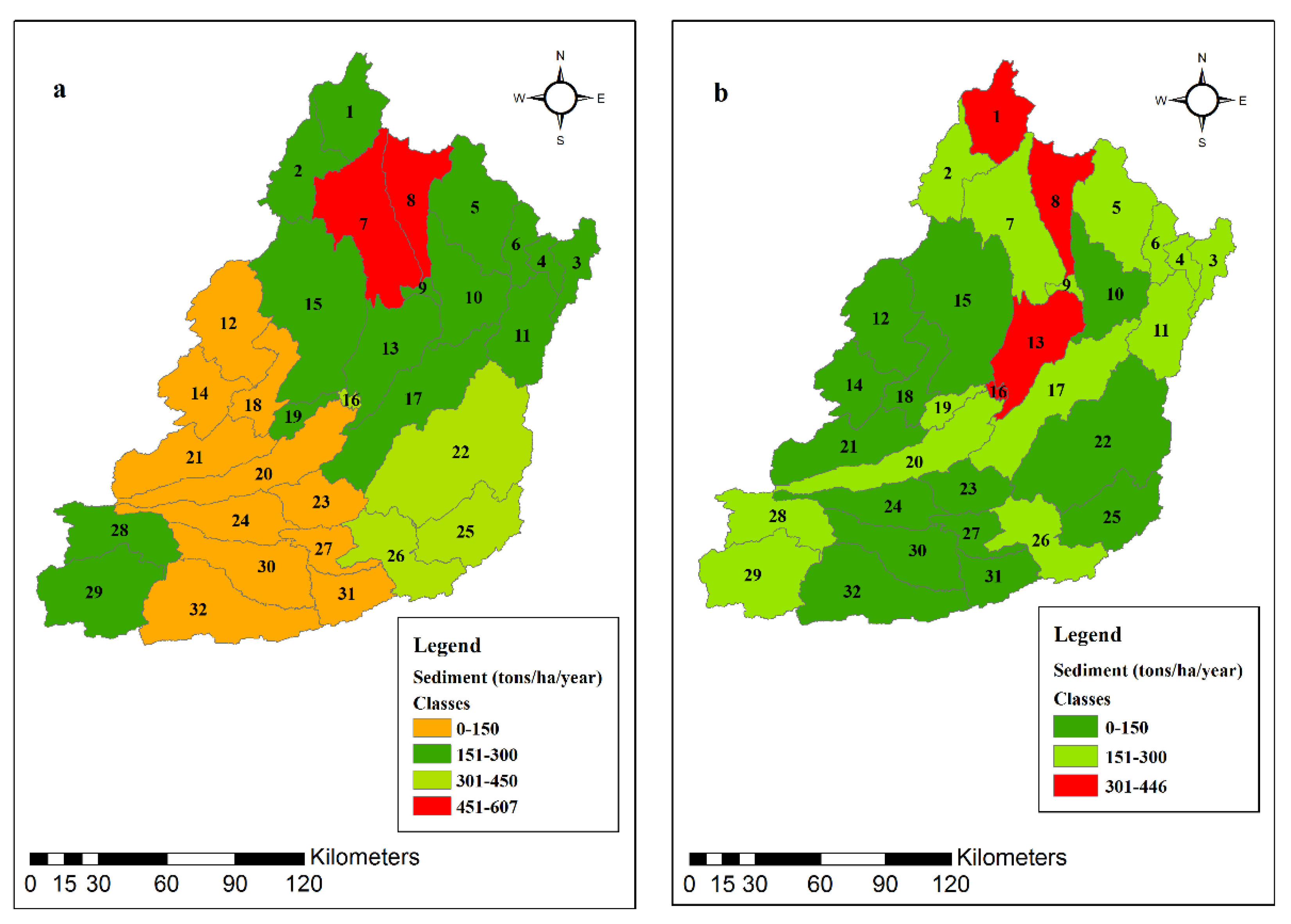
3.4. Spatial Distribution of Sediment

The spatial variability in annual sediment yield was identified for each sub-basin in the catchment based on both the observed and GPCC precipitation datasets. Identification of erosion-prone areas (sub-basins) in the catchment enables the modeler to identify the critical areas for sediment yield. Therefore, for catchment management and planning, the estimation of the spatial variations in soil erosion is beneficial. The SWAT model is the most appropriate tool for identifying sediment-prone areas at the level of HRU and subbasin in order to see which area produces the maximum and which area produces the minimum sediment.

The spatial variation in annual sediment yields in the Gomal River catchment with both precipitation inputs is shown in Figure 8. The sediment yields of different sub-basins of the Gomal River range from 40 to 607 tons ha^–1year^–1. The high sediment yield could be attributed to the prevailing catchment characteristics such as steep slope, i.e., ranges from 375 m to 3320 m with 88% barren land of the catchment, as suggested by [5,49].

The sub-basins in the northern (7, 8) and south-eastern regions (22, 25, and 26) are most susceptible to soil erosion, having an annual sediment yield of more than 300 tons ha^–1 year^–1. Moreover, the sub-basins in the south-western regions (i.e., 12, 14, 18, 21, 23, and 31) experience less erosion, having an annual sediment generation of less than 100 tons ha^–1 year^–1. Figure 9a shows that sub-basin 8 is the most vulnerable to erosion and produces maximum annual sediment yield (607 tons ha^–1 year^–1). The minimum sediment yield (40 tons ha^–1 year^–1) is generated in sub-basin 14.

Figure 9b shows the spatial distribution of sediment using the GPCC dataset and indicates that the most sensitive sub-basins possessing the maximum annual sediment generation are sub-basins 1, 8, 13, and 16. All of these sub-basins contribute annual sediment yields of more than 331 tons ha^–1. Moreover, sub-basins 12, 14, 18, 21, 22, 23, 25, and 31 contribute sediment yield of less than 100 tons ha^–1 year^–1. Sub-basin 13 is the most vulnerable, possessing an annual sediment yield of 446 tons ha^–1 year^–1, while the lowest amount of sediment is produced in sub-basin 25, which has an annual sediment yield of 54 tons ha^–1 year^–1. Overall, the GPCC precipitation dataset generated a higher sediment load for the sub-basins in the central and the southern regions of the catchment, whereas a lower sediment load was produced in the north-eastern regions.

In a recent study by [5], the soil erosion rates from the sub-basin between GZD and the barrage, i.e., sub-basin 3, were estimated, and it was reported that 15% of the sediment load still reaches the Kot Murtaza Barrage after the Gomal Zam Dam construction. Meanwhile, the contribution of sediment load from sub-basin 3 is unknown. The results of this study reveal that a significant sediment contribution (≈11%) originates from the flushing operation of the dam, because sub-basin 3 contributes only 3.8–4.5% (Figure 10). However, this small proportion of total sediment yield (≈260 t ha⁻¹ y⁻¹) contributes significantly to the total sediment yield, and is about 3 times greater than its corresponding area.

The sub-basins contributing significant sediment load can be controlled using check dams, which could be an effective control measure [10,50], because establishing vegetation is not an effective measure for these types of catchments [5]. Moreover, check dams in the sediment-producing area could reduce sediment load from 64 to 78 percent [51,52]. As the study area is characterized as barren, having steep slopes where vegetation establishment is almost impossible, check dams could be an effective solution for sediment management and should be constructed in the sub-basins vulnerable to erosion in the Gomal River catchment.

Sediment yield simulations at the sub-basin level using the observed and GPCC precipitation datasets show a good agreement when excluding a few sub-basins (i.e., 7, 8, 13, 22, and 25), which make up 23% of the total area (Figure 11). Therefore, there is great potential for the use of GPCC precipitation data in ungauged or data-scarce regions.

4. Conclusions and Recommendations

Runoff and sediment yield for the data-scarce Gomal River catchment (i.e., a transboundary river) were predicted using the SWAT model. Precipitation gauge data and three gridded precipitation products, i.e., GPCC, CFSR and TRMM-3B42RT, were used as input for the SWAT model for runoff and sediment yield assessment at the Kot Murtaza Barrage on Gomal River. The spatial distribution of sediment yield was also assessed in order to evaluate the sediment load contribution from each sub-basin. The specific conclusions of the study are as follows:

Analysis of gridded precipitation datasets shows that the TRMM resulted in the highest accuracy (i.e., ≈1%) compared with the total precipitation of the gauge during the selected period. However, runoff computations by the SWAT model using the input precipitation of the gauge and GPCC datasets were better than with TRMM and CFSR. Moreover, the underestimation of runoff highlights the role of precipitation stations at higher elevations in the catchment and the need for further improvements in the GPCC dataset, respectively.

The sediment yield simulated using GPCC data was in good agreement with the computed sediment yield at the stream gauging station. However, the GPCC precipitation dataset overestimated sediment yield compared with the predicted one using precipitation data of the gauge. This fact emphasizes the improvements in the method for measuring sediment concentration data and the use of an appropriate sediment load computation approach like a continuous record that requires data on a daily basis. The annual sediment load predicted by the SWAT model using GPCC follows an almost similar trend to that of the observed values. However, underestimation of the runoff during summer should be investigated further. The relationship of the sediment yields simulated using the precipitation gauge and the GPCC datasets resulted in a good correlation (R² = 0.65) at a sub-basin scale. However, the GPCC precipitation results showed a higher sediment yield for the sub-basins in the central and the southern part of the catchment, while a lower sediment yield was found in the north-eastern part compared with the gauge precipitation input. Therefore, additional precipitation gauges on the central and northern sides are able to enhance the accuracy of the simulated runoff and sediment yield. Moreover, the combined use of observed and gridded data could be the focus of future studies with the aim of improving the daily runoff and sediment load predictions using SWAT model.

The significant sediment yield (4.1% of the total) originating from the sub-basin between the GZD and the barrage (i.e., sub-basin 3) reveals that the sub-basin has an important role in contributing sediment load at the barrage site. However, a major contribution still derives from the flushing outlets of the Gomal Zam Dam when compared with the previous findings by [5]. Moreover, check dams construction at the critical sub-basins producing the highest amount of annual sediment yield could be effective control measures and help to enhance the reservoir life.

The findings of the current study encourage the application of the GPCC precipitation dataset for deciding the management of water resources and sediment load in arid to semi-arid regions with scarce precipitation data. The observed flows and sediment yield data used for this study were of a relatively shorter duration, because the measured rainfall data were available for a limited period from a single precipitation gauge only. Therefore, data of a relatively longer period could enhance the performance of the SWAT model in similar climatic regions. The accuracy and resolution of land use land cover and soil maps may influence sediment yield computations at a local scale (i.e., at the sub-basin or HRU level).

References

1. Hussain, F.; Nabi, G.; Wu, R.S.; Hussain, B.; Abbas, T. Parameter evaluation for soil erosion estimation on small watersheds using SWAT model. Int. J. Agric. Biol. Eng. 2019, 12, 96–108. [Google Scholar] [CrossRef] [Green Version]
2. Haq, I.U.L. Sediment Management of Tarbela Reservoir. Paper No. 733. 72nd Annu. Sess. Pakistan Eng. Congr. 2012. Available online: https://pecongress.org.pk/images/upload/books/2-Dr.%20Izhar%20ul%20Haq.pdf (accessed on 18 April 2022).
3. Ahmad, M.-u.-D.; Peña-Arancibia, J.L.; Yu, Y.; Stewart, J.P.; Podger, G.M.; Kirby, J.M. Climate change and reservoir sedimentation implications for irrigated agriculture in the Indus Basin Irrigation System in Pakistan. J. Hydrol. 2021, 603, 126967. [Google Scholar] [CrossRef]
4. Borrelli, P.; Robinson, D.A.; Fleischer, L.R.; Lugato, E.; Ballabio, C.; Alewell, C.; Meusburger, K.; Modugno, S.; Schütt, B.; Ferro, V.; et al. An assessment of the global impact of 21st century land use change on soil erosion. Nat. Commun. 2017, 8, 2013. [Google Scholar] [CrossRef] [Green Version]
5. Bhatti, M.T.; Ashraf, M.; Anwar, A.A. Soil erosion and sediment load management strategies for sustainable irrigation in arid regions. Sustainability 2021, 13, 3547. [Google Scholar] [CrossRef]
6. Aghsaei, H.; Mobarghaee Dinan, N.; Moridi, A.; Asadolahi, Z.; Delavar, M.; Fohrer, N.; Wagner, P.D. Effects of dynamic land use/land cover change on water resources and sediment yield in the Anzali wetland catchment, Gilan, Iran. Sci. Total Environ. 2020, 712, 136449. [Google Scholar] [CrossRef]
7. Li, B.; Li, C.; Liu, J.; Zhang, Q.; Duan, L. Decreased streamflow in the Yellow River basin, China: Climate change or human-induced? Water 2017, 9, 116. [Google Scholar] [CrossRef]
8. Abebe, T.; Gebremariam, B. Modeling runoff and sediment yield of Kesem dam watershed, Awash basin, Ethiopia. SN Appl. Sci. 2019, 1, 446. [Google Scholar] [CrossRef] [Green Version]
9. Dutta, S.; Sen, D. Application of SWAT model for predicting soil erosion and sediment yield. Sustain. Water Resour. Manag. 2018, 4, 447–468. [Google Scholar] [CrossRef]
10. Samad, N.; Chauhdry, M.H.; Ashraf, M.; Saleem, M.; Hamid, Q.; Babar, U.; Tariq, H.; Farid, M.S. Sediment yield assessment and identification of check dam sites for Rawal Dam catchment. Arab. J. Geosci. 2016, 9, 1–14. [Google Scholar] [CrossRef]
11. Miralles, D.G.; Jiménez, C.; Jung, M.; Michel, D.; Ershadi, A.; Mccabe, M.F.; Hirschi, M.; Martens, B.; Dolman, A.J.; Fisher, J.B.; et al. The WACMOS-ET project—Part 2: Evaluation of global terrestrial evaporation data sets. Hydrol. Earth Syst. Sci. 2016, 20, 823–842. [Google Scholar] [CrossRef] [Green Version]
12. Beck, H.E.; Vergopolan, N.; Pan, M.; Levizzani, V.; van Dijk, A.I.J.M.; Weedon, G.P.; Brocca, L.; Pappenberger, F.; Huffman, G.J.; Wood, E.F. Global-scale evaluation of 22 precipitation datasets using gauge observations and hydrological modeling. Adv. Glob. Chang. Res. 2020, 69, 625–653. [Google Scholar] [CrossRef]
13. Faiz, M.A.; Zhang, Y.; Baig, F.; Wrzesiński, D.; Naz, F. Identification and inter-comparison of appropriate long-term precipitation datasets using decision tree model and statistical matrix over China. Int. J. Climatol. 2021, 41, 5003–5021. [Google Scholar] [CrossRef]
14. Ahmed, K.; Shahid, S.; Wang, X.; Nawaz, N.; Najeebullah, K. Evaluation of gridded precipitation datasets over arid regions of Pakistan. Water 2019, 11, 210. [Google Scholar] [CrossRef] [Green Version]
15. Try, S.; Tanaka, S.; Tanaka, K.; Sayama, T.; Oeurng, C.; Uk, S.; Takara, K.; Hu, M.; Han, D. Comparison of gridded precipitation datasets for rainfall-runoff and inundation modeling in the Mekong River Basin. PLoS ONE 2020, 15, e226814. [Google Scholar] [CrossRef] [Green Version]
16. Jiang, S.; Zhang, Z.; Huang, Y.; Chen, X.; Chen, S. Evaluating the TRMM Multisatellite Precipitation Analysis for Extreme Precipitation and Streamflow in Ganjiang River Basin, China. Adv. Meteorol. 2017, 2017, 2902493. [Google Scholar] [CrossRef]
17. Zhang, L.; Meng, X.; Wang, H.; Yang, M.; Cai, S. Investigate the applicability of CMADS and CFSR reanalysis in Northeast China. Water 2020, 12, 996. [Google Scholar] [CrossRef] [Green Version]
18. Khan, A.J.; Koch, M. Correction and informed regionalization of precipitation data in a high mountainous region (Upper Indus Basin) and its effect on SWAT-modelled discharge. Water 2018, 10, 1557. [Google Scholar] [CrossRef] [Green Version]
19. Babur, M.; Babel, M.S.; Shrestha, S.; Kawasaki, A.; Tripathi, N.K. Assessment of climate change impact on reservoir inflows using multi climate-models under RCPs-the case of Mangla Dam in Pakistan. Water 2016, 8, 389. [Google Scholar] [CrossRef] [Green Version]
20. Yang, Y.; Wang, G.; Wang, L.; Yu, J.; Xu, Z. Evaluation of gridded precipitation data for driving SWAT model in area upstream of three gorges reservoir. PLoS ONE 2014, 9, e112725. [Google Scholar] [CrossRef]
21. Daneshvar, F.; Frankenberger, J.R.; Bowling, L.C.; Cherkauer, K.A.; Moraes, A.G.d.L. Development of Strategy for SWAT Hydrologic Modeling in Data-Scarce Regions of Peru. J. Hydrol. Eng. 2021, 26, 05021016. [Google Scholar] [CrossRef]
22. Zambrano-Bigiarini, M.; Nauditt, A.; Birkel, C.; Verbist, K.; Ribbe, L. Temporal and spatial evaluation of satellite-based rainfall estimates across the complex topographical and climatic gradients of Chile. Hydrol. Earth Syst. Sci. 2017, 21, 1295–1320. [Google Scholar] [CrossRef] [Green Version]
23. Khan, M.S.; Liaqat, U.W.; Baik, J.; Choi, M. Stand-alone uncertainty characterization of GLEAM, GLDAS and MOD16 evapotranspiration products using an extended triple collocation approach. Agric. For. Meteorol. 2018, 252, 256–268. [Google Scholar] [CrossRef]
24. Zandler, H.; Haag, I.; Samimi, C. Evaluation needs and temporal performance differences of gridded precipitation products in peripheral mountain regions. Sci. Rep. 2019, 9, 15118. [Google Scholar] [CrossRef] [Green Version]
25. Sun, Q.; Miao, C.; Duan, Q.; Ashouri, H.; Sorooshian, S.; Hsu, K.L. A Review of Global Precipitation Data Sets: Data Sources, Estimation, and Intercomparisons. Rev. Geophys. 2018, 56, 79–107. [Google Scholar] [CrossRef] [Green Version]
26. Herold, N.; Behrangi, A.; Alexander, L.V. Large uncertainties in observed daily precipitation extremes over land. J. Geophys. Res. 2017, 122, 668–681. [Google Scholar] [CrossRef]
27. Baez-Villanueva, O.M.; Zambrano-Bigiarini, M.; Beck, H.E.; McNamara, I.; Ribbe, L.; Nauditt, A.; Birkel, C.; Verbist, K.; Giraldo-Osorio, J.D.; Xuan Thinh, N. RF-MEP: A novel Random Forest method for merging gridded precipitation products and ground-based measurements. Remote Sens. Environ. 2020, 239, 111606. [Google Scholar] [CrossRef]
28. Abushandi, E.H.; Merkel, B.J. Application of IHACRES rainfall-runoff model to the wadi Dhuliel arid catchment, Jordan. J. Water Clim. Chang. 2011, 2, 56–71. [Google Scholar] [CrossRef]
29. Ajaaj, A.A.; Mishra, A.K.; Khan, A.A. Evaluation of Satellite and Gauge-Based Precipitation Products through Hydrologic Simulation in Tigris River Basin under Data-Scarce Environment. J. Hydrol. Eng. 2019, 24, 05018033. [Google Scholar] [CrossRef]
30. Haider, H.; Zaman, M.; Liu, S.; Saifullah, M.; Usman, M.; Chauhdary, J.N.; Anjum, M.N.; Waseem, M. Appraisal of climate change and its impact on water resources of pakistan: A case study of mangla watershed. Atmosphere 2020, 11, 1071. [Google Scholar] [CrossRef]
31. Rafiei, V.; Ghahramani, A.; An-Vo, D.A.; Mushtaq, S. Modelling hydrological processes and identifying soil erosion sources in a tropical catchment of the great barrier reef using SWAT. Water 2020, 12, 2179. [Google Scholar] [CrossRef]
32. Moriasi, D.N.; Gitau, M.W.; Pai, N.; Daggupati, P. Hydrologic and water quality models: Performance measures and evaluation criteria. Trans. ASABE 2015, 58, 1763–1785. [Google Scholar] [CrossRef] [Green Version]
33. Ang, R.; Oeurng, C. Simulating streamflow in an ungauged catchment of Tonlesap Lake Basin in Cambodia using Soil and Water Assessment Tool (SWAT) model. Water Sci. 2018, 32, 89–101. [Google Scholar] [CrossRef] [Green Version]
34. Musie, M.; Sen, S.; Srivastava, P. Comparison and evaluation of gridded precipitation datasets for streamflow simulation in data scarce watersheds of Ethiopia. J. Hydrol. 2019, 579, 124168. [Google Scholar] [CrossRef]
35. Moriasi, D.N.; Arnold, J.G.; Van Liew, M.W.; Bingner, R.L.; Harmel, R.D.; Veith, T.L. Model evaluation guidelines for systematic quantification of accuracy in watershed simulations. Trans. ASABE 2007, 50, 885–900. [Google Scholar] [CrossRef]
36. Betrie, G.D.; Mohamed, Y.A.; Van Griensven, A.; Srinivasan, R. Sediment management modelling in the Blue Nile Basin using SWAT model. Hydrol. Earth Syst. Sci. 2011, 15, 807–818. [Google Scholar] [CrossRef] [Green Version]
37. Refsgaard, J.C. Parameterisation, calibration and validation of distributed hydrological models. J. Hydrol. 1997, 198, 69–97. [Google Scholar] [CrossRef]
38. Abbaspour, K.C.; Yang, J.; Maximov, I.; Siber, R.; Bogner, K.; Mieleitner, J.; Zobrist, J.; Srinivasan, R. Modelling hydrology and water quality in the pre-alpine/alpine Thur watershed using SWAT. J. Hydrol. 2007, 333, 413–430. [Google Scholar] [CrossRef]
39. Arnold, J.G.; Moriasi, D.N.; Gassman, P.W.; Abbaspour, K.C.; White, M.J.; Srinivasan, R.; Santhi, C.; Harmel, R.D.; Van Griensven, A.; Van Liew, M.W.; et al. SWAT: Model use, calibration, and validation. Trans. ASABE 2012, 55, 1491–1508. [Google Scholar] [CrossRef]
40. Briak, H.; Moussadek, R.; Aboumaria, K.; Mrabet, R. Assessing sediment yield in Kalaya gauged watershed (Northern Morocco) using GIS and SWAT model. Int. Soil Water Conserv. Res. 2016, 4, 177–185. [Google Scholar] [CrossRef] [Green Version]
41. Markhi, A.; Laftouhi, N.; Grusson, Y.; Soulaimani, A. Assessment of potential soil erosion and sediment yield in the semi-arid N′fis basin (High Atlas, Morocco) using the SWAT model. Acta Geophys. 2019, 67, 263–272. [Google Scholar] [CrossRef]
42. Schmalz, B.; Fohrer, N. Comparing model sensitivities of different landscapes using the ecohydrological SWAT model. Adv. Geosci. 2009, 21, 91–98. [Google Scholar] [CrossRef] [Green Version]
43. Yuan, L.; Forshay, K.J. Using SWAT to evaluate streamflow and lake sediment loading in the xinjiang river basin with limited data. Water 2020, 12, 39. [Google Scholar] [CrossRef] [PubMed] [Green Version]
44. Camberlin, P.; Barraud, G.; Bigot, S.; Makanzu, F.; Maki, I.J.; Moron, V.; Pellarin, T.; Philippon, N.; Dewitte, O.; Martiny, N.; et al. Evaluation of remotely sensed rainfall products over Central Africa. Q. J. R. Meteorol. Soc. 2019, 145, 2115–2138. [Google Scholar] [CrossRef]
45. Diem, J.E.; Ryan, S.J.; Hartter, J. Satellite-based rainfall data reveal a recent drying trend in central equatorial Africa Satellite-based rainfall data reveal a recent drying trend in central equatorial Africa. Clim. Chang. 2014, 126, 263–272. [Google Scholar] [CrossRef]
46. Tan, M.L.; Yang, X. Effect of rainfall station density, distribution and missing values on SWAT outputs in tropical region. J. Hydrol. 2020, 584, 124660. [Google Scholar] [CrossRef]
47. Legates, D.R.; McCabe, G.J. Evaluating the use of “goodness-of-fit” measures in hydrologic and hydroclimatic model validation. Water Resour. Res. 1999, 35, 1–9. [Google Scholar] [CrossRef]
48. Lu, C.M.; Chiang, L.C. Assessment of sediment transport functions with the modified SWAT-Twn model for a taiwanese small mountainous watershed. Water 2019, 11, 1749. [Google Scholar] [CrossRef] [Green Version]
49. Koirala, P.; Thakuri, S.; Joshi, S.; Chauhan, R. Estimation of Soil Erosion in Nepal using a RUSLE modeling and geospatial tool. Geosciences 2019, 9, 147. [Google Scholar] [CrossRef] [Green Version]
50. Zhao, G.; Kondolf, G.M.; Mu, X.; Han, M.; He, Z.; Rubin, Z.; Wang, F.; Gao, P.; Sun, W. Sediment yield reduction associated with land use changes and check dams in a catchment of the Loess Plateau, China. Catena 2017, 148, 126–137. [Google Scholar] [CrossRef]
51. Li, E.; Mu, X.; Zhao, G.; Gao, P.; Sun, W. Effects of check dams on runoff and sediment load in a semi-arid river basin of the Yellow River. Stoch. Environ. Res. Risk Assess. 2017, 31, 1791–1803. [Google Scholar] [CrossRef]
52. Mishra, A.; Froebrich, J.; Gassman, P.W. Evaluation of the SWAT model for assessing sediment control structures in a small watershed in india. Trans. ASABE 2007, 50, 469–477. [Google Scholar] [CrossRef]
Figure 1. Map of Gomal Zam River catchment at Kot Murtaza Barrage: (a) Gomal River catchment sharing Pakistan and Afghanistan, (b) Gomal River catchment, GZD site, stream and precipitation gauging sites.
Water 14 01480 g001
Figure 2. Spatial data inputs: (a) DEM, (b) land use land cover, (c) soil texture classes (percentages of silt sand and clay are given in parentheses).
Water 14 01480 g002
Figure 3. Difference between gridded precipitation and gauge data: (a) on a monthly basis, (b) on an annual basis.
Water 14 01480 g003
Figure 4. Simulated and observed hydrograph on monthly basis using precipitation gauge data for the calibration (2004–2006) and validation (2007–2009) periods.
Water 14 01480 g004
Figure 5. Simulated and observed hydrograph on monthly basis using GPCC dataset.
Water 14 01480 g005
Figure 6. Runoff simulations using CFSR dataset.
Water 14 01480 g006
Figure 7. Runoff simulation using TRMM dataset.
Water 14 01480 g007
Figure 8. Simulated and observed sediment on an annual basis using the Tank and GPCC datasets.
Water 14 01480 g008
Figure 9. Spatial distribution of sediment yield in the Gomal River catchment: (a) tank rainfall station dataset; (b) GPCC gridded dataset.
Water 14 01480 g009
Figure 10. Sediment yield (as percentage of total) from each sub-basin using observed precipitation and the GPCC dataset.
Water 14 01480 g010
Figure 11. Relationship between sediment yields simulated with observed and GPCC precipitation datasets.
Water 14 01480 g011