Abstract
Climate change is driving worsening flood events worldwide. In this study, a hybrid approach based on a combination of the optimization of a hydrodynamic model and an error correction modeling that exploit different aspects of the physical system is proposed to improve the forecasting accuracy of flood water levels. In the parameter optimization procedure for the hydrodynamic model, Manning’s roughness coefficients were estimated by considering their spatial distribution and temporal variation in unsteady flow conditions. In the following error correction procedure, the systematic errors of the optimized hydrodynamic model were captured by combining the input variable selection method using partial mutual information (PMI) and artificial neural networks (ANNs), and therefore, complementary information provided by the data was achieved. The developed ANNs were used to analyze the potential non-linear relationships between the considered state variables and simulation errors to predict systematic errors. To assess the hybrid forecasting approach (hydrodynamic model with an ANN-based error correction model), performances of the hydrodynamic model, two ANN-based water-level forecasting models (ANN1 and ANN2), and the hybrid model were compared. Regarding input candidates, ANN1 considers the historical observations only, and ANN2 considers not only the historical observations that used in ANN1 but also the prescribed boundary conditions required for the hydrodynamic forecast model. As a result, the hybrid model significantly improved the forecasting accuracy of flood water levels compared to individual models, which indicates that the hybrid model is able to take advantage of complementary strengths of both the hydrodynamic model and the ANN model. The optimization of the hydrodynamic model allowing spatially and temporally variable parameters estimated water levels with acceptable accuracy. Furthermore, the use of PMI-based input variable selection and optimized ANNs as error correction models for different sites were proven to successfully predict simulation errors in the hydrodynamic model. Hence, the parameter optimization of the hydrodynamic model coupled with error correction modeling for water level forecasting can be used to provide accurate information for flood management.
1. Introduction
Floods are one of the most severe natural disasters, and more frequent floods occur due to climate change and changes in land use [1,2,3]. River flooding can significantly disrupt important services, including energy, infrastructure, water provision, and transport [4]. Therefore, flood forecasting is a critical issue for the security of individuals and infrastructures and water resources management. An accurate flood simulation and forecasting can provide useful information for flood management and control. A flood routing model can be used to estimate potential damage in a specific reach in which a hydraulic structure may also be included.
Physically based hydraulic models are based on an understanding of the physical process that occurs within a natural system and reproduce the dominant processes through governing equations that are derived under a few simplifying assumptions. Typically, it is not possible to include each process within a simulation model owing to various simplifications and assumptions, and thus, the resulting model can only approximate a real-world system. Despite efforts focused on improving the performance of various open channel flow models, errors between the computed and corresponding observed values are inevitably obtained due to the uncertainties that arise in the model itself, hydrological boundary conditions (upstream flow or lateral inflow) and initial conditions, and model parameters (numerical parameters, geometric parameters, and hydraulic parameters) [5]. All these uncertainties simultaneously affect errors in the model output that produce fairly poor model performance despite a thorough understanding of the governing laws. Gupta et al. [6] emphasized that sophisticated methods are extremely essential to provide corrections for physically based models with respect to water control problems.
In order to provide more accurate information about flood flow, simulation errors produced during the modeling process can be corrected by using postprocessor methods. The selected error correction model should extract useful information about the physical process that was not considered during the construction of a physically based hydrodynamic model such that additionally obtained information can remove systematic biases of the calibrated hydrodynamic model. In contrast to physically based models, data-driven models are not based on either a pre-conceived conceptualization of the behavior of the system or an explicit representation of discrete physical processes [7]. Conversely, in data-driven models, system response is characterized by exploiting statistical information in a set of time-series data [8]. Furthermore, data-driven models can use the advantages of whatever relevant data are available, and this allows such models to represent particular processes [9]. The fact that data-driven models exploit the relationship between data, whereas hydrodynamic flow models are based on physical principles, gives them a complementary nature [7,10,11].
Several studies were performed to improve the river flow forecasting of rainfall runoff models by coupling a conceptual model with a data-driven error correction model [7,12,13,14,15,16,17]. Konapala et al. [10] used a machine learning algorithm known as a long short-term memory (LSTM) network to simulate the process-based hydrologic model residual. Cho and Kim [18] also employed LSTM to predict the residual errors of WRF-Hydro. The complementary modeling approach was also applied to groundwater problems [19,20,21] and reservoir water level prediction [22]. Nevertheless, there is a paucity of research attention on the use of complementary modeling approaches for hydraulic models, especially in open channel unsteady flow simulations for flood forecasting. Torres-Rua et al. [8] used data-driven models to correct errors in hydraulic simulation models for canal flow schemes in irrigation water management. Bruen and Yang [23] and Preis et al. [24] applied complementary modeling to improve the model performance for urban drainage systems and urban water networks, respectively. Abebe and Price [25] indicated that it is possible to effectively use a parallel data-driven model to predict errors in a flood routing model (a particular form of the 1D diffusive wave equation). The data-driven models used in the aforementioned studies include autoregressive, autoregressive moving average, genetic algorithm, and artificial neural networks (ANNs).
In order to improve the accuracy of flood forecasting, it is significant to integrate or hybridize a physically based hydraulic model and a data-driven model such that it is possible to extract complementary strengths and eliminate weaknesses in the respective modeling methodologies as opposed to continuing to choose between the individual techniques and employing them in isolation [9,26,27]. In this study, ANN models were conjunctively used as error correction models to complement a flood routing model based on the idea that it is possible to significantly improve the overall description of flood flow [25]. A looped network unsteady flow model was constructed for the Han River in South Korea. Unlike Ayvaz [28] who only considered the variability in roughness parameters along a flow reach, the variability in Manning’s roughness coefficient, which is related to both the discharge and the flow reach, was considered by adopting a power function as the relationship between Manning’s roughness coefficient and discharge in each sub-reach such that the characteristic of the physical process can be fully considered (hereafter, the term “Manning’s n” is used instead of “Manning’s roughness coefficient”). Specifically, ANNs were employed as error correction models in the study as this modeling approach was applied in several studies and was demonstrated as an optimal technique for developing a model of residual errors for a hydrodynamic model [25]. A nonlinear input variable selection algorithm based on the estimation of partial mutual information (PMI), which was proved as efficient and highly suited for the development of ANN models [29], was applied to ensure that appropriate state variables (that are neither under-specified nor over-specified for estimating simulation errors) are selected as model inputs. The approach integrating the hydrodynamic model and ANNs was estimated by comparing the performances of the hydrodynamic model, two ANN-based forecast models with different input sets, and the hybrid model. The goal of this study is to improve the accuracy of flood water level estimation by coupling the optimized hydrodynamic model with ANN-based error correction modeling, so that different aspects of the physical system from the two types of models are fully exploited.
2. Hydrodynamic Flow Model for the Han River
2.1. Study Area
The flow reach in the study corresponds to the 69 km between Paldang Dam and Junryu Gauging Station and is the main stream of the Han River in South Korea (Figure 1). The water levels are measured at five stations, namely, Paldang Bridge, Banpo Bridge, Hangang Bridge, Heangju Bridge, and Junryu Gauging Station (Figure 2). Two submerged weirs in the channel, namely, the Jamsil and Singok submerged weirs (Figure 1), are partially gated structures. The gates of movable weirs are fully opened during flood periods, and thus, two different flows occur at the fixed weir and movable weir.

Figure 1.
Study area: Han River.

Figure 2.
Schematic representation of the modeled river reach [30].
2.2. Hydrodynamic Flow Model
A looped-network unsteady flow model was developed for the Han River. This is owing to the unique features of the Han River with respect to the hydraulic structures in it. Governing equations for the looped-network model consist of equations for the link and the node. With respect to the links, equations are further divided into one for fluvial flow and another for weir-type flow. Governing equations for fluvial links include following continuity and momentum equations:
in which Q(x, t) denotes the discharge, h(x, t) denotes the water surface elevation, x and t denote the space and time variables, respectively, A(x, h) represents the cross-sectional area of water, K(x, h) denotes the conveyance, α denotes the energy correction factor assumed to be unity, and g denotes the gravitational acceleration. The conveyance is given as follows:
in which R denotes the hydraulic radius, and n denotes Manning’s roughness coefficient.
Governing equations for weir-type links are expressed as follows:
where s and f denote discharge coefficients, b denotes the effective width of the weir, and hw denotes the weir crest elevation. Upstream and downstream water levels are denoted as hu and hd, respectively, and Qu or Qd denotes the discharge of weir overflow.
The nodal continuity equation at any node j is expressed as follows:
where J denotes the total number of nodes, Lj denotes the total number of links connected to node j, and Qj,k denotes the discharge from node k. Qext(j, t) denotes the external inflow to the node, such as inflows from upstream boundaries or tributaries of the channel. Equal water level is assumed as a nodal energy equation as follows:
This implies that the water level hj,k for each computational point on link k is identical to the nodal water level, hj.
Equations (1) and (2) are discretized by the Preissmann’s four-point implicit scheme (e.g., [31,32]). The discretized equations in conjunction with Equations (4)–(7) constitute a nonlinear system in which stages and discharges at computational points and nodal water surface elevations are unknown. This system is solved by using the Newton–Raphson method involving the application of the looped double sweep algorithm. The general solution algorithm comprises of four phases for each iteration as follows: link forward sweep, node matrix loading, node solution, and link backward sweep. Details of the solution algorithm are reported in a study by Holly et al. [33].
2.3. Model Set Up
The Paldang Dam is the upstream boundary of the model where discharge is known. Water levels are gauged at the Paldang Bridge, Banpo Bridge, Hangang Bridge, and Jeonryu station. Observed water levels at the Paldang Bridge, Banpo Bridge, and Hangang Bridge were used for model calibration and validation, and those at the Jeonryu station were used for downstream boundary conditions. Measured tributary inflows were given as model inputs. The model consists of 10 nodes (1 at either end of the river reach, an upstream/downstream pair at each of the 2 submerged weirs, and 1 at each of the 4 tributary-inflow junction points) and 11 links (Figure 2). Nodes located upstream and downstream of the submerged weirs are connected by two links while the remaining nodes are connected by one link. There are 156 computational points, and the water levels computed at 3 sites (the Paldang, Banopo, and Hangang Bridges) were used for comparison with the corresponding observed levels.
As previously stated, the submerged weirs at Jamsil and Singok are composed of a fixed weir and a movable weir, and the gates of the movable weirs were fully opened during flood periods. Therefore, channel- and weir-type flows separately occurred on either side. In order to simulate these two flows, a fluvial- and a weir-type link were used for the channel- and weir-type flows, respectively, in the model. The two links connect the upstream and downstream nodes of submerged weirs by forming a loop (Figure 2) [30].
The initial conditions of each flood event were obtained by modeling 200 h of steady state flow. Boundary conditions at the beginning of an event were used for the inputs of the steady state flow. A steady condition was assumed to be achieved after performing 200 h of steady state flow simulation and obtained flows and water levels were used for the initial conditions of the unsteady state flow model.
3. Methodology
3.1. Basic Idea
The main procedure used in the study is described as follows:
- (1)
- Develop an unsteady flow model that allows for time-varying distributed parameters;
- (2)
- Identify model parameters by using an optimization technique;
- (3)
- Compute model errors between computed and observed data;
- (4)
- Select the variables (at corresponding lag times) that are closely related to the model errors by analyzing the relationship between the model residuals and different state variables (e.g., observed discharge and water level, previous residuals, etc.) at varying lag times by using the PMI-based input variable selection method;
- (5)
- Construct data-driven models (artificial neural networks) that estimate the residuals of the hydrodynamic model by using the best-related variables selected in the previous step;
- (6)
- Improve the outputs of the hydrodynamic model by adding the estimated errors as corrections.
Figure 3 shows the framework used in the study. The procedure shows that the hydrodynamic flow model is initially executed, and this is followed by the error correction model. The forecasts are improved by combining the results of the two models. The hydrodynamic model used in the study is the looped-network unsteady flow model that considers variable hydraulic roughness. An ANN model was used to estimate residual errors of the hydrodynamic model by considering time series that are closely related to the model errors. The PMI-based approach was used to identify optimal input variables for ANN development based on the dependence between input and output variables. The underlying hypothesis of the proposal is that the data-driven model can capture the systematic patterns presented in the residuals of the hydrodynamic model based on the learning relationship between model residuals and a few data series. It is assumed that the structural problems in the hydrodynamic model and data can be reflected in the detected patterns.
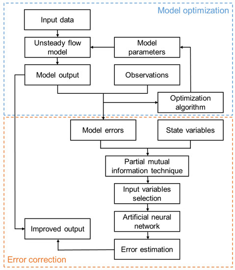
Figure 3.
The flowchart illustrating the methodology.
3.2. Parameter Identification
A hydrodynamic flow model that numerically solves Saint-Venant equations requires Manning’s roughness coefficient as a model parameter to represent flow resistance. Most previous studies only focused on a lumped-parameter model in which Manning’s n is considered as a constant value (e.g., [34,35,36]). Few studies, including Fread and Smith [37] and Ayvaz [28], consider the spatial and/or temporal variation in Manning’s n, although it is extremely significant for practical problems.
The entire flow reach was divided into two sub-reaches based on the differences in the channel characteristics of the upstream and downstream reaches of the Wangsook stream junction. The downstream reach of the Wangsook stream junction is a channelized reach, while the upstream reach is more similar to a natural river, in which the cross sections are highly irregular. A power function (Equation (8)) that describes the relationship between Manning’s n and discharge was adopted for each sub-reach (Figure 4) [30,38]. Therefore, the model has two different Manning’s n-discharge relationships for two sub-reaches that describe the variation in Manning’s n with space and discharge, i.e., n = n(x, Q(x, t)), as follows:
where I denotes the total number of sub-reaches, and denote the coefficients of the power function, and denotes Manning’s n for sub-reach i. Two power functions are used for the model, and thus it is possible to identify four parameters (, , , ) in the model calibration.
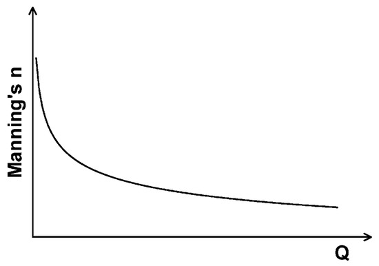
Figure 4.
Functional relationship between Manning’s n and discharge: power function [30].
The criterion used for the parameter optimization involves determining model parameters that minimize the sum of squares of the errors between computed and observed stages. The objective function is expressed as follows:
in which and denote observed and computed water levels, respectively, at time t at the k-th station, n denotes a parameter vector that represents a set of model parameters, and S denotes the sum of squares of errors between computed and observed water levels. A parameter optimization tool, PEST, that applies a Gauss–Marquardt–Levenberg algorithm, was used to estimate model parameters [39].
3.3. ANN-Based Error Correction Method
Error correction methods mainly focused on correcting the model output time-series of interest [40]. An ANN, which is a data-driven modeling approach, was used to develop an error correction model in this study to reproduce the errors of the hydrodynamic model. Therefore, the output of hydrodynamic model is modified by passing it through the ANN.
An ANN is a powerful tool to address various practical problems, and it is extensively used for simulation and forecasting in diverse areas such as water resources, power generation, finance, and environmental science [41]. Extant studies that focus on its applications in water resources include [23,42]. An ANN learns from data and their potential to accurately describe the behavior of complex nonlinear systems [23]. The ANN model used in this study involves determining the relationship between simulation errors of the hydrodynamic model and a few state variables.
An ANN consists of several layers of neurons (nodes) that are interconnected by links using weights (parameters) [23]. It processes information in a manner similar to the information processes in the human brain [43]. Specifically, ANNs are developed to represent the relationships that are inherent within the data by training the network. A network receives data through input neurons arranged in an input layer and subsequently passes it to the successive layers through a transfer or activation function such as a sigmoid or logistic curve. The flexible architectures enable ANNs to represent complex nonlinear processes without explicitly using a theoretical algorithm to describe the nonlinearity [43].
A three-layer neural network was used in the study to estimate residuals by training with the gradient-based method. The inputs of the ANN were selected in the procedure of input variable selection by using the PMI method, and the output corresponded to the modified residuals. Generally, more than one hidden layer is used for the multi-layer feedforward network. However, the use of a single hidden layer is recommended [44], and this recommendation was adopted by several studies that apply multi-layer feedforward networks in hydrology and water resources [45,46,47,48]. Hence, a hidden layer was used in this study, and the appropriate numbers of hidden neurons were determined by trial and error during the training phase. Figure 5 shows the basic structure of the ANN used in the study. Each neuron in a neural network receives and processes input from other neurons with the exception of neurons at the input layer. The weighted sum of the input data is processed in the hidden layer by using a sigmoid function in this study and is given as follows:
where denotes the input data at the i-th input neuron; denotes the output of the j-th hidden neuron; denotes the weighting value connecting and ; and L denotes the number of neurons in the input layer.
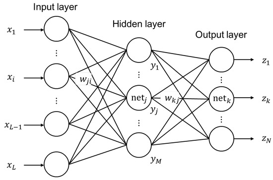
Figure 5.
Multi-layer perceptron.
The activation function in the output layer is a simple linear function that calculates the weighted sum of the hidden layer outputs that is given as follows:
where denotes the output of k-th output neuron; denotes the weighting value connecting and ; and M denotes the number of neurons in the hidden layer.
In the training phase, the Levenberg–Marquardt algorithm, which is a blend of gradient decent and Gauss–Newton iteration, was used to optimize the weights connecting neurons by minimizing the mean absolute error (MAE) between the targeted data and the estimated data from ANN. Previous ASCE studies [49,50] describe the ANN model details. The modified residuals were subsequently added to the outputs of the hydrodynamic model to obtain improved results.
3.4. PMI-Based Input Variable Selection Method
The first and an important step in ANN development involves identifying the variables that exhibit the strongest relationship with simulation errors and can replicate error behavior. Specifically, the accuracy of the artificial neural network is significantly related to effective input variables. The challenge of selecting appropriate input variables involves selecting the fewest variables that are neither over-specified nor under-specified while adequately describing the underlying input–output relationship [51].
Several input variable selection techniques were developed by ANN modelers. The two main types of input variable selection techniques include wrapper and filter algorithms. Wrapper algorithms are model-based techniques that treat the variable selection as an optimization of the model structure. A weakness of using a wrapper algorithm is the large number of potential computations for trial calibration and evaluation [52]. Furthermore, the applicability of the selected input variables obtained by using a wrapper technique is restricted because the appropriateness of selected variables for a certain model structure is not guaranteed for another structure [53]. In contrast to model-based wrapper techniques, model-free filter techniques use a statistical measure. The separation of the variable selection tasks from the model development tasks makes the technique more effective and also allows the wider applicability of the selected input set to different model architectures [54]. May et al. [54,55] presented a review of recent input variable selection methods for ANNs.
An efficient technique reduces the need for extensive trial-and error and arbitrary judgement during model development. The PMI technique is a model-free filter approach that considers inter-dependencies between candidates and deals with nonlinear modeling without the assumption of linearity. An input variable selection algorithm based on the estimation of PMI was initially introduced by Sharma [56] and further developed by Bowden et al. [29] and May et al. [54,55]. Some studies indicated that PMI-based input variable selection is a highly suitable measure for input variable selection during ANN development since the ANN development implicitly assumes non-linear relationships between variables [43,54,55,57].
Input variable selection using PMI-based algorithms can significantly reduce the amount of trial-and error during ANN model development and improve the performance of an ANN model. The PMI-based selection algorithm is briefly described as follows [43,54,55]:
- (1)
- Determine potential candidates based on previous knowledge;
- (2)
- Initialize the selected input variable set S that corresponds to a null set since no input variables are selected initially, and the candidate set C;
- (3)
- Compute the residual of output (u) and that of candidate variables (v) by subtracting relationship with currently selected inputs as follows:
Here, d denotes the dimension of X, b denotes the kernel bandwidth (or smoothing parameter), and denotes the sample covariance matrix.
The kernel bandwidth b is as follows:
where sf denotes the scaling factor that controls the degree of kernel smoothing; denotes the Gaussian reference bandwidth that is given as follows:
Harrold et al. [58] empirically determined that a bandwidth of approximately 1.5 provided stable estimates of mutual information;
- (4)
- Estimate the PMI and determine candidate that maximizes PMI as follows:
The estimator for f at a given location x is given as follows:
The kernel density estimation (KDE) that is one of non-parametric density estimation techniques were used in step (3) and (4) since it is typically considered as accurate and suitably robust [55];
- (5)
- Compute the values of the considered termination criterion.
The termination criterion is a key consideration in the input variable selection as it significantly affects computational efficiency and selection accuracy [59]. The Akaike information criterion (AIC) [60] can be used to measure the trade-off between the size of the input set and the accuracy of the regression filter [54]. The AIC is given as follows:
where o and p denote the number of observations and model parameters, respectively, and represents residuals.
During the input variable selection, the AIC initially decreases with the increase in the number of parameters due to a reduction in the residuals and reaches a minimum value. Subsequently, the AIC increases as the 2p term penalizes the selection of additional variables. Therefore, the selection procedure is terminated when the AIC reaches its minimum point;
- (6)
- Based on the values of the considered termination criterion, a decision is adopted to either select a candidate and continue or terminate the selection.
4. Results and Discussion
4.1. Parameter Identification for Hydrodynamic Model
The hourly observed data of 12 flood events at Paldang Bridge, Banpo Bridge, and Hangang Bridge were selected for the calibration and validation of the model. The peak discharges of these flood events at the upstream boundary range from 5147 m3/s to 16,146 m3/s. The flood events were numbered in the decreasing order of the peak discharge at the Paldang Dam and split into two data sets. Flood events corresponding to 1, 3, 5, 7, 9, and 11 were used for calibration, and the rest were used for model validation (Table 1).

Table 1.
Flood events used for calibration and validation of the hydrodynamic model.
The model parameters were determined by averaging the optimized parameters for each flood event in the calibration. The estimated power functions in Figure 6 that were derived by considering the geometric average of calibrated coefficients show that Manning’s n decreases when the discharge increases in both sub-reaches and that the values of Manning’s n for the upstream reach tend to be greater than those for the downstream reach given a uniform discharge. The identified power functions obtained in the calibration were used to simulate flood events corresponding to 2, 4, 6, 8, 10, and 12, as a validation procedure. The average root mean square errors (RMSEs) for calibration and validation are 0.205 and 0.308, respectively, and this indicates that the model that uses a power function as the Manning’s n–discharge relationship can estimate flood water levels with acceptable accuracy.
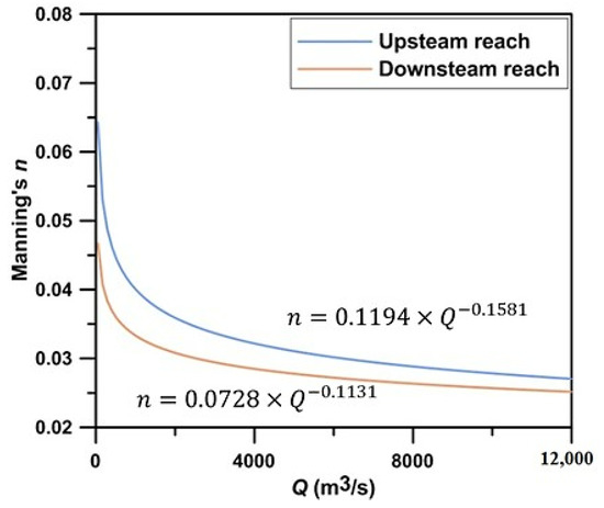
Figure 6.
Identified power functions for upstream reach and downstream reach.
4.2. Error Correction Using ANN Models
4.2.1. PMI-Based Input Variable Selection
In order to test the approach that combines the hydrodynamic model and ANNs, a performance comparison of the hydrodynamic model, ANNs, and hybrid model (hydrodynamic model with ANN-based error correction model) was carried out. An ANN model, labeled here as ANN1, was developed to forecast water levels at specific locations using historical observations as inputs. The considered input candidates and output of ANN1 are shown in Figure 7. Furthermore, an ANN model, denoted as ANN2, was constructed for water level forecasting with input candidates including not only the inputs used in ANN1 but also prescribed boundary conditions at , , …, that were required for the hydrodynamic forecast model (Figure 8). Finally, an ANN for error correction of the hydrodynamic model, labeled as ANN3, was developed with candidate inputs including the predicted boundary conditions of the hydrodynamic model, historical observations, calculated water levels by the hydrodynamic model, and recorded errors of the hydrodynamic model (Figure 9). In Figure 7, Figure 8 and Figure 9, and represent the observed and prescribed discharges at the Paldang Dam, respectively; and are the observed and prescribed tributary inflows, respectively; and are the observed and prescribed water levels at the Junryu gauge station; is the observed water level at gauging stations; HM_ is the computed water level by the hydrodynamic model; is the time derivative of the observed water level; HM_ is the time derivative of the computed water level by the hydrodynamic model; is the forecasted water level at the k-th station; and is the errors of the hydrodynamic model at the k-th station.
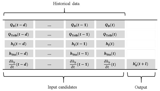
Figure 7.
Input candidates and output for ANN1.
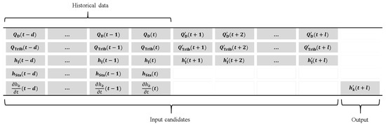
Figure 8.
Input candidates and output for ANN2.
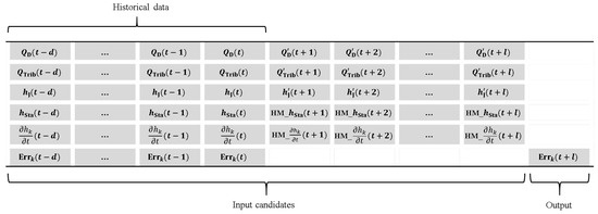
Figure 9.
Input candidates and output for ANN3.
For the considered ANNs, the number of potential inputs can be quite large, as shown in Figure 7, Figure 8 and Figure 9; however, given their correlated nature, many may be redundant. The travel time of flow from upstream boundary (Paldang Dam) to downstream boundary (Junryu gauging station) approximately corresponds to 1~2 h for most historical flood events. However, it is difficult to precisely measure the travel time from the upstream boundary to the downstream boundary owing to the tidal effect. Therefore, lagged variables from current time t to the previous 5 h (the maximum lag time d) were assumed as sufficient in the study.
The derivative of water levels can be used to describe the flow situation. For example, a zero or low derivative indicates normal or base flow while a high positive derivative indicates the rising limb of a flood event, and a high negative derivative indicates the recession limb of a flood event. Therefore, the rate of flow changed and its lagged variables were also considered as possible input variables in ANN models.
From the input candidates, input variables for ANN models were selected by applying the PMI technique. Data of 12 flood events (Table 1) were used for input variable selection using PMI. Based on the AIC criterion, input sets that satisfy were selected. The selected input variables for ANNs at different lead times and at different sites are listed in Table 2, Table 3 and Table 4. In the tables, subscribes P, B, H, and W represent the Paldang Bridge, Banpo Bridge, Hangang Bridge, and Wangsook Stream, respectively.
Table 2.
Selected input variables for ANN1.
Table 3.
Selected input variables for ANN2.
Table 4.
Selected input variables for ANN3.
Selected input variables for ANN1 show that water level forecasting at the Paldang Bridge is mainly determined by observed water levels at the Paldang Bridge, and discharges at the Paldang Dam. The inflow from the Wangsook Stream also affects the water level forecasting as the lead time increases (Table 2). Table 2 shows that 1-h lead time forecasting at the Banpo Bridge and Hangang Bridge is related to the observed water levels at four gauge stations, i.e., Paldang Bridge, Banpo Bridge, Hangang Bridge, and Junryu gauge station. Table 3 shows the selected input variables for ANN2 which considers not only historical observations but also the predicted boundary conditions used in the hydrodynamic model. The selected variables show that water level forecasting at the Paldang Bridge is determined by the latest observations at the Paldang Bridge and predicted discharges at the Paldang Dam. For the 1-h lead time forecasting at the Banpo Bridge and Hangang Bridge, observations at four gauge stations are selected as input variables. As the lead time increases, water levels at the Banpo Bridge and Hangang Bridge are forecasted by including additional predicted data as inputs such as water levels at the Junryu station and discharges from the Paldang Dam and Wangsook Stream. Table 4 shows that all the selected input sets for the error correction models (i.e., ANN3) at different locations and different lead times include , suggesting that significantly contributes to the forecasting of simulation errors. Several studies indicated that includes most of the information on (e.g., [7]). Therefore, a good error prediction can be obtained by considering the as the only input variable of the model. However, Torres Rua [61] performed internal tests and indicated that the performance of the single variable is less robust than the variable combination for an error correction model. Table 4 shows that 1-h lead time forecasting of errors for the Paldang Bridge is mainly related to , while 1-h lead time forecasting of errors for the Banpo Bridge or Hangang Bridge is determined by the latest errors, time derivatives of forecasted water levels at their own locations, and the latest observed water levels at the Junryu gauge station. Table 4 also shows that relatively high numbers of input variables were selected for the 3-h lead time forecasting of errors at the Banpo Bridge and Hangang Bridge, which shows that the error forecasts generated by an ANN model are somewhat inexplicable, and this is a shortcoming of the ANN modeling approach. May et al. [55] stated that the lack of interpretability is not surprising because the PMI variable selection method for the ANN development is somewhat holistic and it does not consider the contribution of individual input variables to the model.
4.2.2. Application of ANN Models
The data from six flood events that were used for the calibration of the hydrodynamic model were used for the ANN training, and six events that were used for the validation of the hydrodynamic model were used for the ANN validation (Table 1). Therefore, approximately 55% and 45% of the data were used for training and validation, respectively.
ANNs for water level forecasting at different sites were constructed based on the selected input variables and the number of hidden neurons, as determined by trial and error. The appropriate number of hidden neurons was determined by testing the training data set with hidden nodes ranging from 1 to 10. Therefore, an ANN was optimized by selecting the optimal number of hidden neurons given the selected inputs. The ANN that exhibited optimal performance in the validation was selected as the optimal network. The network architectures for different ANNs are listed in Table 5. Given an ANN architecture, the weights and biases of the network were determined in the model training.
Table 5.
Network architectures for different sites at different lead times.
Figure 10, Figure 11 and Figure 12 show the observed and predicted stage hydrographs at three sites at different lead times for flood event 2. As shown in the figures, the combination of the hydrodynamic model and ANNs provides a highly accurate prediction of flood water levels and adequately captures the behavior of water flow. Even with respect to the 2-h or 3-h lead time forecasting, the hybrid approach results in an estimation that agrees well with the observations.
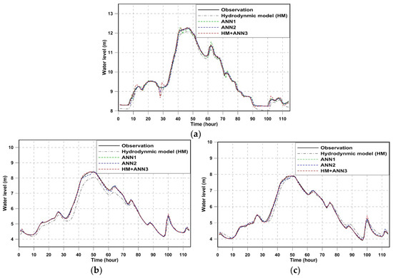
Figure 10.
One-hour lead time water levels calculated by various forecasting models for flood event 2 (15 July 2004–19 July 2004): (a) Paldang Bridge; (b) Banpo Bridge; (c) Hangang Bridge.

Figure 11.
Two-hour lead time water levels calculated by various forecasting models for flood event 2 (15 July 2004–19 July 2004): (a) Paldang Bridge; (b) Banpo Bridge; (c) Hangang Bridge.
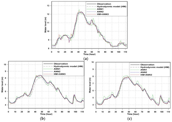
Figure 12.
Three-hour lead time water levels calculated by various forecasting models for flood event 2 (15 July 2004–19 July 2004): (a) Paldang Bridge; (b) Banpo Bridge; (c) Hangang Bridge.
Two statistics, i.e., the Nash–Sutcliffe efficiency coefficient (NSE) and RMSE, were used to evaluate the accuracy of different forecasting models. The values of two statistics for training periods are summarized in Table 6, and the best results for each location according to each performance metric are highlighted in bold. NSE and RMSE indicate that the hydrodynamic model alone has relatively low accuracy compared to other forecasting models. Forecasting the accuracy of ANN1 decreases with the longer lead time of forecasting, which is naturally expected as ANN1 only uses the historical observations to forecast water levels. Forecasts by the hybrid approach are most accurate at the Paldang Bridge, while ANN2 also shows good performance at the Banpo Bridge and Hangang Bridge.
Table 6.
Statistical comparison of model performances for the training periods.
The validation results are shown in Table 7 and the best results are also highlighted in bold. It is immediately obvious from the table that the hybrid approach is the most accurate based on the RMSE and NSE when applied to all three locations, and the accuracy reduces with the increasing lead time of forecasting. ANN2 showed better accuracy in the model training at the Banpo Bridge and Hangang Bridge, while it shows worse performance than the hybrid approach in the model validation. The prediction accuracy of ANN1 decreases as lead time increases, and it performs worse than the hydrodynamic model for 3-h lead time forecasting at the Hangang Bridge. The reduction in the simulation errors of the hydrodynamic model is evident after error correction by ANNs, which implies that coupling a hydrodynamic model and an ANN (as opposed to only using a hydrodynamic model or an ANN) results in highly accurate predictions of water levels. For 1-h lead time forecasting, the hybrid approach achieved 70%, 80%, and 76% reduction in the RMSE at the Paldang Bridge, Banpo Bridge, and Hangang Bridge, respectively, when compared with the hydrodynamic model. In addition, the reduction in the RMSE by applying the hybrid approach are 18%, 13%, and 33% at 3 locations when compared with the ANN2, which indicates the better performance of a hybrid model compared to an ANN model. For the 2-h lead time forecasting, the hybrid model achieved 65%, 69%, and 65% reduction in the RMSE at the Paldang, Banpo and Hangang Bridges, respectively, when compared with the hydrodynamic model, and the reduction is 26%, 16%, and 33% when compared to the ANN2. ANN1 shows less accuracy than the hybrid model and ANN2. The NSE for the hybrid model is over 0.99 when the model is applied for the 1-h or 2-h forecasting at all locations, and it is over 0.98 when it is applied to the 3-h forecasting. The results of this research indicate that the hybrid model performs better than a data-driven model (i.e., ANN1 or ANN2), and a data-driven model has better performances when compared to the physically based model (i.e., hydrodynamic model), which is consistent with the research by Cho and Kim [18].
Table 7.
Statistical comparison of model performances for the validation periods.
5. Conclusions
This study presents the combined application of a physically based hydrodynamic model and a data-driven model for the improvement of flood water level prediction. In order to enhance the performance of the hydrodynamic model, calibration was initially performed by using power functions that describe the relationships between Manning’ s n and discharge for two sub-reaches. The optimized hydrodynamic model performed well when compared to the observed data at gauging stations. Subsequently, the impact of the systematic errors in the optimized hydrodynamic model was significantly reduced by using a complementary data-driven error correction model.
To test the performance accuracy of the hybrid model which combines the hydrodynamic model and ANNs, a comparison of the hydrodynamic model, two water level forecasting models based on ANNs (i.e., ANN1 and ANN2), and the hybrid model (HM+ANN3) was carried out. It was demonstrated that the water level forecasted by the hydrodynamic model is generally less accurate than those by two ANN models (i.e., ANN1 and ANN2). ANN1 is a data-driven forecasting model, which was developed based on the historical observations. Since the model only uses the historical data, the accuracy of the model decreases as the lead time of forecasting increases. As the hydrodynamic forecast model need predicted boundary conditions as inputs, ANN2 also included the predicted boundary conditions as potential inputs. By providing the same types of data for the hybrid model and ANN2, it is reasonable to test if a hybrid model performs better than an ANN. Though the same data were provided for constructing these two models, the outputs of the hydrodynamic model, e.g., computed water levels and their time derivatives, and historical errors between computed and observed water levels were additionally included in the input candidates of the error correction model (ANN3).
A PMI-based input variable selection method was employed to identify suitable inputs to ANN models. The selected variables for predicting water levels or simulating errors can play a crucial role in theoretically describing physical mechanisms. The ANNs developed based on the PMI-based input variable selection provide efficient and accurate predictions by mapping specific relationships between the inputs and output. ANN-based error correction approach for a hydrodynamic model presented in this study is simple to implement and provides the uncertainty reduction in water level forecasting. This method can implicitly account for a range of uncertainties that are contained in the deterministic model output time series derived offline prior to application.
The comparison of the model performances showed that the hybrid model performs better than the individual hydrodynamic model and ANNs in terms of RMSE and NSE. Though ANN2 is more accurate than the hybrid model during the training period at the Banpo Bridge, it does not show better performance for validation data. The predictions produced by the hybrid model can capture the variation pattern of the forecasted water level by describing the rising and falling tendencies of the water levels in a fairly accurate manner. The results of this study indicate that aggregating a physically based hydrodynamic model and a data-driven model rather than only applying a hydrodynamic model or a data-driven model can fully exploit different aspects of the physical system to minimize the prediction errors between estimated and observed water levels. The findings of this study suggest that the combination of a hydrodynamic flow model and an ANN can be applied for water level forecasting with high accuracy. It should be noted that this study focused on error correction in the forecasting mode, given the assumption that the hydrodynamic model is executed in the forecasting mode with the same accuracy as in the simulation mode. The accuracy of water level forecasting can be different depending on the accuracy of the predicted boundary conditions of the hydrodynamic model.
Author Contributions
Conceptualization, L.L. and K.S.J.; methodology, L.L. and K.S.J.; software, L.L. and K.S.J.; investigation, L.L. and K.S.J.; data curation, L.L.; writing—original draft preparation, L.L.; writing—review and editing, L.L.; supervision, K.S.J.; project administration, K.S.J.; funding acquisition, K.S.J. All authors have read and agreed to the published version of the manuscript.
Funding
This work was supported by the Korea Environmental Industry and Technology Institute (KEITI) (Grant number: 2022003460001).
Conflicts of Interest
The authors declare no conflict of interest.
References
- Didovets, I.; Krysanova, V.; Bürger, G.; Snizhko, S.; Balabukh, V.; Bronstert, A. Climate change impact on regional floods in the Carpathian region. J. Hydrol. Reg. Stud. 2019, 22, 100590. [Google Scholar] [CrossRef]
- Qin, P.; Xu, H.; Liu, M.; Xiao, C.; Forrest, K.E.; Samuelsen, S.; Tarroja, B. Assessing concurrent effects of climate change on hydropower supply, electricity demand, and greenhouse gas emissions in the Upper Yangtze River Basin of China. Appl. Energy 2020, 279, 115694. [Google Scholar] [CrossRef]
- Schlogl, M.; Fuchs, S.; Scheidl, C.; Heiser, M. Trends in torrential flooding in the Austrian Alps: A combination of climate change, exposure dynamics, and mitigation measures. Clim. Risk Manag. 2021, 32, 100294. [Google Scholar] [CrossRef]
- Juárez, A.; Alfredsen, K.; Stickler, M.; Adeva-Bustos, A.; Suárez, R.; Seguín-García, S.; Hansen, B. A Conflict between Traditional Flood Measures and Maintaining River Ecosystems? A Case Study Based upon the River Lærdal, Norway. Water 2021, 13, 1884. [Google Scholar] [CrossRef]
- Ricci, S.; Piacentini, A.; Thual, O.; Le Pape Le, E.; Jonville, G. Correction of upstream flow and hydraulic state with data assimilation in the context of flood forecasting. Hydrol. Earth Syst. Sci. 2011, 15, 3555–3575. [Google Scholar] [CrossRef]
- Gupta, H.V.; Wagener, T.; Liu, Y. Reconciling theory with observations: Elements of a diagnostic approach to model evaluation. Hydrol. Process. 2008, 22, 3802–3813. [Google Scholar] [CrossRef]
- Abebe, A.J.; Price, R.K. Managing uncertainty in hydrological models using complementary models. Hydrol. Sci. J. 2003, 48, 679–692. [Google Scholar] [CrossRef]
- Torres-Rua, A.F.; Ticlavilca, A.M.; Walker, W.R.; McKee, M. Machine learning approaches for error correction of hydraulic simulation models for canal flow schemes. J. Irrig. Drain. Eng. 2012, 138, 999–1010. [Google Scholar] [CrossRef]
- Humphrey, G.B.; Gibbs, M.S.; Dandy, G.C.; Maier, H.R. A hybrid approach to monthly streamflow forecasting: Integrating hydrological model outputs into a Bayesian artificial neural network. J. Hydrol. 2016, 540, 623–640. [Google Scholar] [CrossRef]
- Konapala, G.; Kao, S.C.; Painter, S.L.; Lu, D. Machine learning assisted hybrid models can improve streamflow simulation in diverse catchments across the conterminous US. Environ. Res. Lett. 2020, 15, 104022. [Google Scholar] [CrossRef]
- Yang, S.; Yang, D.; Chen, J.; Santisirisomboon, J.; Lu, W.; Zhao, B. A physical process and machine learning combined hydrological model for daily streamflow simulations of large watersheds with limited observation data. J. Hydrol. 2020, 590, 125206. [Google Scholar] [CrossRef]
- Shamseldin, A.Y.; O’Connor, K.M. A non-linear neural network technique for updating of river flow forecasts. Hydrol. Earth Syst. Sci. 2001, 5, 577–598. [Google Scholar] [CrossRef]
- Brath, A.; Montanari, A.; Toth, E. Neural networks and non-parametric methods for improving real-time flood forecasting through conceptual hydrological models. Hydrol. Earth Syst. Sci. 2002, 6, 627–639. [Google Scholar] [CrossRef]
- Yu, P.S.; Chen, S.T. Updating real-time flood forecasting using a fuzzy rule-based model. Hydrol. Sci. J. 2005, 50, 265–278. [Google Scholar] [CrossRef][Green Version]
- Bogner, K.; Kalas, M. Error-correction methods and evaluation of an ensemble based hydrological forecasting system for the Upper Danube catchment. Atmos. Sci. Lett. 2008, 9, 95–102. [Google Scholar] [CrossRef]
- Bogner, K.; Pappenberger, F. Multiscale error analysis, correction, and predictive uncertainty estimation in a flood forecasting system. Water Resour. Res. 2011, 47, W07525. [Google Scholar] [CrossRef]
- Pianosi, F.; Castelletti, A.; Mancusi, L.; Garofalo, E. Improving flow forecasting by error correction modelling in altered catchment conditions. Hydrol. Process. 2014, 28, 2524–2534. [Google Scholar] [CrossRef]
- Cho, K.; Kim, Y. Improving stream prediction in the WRF-Hydro model with LSTM networks. J. Hydrol. 2022, 605, 127297. [Google Scholar] [CrossRef]
- Demissie, Y.K.; Valocchi, A.J.; Minsker, B.S.; Bailey, B.A. Integrating a calibrated groundwater flow model with error-correcting data-driven models to improve predictions. J. Hydrol. 2009, 364, 257–271. [Google Scholar] [CrossRef]
- Xu, T.; Valocchi, A.J.; Choi, J.; Amir, E. Use of machine learning methods to reduce predictive error of groundwater models. Groundwater 2014, 52, 448–460. [Google Scholar] [CrossRef]
- Xu, T.; Valocchi, A.J. Data-driven methods to improve baseflow prediction of a regional groundwater model. Comput. Geosci. 2015, 85, 124–136. [Google Scholar] [CrossRef]
- Azad, A.S.; Sokkalingam, R.; Daud, H.; Adhikary, S.K.; Khurshid, H.; Mazlan, S.N.A.; Rabbani, M.B.A. Water Level Prediction through Hybrid SARIMA and ANN Models Based on Time Series Analysis: Red Hills Reservoir Case Study. Sustainability 2022, 14, 1843. [Google Scholar] [CrossRef]
- Bruen, M.; Yang, J. Combined hydraulic and black-box models for flood forecasting in urban drainage systems. J. Hydrol. Eng. 2006, 11, 589–596. [Google Scholar] [CrossRef]
- Preis, A.; Whittle, A.J.; Ostfeld, A.; Perelman, L. Efficient hydraulic state estimation technique using redued models of urban water networks. J. Water Resour. Plan. Manag. 2011, 137, 343–351. [Google Scholar] [CrossRef]
- Abebe, A.J.; Price, R.K. Information theory and neural networks for managing uncertainty in flood routing. J. Comput. Civ. Eng. 2004, 18, 373–380. [Google Scholar] [CrossRef]
- Srinivasulu, S.; Jain, A. River flow prediction using an integrated approach. J. Hydrol. Eng. 2009, 14, 75–83. [Google Scholar] [CrossRef]
- Maier, H.R.; Jain, A.; Dandy, G.C.; Sudheer, K.P. Methods used for the development of neural networks for the prediction of water resource variables in river systems: Current status and future directions. Environ. Model. Sofw. 2010, 25, 891–909. [Google Scholar] [CrossRef]
- Ayvaz, M.T. A linked simulation-optimization model for simultaneously estimating the Manning’s surface roughness values and their parameter structures in shallow water flows. J. Hydrol. 2013, 500, 183–199. [Google Scholar] [CrossRef]
- Bowden, G.J.; Dandy, G.C.; Maier, H.R. Input determination for neural network models in water resources applications. Part 1–background and methodology. J. Hydrol. 2005, 301, 75–92. [Google Scholar] [CrossRef]
- Li, L.; Jun, K.S. Distributed parameter unsteady flow model for the Han River. J. Hydro-Environ. Res. 2018, 21, 86–95. [Google Scholar] [CrossRef]
- Cunge, J.A.; Holly, F.M.; Verwey, A. Practical Aspects of Computational River Hydraulics; Pitman: Toronto, ON, Canada, 1980. [Google Scholar]
- Liggett, J.A.; Cunge, J.A. Numerical Methods of Solution of the Unsteady Flow Equations. Unsteady Flow in Open Channels; Mohmmod, K., Yevjevich, V., Eds.; Water Resources Publications: Fort Collins, CO, USA, 1975; pp. 89–182. [Google Scholar]
- Holly, F.M.; Yang, J.C.; Schwarz, P.; Schaefer, J.; Hsu, S.H.; Einhellig, R. Numerical Simulation of Unsteady Water and Sediment Movement in Multiply Connected Networks of Mobile-Bed Channels; IIHR Report No. 343; Iowa Institute of Hydraulic Research: Iowa City, IA, USA, 1990. [Google Scholar]
- Ramesh, R.; Dattam, B.; Bhallamudi, S.; Narayana, A. Optimal Estimation of Roughness in Open-Channel Flows. J. Hydraul. Engrg. 2000, 126, 299–303. [Google Scholar] [CrossRef]
- Ding, Y.; Jia, Y.; Wang, S. Identification of Manning’s roughness coefficients in shallow water flows. J. Hydraul. Eng. 2004, 130, 501–510. [Google Scholar] [CrossRef]
- Ding, Y.; Wang, S.S.Y. Identification of Manning’s roughness coefficients in channel network using adjoint analysis. Int. J. Comput. Fluid Dyn. 2005, 19, 3–13. [Google Scholar] [CrossRef]
- Fread, D.L.; Smith, G.F. Calibration technique for 1-D unsteady flow models. J. Hydraul. Div. 1978, 104, 1027–1044. [Google Scholar] [CrossRef]
- Li, L.; Chung, E.-S.; Jun, K.S. Robust parameter set selection for a hydrodynamic model based on multi-site calibration using multi-objective optimization and minimax regret approach. Water Resour. Manag. 2018, 32, 3979–3995. [Google Scholar] [CrossRef]
- Doherty, J. Visual PEST: Model-Independent Parameter Estimation; Watermark Computing & Waterloo Hydrogeologic: Waterloo, ON, Canada, 2000. [Google Scholar]
- Hutton, C.J.; Vamvakeridou-Lyroudia, L.S.; Kapelan, Z.; Savic, D.A. Real-time modelling and data assimilation techniques for improving the accuracy of model. Hydrol. Sci. J. 2010, 48, 679–692. [Google Scholar]
- Maier, H.R.; Dandy, G.C. Neural networks for the prediction and forecasting of water resources variables: A review of modeling issues and applications. Environ. Model. Softw. 2000, 15, 101–124. [Google Scholar] [CrossRef]
- Bodri, L.; Cermak, V. Prediction of extreme precipitation using a neural network: Application to summer flood occurrence in Moravia. Adv. Eng. Softw. 2000, 31, 311–321. [Google Scholar] [CrossRef]
- He, J.; Valeo, C.; Chu, A.; Neumann, N.F. Prediction of event-based stormwater runoff quantity and quality by ANNs developed using PMI-based input selection. J. Hydrol. 2011, 400, 10–23. [Google Scholar] [CrossRef]
- Masters, T. Practical Neural Network and Expert Systems; Kluwer Academic Publishers: Norwell, MA, USA, 1993. [Google Scholar]
- Hsu, K.L.; Gupta, H.V.; Sorroshian, S. Artificial neural network modelling of the rainfall-runoff process. Water Resour. Res. 1995, 31, 2517–2530. [Google Scholar] [CrossRef]
- Thirumalaiah, K.; Deo, M.C. River stage forecasting using artificial neural networks. J. Hydrol. Eng. 1998, 3, 26–32. [Google Scholar] [CrossRef]
- Lange, N.T. New mathematical approaches in hydrological modelling-An application of artificial neural networks. Phys. Chem. Earth 1999, 24, 31–35. [Google Scholar] [CrossRef]
- Luk, K.C.; Ball, J.E.; Sharma, A. A study of optimal model lag and spatial inputs to artificial neural network for rainfall forecasting. J. Hydrol. 2000, 227, 56–65. [Google Scholar] [CrossRef]
- ASCE Task Committee on Application of Artificial Neural Networks in Hydrology. Artificial Neural Networks in Hydrology. I: Preliminary Concepts. J. Hydrol. Eng. 2000, 5, 115–123. [Google Scholar] [CrossRef]
- ASCE Task Committee on Application of Artificial Neural Network in Hydrology. Artificial Neural Networks in Hydrology, II: Hydrologic Application. J. Hydrol. Eng. 2000, 5, 124–136. [Google Scholar] [CrossRef]
- Guyon, I.; Elisseeff, A. An introduction to variable and feature selection. J. Mach. Learn. Res. 2003, 3, 1157–1182. [Google Scholar]
- Chow, T.W.S.; Huang, D. Estimating optimal feature subsets using efficient estimation of high-dimensional mutual information. IEEE Trans. Neural Netw. 2005, 16, 213–224. [Google Scholar] [CrossRef]
- Battiti, R. Using mutual information for selecting features in supervised neural net learning. IEEE Trans. Neural Netw. 1994, 5, 537–550. [Google Scholar] [CrossRef]
- May, R.J.; Maier, H.R.; Dandy, G.C.; Fernando, T.M.K.G. Non-linear variable selection for artificial neural networks using partial mutual information. Environ. Model. Softw. 2008, 23, 1312–1326. [Google Scholar] [CrossRef]
- May, R.J.; Dandy, G.C.; Maier, H.R.; Nixon, J.B. Application of partial mutual information variable selection to ANN forecasting of water quality in water distribution systems. Environ. Model. Softw. 2008, 23, 1289–1299. [Google Scholar] [CrossRef]
- Sharma, A. Seasonal to interannual rainfall probabilistic forecasts for improved water supply management: Part 1—A strategy for system predictor identification. J. Hydrol. 2000, 239, 232–239. [Google Scholar] [CrossRef]
- Yue, Z.; Ai, P.; Xiong, C.; Hong, M.; Song, Y. Mid-to long-term runoff prediction by combining the deep belief network and partial least-squares regression. J. Hydroinformatics 2020, 22, 1283–1305. [Google Scholar] [CrossRef]
- Harrold, T.I.; Sharma, A.; Sheather, S. Selection of a kernel bandwidth for measuring dependence of hydrologic time series using the mutual information criterion. Stoch. Environ. Res. Risk Assess. 2001, 15, 310–324. [Google Scholar] [CrossRef]
- Galelli, S.; Humphrey, G.B.; Maier, H.R.; Castelletti, A. An evaluation framework for input variable selection algorithm for environmental data-driven models. Environ. Model. Softw. 2014, 62, 33–51. [Google Scholar] [CrossRef]
- Akaike, H. A new look at the statistical model identification. IEEE Trans. Autom. Control. 1974, 19, 7716–7723. [Google Scholar] [CrossRef]
- Torres-Rua, A.F. Bayesian Data-Driven Models for Irrigation Water Management. Ph.D. Thesis, Utah State University, Logan, UT, USA, 2011; p. 979. [Google Scholar]
Publisher’s Note: MDPI stays neutral with regard to jurisdictional claims in published maps and institutional affiliations. |
© 2022 by the authors. Licensee MDPI, Basel, Switzerland. This article is an open access article distributed under the terms and conditions of the Creative Commons Attribution (CC BY) license (https://creativecommons.org/licenses/by/4.0/).