Feasibility of Traditional Open Levee System for River Flood Mitigation in Japan

Abstract

An open levee system is a traditional flood mitigation system for reducing the expansion of inland flooding and decreasing the peak flow. However, there have been few quantitative studies on its feasibility. Furthermore, the differences in applicability depending on the topography and the construction of continuous levees have not been fully examined. We studied its feasibility based on simulations in the Kuji River area, where the vast Typhoon Hagibis occurred. Morphological models representing the past (the 1940s) and the present (2019), obtained by modifying the highly accurate digital elevation models (DEM) via the tracing of aerial photos, were applied to a 2D unsteady flow simulation model to reveal the effects of the levee system on river hydrography and overland flood behavior. The results indicated that inundation flow through an open area decreased both inundation duration and depth, while the reduction of peak discharge is relatively insignificant at approximately 10%. The sub levees are not adequate under the current conditions and floodwater volume, and their effectiveness depends on the surrounding conditions, such as the development of continuous levees.

1. Introduction

River flood is one of the most catastrophic disasters, causing many human casualties and economic losses every year worldwide [1,2]. Climate change has resulted in an intensified hydrological cycle [3,4], and the river flood risk has been shown to increase, both globally and regionally [5,6]. Hirabayashi et al. (2013) [7] pointed out that under the RCP8.5 scenario, the frequency of river floods will increase by over 42% for the global land area. In addition, the increase in flood risks due to climate change varies by region, with increases in flood-prone populations and cropland being more pronounced in South and East Asia [8]. Based on these projections, various regions have estimated the risks associated with climate change and considered countermeasures [9,10].

The industrialized world has relied heavily on flood control to mitigate flood hazards; however, this has been criticized for harming riverine ecosystems and increasing the long-term flood risk [11,12]. Alternative management concepts have emerged, emphasizing the integration between land and water management and structural and nonstructural measures [13]. In recent years, the concept of ecosystem-based disaster risk reduction (Eco-DRR) has been proposed, and it is hoped that disaster prevention measures will enhance ecosystem functions [14]. Examples of such measures include the conservation of wetlands and flood plains [15,16], the utilization of the storage function of rice paddies [17,18], and disaster risk reduction through land use guidance [19,20] and multiple inundation controls by natural landforms and artificial levees [21,22,23].

In Japan, 70% of the country’s land area is mountainous, while the floodplain area is relatively small. In addition, rivers in Japan have steeper slopes and experience higher rainfall than those in Europe and the US, resulting in high flood flows and flood damage [24]. Various regional flood control techniques and traditional knowledge have been developed to secure cultivated land on narrow floodplains [25]. One example is the open levee system (called “Kasumi-Tei” in Japanese) which has two functions [26]: one is to block overland floodwater and drain it into the river, the other is to reduce the peak flow rate downstream by acting as a dry reservoir. The growing threat of large-scale floods is currently driving the social implementation of the system. Since the system is designed to avoid fatal damage in exchange for the risk of flooding, it is essential to present the risks and benefits of the system (which may vary with location and arrangement) for consensus building. The robustness of an open levee system against a large-scale flood is also not well understood. Therefore, a comprehensive understanding of this system requires a quantitative assessment by applying a computational model to evaluate the interaction between the open levee system and the river–floodplain system. Previous studies on this system include flood mitigation evaluation using geomorphological considerations [26] and two-dimensional (2D) flood calculation [27]. These studies have enabled us to understand the significance of the levee arrangements and their effects on flood control. Some case studies addressing its Eco-DRR functions have shown the balance between flood control, environmental and agricultural benefits, and risks of allowing floodwaters to flow from open levees [28,29]. All of these demonstrate the advantages of this open levee system over flood control by continuous levees. However, few studies simultaneously address the risks and benefits of this system. Globally, nature-oriented flood-protection measures such as “Room for the River” are expanding river corridors [30]. However, there is no discussion about a system that allows inundation in residential and production areas such as Japan’s open levee system.

This study aims to evaluate the flood control effectiveness of the traditional open levee systems on alluvial fan and discuss issues regarding their future operation and management. Specifically, a 2D flood-simulation model was applied to a real flood during Typhoon Hagibis in 2019 in the Kuji River which has open levees. The model was then applied in conditions which represent changes in levees, such as levee construction, open levee closure, and sub levee installing, to evaluate their impact on flood behavior. Finally, we discuss how to implement traditional flood control systems for risk reduction in floodplains during unprecedented floods exceeding planning levels.

2. Materials and Methods

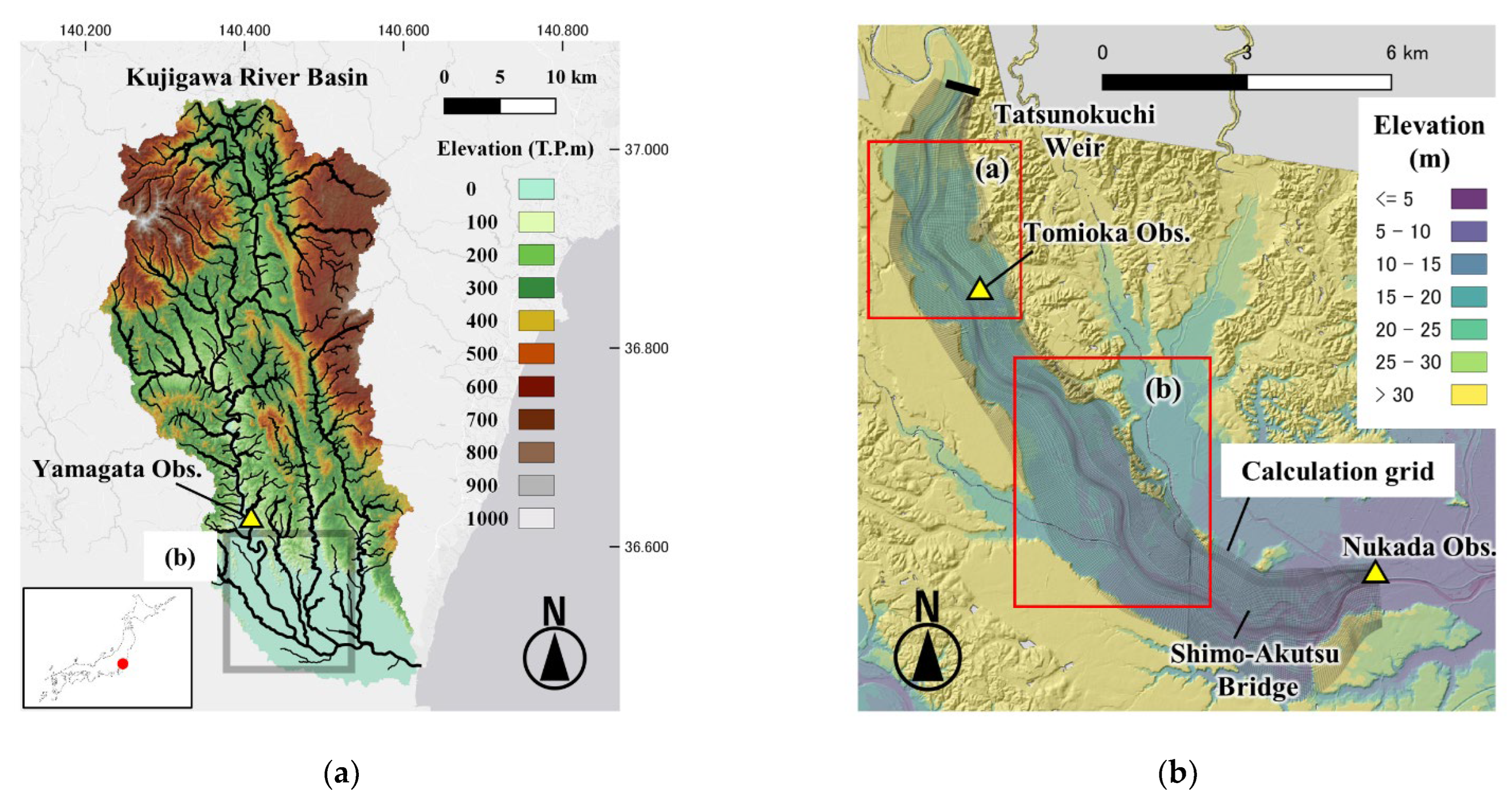
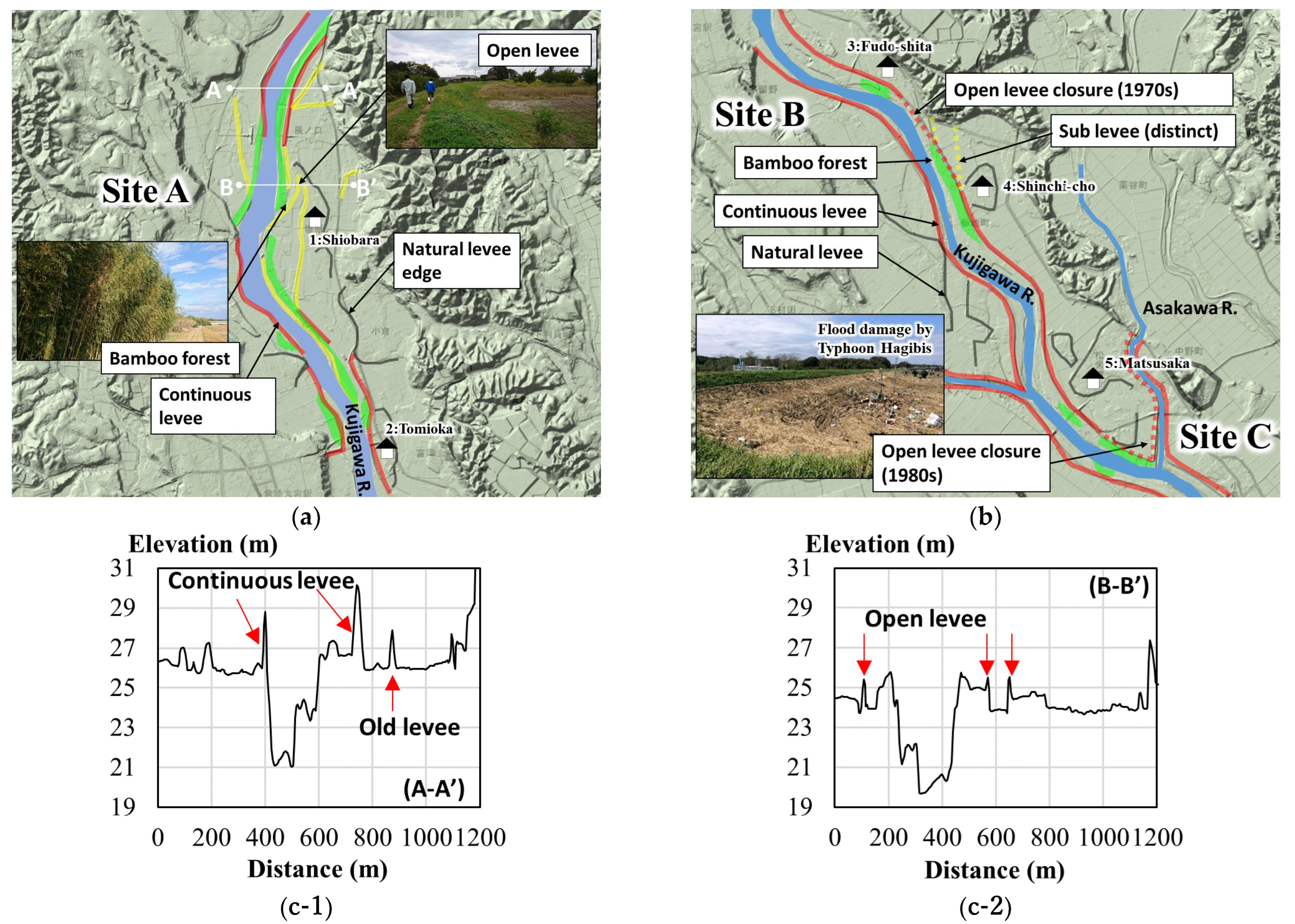
2.1. Study Site

The study site, the Kuji River, flows through Ibaraki Prefecture, east of Japan, about 120 km east of Tokyo (Figure 1). Its basin area is 1490 km² and is mainly covered with forest (55.8%). The average annual rainfall there is approximately 1300 mm. The Kuji River flows mainly through a mountainous area. From the Tatsunokuchi area, it runs into the alluvial lowland. The longitudinal slope in this section is about 1/800 to 1/2000. Overall, the floodplain is consisted of residential area (12%), paddy field (56%), cropland (17%), and forest (12%).

The Kuji River is known for its well-preserved open levees and flood prevention forests (Figure 2) [31]. The existing open levees in the Kuji River are small in scale, about 1 or 2 m above ground level and about 3 m wide (Figure 2a,c-2). They extend upstream and connect to the naturally formed microtopography (natural levees). Flood control forests, mainly bamboo, made to prevent intrusion of sediment and debris intrusion, are distributed across the inner areas of the levees. The old settlements in the floodplain are located on natural levees which are relatively safe from flooding, and they are protected on multiple layers by flood control forests, open levees, and natural levees. When large-scale floods occur, the flood flows back through the open part of levees and inundates even residential areas in case. However, the system leads to water inundating allowed areas and drain through the open part for minimizing the damages. These traditional flood control systems were once found further downstream as well. However, with the construction of continuous levees starting around 1910, the system gradually disappeared. For example, levees at downstream of floodplain (Site B) or upstream side of tributary confluence (site C) had remained unbuilt for keep drain function until 70–80 s, as shown red dash lines in Figure 2b. Since the continuous levee construction brought the progress of safety, it led to agricultural development on the floodplain. As a result, the microelevation (or old levee) that could work as sub levees behind the continuous levee were altered. The sub levee in Site B in Figure 2b indicated by the yellow dash line was found in aerial photos taken in the 1960s, but it disappeared by 1975 due to development. In addition, in recent years, the development area has expanded to include areas with a high geomorphological risk of flooding, such as back marshes and former river channels [32].

Typhoon Hagibis caused severe flood in the Kuji River on 12 October 2019. The average rainfall in the basin over two days was 255 mm, exceeding the postwar maximum of 214 mm in1986. The recurrence probability of the rainfall was estimated at 180 years, which exceeded the levels for formulated basic river maintenance policy (150 years) in this river [33], and the peak flow rate at Yamagata Observatory was estimated at 3700 m³/s (except reduction due to upstream flooding) against the planning flow rate of 4000 m³/s. The peak water level was 5.7 m at Tomioka Observatory, which has a caution level of 3.5 m [33]. This unprecedented flood resulted in three bank breaches and three bank damages, and inundated 914 houses and 1180 ha of land, especially on the left bank of the Kuji River. The inundation depth was extremely damaging to the rivers in east Japan, such as the Chikuma (Shinano) River and the Abukuma River [34].

2.2. Two-Dimensional River Flood Simulation

2.2.1. Outline

A 2D flood flow simulation was conducted to evaluate the effect of continuous and open levees on the inundation behavior in the Kuji River. To represent flow interaction between the river channel and floodplain, both areas were modeled as one computational domain. Model validation was carried out using the flood data of Typhoon Hagibis in 2019. A series of model simulations was carried out by varying the location of levees (continuous levees, open levees, and sub levees) as described in Section 2.2.3. The calibrated model was also applied to floods of different levels; the peak discharges were 1600 m³/s (equivalent to the real flood occurred in 13 July 1999) and 2500 m³/s.

2.2.2. Model Description

The simulation was performed using Nays2DH solver on iRIC Software (https://i-ric.org/). It can conduct 2D depth-averaged flow simulation. It includes the general curvilinear coordinate system grid generator to allow for the direct consideration of boundary, and orthogonal coordinate system data are converted to the coordinate system in the software.

The model has been applied in many flow field situations [35], for instance, a numerical experiment in open channel flow [36] and river flow with vegetation resistance [37]. The basic equations in an orthogonal coordinate system ($x$,$y$) are shown in Equations (1)–(3) [38]:

(Continuity equation)

$$\frac{\partial h}{\partial t}+\frac{\partial \left(hu\right)}{\partial x}+\frac{\partial \left(hv\right)}{\partial y}=0$$

(1)

(Momentum equations in $x$- and $y$-directions)

$$\frac{\partial \left(uh\right)}{\partial t}+\frac{\partial \left(h{u}^2\right)}{\partial x}+\frac{\partial \left(huv\right)}{\partial y}=-gh\frac{\partial H}{\partial x}-\frac{g{n}_m{}^{2}u\sqrt{u^2+v^2}}{\sqrt[3]{h}}+D^x+\frac{F_x}{\rho }$$

(2)

$$\frac{\partial \left(vh\right)}{\partial t}+\frac{\partial \left(huv\right)}{\partial x}+\frac{\partial \left(hu{v}^2\right)}{\partial y}=-gh\frac{\partial H}{\partial y}-\frac{g{n}_m{}^{2}v\sqrt{u^2+v^2}}{\sqrt[3]{h}}+D^y+\frac{F_y}{\rho }$$

(3)

where $h$ is the water depth; $t$ is the time; $u$ and $v$ are the depth-averaged velocity in the $x$- and $y$-directions, respectively; $g$ is the gravitational acceleration; and $H$ is the total water depth. In the model, the bottom friction was set using Manning’s roughness parameter $n_m$.

The diffusion terms in the $x$- and $y$-directions are expressed as (4) and (5), respectively. Here, ${\nu }_t$ is the eddy viscosity coefficient given by a turbulence model called the zero-equation model, expressed as (6).

$$D^x=\frac{\partial }{\partial x}\left[{\nu }_{t}h\frac{\partial u}{\partial x}\right]+\frac{\partial }{\partial y}\left[{\nu }_{t}h\frac{\partial u}{\partial y}\right]$$

(4)

$$D^y=\frac{\partial }{\partial x}\left[{\nu }_{t}h\frac{\partial v}{\partial x}\right]+\frac{\partial }{\partial y}\left[{\nu }_{t}h\frac{\partial v}{\partial y}\right]$$

(5)

$${\nu }_t=\frac{\kappa }{6}{u}_{*}h$$

(6)

where $\kappa$: Kàrmàn coefficient (=0.4), $u_{*}$: bottom friction velocity (m/s).

External force terms such as vegetation resistance are considered as drag force with drag coefficients $C_d$ as Equations (7) and (8). Here, $a_s$ is the area of interception by vegetation per unit volume, and $h_v$ is height at which vegetation resistance acts (i.e., smaller of the water depth and vegetation height).

$$\frac{F_x}{\rho }=\frac{1}{2}{C}_d{a}_s{h}_{v}u\sqrt{u^2+v^2}$$

(7)

$$\frac{F_y}{\rho }=\frac{1}{2}{C}_d{a}_s{h}_{v}v\sqrt{u^2+v^2}$$

(8)

2.2.3. Topographic Data

Topographic data for the hydraulic simulation representing distributions of the levees at each time stage were prepared using the following procedure. The whole dataset is represented in

Table 1. Topographic conditions for seven simulations.

Case	Topographic Condition
Case-“2019”	Laser-based 5 m resolution DEM (GSI, 2016) overlayed 200 m interval cross-sectional survey data (MLIT, 2013)
Case-“1975”	“2019” data eliminated in area where levees unbuilt in 1975
Case-“1960”	“2019” data eliminated in area where levees unbuilt in 1960
Case-“1948”	“2019” data eliminated in area where levees unbuilt in 1948
Case-“2019R”	“2019” data extracted in river corridor
Case-“1960+”	“1960” data with sub levee
Case-“2019+”	“2019” data with sub levee

.

First, we built a baseline dataset with overlaying the latest cross-sectional data in the channel in 2013 on 5 m-mesh DEM (Digital Elevation Model) data in 2016. The DEM data are available on the website of the Geospatial Information Authority of Japan (GSI) [39] and the channel data is given by MLIT. The channel data are spatially interpolated along the longitudinal direction of calculation grids using function with iRIC software 3.0. Here, we considered this dataset as current condition and named it case-“2019”. Next, a virtual past-terrain model was built by eliminating topographic data on unbuilt continuous levees in each period. Specifically, we traced the area of levees using GIS software with aerial photographs in 2019, 1975, 1960, and 1948 on the GSI website [40]. Then, data elimination and spatial interpolation for case-“2019” were conducted on area where levees were unbuilt before 2019 in each period. These data were called cases-“1975”, “1960”, and “1948”. Although these data represent only presence or absence of continuous levees, and not channel bed evolution or floodplain changes, we ignored these small differences because we did not intend to provide details of reproduction. Data in the 1980s to the 2000s were not dealt with because they have very small differences in continuous levees exist in “2019”. Furthermore, “2019R” was used to represent a complete continuous levee that was prepared by extracting only in the river channel from “2019”.

A dataset for the effect of sub levees, shown in Figure 2b, was also prepared. As with the continuous levee consideration, we added the elevation data to the data in each period. Unfortunately, we could not obtain the actual height of the sub levee, so we assumed it to be the same height as the conjunction on an existing road based on comparing aerial photos. The dataset with sub levee elevation is marked “+”.

In the iRIC software, the elevation in each grid is given as the average of the elevation on the grid corners. Considering the thin structure of levees, the highest values in the grid were applied to grids including a levee.

2.2.4. Common Setting

The computational domain was downstream of the Tatsunokuchi Weir at about 31 km from the mouth to Nukada Observatory at 11.5 km from the mouth, including the main inundation area caused by Typhoon Hagibis in 2019 (Figure 1). The generated calculation grid was about 10 m × 5 m in the channel and 30 m × 10 m in the floodplain. The total number of meshes is 35,574. The calculations were carried out from 20:00 on 12 October 2019 through 17:00 on 13 October 2019 (JST).

In terms of boundary conditions, observation data of the flood of the Typhoon Hagibis were used. The upstream boundary flow rate was set to the same as the observed discharge hydrograph at Yamagata Observatory shown in Figure 3. This hydrograph includes time shift for distance to the upper boundary. The downstream boundary condition is the water level observed at Nukada Observatory in the target flood.

Bed roughness and resistance by vegetation are considered separately. The flow resistance of vegetation, mainly tall bamboo, was incorporated by considering a drag force which is a function of drag coefficient ($C_d$), the area of interception by vegetation per unit volume ($a_s$), and vegetation height ($h_v$) obtained by investigation as 1.2, 0.08 (m⁻¹), and 10 (m), based on a previous study [41]. Manning’s roughness coefficients in the channel and floodplain were calibrated by fitting (1) the simulated water level at Tomioka Observatory (Figure 3) to the observed water level, and (2) the simulated inundation depth to the observed inundation data obtained by GSI [42] as displayed in Figure 4. The depth map data were partially corrected by in-situ flood mark data. Finally, considering the range of the value in previous study [43], the Manning’s coefficients were calibrated as 0.02, 0.03, and 0.06 (m^−1/3s) for low-flow channel, high-flow channel, and floodplain, respectively.

2.2.5. Data Analysis

Snapshots of inundation depth at each step (flooding, peak flow, maximum inundation, and decreasing period) were extracted to find a difference of flood propagation in each topographic condition. The water depth at five residential sites (1: Shiobara and 2: Tomioka, 3: Fudoshita, 4: Shinchi-Cho, and 5: Matsusaka districts shown in Figure 2a,b were extracted to describe the detail of temporal changes in inundation depth. These sites are on the micro-elevation of natural levees in the floodplain. For identification of the effect of sub levee, the result of cases-“1960+”, “1960”, and “2019+” were compared. Case-“1960” was chosen because the sub levee could not be found in 1975. Case-“2019+” was thought to represent how the sub levees work when they are installed in the current conditions. For an objective comparison of damage, the maximum inundation depths for each mesh were organized by thresholds (0.1, 0.45, and 2.0 m) in all the conducted cases. These correspond to an inundation below floor level and above floor level, and the partial destruction of houses (damage rate of 50% or more) [44]. The potential damage costs for residential, paddy, and cropland areas were estimated by a simplified method proposed by Kazama et al. (2009) [45] based on the official manual [44]. For simplicity, only house damage was treated for residential area damage, and the building occupancy rate was assumed to be 10%.

To estimate the effect of open levee on peak flow reduction on the downstream reach, discharge at the Shimo-Akutsu Bridge (Figure 1) was calculated for each condition, including “2019R”. Assuming that the effects of flood wave diffusion and channel storage in the river channel are reflected in the results of case-“2019R”, the differences of each case from “2019R” were thought to result in a peak flow reduction by the open levee.

3. Results

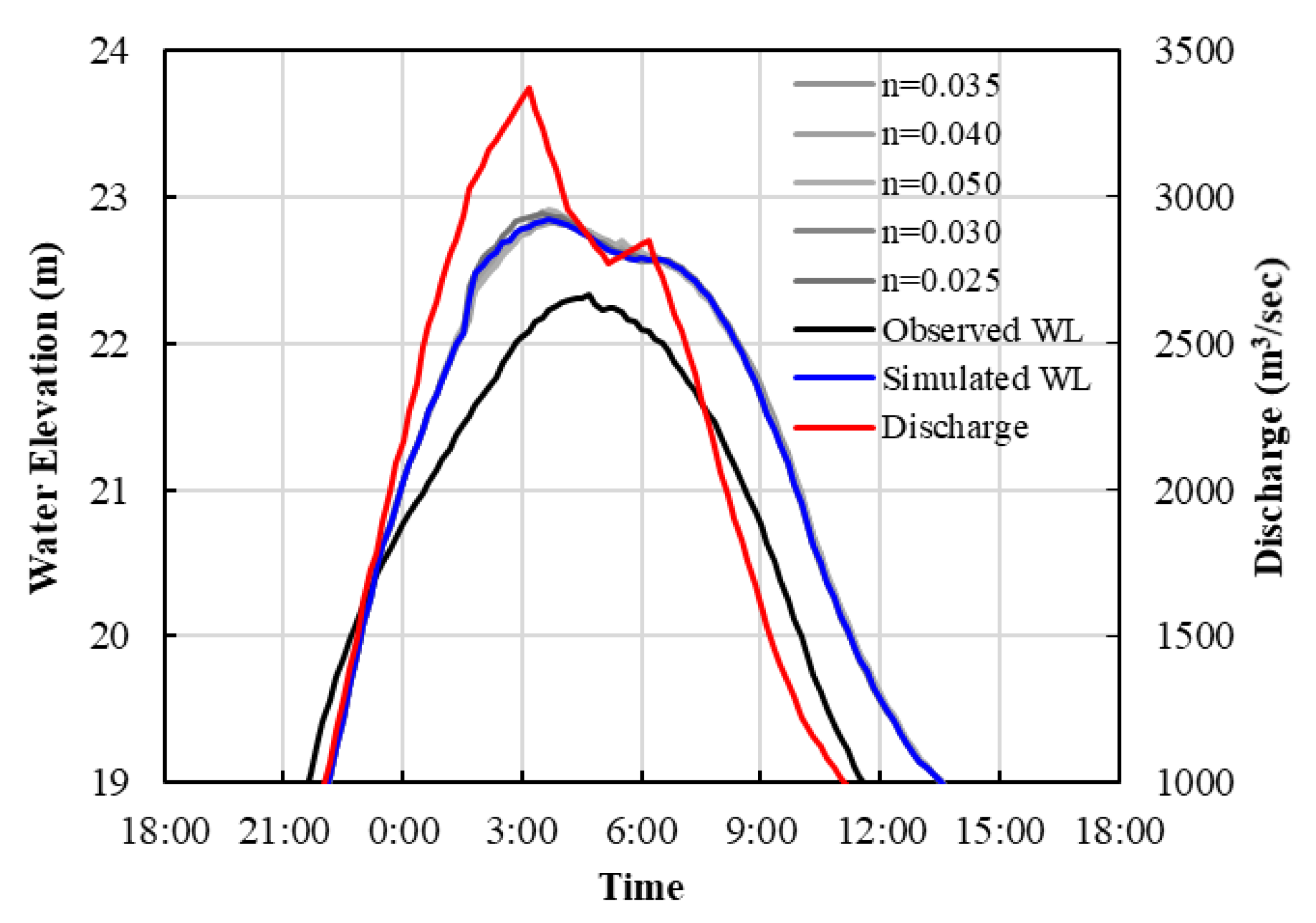
3.1. Model Validation

Figure 3 shows a flow and water level hydrograph at Tomioka Observatory for model calibration. It indicates that the observed water level (black) was close to the estimation (blue). The riverbed roughness is a calibration parameter for this model. However, the channel water level was not sensitive to the roughness coefficient because overland flow into the floodplain increases with greater roughness and increased channel water level reduced the bottom friction. It is possible that the actual hydrograph deforms due to flood wave diffusion because of the distance from the upstream boundary to Yamagata Observatory, which could lead to the overestimation of the input hydrograph. In this study, the reproduction of the inundation area is more important than the reproduction of the channel water level, and the channel roughness parameter was set to a roughness coefficient in a range based on previous study [43].

Figure 4 shows the spatial distribution of the water depths in (a) cases-“1948”, (b) “1975”, and (c) “2019” at the following stages: (1) flooding, (2) peak flow, (3) maximum inundation, and (4) decreasing depicted in Figure 4d. It also includes the actual range of flood in Typhoon Hagibis in 2019 in Figure 4e, which is close to the simulation result of case-“2019” at the period of (3).

Table 2. Root mean square error of depth and correctness of dry/wet for each simulation.

Manning’s n	Low-flow channel	0.02	0.02	0.02	0.03	0.035	0.04	0.05
(m−1/3s)	High-flow channel	0.03	0.04	0.05	0.03	0.035	0.04	0.05
RMS of error of depth (m) $(=\sqrt{\raisebox{1ex}{${{\displaystyle \sum }}_i{\left(h_{cal,i}-h_{obs,i}\right)}^2$}\!\left/ \!\raisebox{-1ex}{$N$}\right.}$, where $h_{cal,i}$: calculated depth, $h_{obs,i}$: observed depth, $i$: suffix of meshes, $N$: nunber of tested meshes. )		0.836	0.923	0.990	0.840	0.896	0.896	0.922
Correctness of dry/wet (%) $(=\left(TP+TN\right)/AREA$, where $TP$: Area that correctly indicates inundation, $TN$: Area that correctly indicates no inundation, and $AREA$: Area of tested floodplain.)		93.3	91.0	85.8	92.9	86.0	86.0	83.4

indicates the root mean square error of inundation depth and correctness of dry/wet for each simulation with different Manning’s n. The correctness of dry/wet are defined as ratio of area that is dry or wet for both observation and simulation to the whole floodplain area. The results indicate that the selected roughness dataset is reasonable. The error values are a little large because we did not consider the actual breaching of old levee on the downstream of district 3, however, we regard this model reasonable enough for comparing the effects of different topography conditions on flood behavior.

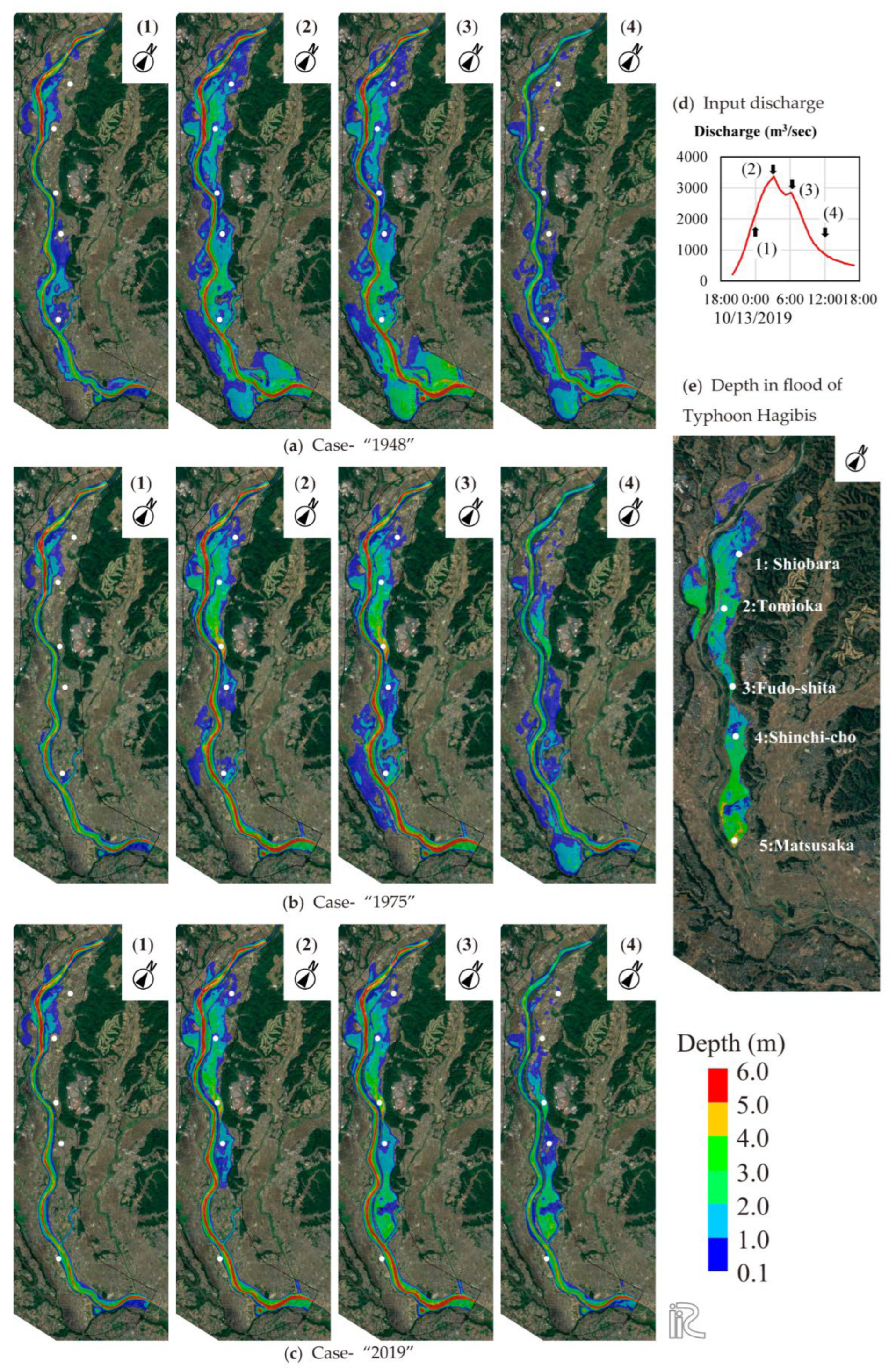
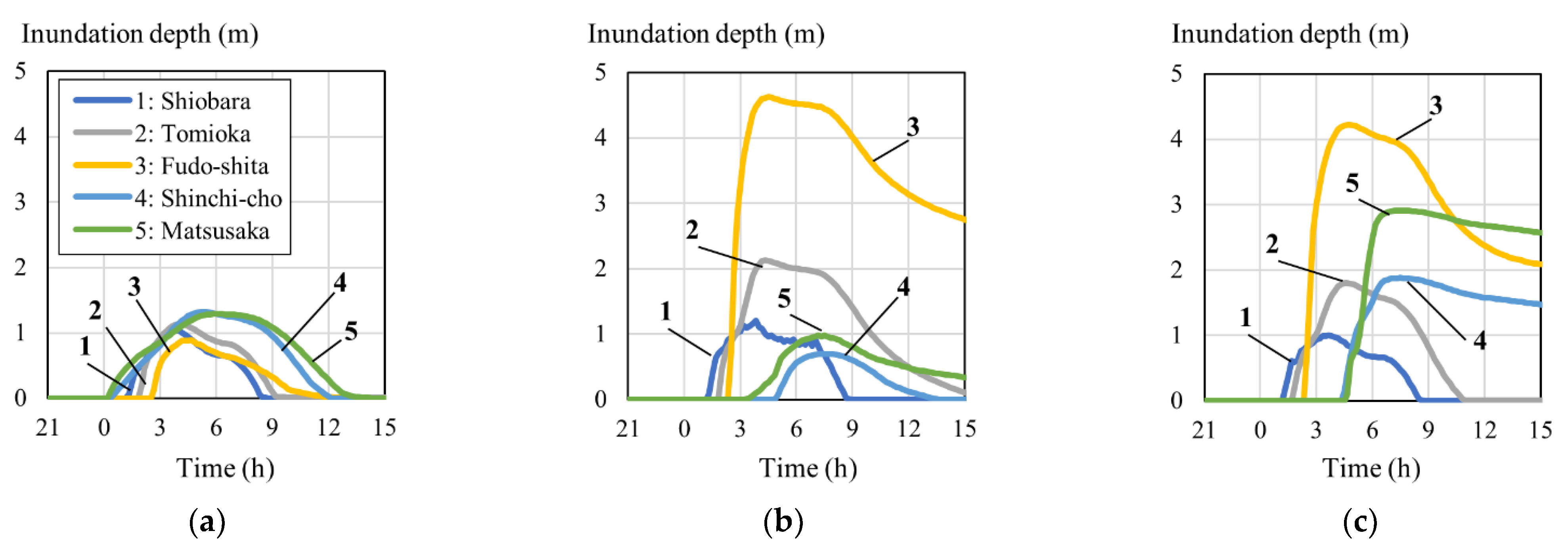
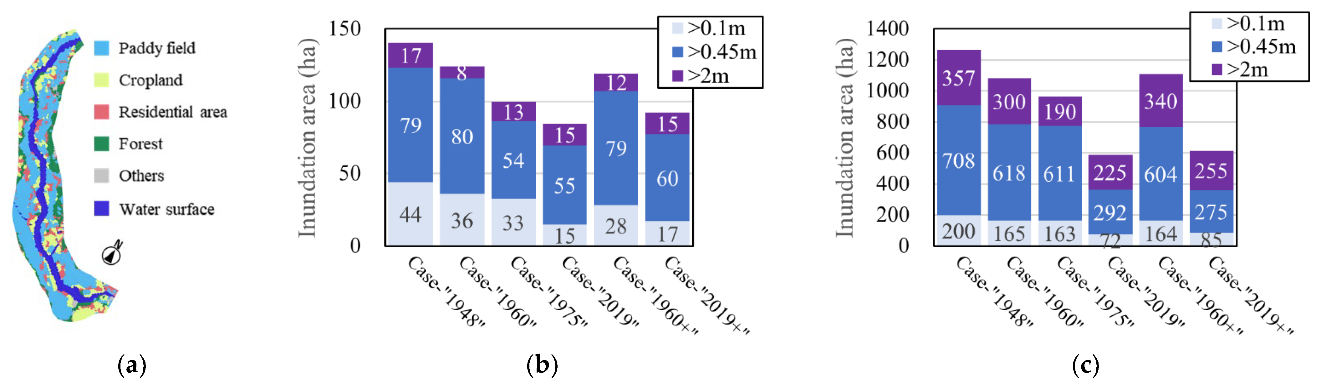
3.2. Flood Behavior on Floodplain

As shown in Figure 4, flood behavior differs in each condition of the levee’s location. As the river water level rises, inundation starts from the opening of the open levees on the left bank (“1” and “2”). The inundation depth increases near the “3” district, where the new levee and the hillside are close together. In this area, the old levee connected to the hillside was still in place, which temporarily blocked the floodwaters from flowing down. After overflowing the old levee and flowing downstream to the “5” district, the floodwaters were blocked again by the levee of the Asakawa River, resulting in a flood depth of over 3 m. A comparison between the topographic conditions was made for each flood stage. In the beginning of flooding (1), inundation was found around the open levee (“1” and “2” districts) in all cases, but only in the 1948 topographic condition did inundation start where the levee had been left unbuilt further downstream in the “4” and “5” districts. At the peak flow period (2), the flood overflowed and inundated broadly in case-“1948”. On the other hand, in condition “1975” and “2019”, the continuous levee significantly controlled the expansion of inundation. Although the open levee in “5” remains in case-“1975”, the inundation to the inner bank was limited. At the time of maximum inundation (3), inundation increased in all cases. However, in decreasing stage (4), the floodwater drained from the open levee in cases-“1948” and “1975”. In contrast, there is still inundation in case-“2019” because of the open levee closure in “5” district.

The results indicate that levee construction may cause spatial differences in the extent of flooding during extensive inundations. Figure 5 shows the time series of water depths for five locations (1,2,3,4,5 in Figure 4) for three topographic conditions. The results for case-“1948” show that there was no significant difference in the inundation depth and dynamics among the sites. In contrast, cases-“1975” and “2019” show apparent differences among the sites. In particular, sites “3”, “4”, and “5”, due to backwatering by levees, showed high inundation depths, whose increasing rates were very high, ranging from about 2 to 3.5 m/hr. In terms of the inundation starting time, in case-“1948”, inundation was concentrated around 0:00–3:00. However, for cases-“1975” and “2019”, inundation occurred later because of levee construction. In districts “4” and “5”, the start of inundation was delayed by 2 to 3 h in the 1975 condition where an open levee remained.

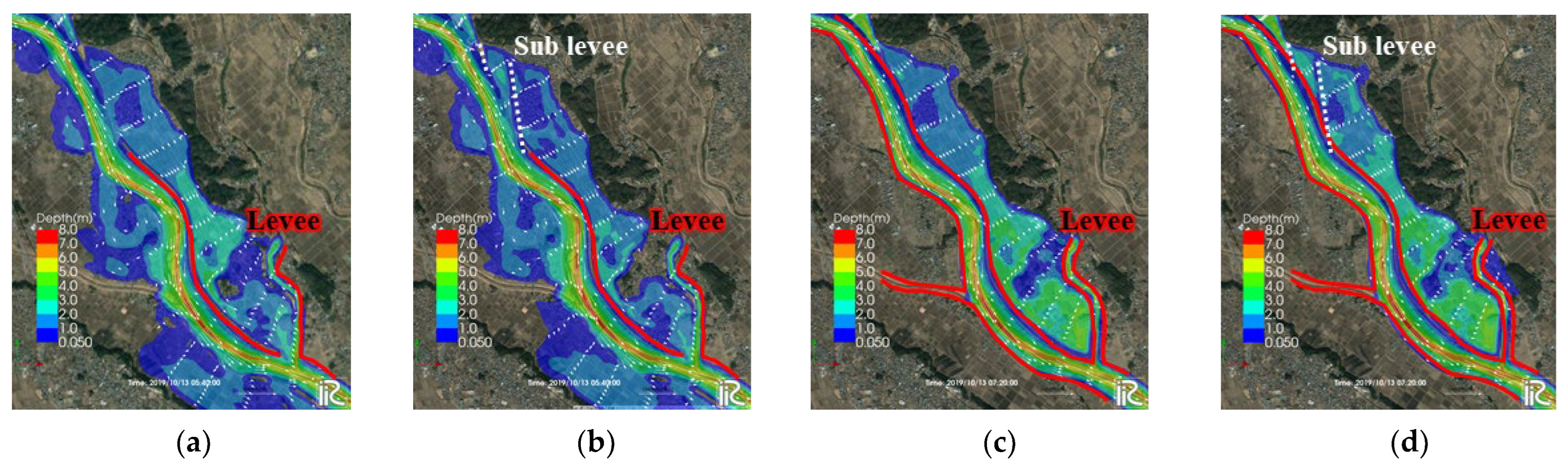
3.3. Effect of Sub Levees

Figure 6 shows the maps of maximum inundation depth in cases with/without sub levee at Site B (Figure 2). In 1960, the continuous levee had not been built completely, and it connected to the sub levee in the floodplain. In the case without the sub levee (case-“1960”), the flood flowed through a section without levees into the floodplain. In contrast, inundation was smaller in the case with a sub levee (case-“1960+”) because it resisted flowing floods. Compared to the cases of 2019, the direct flood flow was shut out completely by the continuous levee. However, it did not work toward the inland flood from upstream. In case-“2019+”, the sub levee blocked the flow temporarily but could not redirect it to the river channel. As a result, they were similarly inundated due to the levee closure on site C. These results show that the effect of the sub levee can be different according to the levee condition.

The construction of levees significantly reduced inundation depth and extent. Figure 7 shows the maximum inundation depths calculated for each computational mesh in each case. The graphs are categorized by depth level and land use (Figure 7a). The figure shows that fewer inundation areas are found in newer topographic conditions. It means that the construction of levees contributes to reducing inundation areas during significant floods. On the other hand, the reduction ratio of inundation depth by the levees differs depending on land use. As shown in Figure 7b, while the area inundated under the floor in residential areas decreased, the percentage flooded above the floor (inundation depth > 0.45 m) increased slightly. The inundation in paddy fields and cropland areas decreased significantly in case-“2019” compared to case-“1975” (Figure 7c).

Figure 8 shows the relations between peak discharge and potential damage cost considering land use and the damage rate for inundation depth. Here, (a), (b), and (c) display values for the total, residential, paddy fields plus cropland area, respectively. Note that the same land use and prices per unit area are applied in all cases of this analysis. The results basically indicate that the higher the flow rate and the older the topographic condition (the fewer levees), the higher the damage cost. However, in detail, that in case”2019” for Typhoon Hagibis (Q_max = 3300) is slightly higher than that in case”1975”. Mainly, the difference in damage in residential areas brought differences in the damage value. In terms of paddy fields and croplands, the values for Typhoon Hagibis are smaller in case”2019” than in case”1975”, but case”1975” is larger for Q_max = 2500.

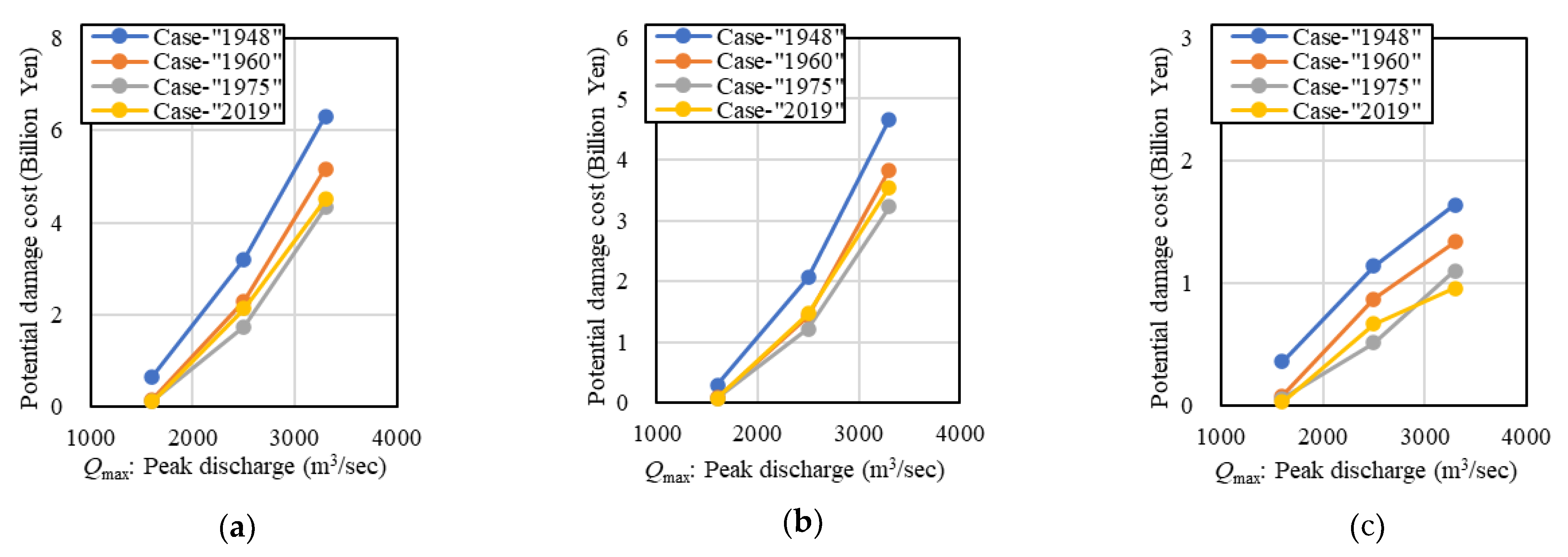
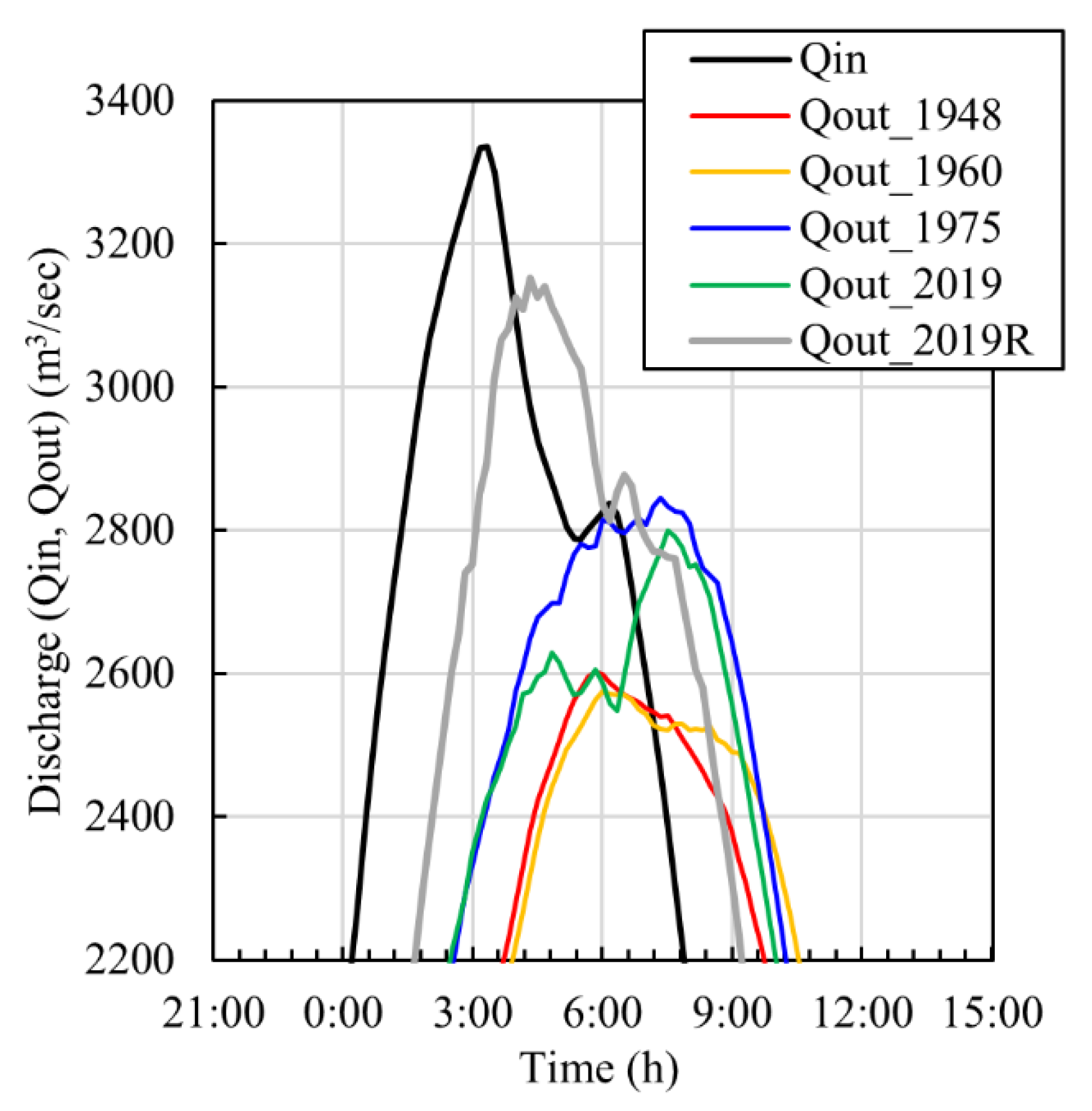
3.4. Peak Flow Reduction

Figure 9 shows the calculated discharge at the Shimo-Akutsu Bridge (Figure 1b) in each case including case-“2019R”. The figure also shows the input flow rate at the upstream end. The peak flow reduction in the target reach is calculated as a difference of peaks between input (upstream) and output (downstream). This result shows that the more the continuous levee is developed, the smaller the peak flow reduction. By contrast, when extending the continuous levee, the peak flow reduction in case-“2019” was more significant than that in case-“1975”. The hydrograph of case-“2019” was skewed near the peak. This is because the floodwaters from the river channel to the floodplain were trapped by the levee and did not return to the river channel, as shown in Figure 4.

4. Discussion

4.1. Effect of Open Levee Systems

In this study, we attempted to assess the effects of the open and continuous levees on flood control by conducting two-dimensional flood simulations based on a topographical model considering the location of the levee. The model was calibrated by the flood data for Typhoon Hagibis in 2019 (Figure 3 and Figure 4, Table 2). The simulation results clearly show that, the higher the number of continuous levees constructed, the less inundation area (Figure 4 and Figure 7), which is a significant flood control effect offered by continuous levees. On the other hand, the levee also caused severe situations. In a case without levees, such as case-“1948”, inundation depths were similar in various parts of the floodplain. However, they were deeper and increased rapidly behind the closure site in the case of completed levees such as case-“2019”, which caused spatial differences in inundation conditions to increase (Figure 5). Tabulation at the inundation depth level also showed no decrease in the area of severely inundated (>2 m) areas (Figure 7). In other words, the presence of levees is likely to increase the degree of damage or cause a spatial imbalance of risk when overflow occurs beyond the protection level of the facilities, especially in residential areas. Although the inundation area was smaller, potential damage values in case-“2019” were estimated to be higher than that in case-“1975” (Figure 8), which quantitatively shows that continuous levee construction could not always reduce damage for floods at levels that cause overflowing. The sub levees could not work in the current condition in the target flood (Figure 6).

It is also hoped that open levees can reduce peak flow similar to a retarding basin. In this simulation, the peak flow reduction in case-“2019” was calculated for up to 10% of input flow in the current condition (Figure 9). However, it was obtained at the expense of severe inundation of the inner levee area. If the open levee at site A was closed, the peak flow reduction would be significantly smaller (Figure 4). Cases where the open levee is in site C, for example, cases-“1960” and “1975”, show that backwater through the open levee is limited. It also implies that the calculated peak flow reduction is overestimated. Conversely, the inundation risk of retaining drain function is low.

Based on the results, the implementation of open levees is discussed. Open levees work as flood drainers or peak flow reducers [28] which are strongly related to the structure and location. In this study, we regard it as a drainer in sites B and C, and a peak flow reducer in site A. The open levee closing in sites B and C had a significant impact on the severe damage. However, the risk for leaving the opening was estimated to be relatively low in the disaster situation. On the other hand, if the open levee at site A was closed, the flooding would not occur, but we would lose a peak flow reducer on the downstream flow. One of the options is modifying the open levee height to rebalance. In such cases, it is useful to conduct multi-level floods risk assessment. In general, open levees have been built historically by residents based on the local balance between inundation risk and benefit of recovery. Before the continuous levees were built, such local defenses would not affect another local site. However, continuous levees altered the spatial risk balance. Therefore, to implement the system in the current levee situation, it is necessary to consider a broader area using appropriate flood simulation.

4.2. Implementation and Management of Open Levees

Typhoon Hagibis reminded us again of the limitations of existing structural measures against unprecedented floods. In response, the MLIT announced a new policy on basin-wide flood control, “River Basin Disaster Resilience and Sustainability by All,” in July 2020 [46]. This policy includes measures other than river channel improvements, e.g., preserving traditional systems such as an open levee and land use regulation.

Based on the findings of this study, the potential implementation of traditional flood control measurement can be discussed. One important point is to view the open levee as part of a comprehensive system that includes topography and other facilities, instead of treating it as a single independent facility. Our simulations showed that whether the past system still works in the current environment is dependent on situation and location. The effectiveness of open levees depends on the exchange of flood flows between the river channel and the floodplain and the resulting flood behavior in the inundation zone. It is essential to evaluate the system or structures in a spatio-temporal framework integrating river corridor and floodplain.

Effort is needed to improve the integrated simulation of flow in the rivers and flood plains. The unstructured grid models have the advantage of offering extreme flexibility in grid generation [47]. One-dimensional and two-dimensional integrated models define linking elements in the one-dimensional node and two-dimensional grid and implement volume interchange between the models [48]. This study applied a 2D model with a general coordinate system structural grid to a river channel and floodplain area as one domain. This method has the advantage of easy grid generation, with no need for connection defining and the utilization of a detailed elevation map without modification. There are two options to improve the model reproducibility. One is to adopt a higher grid resolution, and the other is to adopt a less sensitive model to parameter fitting. Currently, we can obtain sub-meter fine-grid topography by airborne laser-based survey technology, which allows us to extract thin topography, such as that of sub levees. An ALB (Airborne LiDAR Bathymetry) can measure even under the water body, and MLIT has started to use it as a standard method for the periodic river survey [49]. To effectively use these high-resolution DEMs, a technique that extracts features below the grid scale is important for computational load reduction [50]. Recently, progress in computational capabilities and schemes allows large-scale calculations using million-order cells [51], and it is becoming possible to use high-resolution DEM almost as is. In terms of parameter fitting, especially for roughness. Unfortunately, inadequate data were available in the study area during Typhoon Hagibis to enable calibration of the Manning’s coefficient. Additional flow and inundation data need to be gathered for different future typhoons which will impact the area. A recent study used a three-dimensional vegetation-resolving model to simulate flow over a 100 km × 100 km coastal area [52]. These modeling methods might avoid fitting of roughness component at each time.

Another issue is risk evaluation. It is necessary to develop objective flood risk indicators using the spatio-temporal distribution of flood flows obtained from the integrated models, and to build a decision-making process based on the indicators. In this study, the official risk assessment manual was applied to various fields. Another study proposed more advanced damage function [53]. Moreover, by comparing ensembles by levee location, it is possible to quantify the risk–benefit relationship of introducing (or eliminating) open levees. Not only for the flood risk, we also have to pay attention for an environmental co-benefit of an open levee system, such as environmental connectivity, aquatic habitat creation, or refuges [28,29]. However, this multi-perspective assessment method has not been common in practice. In order to promote social implementation, it is necessary to accept a new index that assumes the possibility of flooding—that is the next challenge.

5. Conclusions

This study evaluated the function of open levees, a traditional flood control system that is one of the countermeasures against riverine floods due to climate change. The study focused on the Kuji River, where open levees remain, severely damaged by Typhoon Hagibis in 2019. A set of topographical models representing the progress of continuous levees were prepared. Two-dimensional hydraulic simulations under the flood discharge of the 2019 flood were conducted to analyze the flood inundation behavior and channel discharge for each geomorphological condition. Via this analysis, the function of the open levee system in Kuji River was elucidated, and issues in the operation, management, and evaluation of the open levee system were summarized. Recognizing that further studies are needed for different typhoons, the conclusions of this study are as follows.

(1)

Flooding started at the open part of the levee of Kuji River caused by Typhoon Hagibis in 2019. There used to be another two open parts for the drainage on the downstream side, but were closed by constructing continuous levees. As a result, the floodwater could not return to the river channel, and backwatering led to large-scale inundation.

(2)

Comparing the results of the 2D flood simulations for each terrain model representing the status of levee improvement, the inundation area significantly decreased by the continuous levee. However, the intensity of inundation did not necessarily correspond to the improvement of the levees, and the backwatering by the levees caused extremely high inundation depths and a rise in water level, resulting in differences in the risk from place to place. In the studied flood, the open levee was found to reduce the downstream flow load by about 10% at the expense of the inundation of the inland areas. Sub levees, which existed in the past, could work when there were no levees but were less effective when there were continuous levees.

(3)

The flood drainage and flood zone limiting functions of open levees will be important under future climate change. It is necessary to treat open levees not as a single facility but as part of a larger system. To achieve this goal, it is critical to shift to a river management approach that considers floods spatially and temporally more, utilizing the latest topographical surveying technology. Adequate indicators for inundation risk and environmental perspective and multi-level floods evaluation ensembles are also needed for better social implementation of open levees.

References

1. Sanyal, J.; Lu, X. Application of Remote Sensing in Flood Management with Special Reference to Monsoon Asia: A Review. Nat. Hazards 2004, 33, 283–301. [Google Scholar] [CrossRef]
2. Kundzewicz, Z.; Lugeri, N.; Dankers, R.; Hirabayashi, Y.; Döll, P.; Pińskwar, I.; Dysarz, T.; Hochrainer, S.; Matczak, P. Assessing river flood risk and adaptation in Europe—review of projections for the future. Mitig. Adapt. Strateg. Glob. Change 2010, 15, 641–656. [Google Scholar] [CrossRef]
3. Trenberth, K. Changes in precipitation with climate change. Clim. Res. 2011, 47, 123–138. [Google Scholar] [CrossRef] [Green Version]
4. Dore, M. Climate change and changes in global precipitation patterns: What do we know? Environ. Int. 2005, 31, 1167–1181. [Google Scholar] [CrossRef]
5. Kattsov Zhao, Z.; Joussaume, S.; Covey, C.; McAvaney, B.; Ogana, W.; Kitoh, A. Climate change 2001, the scientific basis, chapter 8: Model evaluation. In Contribution of Working Group I to the Third Assessment Report of the Intergovernmental Panel on Climate Change IPCC; Cambridge University Press: Cambridge, UK; New York, NY, USA, 2001; 881p. [Google Scholar]
6. Milly, P.; Wetherald, R.; Dunne, K.; Delworth, T. Increasing risk of great floods in a changing climate. Nature 2002, 415, 514–517. [Google Scholar] [CrossRef]
7. Hirabayashi, Y.; Mahendran, R.; Koirala, S.; Konoshima, L.; Yamazaki, D.; Watanabe, S.; Kim, H.; Kanae, S. Global flood risk under climate change. Nat. Clim. Change 2013, 3, 816–821. [Google Scholar] [CrossRef]
8. Arnell, N.; Gosling, S. The impacts of climate change on river flood risk at the global scale. Clim. Change 2014, 134, 387–401. [Google Scholar] [CrossRef] [Green Version]
9. Bouwer, L.; Bubeck, P.; Aerts, J. Changes in future flood risk due to climate and development in a Dutch polder area. Glob. Environ. Change-Hum. Policy Dimens. 2010, 20, 463–471. [Google Scholar] [CrossRef]
10. Dinh, Q.; Balica, S.; Popescu, I.; Jonoski, A. Climate change impact on flood hazard, vulnerability and risk of the Long Xuyen Quadrangle in the Mekong Delta. Int. J. River Basin Manag. 2012, 10, 103–120. [Google Scholar] [CrossRef]
11. Burby, R.; Deyle, R.; Godschalk, D.; Olshansky, R. Creating Hazard Resilient Communities through Land-Use Planning. Nat. Hazards Rev. 2000, 1, 99–106. [Google Scholar] [CrossRef] [Green Version]
12. Smits, A.; Nienhuis, P.; Saeijs, H. Changing Estuaries, Changing Views. Hydrobiologia 2006, 565, 339–355. [Google Scholar] [CrossRef] [Green Version]
13. Dobrowolski, J. Human ecology and interdisciplinary cooperation for primary prevention of environmental risk factors for public health. Prz. Lek. 2007, 64 (Suppl. S4), 35–41. [Google Scholar]
14. Furuta, N.; Shimatani, Y. Integrating ecological perspectives into engineering practices—Perspectives and lessons from Japan. Int. J. Disaster Risk Reduct. 2017, 32, 87–94. [Google Scholar] [CrossRef]
15. Wharton, G.; Gilvear, D. River restoration in the UK: Meeting the dual needs of the European union water framework directive and flood defence? Int. J. River Basin Manag. 2007, 5, 143–154. [Google Scholar] [CrossRef]
16. Gopakumar, R. Characteristics of floods in the Vembanad wetlands and possible measures for flood management in the region. In Advances in Geosciences; Hydrological Science (HS): Wallingford, UK, 2011; Volume 23, pp. 9–22. [Google Scholar]
17. Itsukushima, R.; Ohtsuki, K.; Sato, T. Learning from the past: Common sense, traditional wisdom, and technology for flood risk reduction developed in Japan. Reg. Environ. Change 2021, 21, 89. [Google Scholar] [CrossRef]
18. Natuhara, Y. Ecosystem services by paddy fields as substitutes of natural wetlands in Japan. Ecol. Eng. 2013, 56, 97–106. [Google Scholar] [CrossRef]
19. Yoon, C. Wise use of paddy rice fields to partially compensate for the loss of natural wetlands. Paddy Water Environ. 2009, 7, 357–366. [Google Scholar] [CrossRef]
20. Wheater, H.; Evans, E. Land use, water management and future flood risk. Land Use Policy 2009, 26, S251–S264. [Google Scholar] [CrossRef]
21. Pattison, I.; Lane, S. The link between land-use management and fluvial flood risk. Prog. Phys. Geogr. 2012, 36, 72–92. [Google Scholar] [CrossRef] [Green Version]
22. Saito, S.; Fukuoka, S. Roles of natural levees in the Ara River alluvial fan on flood management. IAHS-AISH Publ. 2013, 357, 368–376. [Google Scholar]
23. Klijn, F.; Kreibich, H.; De Moel, H.; Penning-Rowsell, E. Adaptive flood risk management planning based on a comprehensive flood risk conceptualisation. Mitig. Adapt. Strateg. Glob. Change 2015, 20, 845–864. [Google Scholar] [CrossRef] [Green Version]
24. Veelen, P.V.; Voorendt, M.; Zwet, C.V. Design challenges of multifunctional flood defences. A comparative approach to assess spatial and structural integration. Res. Urban. Ser. 2015, 3, 275–292. [Google Scholar]
25. Yoshimura, C.; Omura, T.; Furumai, H.; Tockner, K. Present state of rivers and streams in Japan. River Res. Appl. 2005, 21, 93–112. [Google Scholar] [CrossRef]
26. Okuma, T. A Study on the Funcution and Etymology of Open Levee. Pap. Res. Meet. Civ. Eng. Hist. Jpn. 1987, 7, 259–266. [Google Scholar]
27. Ishikawa, T.; Senoo, H. Hydraulic Evaluation of the Levee System Evolution on the Kurobe Alluvial Fan in the 18th and 19th Centuries. Energies 2021, 14, 4406. [Google Scholar] [CrossRef]
28. Teramura, J.; Shimatani, Y. Advantages of the Open Levee (Kasumi-Tei), a Traditional Japanese River Technology on the Matsuura River, from an Ecosystem-Based Disaster Risk Reduction Perspective. Water 2021, 13, 480. [Google Scholar] [CrossRef]
29. Yamada, Y.; Taki, K.; Yoshida, T.; Ichinose, T. An economic value for ecosystem-based disaster risk reduction using paddy fields in the kasumitei open levee system. Paddy Water Environ. 2022, 20, 215–226. [Google Scholar] [CrossRef]
30. Klijn, F.; de Bruin, D.; de Hoog, M.C.; Jansen, S.; Sijmons, D.F. Design quality of room-for-the-river measures in the Netherlands: Role and assessment of the quality team (Q-team). Int. J. River Basin Manag. 2013, 11, 287–299. [Google Scholar] [CrossRef]
31. Nagao, T. Flood Control Forest along the Middle Reach of the Kuji River, Central Japan. Geogr. Rev. Jpn. 2004, 77, 183–194. [Google Scholar] [CrossRef] [Green Version]
32. Itsukushima, R.; Ohtsuki, K.; Sato, T. Influence of Microtopography and Alluvial Lowland Characteristics on Location and Development of Residential Areas in the Kuji River Basin of Japan. Sustainability 2020, 12, 65. [Google Scholar] [CrossRef] [Green Version]
33. MLIT (Ministry of Land Infrastructure, Transport and Tourism). Press Release: Launched the Kuji River Emergency Flood Control Project in response to Typhoon No. 19 in 2019. 2019b. (In Japanese). Available online: https://www.ktr.mlit.go.jp/ktr_content/content/000767241.pdf (accessed on 16 February 2022).
34. Enomoto, T.; Horikoshi, K.; Ishikawa, K.; Mori, H.; Takahashi, A.; Unno, T.; Watanabe, K. Levee damage and bridge scour by 2019 typhoon Hagibis in Kanto Region, Japan. Soils Found. 2021, 61, 566–585. [Google Scholar] [CrossRef]
35. Shimizu, Y.; Nelson, J.; Arnez Ferrel, K.; Asahi, K.; Giri, S.; Inoue, T.; Iwasaki, T.; Jang, C.-L.; Kang, T.; Yamaguchi, S. Advances in computational morphodynamics using the International River Interface Cooperative (iRIC) software. Earth Surf. Processes Landf. 2020, 45, 11–37. [Google Scholar] [CrossRef]
36. Ali, M.S.; Hasan, M.M.; Haque, M.A. Two-Dimensional Simulation of Flows in an Open Channel with Groin-Like Structures by iRIC Nays2DH. Math. Probl. Eng. 2017, 2017, 1275498. [Google Scholar] [CrossRef]
37. Zhu, R.; Tsubaki, R. Impact of vegetation control measures on the bedform of braided gravel-bed river. In Proceedings of the 23rd EGU General Assembly, online, 19–30 April 2021; Available online: https://meetingorganizer.copernicus.org/EGU21/EGU21-3753.html (accessed on 16 February 2022).
38. Shimizu, Y.; Inoue, T.; Hamaki, M.; Iwasaki, T. iRIC Software: Nays2DH Solver Manual. Nays2DH Development Team. 2014. Available online: https://i-ric.org/download-file/?dlkey=38ad0609e8688e1d9fedd33471ecea7a (accessed on 16 February 2022).
39. Geospatial Information Authority of Japan (GSI). Geospatial Information Download Service. Available online: https://fgd.gsi.go.jp/download/menu.php (accessed on 16 February 2022).
40. Geospatial Information Authority of Japan (GSI). Map and Aerial Photo Browsing Service. Available online: https://mapps.gsi.go.jp/maplibSearch.do#1 (accessed on 16 February 2022).
41. Aoki, K.; Fujita, M.; Kato, Y. A Study on the Effect of Flood Defense Forests on the Longitudinal Change of Riverbed Deformation during Large Scale Flood. J. Jpn. Soc. Civ. Eng. Ser. B1 (Hydraul. Eng.) 2019, 75, I_991–I_996. [Google Scholar] [CrossRef]
42. Geospatial Information Authority of Japan (GSI) HP. Information on East Japan Typhoon in 2019. Available online: https://www.gsi.go.jp/BOUSAI/R1.taihuu19gou.html (accessed on 16 February 2022).
43. Ward, A.D.; Trimble, S.W. Environmental Hydrology; CRC Press: Boca Raton, FL, USA, 2003; p. 289. [Google Scholar]
44. MLIT (Ministry of Land Infrastructure, Transport and Tourism). A Study on the Effect of Flood Defense Forests on the Longitudinal Change of Riverbed Deformation during Large Scale Flood, In Manual for Economic Investigation on Flood Protection Measure (Draft) (Chisui Keizai Chousa Manyuaru). 2020. (In Japanese). Available online: https://www.mlit.go.jp/river/basic_info/seisaku_hyouka/gaiyou/hyouka/r204/chisui.pdf (accessed on 16 February 2022).
45. Kazama, S.; Sato, A.; Kawagoe, S. Evaluating the Cost of Flood Damage Based on Changes in Extreme Rainfall in Japan. Sustain. Sci. 2009, 4, 61–69. [Google Scholar] [CrossRef]
46. MLIT (Ministry of Land Infrastructure, Transport and Tourism). River Basin Disaster Resilience and Sustainability by All: Japan’s New Policy on Water-related Disaster Risk Reduction. 2020. Available online: https://www.mlit.go.jp/river/kokusai/pdf/pdf21.pdf (accessed on 16 February 2022).
47. Tsubaki, R.; Fujita, I. Unstructured grid generation using LiDAR data for urban flood inundation modelling. Hydrol. Processes Int. J. 2010, 24, 1404–1420. [Google Scholar] [CrossRef] [Green Version]
48. Ohtsuki, K.; Nihei, Y. Evaluation of fast flood diffusion through a drainage channel: A flood disaster case study of Japan’s Kinugawa River, 10 September 2015. J. Water Resour. Prot. 2017, 9, 1063. [Google Scholar] [CrossRef] [Green Version]
49. MLIT: Manual for the Use of 3D Data for River Management (Draft) (February 2020). 2020. Available online: https://www.mlit.go.jp/river/shishin_guideline/kasen/pdf/3jigen_manual.pdf (accessed on 16 February 2022).
50. Ye, Z.; Shi, F.; Zhao, X.; Hu, Z.; Malej, M. A data-driven approach to modeling subgrid-scale shallow marsh hydrodynamics. Coast. Eng. 2021, 166, 103856. [Google Scholar] [CrossRef]
51. Sheng, Y.P.; Zou, R. Assessing the role of mangrove forest in reducing coastal inundation during major hurricanes. Hydrobiologia 2017, 803, 87–103. [Google Scholar] [CrossRef] [Green Version]
52. Lapetina, A.; Sheng, Y.P. Three-dimensional modeling of storm surge and inundation including the effects of coastal vegetation. Estuaries Coasts 2014, 37, 1028–1040. [Google Scholar] [CrossRef]
53. Lee, E.H.; Kim, J.H. Development of resilience index based on flooding damage in urban areas. Water 2017, 9, 428. [Google Scholar] [CrossRef] [Green Version]
Figure 1. Maps of study sites. (a) Kuji River Basin and (b) model domain and computational grid. (Grid size was about 10 m × 5 m in the channel and 30 m × 10 m in the floodplain. The total number of meshes is 35,574).
Water 14 01343 g001
Figure 2. Schematic maps of levees (continuous levee, open levee and sub levee) layout in (a) Site A, (b) Site B and C, and cross-sectional shapes through river channel to flood plain including (c-1) continuous levee (A-A’) and (c-2) open levee (B-B’).
Water 14 01343 g002
Figure 3. Temporal changes in discharge from upstream boundary and observed and simulated water level at Tomioka Observatory. Gray lines indicate result for each roughness parameters.
Water 14 01343 g003
Figure 4. Simulated flood propagation in conditions of (a) Case-“1948”, (b) case“1975” and (c) case“2019” at the time of (1)–(4) depicted in figure (d). (d) input discharge, and (e) observation-based depth in flood of Typhoon Hagibis.
Water 14 01343 g004
Figure 5. Time series of simulated inundation depth at the five locations in Figure 5 for three topographic conditions: (a) Case-“1948”, (b) case-“1975”, and (c) case-“2019”.
Water 14 01343 g005
Figure 6. Simulation results of flood depth around sub levee. (a) Case-“1960”, (b) case-“1960+”, (c) case-“2019”, and (d) case-“2019+” 3.4. Total inundation damage.
Water 14 01343 g006
Figure 7. Land use and inundation depth in the floodplain organized by the land use. (a) Land use distribution. Depth in (b) residential area and (c) paddy and cropland area.
Water 14 01343 g007
Figure 8. The potential damage cost for model-simulated hydraulic conditions and land use distribution in 2019 for (a) total of flood plain area, (b) residential area, (c) paddy and cropland area.
Water 14 01343 g008
Figure 9. Time series of simulated outflow rate for each topographic condition.
Water 14 01343 g009