Runoff Reduction Effects at Installation of LID Facilities under Different Climate Change Scenarios

Abstract

In order to prepare for floods and droughts that occur as a result of climate change, various studies in water-related fields are being carried out in various countries around the world. Among them, special attention is being paid to the low-impact development (LID) technique. This study measured the annual maximum daily rainfall data from 2019 to 2100 by climate change scenario, which is the annual maximum daily rainfall series observed for rainfall stations, and tested the hydrological data using statistical analysis. After determining whether the data could be analyzed, the probability distribution was selected, and the parameters of the selected probability distribution were calculated using the L-moment method for each rainfall station. The probabilities of rainfall data were derived using GEV distribution, and the United States Environmental Protection Agency Storm Water Management Model (SWMM), a runoff simulation program, was used to compare and analyze the runoff reduction rate before and after the installation of a permeable pavement as an LID facility. The results of the analysis showed that representative concentration pathway (RCP) 4.5 and RCP 8.5 had the effect of reducing the runoff for more than 100 years at a 30% reduction rate compared with before installation.

1. Introduction

The frequency of typhoons and heavy rains has increased rapidly in Korea due to global warming and abnormal weather conditions, and the scale of flood damage has increased due to climate change and urbanization, resulting in substantial property damage in urban areas. Unlike the flooding of agricultural land, urban flooding amplifies not only economic and human loss, but also the psychological damage and social anxiety of urban residents because, when flooding occurs, many people and a large amount of urban infrastructure are concentrated in a dense space. In Korea, the average temperature recorded in 2016 was the highest since 1973, and there are many signs of a changing climate compared with the past, such as heat waves as well as unexpectedly heavy rains in July and August.

According to the Intergovernmental Panel on Climate Change (IPCC) report [1], the average global temperature will rise by 1 °C in the 2020s, and up to 1.7 billion people worldwide will suffer from water shortages. In the long term, over 30% of coastal areas will be lost due to rising sea level in the 2080s. It has been reported that more than 20% of the world’s population will be at risk from flooding [2].

In preparation for many water-related disasters, such as floods and droughts due to climate change, various studies in water-related fields are being conducted in countries around the world. Among them, much attention is being paid to the low-impact development (LID) technique. LID is a technique that aims to establish water circulation systems similar to those prior to development by installing permeable elements in impervious areas to reduce runoff and improve water quality. Developed countries are responding to the problems caused by climate change and urbanization by applying it to urban areas. LID facilities include bio-retention cells, rain gardens, green roofs, infiltration trenches, permeable pavements, rain barrels, and vegetative swales. Therefore, a permeable pavement is one of the facilities selected to reduce the depletion of groundwater and the impacts of urban flooding.

In this study, by analyzing the changes in the observed rainfall and the probability of rainfall by applying climate change scenarios, by setting the design rainfall for each return period using the probability of rainfall for each scenario, and by simulating the amount of runoff before and after the installation of an LID facility in the object region, we could use the frequency, according to the scenario, to compare and analyze the emission reduction rate. In addition, by comparing the amount of runoff in the return period for each climate change scenario, we sought to show that installing LID facilities has the effect of reducing runoff. Therefore, it is judged that the results analyzed through this study can aid in setting an appropriate design direction when considering an LID facility.

2. Theoretical Analysis

For the case of the current facility design return period, rainfall analysis and return period analysis using rainfall observation data was conducted. However, urban runoff has continued to increase over a short period of time due to the increase in impervious areas, and the return period of damage, accompanied by an irregular climate and locally heavy rainfall, has continued to occur. Therefore, in order to supplement the existing design return period and to design a stable structure, it was necessary to predict the future climate using observational data and utilize the data composed of scenarios, rather than analyze past data only. Therefore, it is suggested that the application of the LID facility in the climate change scenario used in this study be used as the basic premise for disaster prevention standard guidelines, and in measures to respond to climate change in urban areas in the future.

2.1. Climate Change Scenario

For the climate change scenario used in this study, the greenhouse gas concentration is determined as the amount of radiation exerted by human activities on the atmosphere as per the IPCC 5th evaluation report, and the representative concentration pathway (RCP) scenario contains one fixed representative radiative forcing value, with the expression “representative” used in the sense that there can be many socio-economic scenarios. Unlike the existing Special Report on Emission Scenarios (SRES), the RCP scenario reflects the recent trend of changes in greenhouse gas concentrations and has been updated to fit the recent prediction model. The four representative greenhouse gas concentrations in the RCPs are 2.6, 4.5, 6.0, and 8.5. In the process of calculating the greenhouse gas concentrations, the social and economic assumptions were changed from the basis of a future society structure to whether or not to implement climate change response policies.

The Korea Meteorological Administration (KMA) simulated the future climate change scenario by introducing the RCP scenario as forced input data to the Hadley Center Global Environmental Model version 2—Atmosphere and Ocean (HadGEM2-AO) model, a global climate change prediction model, and used the simulated global climate change scenario as input data to the HadGEM3-RA model, a regional climate model. Through epidemiological detailing, regional climate model (RCM) data, a regional climate change scenario that well reflects the effects of complex topography that cannot be expressed by the global model, were calculated. In this study, RCP 4.5 and RCP 8.5 scenarios were selected and analyzed among the four climate change scenarios.

2.2. Return Period Analysis

There are many different probability distribution types for return period analysis according to climate change scenarios, such as Gumbel (GUM), generalized extreme value (GEV), generalized logistic (GLO), generalized Pareto (GPA), generalized normal (GNO), and Pearson type 3 (PT3). The relationship between the probability weighted moment [3] and the L-moment is described by Hosking [4,5], Maeng et al. [6], Maidment [7], and the World Meteorological Organization [8]. Furthermore, Hosking [4] published that the L-moment, which is the linear combination of the statistical characteristics of the probability weight moment (PWM) based probability distribution, enables efficient and safe parameters in smaller samples more than other moment methods and method of maximum likelihood. In addition, the parameter estimation method by L-moment for each probability distribution has been studied and described by Hosking et al. [4,9] and Maidment [7].

2.3. EPA-SWMM for Application of LID Facility

In this study, the Storm Water Management Model (SWMM) was selected and analyzed from among the models for estimating the amount of flooding caused by rainfall in urban watersheds. In 1971, with the support of the United States Environmental Protection Agency (US EPA), the Metcalf & Eddy Corporation, and the University of Florida and Water Resource Engineering (WRE), the model was developed to simulate the flow rate and water quality of the urban watershed sewage system [10]. In addition, in the 1981 SWMM model, the extended transport (EXTRAN) block, designed to calculate the overflow, drainage, and pressure flow of hand structures, was added to the SWMM model to expand and supplement the transport block. Currently, the EPA-SWMM has been developed up to version 5.1.007 (with LID control).

The LID runoff model using the SWMM was mentioned by Lee [11], and the applied model of the study site was selected and analyzed as a permeable pavement.

3. Study Area and Research Method

3.1. Selection of Study Area and Overview

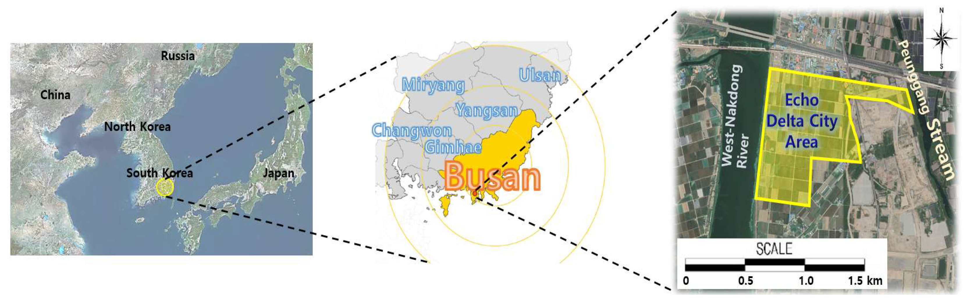
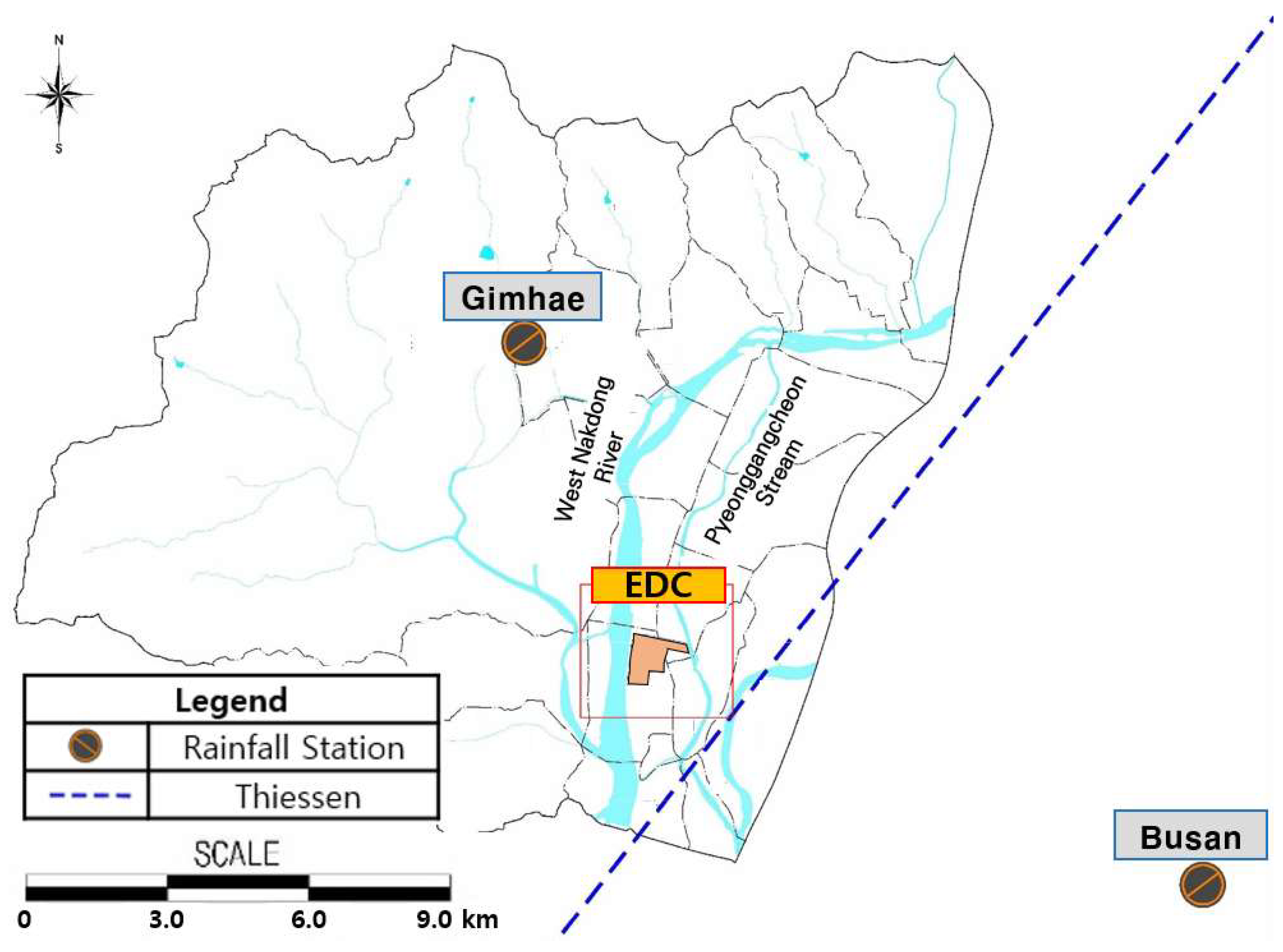
The watershed of the study area was the Eco-Delta City (EDC) located in Busan city in Korea. The location of the study area is shown in Figure 1. The total area was 105.9 ha (1.059 km²). The West Nakdong River on the west flows from north to south, and the Pyeonggangcheon Stream on the east flows into the West Nakdong River through the Suna sluice gate. The study area was the estuary of the West Nakdong River, which consists of flat land with an elevation of 50 m or less (mostly 0.4 to 4.0 m), and the difference in height between the river and the land is less than 1.0 m, being mostly lowlands. In addition, agricultural water is supplied to the existing irrigation channel in study area through the lower culvert of the Namhae Expressway, but it will be closed due to development of the study area, and there is no external inflow.

Therefore, the study area was selected with regard to the topographical condition of the area and the design stage before the installation of the LID facility, as well as the fact that the permeable pavement will have a large reduction effect on the flat land.

3.2. Collection of Hydrological Data

The rainfall station was selected according to the distance from the study area. Therefore, the Gimhae rainfall station was selected, as it is located close to Gimhae-si, with the data exceeding 30 years. The annual maximum daily rainfall data from the Gimhae rainfall station were used in this study [12]. The location of the Gimhae rainfall station is shown in Figure 2.

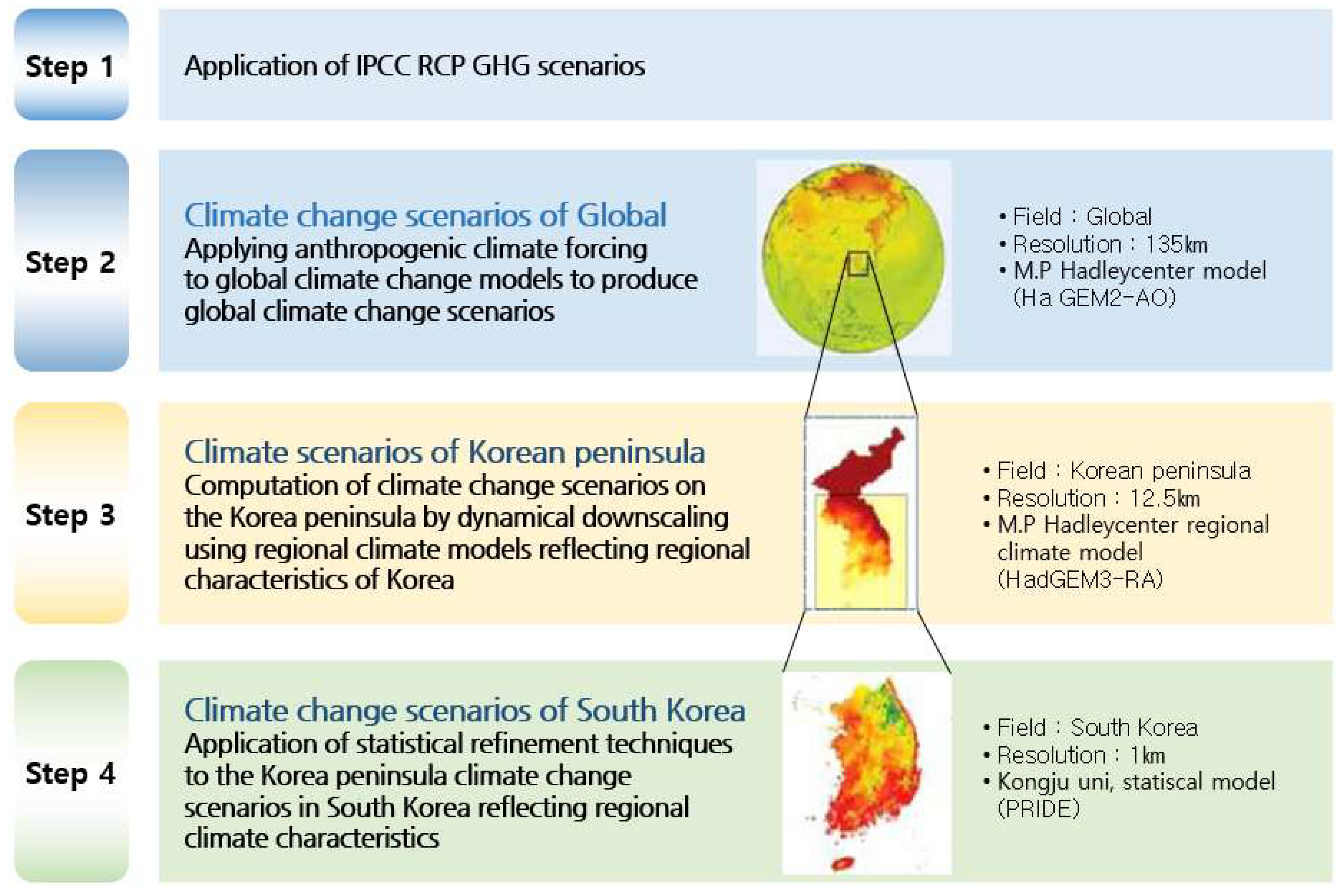
In addition, the Korean Peninsula climate change scenario was analyzed using the global climate change scenario data of the HadGEM2-AO model, and was developed in Korea using the HadGEM3-RA model (Hadley Center Global Environment Model version 3 atmosphere regional climate model) at a resolution of 12.5 km.

Production process for climate change scenarios is shown in Figure 3.

In this study, the RCP 4.5 scenario was simulated for the peninsula for 200 years with 12.5 km resolution, and the integral control was based on the RCP 8.5 scenario. The extraction of annual maximum daily rainfall data was based on the past observed time series of daily rainfall (1988–2018) and the climate change scenarios from 2019 to 2100.

The annual maximum daily rainfall for the next 100 years suitable for the EDC, the research study area, was analyzed and used as shown in

Table 1. Annual maximum daily rainfall according to climate change scenarios.

Year	RCP Scenarios		Year	RCP Scenarios		Year	RCP Scenarios
	RCP 4.5	RCP 8.5		RCP 4.5	RCP 8.5		RCP 4.5	RCP 8.5
1988	83.0	83.0	2026	145.0	205.8	2064	145.6	87.7
1989	296.0	296.0	2027	93.7	70.0	2065	128.2	106.6
1990	126.0	126.0	2028	134.0	117.3	2066	219.9	109.7
1991	218.0	218.0	2029	85.7	123.9	2067	98.7	65.7
1992	164.0	164.0	2030	117.0	68.0	2068	91.5	112.0
1993	140.0	140.0	2031	113.0	212.1	2069	84.9	101.5
1994	97.0	97.0	2032	50.9	95.4	2070	65.0	134.7
1995	93.0	93.0	2033	66.3	256.1	2071	116.5	91.9
1996	103.0	103.0	2034	189.7	94.0	2072	264.4	120.2
1997	119.0	119.0	2035	124.1	105.8	2073	157.4	187.8
1998	109.0	109.0	2036	168.7	108.7	2074	102.2	68.3
1999	131.0	131.0	2037	57.5	124.8	2075	79.0	71.7
2000	83.0	83.0	2038	82.4	83.4	2076	65.6	97.5
2001	73.0	73.0	2039	229.4	76.1	2077	83.8	163.5
2002	160.0	160.0	2040	85.2	121.6	2078	86.5	80.9
2003	108.0	108.0	2041	113.7	63.5	2079	129.5	82.2
2004	127.0	127.0	2042	133.6	71.9	2080	108.6	123.7
2005	179.0	179.0	2043	80.1	121.1	2081	95.4	128.6
2006	131.0	131.0	2044	130.2	82.7	2082	156.3	127.3
2007	100.0	100.0	2045	80.9	112.8	2083	116.7	171.2
2008	111.0	111.0	2046	216.8	131.9	2084	129.9	101.4
2009	218.0	218.0	2047	86.7	96.9	2085	249.0	89.2
2010	119.0	119.0	2048	156.3	82.0	2086	79.5	72.0
2011	189.0	189.0	2049	93.2	60.0	2087	107.5	122.0
2012	119.0	119.0	2050	110.4	69.1	2088	137.3	403.6
2013	102.0	102.0	2051	111.5	147.9	2089	79.9	83.3
2014	238.0	238.0	2052	157.8	334.9	2090	75.2	97.9
2015	53.0	53.0	2053	176.7	111.8	2091	162.3	81.1
2016	140.0	140.0	2054	114.2	113.3	2092	112.9	269.1
2017	168.0	168.0	2055	140.5	162.6	2093	69.2	142.0
2018	88.0	88.0	2056	99.1	63.4	2094	150.4	121.1
2019	88.9	121.8	2057	355.9	105.8	2095	152.4	124.4
2020	121.1	81.9	2058	108.3	101.7	2096	123.0	141.5
2021	157.2	151.2	2059	189.6	69.5	2097	96.4	181.9
2022	131.6	85.5	2060	75.3	91.7	2098	132.4	151.2
2023	133.2	97.4	2061	152.4	110.9	2099	100.3	105.6
2024	84.7	85.2	2062	81.2	87.0	2100	65.7	74.6
2025	127.6	73.9	2063	103.8	104.6

.

3.3. Input Data Composition of SWMM Model

The parameters of the SWMM model are watershed area, permeability, Manning’s roughness coefficients, surface storage volume, storage depth, CN value, slope, and sewage pipe data. The rainfall runoff is simulated using these parameters as input data. However, since there is limited observation data to apply all parameters, in this study, watershed area, permeability, Manning’s roughness coefficients, slope, and sewage pipe data were used as parameters.

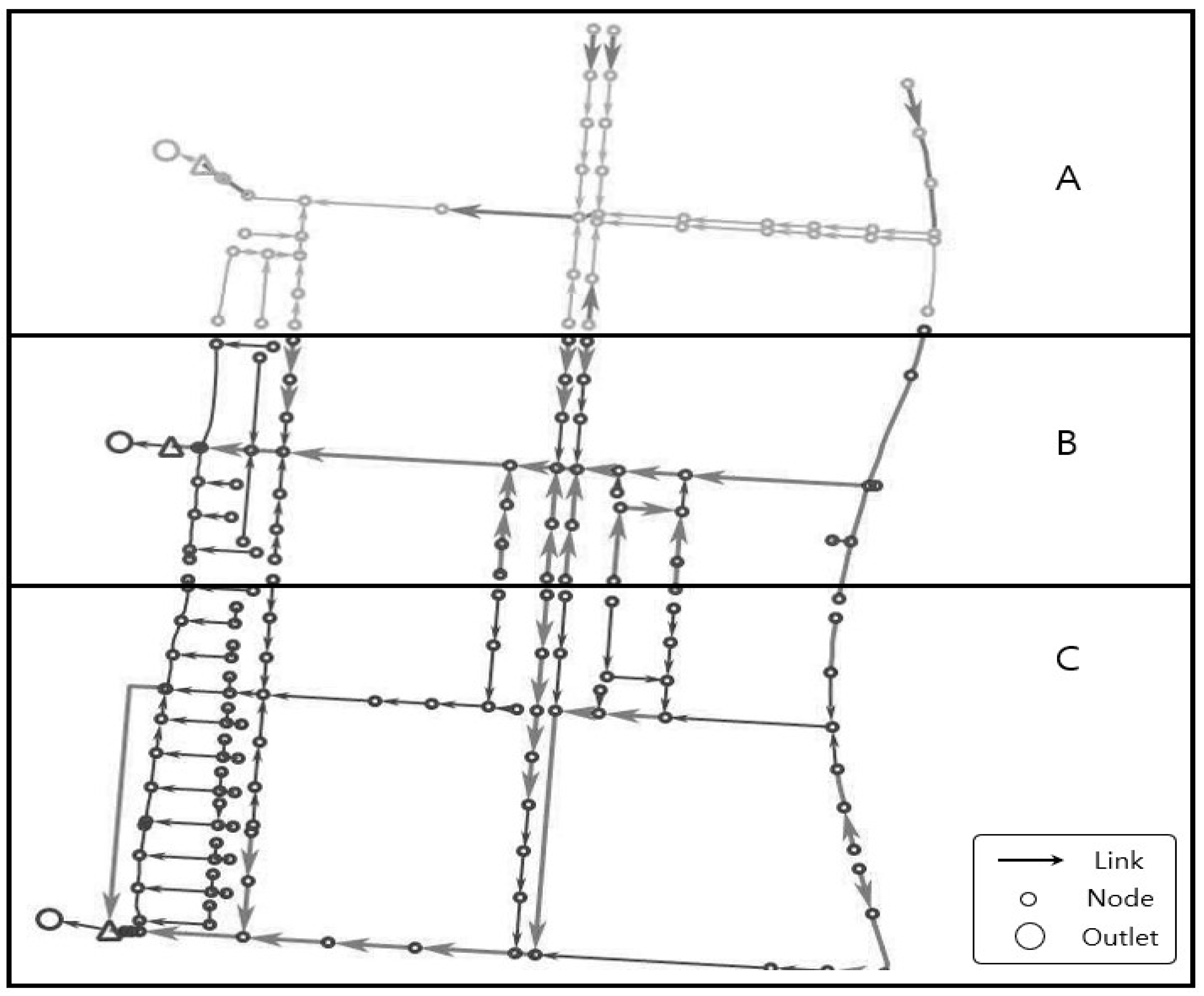
In Korea, the EPA-SWMM is used for flood analysis of LID facilities, and in the case of LID facility effect analysis, the most accurate and ideal result is obtained by performing monitoring under the same conditions before and after installation of the facility and analyzing the effect. In this section, the parameters and data construction before and after LID facility installation are presented. Watershed delineation is the first step in simulating the physical drainage systems. In the EPA-SWMM model, the subwatershed is assumed to be a rectangle with uniform characteristics (slope, roughness, etc.). The shape of the watershed is defined by factors such as area, watershed width, slope, etc. In the case of the EDC area, it flows out through three outlets, and in the case of each watershed, the model was built by unifying the watershed names A, B, and C, as shown in Figure 4, with all three watersheds flowing into the West Nakdong River. The watersheds were divided into subwatersheds according to the pipe network, and there were 133 subwatersheds in A, 171 in B, and 202 in C. The pipe network, according to watershed area, subwatersheds, outlets, nodes, and links, is presented in

Table 2. Pipe network.

Watershed Area (ha)		Subwatershed (pcs)	Outlet (pcs)	Node (pcs)	Link (pcs)
A	29.4	133	1	43	43
B	32.4	171	1	52	52
C	44.1	202	1	93	93
Total	105.9	506	3	188	188

and Figure 4.

To introduce the LID facilities, variables for each facility were applied.

Table 3. Parameter values of permeable pavement.

Division		Attribute Value
Surface	Berm height (mm)	0
	Vegetation volume fraction	0
	Surface roughness (Manning n)	0.012
	Surface slope (%)	1
Pavement	Thickness (mm)	60
	Void ratio (Voids/Solids)	0.15
	Impervious surface fraction	0.95
	Permeability (mm/h)	360
	Clogging factor	0
Storage	Height (mm)	300
	Void ratio (Voids/Solids)	0.25
	Conductivity (mm/h)	25.9
	Clogging factor	0
Underdrain	Drain coefficient (mm/h)	0
	Drain exponent	0
	Drain offset height	0

In addition, the drainage area of EDC is 52.95 ha, which is 50% of the total watershed area of 105.90 ha. The roughness coefficients among the conduit input data, 0.030 for the permeable area and 0.014 for the impervious area, were applied.

shows the designated values of the permeable pavement in this study.

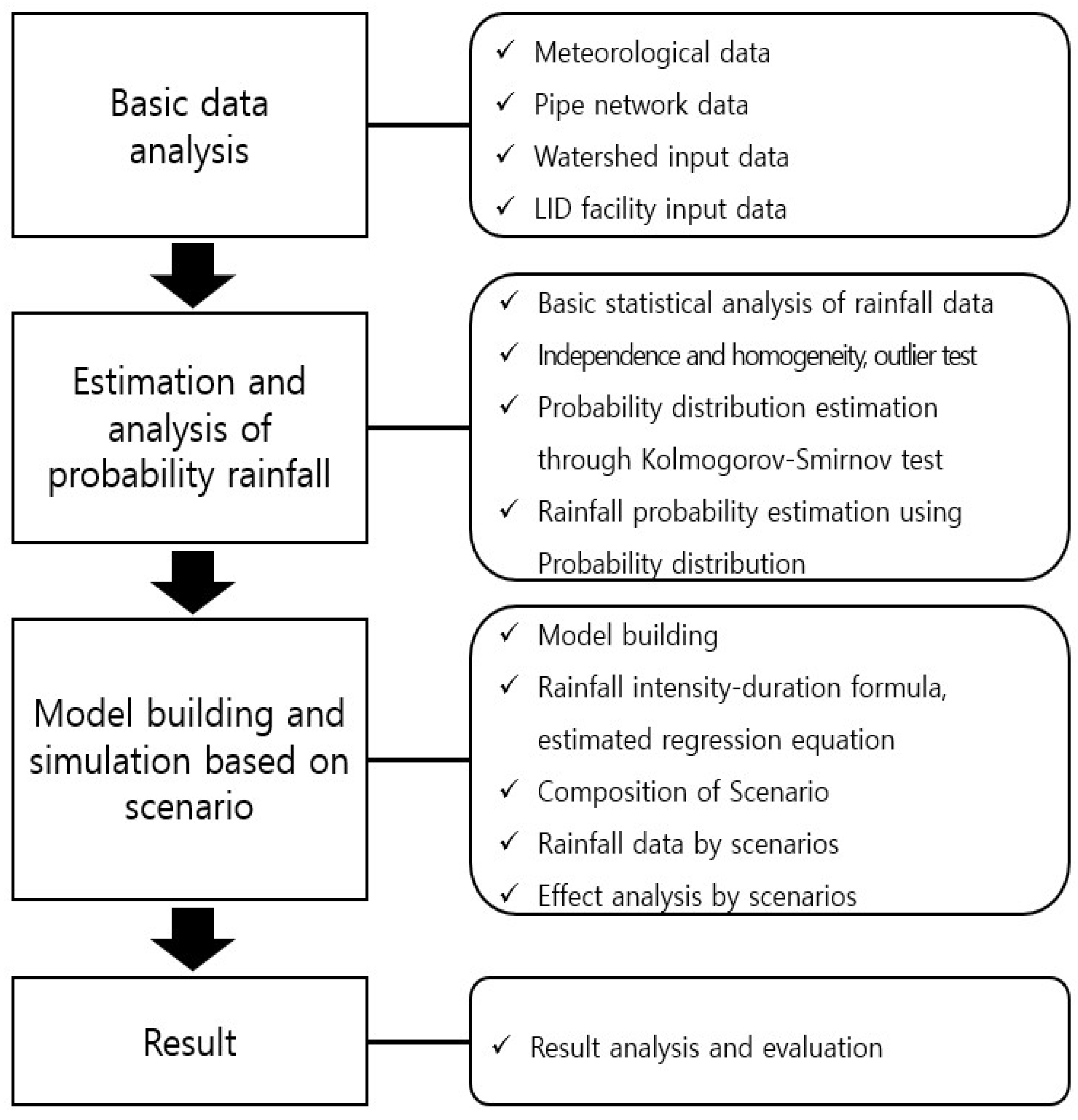
3.4. Research Methodology

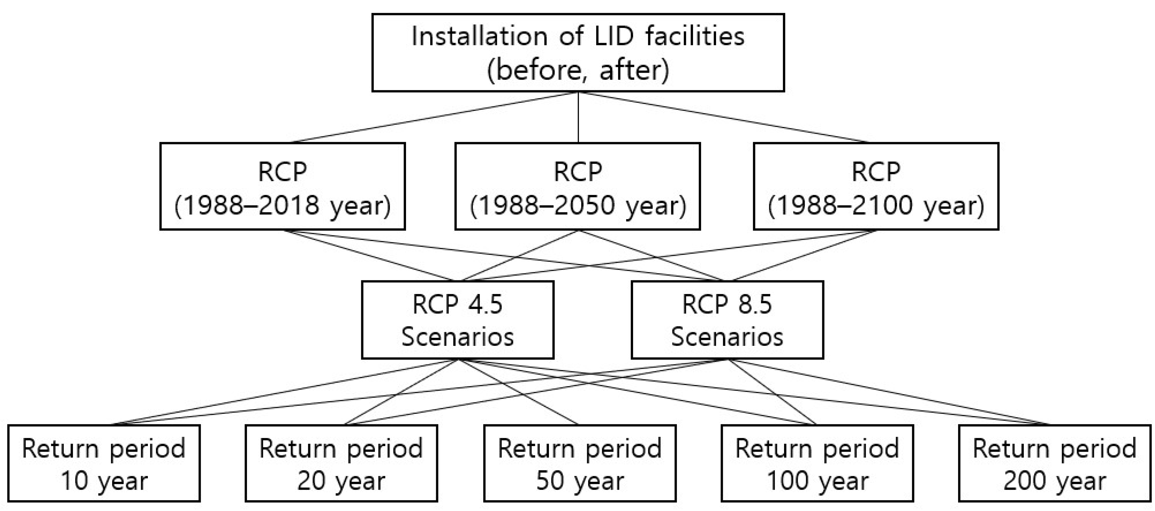
The following procedure was followed to analyze the reduction rate of the runoff of the LID facility installed in selected watersheds.

The extraction of annual maximum daily rainfall data was based on the past observed time series of daily rainfall (1988–2018) and the climate change scenarios from 1988 to 2050 and 1988 to 2100. The statistical tests, such as the mean, standard deviation, coefficient of variation, coefficient of skewness, and coefficient of kurtosis, were applied to hydrological data. After calculating the basic statistical values of the annual maximum daily rainfall series, the time series were tested for independence, homogeneity, and outliers. An appropriate distribution was selected for the GUM, PT3, GEV, GLO, GPA, and GNO distributions through the goodness-of-fit test. The parameters of the appropriate distribution were computed according to the study area and the period of analysis using the L-moment method, and the probability of rainfall was estimated using the selected appropriate distribution. Probability of rainfall was computed according to the climate change scenarios.

A rainfall intensity duration equation was derived, and the regression equation was calculated using the precipitation data from the selected rainfall station. The rainfall distribution of the probability of rainfall was constructed using the calculated regression equation. In the EPA-SWMM, the same pipe network data, parameters, and rainfall data before and after the installation of the LID facility were established, and the parameters for the facility after the installation of the LID facility were additionally configured. The effect analysis was presented by estimating the probability of rainfall for each return period of climate change scenario, such as RCP 4.5 and RCP 8.5, by simulating runoff and comparing the reduction rate.

Figure 5 is a schematic diagram of the probability precipitation calculation considering climate change scenarios and LID facilities. The flow chart used in the study based on the procedure introduced in Figure 5 is shown in Figure 6.

4. Results

4.1. Basic Statistical Analysis and Calculation of Probable Rainfall According to Climate Change Scenario

The mean, standard deviation, coefficient of skewness, coefficient of variation, and coefficient of kurtosis for the annual maximum daily rainfall data from the Gimhae rainfall station were calculated. The mean and standard deviation for each period of the RCP 4.5 scenario ranged from 126.2 m³/day to 135.0 m³/day and 48.502 to 53.361, respectively, the coefficient of skewness and coefficient of variation were from 1.162 to 1.618 and 0.383 to 0.408, respectively, and the coefficient of kurtosis was from 1.616 to 3.769. This indicated overall that the mean was larger than the range of standard deviation, the coefficient of skewness and the coefficient of variation showed positive values and were biased to the right, and the coefficient of kurtosis was larger than 3, the standard value of normal distribution.

In the RCP 8.5 scenario, the mean and standard deviation ranged from 121.2 to 135.0 and 50.727 to 56.491, respectively, the coefficient of skewness and the coefficient of variation were from 1.231 to 2.255 and 0.395 to 0.461, respectively, and the coefficient of kurtosis was from 1.616 to 6.828.

The basic statistics for RCP 4.5 and RCP 8.5 are shown in

Table 4. Basic statistics for Gimhae rainfall station using RCP 4.5 scenario.

Duration of Observed Data (Years)	Mean ( $\overline{\mathit{x}}$) (m3/s)	Standard Deviation (S)	Coefficient of Skewness $\left({\mathit{C}}_{\mathit{s}}\right)$	Coefficient of Variation $\left({\mathit{C}}_{\mathit{v}}\right)$	Coefficient of Kurtosis (CA)
1988–2018	135.0	53.361	1.231	0.395	1.616
1988–2050	126.6	48.502	1.162	0.383	1.646
1988–2100	126.2	51.428	1.618	0.408	3.769

and

Table 5. Basic statistics for Gimhae rainfall station using RCP 8.5 scenario.

Duration of Observed Data (Years)	Mean ( $\overline{\mathit{x}}$) (m3/s)	Standard Deviation (S)	Coefficient of Skewness $\left({\mathit{C}}_{\mathit{s}}\right)$	Coefficient of Variation $\left({\mathit{C}}_{\mathit{v}}\right)$	Coefficient of Kurtosis (CA)
1988–2018	135.0	53.361	1.231	0.395	1.616
1988–2050	121.2	50.727	1.421	0.418	1.947
1988–2100	122.4	56.491	2.255	0.461	6.828

.

4.2. Independence, Homogeneity, and Outlier Detection in Annual Maximum Daily Rainfall

The climate change scenario data were checked to determine the existence of independence, homogeneity, and outliers. The Wald–Wolfowitz test was applied to check the independence, and the Mann–Whitney test was applied to observe the homogeneity of the data. In addition, the Grubbs–Beck test was used for the detection of outliers in the time series data.

For the independence test, the Wald–Wolfowitz test [14], which is a non-parametric test that tests the independence of a population, was performed, and it was found that there were no abnormalities in any of them.

The outlier test induces inappropriate statistical parameters in the case of data that appear far above or below the general balanced distribution of hydrological data, resulting in uncertainty in the presentation of the design hydrologic quantity. Therefore, the presence or absence of outliers was tested using the Grubbs–Beck method for hydrological data of the daily maximum flow series for each analysis in the region to which the climate change scenario was applied. It was confirmed that there were no outliers.

Therefore, the annual maximum daily rainfall in the study area was recognized as valid for analysis as hydrological data.

4.3. Estimation of L-Moment Ratio

L-moment ratios were estimated for goodness-of-fit test evaluation of the probability distributions, such as GUM, PT3, GEV, GLO, GPA, and GNO. L-skewness and L-kurtosis were calculated for the 1988–2018, 1988–2050, and 1988–2100 periods using the annual maximum daily rainfall of RCP 4.5 and RCP 8.5.

In the case of RCP 4.5, L-skewness was 0.2535, 0.2136, and 0.2510, and L-kurtosis was 0.2108, 0.1884, and 0.1999. In the case of RCP 8.5, L-skewness was 0.2535, 0.2822, and 0.3321, and L -kurtosis was 0.2108, 0.2019, and 0.2538.

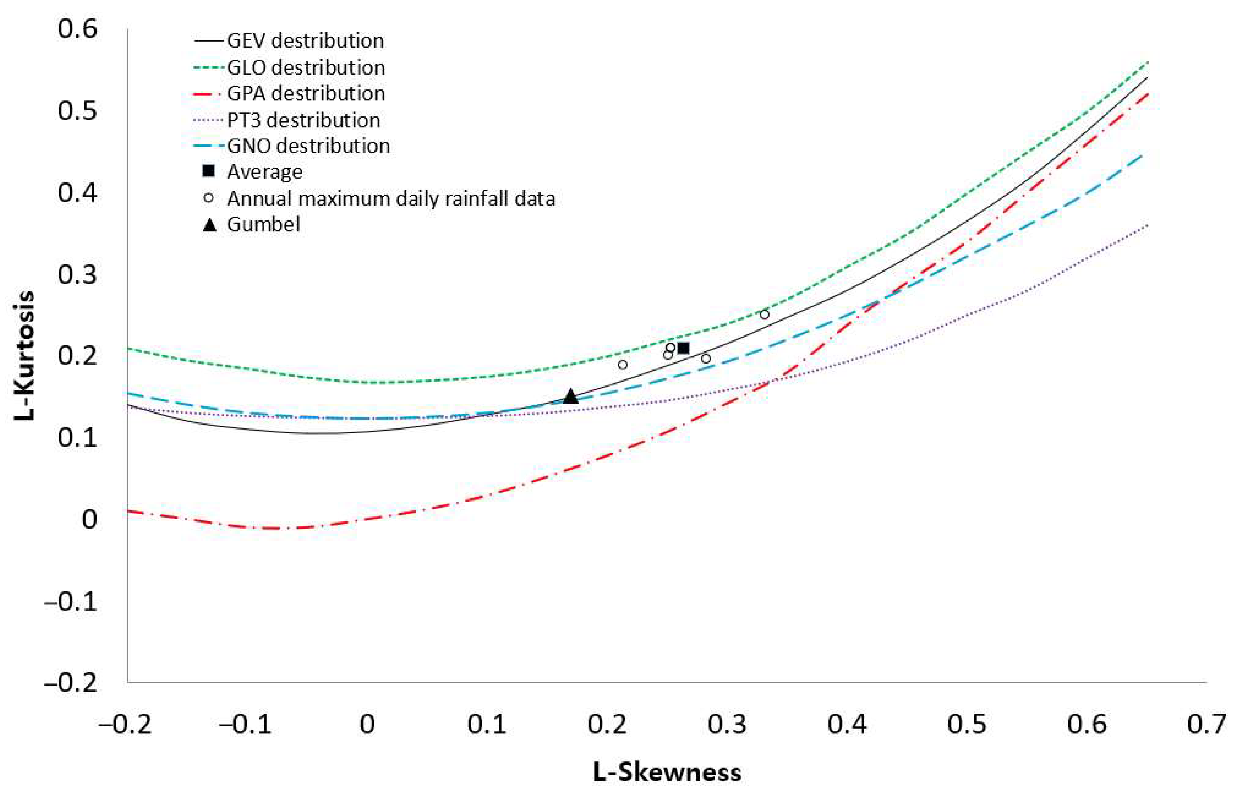
4.4. Goodness-of-Fit Test

For the goodness-of-fit test, L-moment ratio and Kolmogorov–Smirnov (K–S) tests were performed. First, the selection of an appropriate probability distribution for each period was made by plotting the L-moment ratio, using the L-moment ratio calculated in the previous section. The L-moment ratio diagram was plotted to select the best fitted probability distribution from among GUM, PT3, GEV, GLO, GPA, and GNO. The best fitted probability distribution is the one that follows the observed data.

Therefore, Figure 7 shows the average values of the L-moment ratio for the RCP 4.5 and RCP 8.5 scenarios.

The dimensionless L-moment ratios scattered in the diagram are more likely to follow the curve of the GEV distribution, as shown in Figure 7. Therefore, the L-moment method application on the annual maximum daily rainfall for each rainfall station and its plotting in the L-moment ratio diagram showed that the GEV distribution was an appropriate probability distribution compared with GUM, GLO, GPA, GNO and PT3.

Second, the K–S test was applied to choose the best fitted probability distribution for each period of the annual maximum daily rainfall series of the climate change scenario. As a result, at the 5% significance level, data for each period of the annual maximum daily rainfall series were recognized as following the distribution of GEV, GUM, GLO, GPA, GNO, and PT3.

The L-moment ratio diagram and the K–S goodness-of-fit tests showed that the GEV distribution was best fitted probability distribution compared with the other probability distributions. Therefore, the GEV distribution was selected for further analysis.

4.5. Parameter Estimation of Desired Distribution According to L-Moment Method

The parameters of the GEV distribution were estimated by applying it to the annual maximum daily rainfall of the climate change scenarios of RCP 4.5 and RCP 8.5. The parameters of the GEV distribution consist of shape, scale, and location, estimated using the L-moment method for defined periods. The parameters of the GEV distribution that were estimated for the RCP 4.5 and RCP 8.5 scenarios are shown in

Table 6. Parameters calculated by GEV distribution using L-moment method considering RCP 4.5 scenario at Gimhae rainfall station.

Duration of Observed Data (Years)	Parameter
	$\mathit{\xi }$	$\mathit{\alpha }$	$\mathit{\beta }$
1988–2018	108.2442	96.9893	−0.1260
1988–2050	103.4955	35.6241	−0.0668
1988–2100	101.8388	34.1054	−0.1224

and

Table 7. Parameters calculated by GEV distribution using L-moment method considering RCP 8.5 scenario at Gimhae rainfall station.

Duration of Observed Data (Years)	Parameter
	$\mathit{\xi }$	$\mathit{\alpha }$	$\mathit{\beta }$
1988–2018	108.4242	96.9893	−0.1260
1988–2050	96.2268	32.2964	−0.1675
1988–2100	95.8663	30.1751	−0.2377

.

4.6. Computation of Return Periods Based on Annual Maximum Daily Rainfall

Return periods were computed through the application of GEV distribution on annual maximum daily rainfall of the climate change scenario using the parameters computed in the section above, as shown in

Table 8. Probable annual maximum daily rainfall at Gimhae rainfall station using RCP 4.5 scenario (unit: mm/day).

Duration of Observed Data (Years)	Return Period (Years)
	10	20	50	100	200
1988–2018	204.66	241.67	294.83	338.97	386.98
1988–2050	190.00	220.54	262.30	295.35	329.85
1988–2100	190.20	224.00	272.41	312.49	355.98

and

Table 9. Probable annual maximum daily rainfall at Gimhae rainfall station using RCP 8.5 scenario (unit: mm/day).

Duration of Observed Data (Years)	Return Period (Years)
	10	20	50	100	200
1988–2018	204.66	241.67	294.83	338.97	386.98
1988–2050	184.50	220.51	274.07	320.05	371.53
1988–2100	185.65	226.10	289.85	347.79	415.92

.

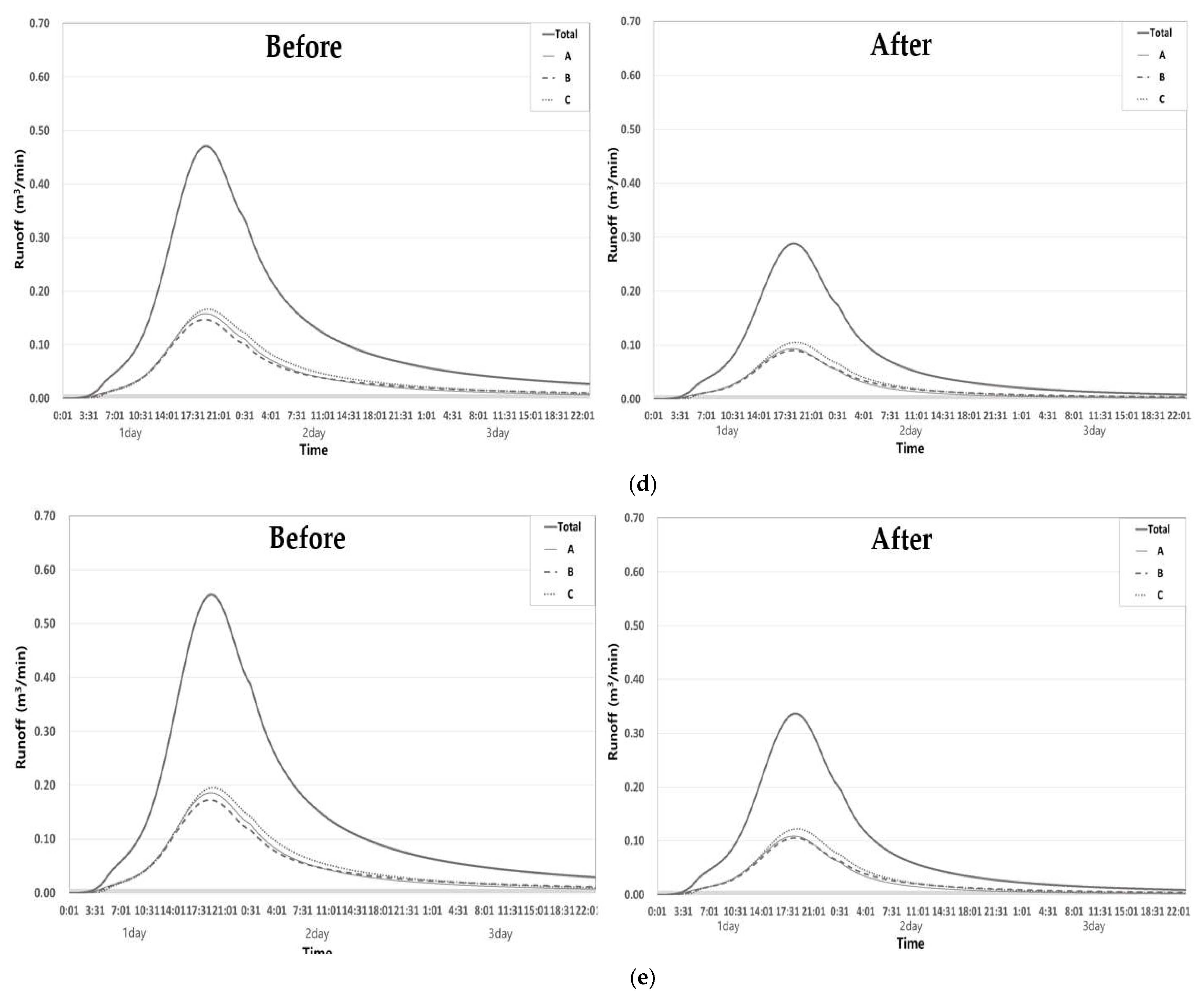
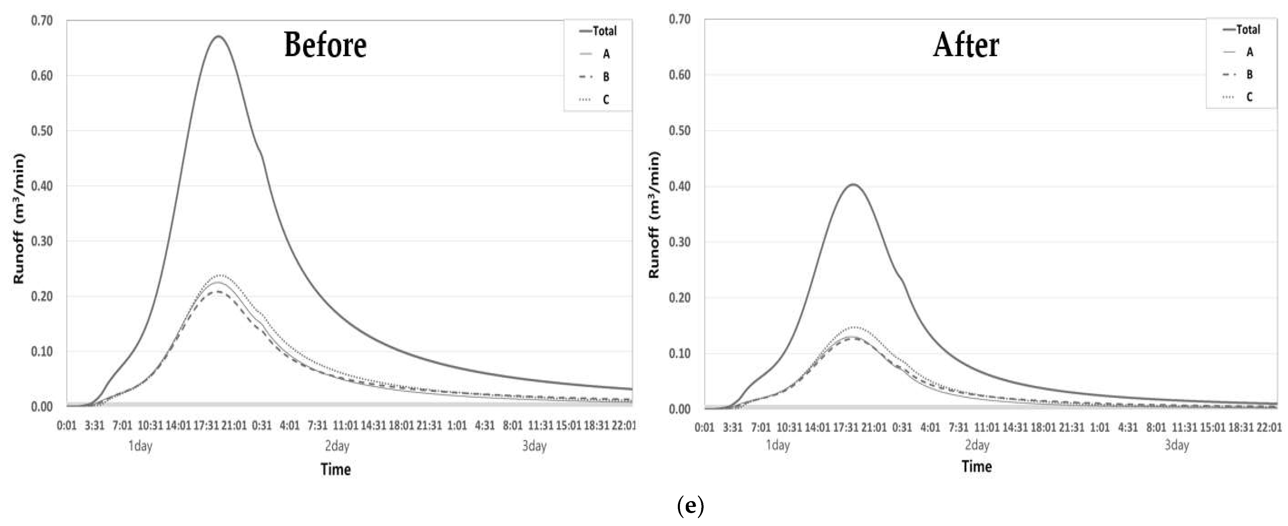
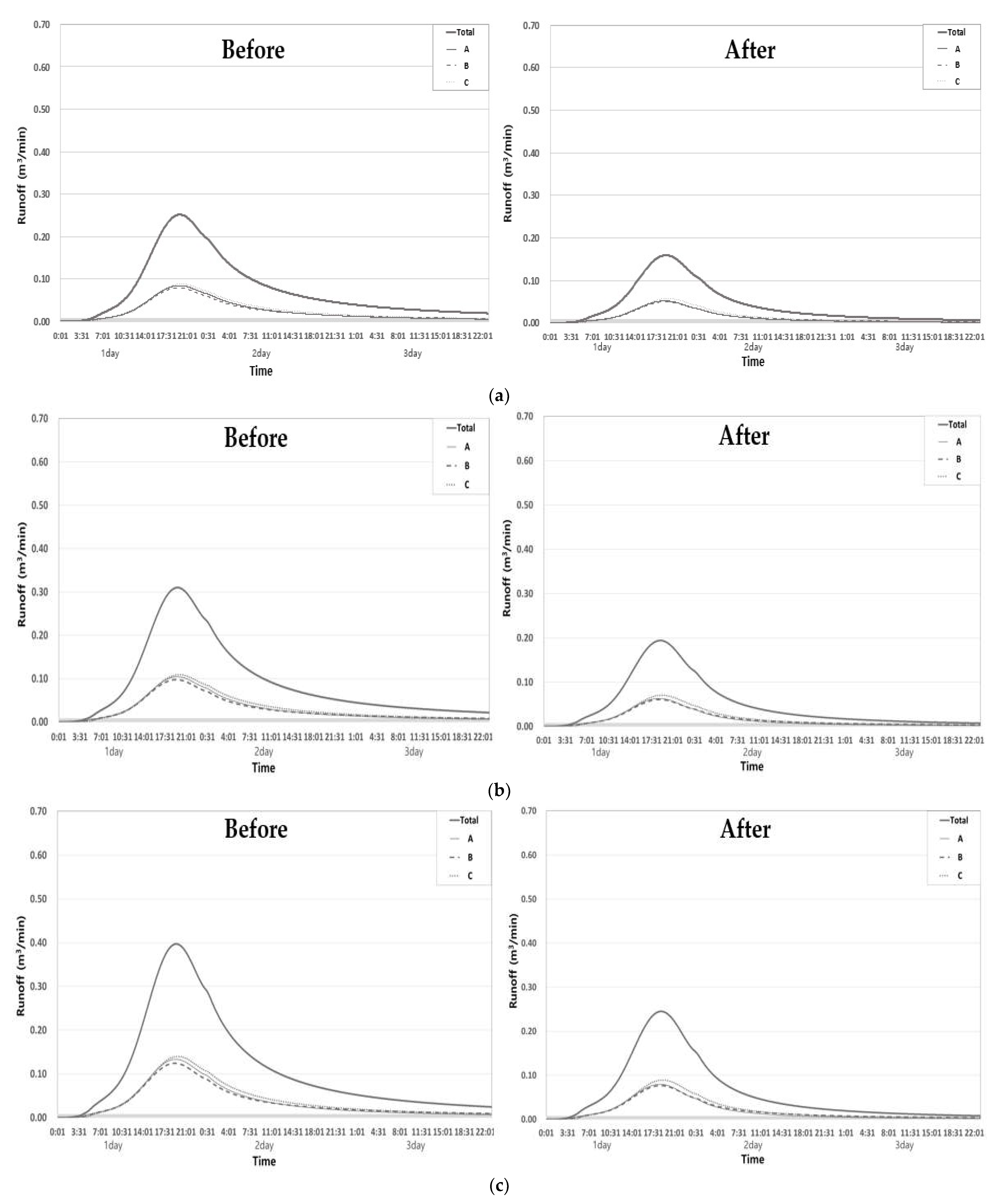
4.7. Analysis of Runoff before and after Application of LID Facilities by Climate Change Scenario

As a result of the analysis of the reduction rate for RCP 4.5 and RCP 8.5 during the 1988–2018 period, it was found that the reduction rate for the total amount of runoff increases as the return period increases.

In addition, as a result of the analysis of the reduction rate from 1988 to 2050 for the RCP 4.5 scenario, the 10-year return period was 45.4%, the 20-year return period was 45.8%, the 50-year return period was 46.2%, the 100-year return period was 46.5%, and the 200-year return period was 46.7%. It was found that the greater the return period, the greater the reduction rate.

Analyzing the RCP 4.5 scenario as a sample, the reduction rate from 1988 to 2100 decreased from 321.8 m³/day to 175.7 m³/day in the 10-year return period of the total runoff, showing a reduction rate of 45.4%. In the 20-year return period, it decreased from 386.8 m³/day to 209.6 m³/day, showing a reduction rate of 45.8%; and in the 50-year return period, it decreased from 481.1 m³/day to 258.4 m³/day, showing a reduction rate of 46.3%. In the case of the 100-year return period, it decreased from 559.9 m³/day to 299.0 m³/day, a reduction rate of 46.6%; and in the 200-year return period, it decreased from 646.2 m³/day to 343.3 m³/day, showing a reduction rate of 46.9%.

Table 10. Runoff and reduction rate by return period of maximum daily rainfall (RCP 4.5, 1988–2100).

Return Period (Years)	Watershed Area	Peak Rate of Runoff (m3/s)		Reduction Efficiency (%)	Runoff (m3/Day)		Reduction Efficiency (%)
		Before	After		Before	After
10	A	0.084	0.052	38.5	105.2	54.6	48.1
	B	0.079	0.050	37.1	101.4	57.4	43.4
	C	0.088	0.058	34.6	115.2	63.7	44.7
	Total	0.252	0.159	36.7	321.8	175.7	45.4
20	A	0.104	0.063	39.4	126.0	64.9	48.5
	B	0.097	0.061	37.7	122.2	68.7	43.8
	C	0.109	0.070	35.4	138.5	76.0	45.2
	Total	0.310	0.194	37.4	386.8	209.6	45.8
50	A	0.133	0.080	40.3	156.1	79.7	49.0
	B	0.124	0.077	38.3	152.6	85.1	44.2
	C	0.140	0.089	36.3	172.3	93.6	45.7
	Total	0.397	0.245	38.3	481.1	258.4	46.3
100	A	0.158	0.093	41.0	181.2	92.0	49.2
	B	0.147	0.090	38.7	178.2	98.8	44.5
	C	0.166	0.105	36.9	200.6	108.2	46.0
	Total	0.471	0.288	38.8	559.9	299.0	46.6
200	A	0.186	0.101	45.7	208.6	105.4	49.5
	B	0.172	0.105	39.0	206.2	113.7	44.8
	C	0.196	0.122	37.5	231.4	124.2	46.3
	Total	0.554	0.329	40.6	646.2	343.3	46.9

and Figure 8 show the results of the runoff and reduction rates according to the maximum daily rainfall by return period for the 1988–2100 period analysis of the RCP 4.5 scenario.

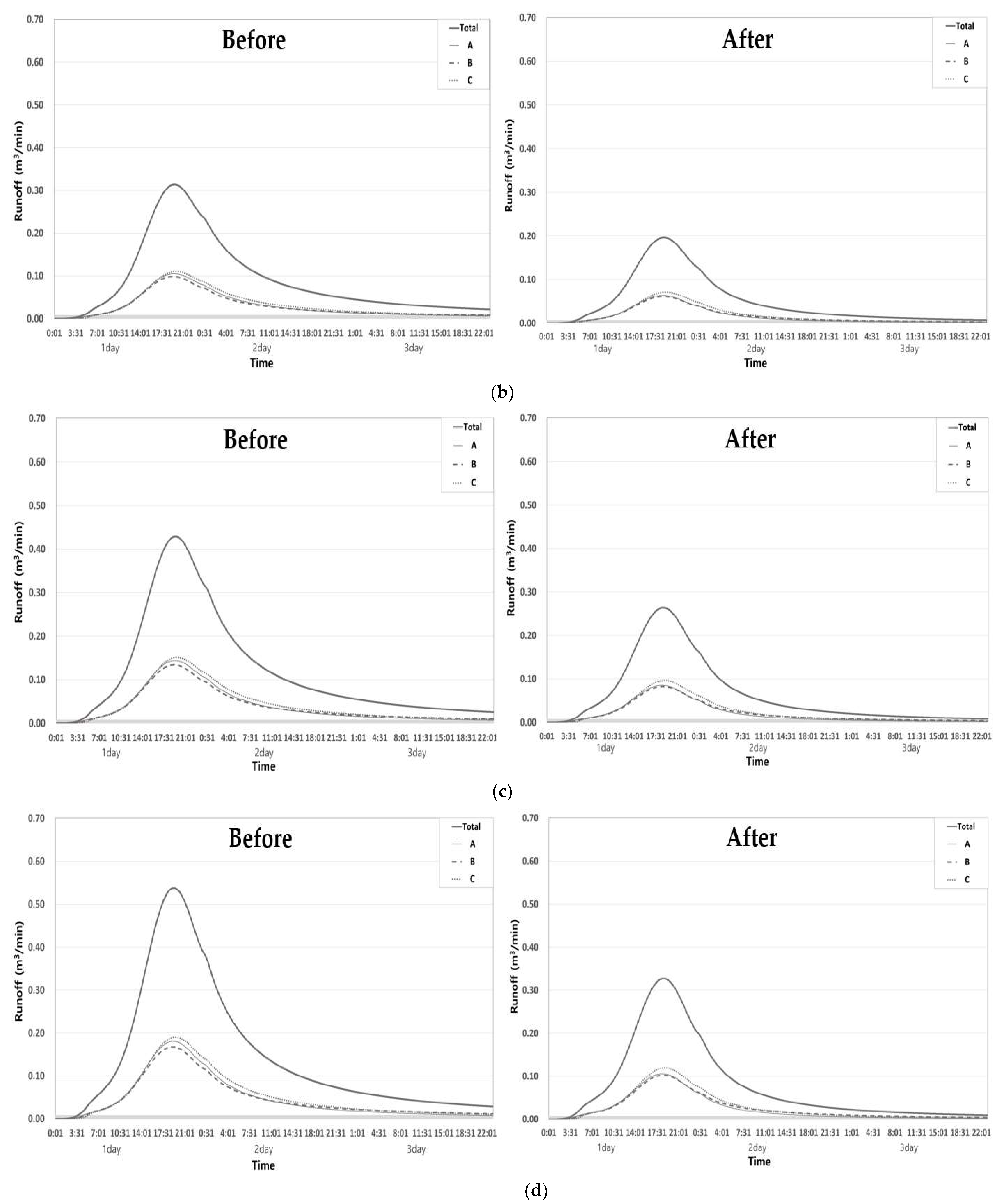
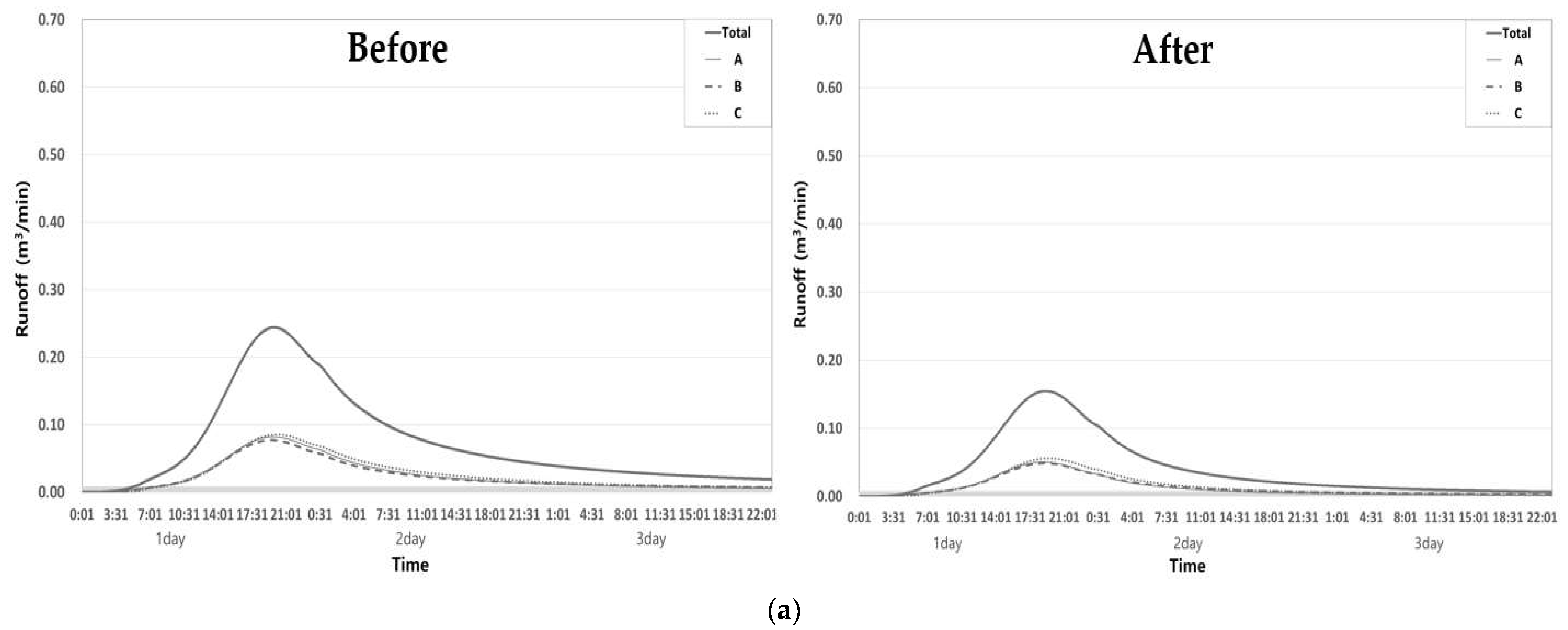
As a result of the analysis of the reduction rate for the RCP 8.5 scenario analysis from 2018 to 2050, the 200-year return period decreased from 677.2 m³/day of the total runoff to 359.1 m³/day, indicating the largest reduction rate of 47.0%.

Analyzing the RCP 8.5 scenario as a sample, the reduction rate from 1988 to 2100, during the RCP 8.5 scenario analysis period, for the 10-year return period of the total runoff decreased from 313.1 m³/day to 171.2 m³/day, showing a reduction rate of 45.3%. In the 20-year return period, it decreased from 390.8 m³/day to 211.7 m³/day, showing a reduction rate of 45.8%; and in the 50-year return period, it decreased from 515.3 m³/day to 276.0 m³/day, showing a reduction rate of 46.4%. In the case of the 100-year return period, it decreased from 629.9 m³/day to 334.9 m³/day, a reduction rate of 46.8%; and in the 200-year return period, it decreased from 766.1 m³/day to 404.5 m³/day, showing a reduction rate of 47.2%.

Table 11. Runoff and reduction rate by return period of maximum daily rainfall (RCP 8.5, 1988–2100).

Return Period (Years)	Watershed Area	Peak Rate of Runoff (m3/s)		Reduction Efficiency (%)	Runoff (m3/day)		Reduction Efficiency (%)
		Before	After		Before	After
10	A	0.082	0.050	38.4	102.4	53.2	48.1
	B	0.077	0.048	37.0	98.6	55.9	43.3
	C	0.085	0.056	34.5	112.1	62.1	44.6
	Total	0.244	0.155	36.6	313.1	171.2	45.3
20	A	0.105	0.064	39.4	127.3	65.5	48.5
	B	0.099	0.061	37.7	123.5	69.4	43.8
	C	0.110	0.071	35.4	140.0	76.7	45.2
	Total	0.314	0.196	37.5	390.8	211.7	45.8
50	A	0.144	0.086	40.6	167.0	85.1	49.1
	B	0.134	0.083	38.5	163.7	91.0	44.4
	C	0.151	0.096	36.6	184.6	99.9	45.9
	Total	0.429	0.264	38.5	515.3	276.0	46.4
100	A	0.181	0.106	41.4	203.4	102.9	49.4
	B	0.168	0.102	39.0	200.9	110.9	44.8
	C	0.190	0.119	37.4	225.6	121.2	46.3
	Total	0.538	0.327	39.3	629.9	334.9	46.8
200	A	0.225	0.130	42.2	246.5	123.8	49.8
	B	0.208	0.126	39.4	245.3	134.5	45.2
	C	0.238	0.147	38.2	274.2	146.2	46.7
	Total	0.671	0.403	39.9	766.1	404.5	47.2

and Figure 9 show the results for the runoff and reduction rates according to the maximum daily rainfall by return period for the 1988–2100 period analysis of the RCP 8.5 scenario.

4.8. Analysis of Reduction Rate by Climate Change Scenario

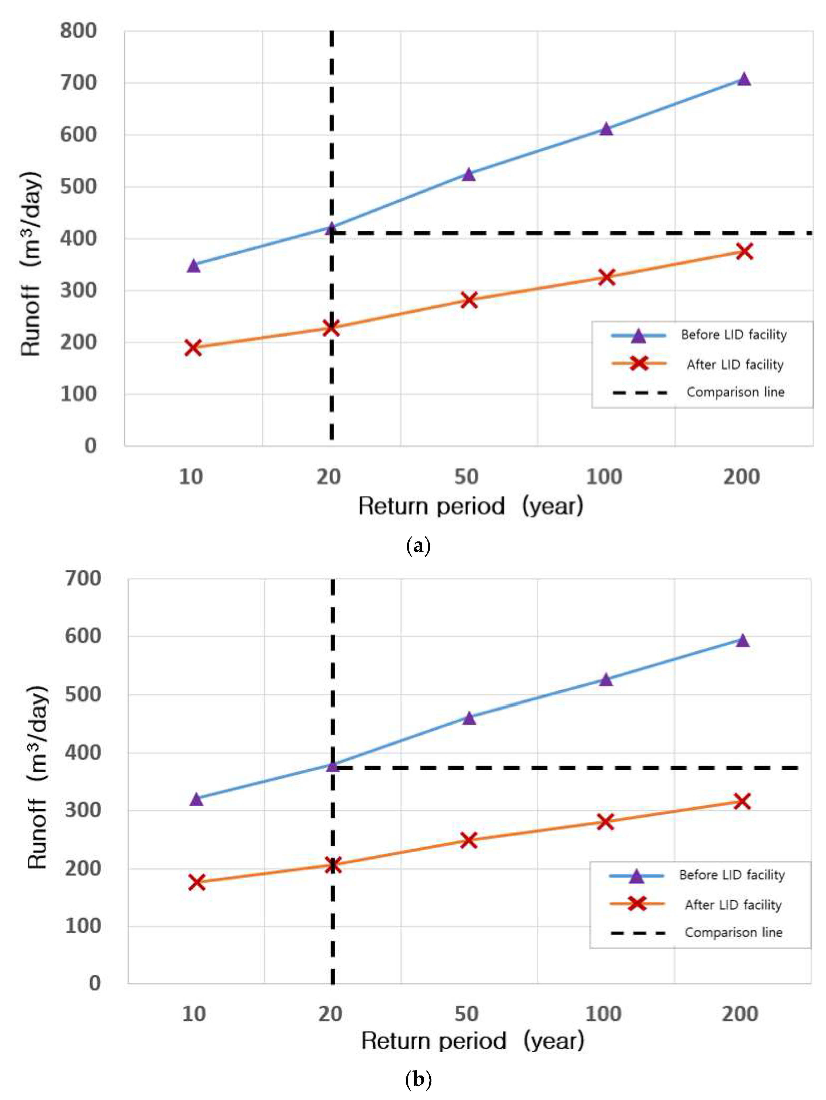
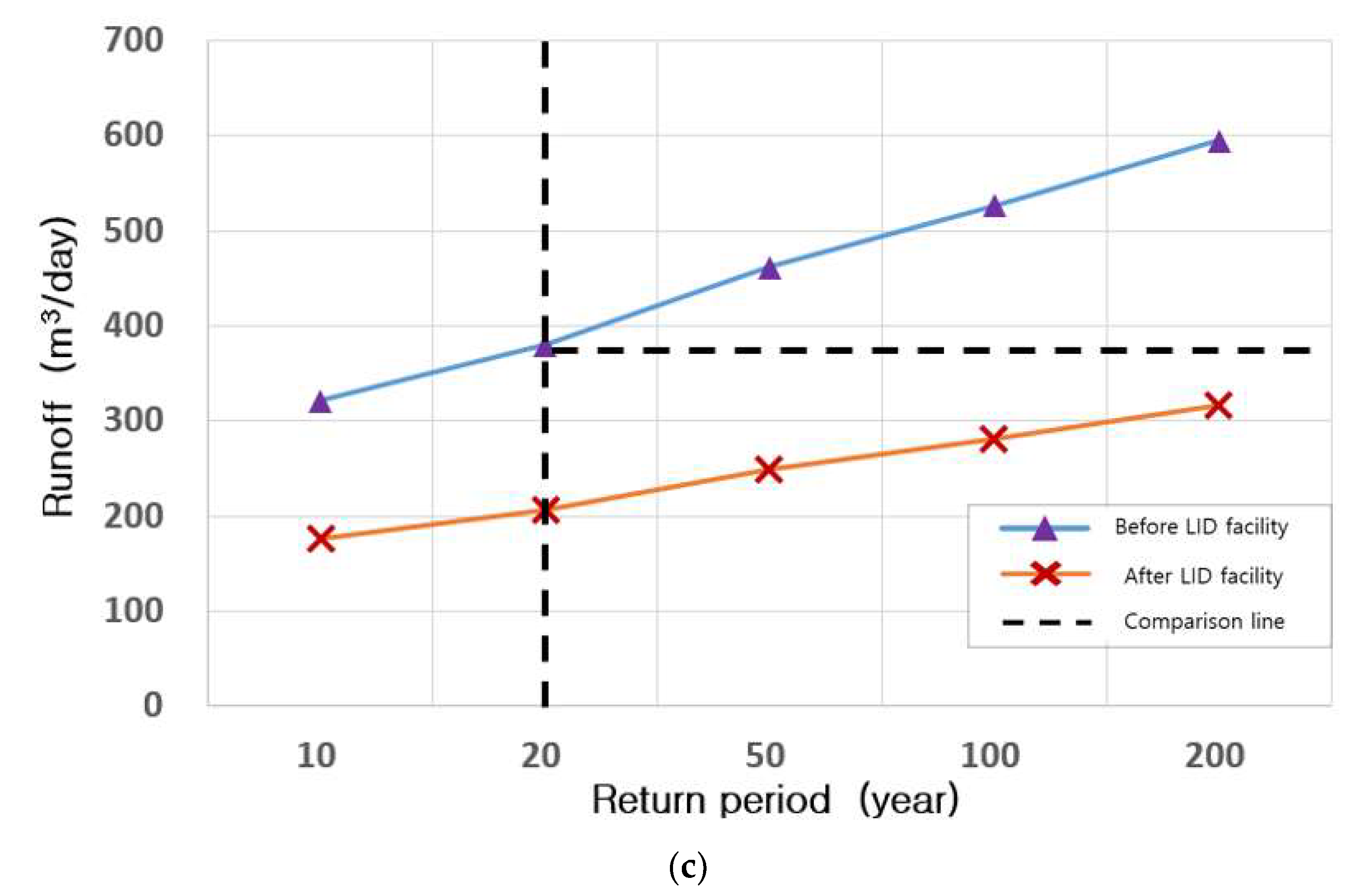
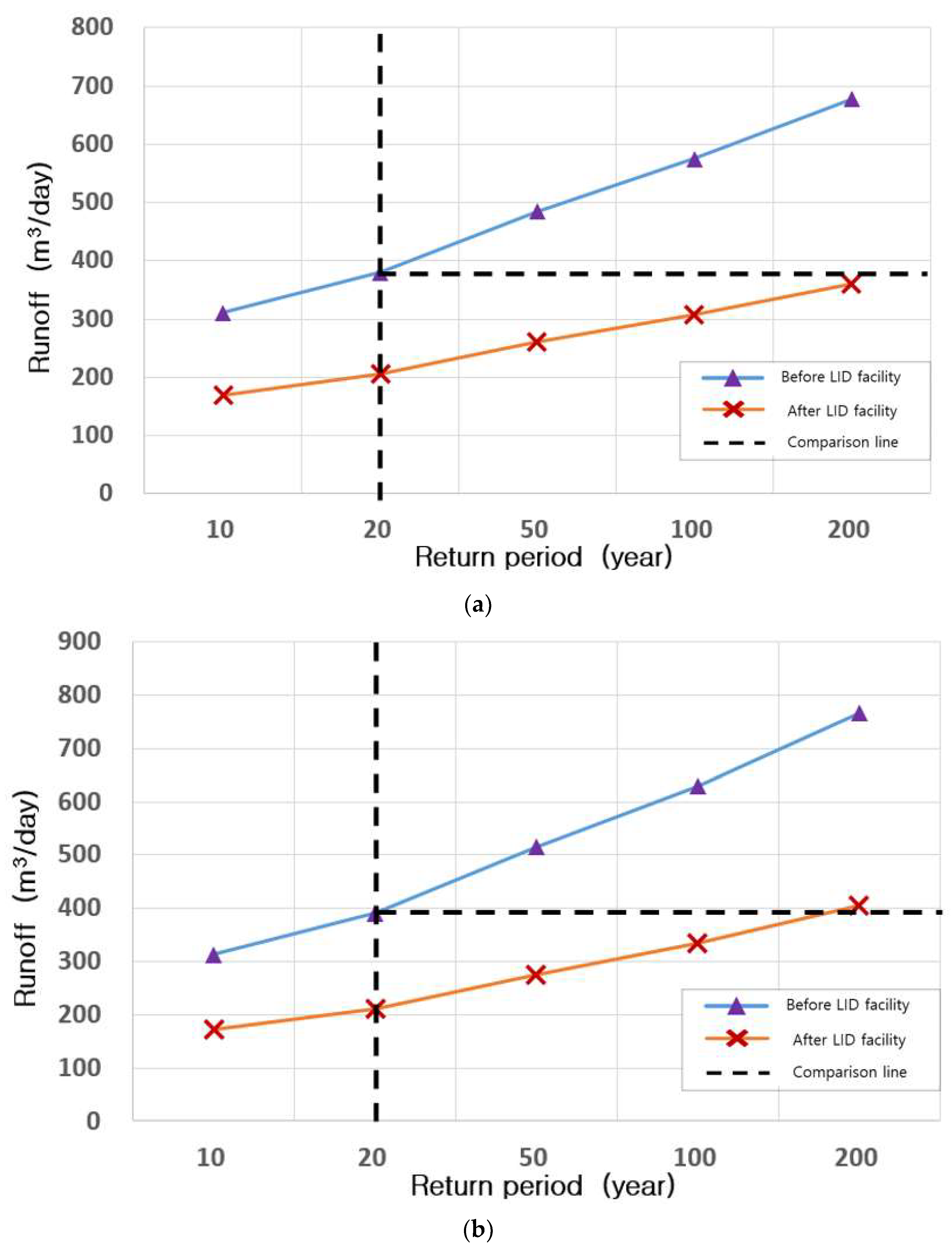
To efficiently manage runoff, it is necessary to determine the rainfall (design rainfall) to estimate the size of the reduction potential facility. A pre-disaster impact assessment is recommended [15]. The usual return period used in the design of temporary and permanent facilities is 30 and 50 years, respectively. As a result, a reduction rate return period analysis based on the 20-year runoff was reported in this study for LID facilities. The return period analysis from 1988 to 2018 was the same for the RCP 4.5 and RCP 8.5 scenarios; hence, it is reported only for the RCP 4.5 scenario.

In the RCP 4.5 scenario, as a result of the comparison and analysis of the total runoff from 1988 to 2018, it was found that the runoff on a 20-year return period of 421.1 m³/day was greater than the 200-year return period of 376.1 m³/day before and after the LID facility installation, which was predicted to reduce the runoff for up to 200 years, as a result of the LID facility installation, for the 20-year return period, when designing the return period.

In addition, a comparison and analysis of the total runoff from 1988 to 2050 was conducted, and the results showed that 380.1 m³/day for the 20-year return period before the LID facility installation was higher than 316.7 m³/day for the 200-year return period after the LID facility installation, which would have the effect of reducing runoff up through the 200-year return period. The results of the comparison and analysis of the total runoff from 1988 to 2100 showed 386.8 m³/day for the 20-year return period before the LID facility installation, and 343.3 m³/day for the 200-year return period after the LID facility installation. This showed a value higher than 343.3 m³/day, and it was predicted that the runoff at the 20-year return period set would be reduced to the 200-year return period as a result of the LID facility installation, when designing the return period.

Table 12. Runoff by return period using RCP 4.5 scenario (unit: m³/day).

Year of Analysis	Development	Return Period
		10-Year	20-Year	50-Year	100-Year	200-Year
1988–2018	Before	349.5	421.1	525.1	612.4	708.1
	After	190.2	227.4	281.1	326.0	376.1
1988–2050	Before	321.4	380.1	461.3	526.1	594.3
	After	175.5	206.1	248.2	281.6	316.7
1988–2100	Before	321.8	386.8	481.1	559.9	646.2
	After	175.7	209.6	258.4	299.0	343.3

and Figure 10 show the results of the comparison and analysis of the total runoff for the RCP 4.5 scenario by return period before and after the LID facility installation.

In the case of the RCP 8.5 scenario, the analysis of the 20-year return period from 1988 to 2050 before the LID facility installation was based on the comparison and analysis of the total runoff from 1988 to 2050. The return period of 380.0 m³/day was higher than the return period of 359.1 m³/day for the 200 years after LID facility installation. When designing the return period, it was found that the amount of runoff, with a return period of 20 years, would be reduced for around 200 years or more due to the LID facility installation.

The analysis of the 20-year return period from 1988 to 2100 before the LID facility installation was based on the comparison and analysis of the total runoff from 1988 to 2100. The return period of 390.8 m³/day was higher than the return period of 334.9 m³/day for the 100 years after the LID facility installation, and smaller than the return period of 404.5 m³/day for 200 years. When designing the return period, it was found that the amount of runoff with a return period of 20 years would be reduced for around 100 years or more due to the LID facility installation.

Table 13. Runoff by return period using RCP 8.5 scenario (unit: m³/day).

Duration of Analysis (Year)	Development	Return Period
		10-Year	20-Year	50-Year	100-Year	200-Year
1988–2050	Before	310.9	380.0	484.3	574.9	677.2
	After	170.0	206.1	260.1	306.7	359.1
1988–2100	Before	313.1	390.8	515.3	629.9	766.1
	After	171.2	211.7	276.0	334.9	404.5

and Figure 11 show the results of the comparison and analysis of total runoff for the RCP 8.5 scenario by return period before and after the installation of the LID facility.

5. Conclusions

The runoff reduction rate by return period according to the scenario was compared and decreased in this study by setting the rainfall distribution by return period via an analysis of the change in the probability of rainfall. This was achieved by applying the climate change scenario and the probability of rainfall for each scenario, and simulating the amount of runoff before and after the LID facility installation in the object region.

The above analysis results are summarized as follows:

• After composing the annual maximum daily rainfall data based on the previously observed annual maximum daily rainfall series (1988–2018) and climate change scenarios from 1988 to 2050 and 1988 to 2100 (provided by the Korea Meteorological Administration), statistical analysis was undertaken to determine its suitability as hydrological data.
• The GEV distribution was found to be more appropriate than the other five probability distributions applied to the series of annual maximum daily rainfalls per scenario, according to the analysis after performing the L-moment ratio and K–S tests, which are goodness-of-fit tests.
• The reduction rate was analyzed by constructing a scenario that considered the same parameters and rainfall data before and after LID facility installation, and the LID parameters after installation. Assuming the same cost aspect in installing the LID, we focused on analyzing and selecting the rainwater reduction rate. Regarding RCP 4.5 and RCP 8.5, we observed a maximum reduction rate of 46.9% for the 200-year return period in the 1988–2100 analysis period for RCP 4.5, and the highest reduction rate of 47.2% for the 200-year return period in the 1988–2100 period for RCP 8.5.
• As a result of analyzing the reduction rate return period for each scenario, in the case of scenario RCP 4.5, in the analysis of the 1988–2018, 1988–2050 and 1988–2100 periods, the 20-year return period before installation of the LID facility was the same as the amount of runoff after installation of the LID facility. In the analysis of the 1988–2050 period, it was found that the effect of reducing the runoff return period would remain for around 200 years, and that the runoff return period of 20 years before the installation of the LID facility would show the effect of reducing runoff for more than 100 years after the installation.
• Even in the case of scenario RCP 8.5, in the 1988–2050 analysis period, the amount of runoff with a return period of 20 years before the installation of the LID facility had the effect of reducing the amount of runoff for up to 200 years after installation. In the 1988–2100 analysis period, the amount of runoff with a return period of 20 years before the installation of the LID facility was effective in reducing the amount of runoff for 100 years or more.

This study presented the results of analyzing the reduction rate by return period for the design of LID facilities. In the case of Korea, it is difficult to improve efficiency after the installation of LID facilities due to a lack of basic data on LID specifications and an analysis of their effects. In comparison with other regions, there are many things to consider, such as differences in parameters, rainfall amounts, and land use for each region, and there are limits to construction based only on the related literature. Therefore, analysis through reduction research and actual monitoring data should be continuously undertaken. In addition, this study was limited in that the rate of change in the runoff reduction according to the timing of the permeable pavement and the selected LID facility was not considered.

However, as described in Section 2, the existing studies analyzed only the observational data, but this study considered a new analysis in that the LID facilities used data on climate change scenarios.