Article

On the Calibration of Spatially Distributed Hydrologic Models for Poorly Gauged Basins: Exploiting Information from Streamflow Signatures and Remote Sensing-Based Evapotranspiration Data

1
Hydrology and Hydraulic Engineering, Vrije Universiteit Brussel (VUB), 1050 Brussels, Belgium
2
Blackland Research and Extension Center, Texas A&M AgriLife Research, Temple, TX 76504, USA
3
Department of Hydrology and Atmospheric Sciences, The University of Arizona, Tucson, AZ 85721, USA
4
Department of Water Science and Engineering, IHE Delft Institute for Water Education, 2611 Delft, The Netherlands
*
Author to whom correspondence should be addressed.
Water 2022, 14(8), 1252; https://doi.org/10.3390/w14081252
Submission received: 3 March 2022 / Revised: 7 April 2022 / Accepted: 8 April 2022 / Published: 13 April 2022

Abstract

:
Spatially distributed hydrologic models are useful for understanding the water balance dynamics of catchments under changing conditions, thereby providing important information for water resource management and decision making. However, in poorly gauged basins, the absence of reliable and overlapping in situ hydro-meteorological data makes the calibration and evaluation of such models quite challenging. Here, we explored the potential of using streamflow signatures extracted from historical (not current) streamflow data, along with current remote sensing-based evapotranspiration data, to constrain the parameters of a spatially distributed Soil and Water Assessment Tool (SWAT) model of the Mara River Basin (Kenya/Tanzania) that is forced by satellite-based rainfall. The result is a reduced bias of the simulated estimates of streamflow and evapotranspiration. In addition, the simulated water balance dynamics better reflect underlying governing factors such as soil type, land cover and climate at both annual and seasonal time scales, indicating the structural and behavioral consistency of the calibrated model. This study demonstrates that the judicious use of available information can help to facilitate meaningful calibration and evaluation of hydrologic models to support decision making in poorly gauged river basins around the world.

1. Introduction

Spatially distributed hydrologic models simulate the variability in hydrologic processes by explicitly accounting for spatial heterogeneity in a watershed [1,2,3]. Such tools can help us understand how a catchment responds under changing conditions, thereby enabling analyses of land use change, effects of changing climate and impacts of flooding and drought events, and evaluate the consequences of water management interventions [1,4,5,6]. However, a hydrologic model’s predictive ability depends on how well the processes are represented in the model and parametrized effectively to reflect conditions in the basin, as expressed by the available observed hydrologic variables. In fact, calibration of such parameters requires sufficiently long and overlapping observed hydro-meteorological data both in space and time. Observed hydro-meteorological data are often scarce and/or non-overlapping in poorly gauged basins. Thus, applying the classical model calibration and evaluation strategies is challenging and may result in a poorly quantified model output uncertainty [7].
The question of how to calibrate and evaluate hydrologic models using streamflow signatures has been an ongoing research topic in the scientific community [8,9,10,11,12,13,14,15,16,17,18,19,20,21]. Streamflow signatures provide useful information about the hydrologic response behavior of a catchment and thus can be exploited for model parameterization and evaluation. Such information can also be used in the “diagnostic” assessment of a hydrologic model [13,14,19,20] by highlighting to what degree the dominant runoff processes are represented realistically, and pointing directions for model structural improvement [14]. Yilmaz et al. [13] demonstrated the potential of signature measures that characterize the overall water balance and the vertical and temporal redistribution of soil moisture to aid in detecting potential model structural inadequancies. They argued that signature measures can be helpful in deriving consistent estimates of the parameters of a watershed model. Recently, Euser et al. [9] used hydrological signatures to evaluate the realism of several hydrological model structures in terms of performance and consistency. Westerberg et al. [10] calibrated a WASMOD model and a Dynamic TOPMODEL using several evaluation points from observed flow duration curves (FDCs) to reproduce the observed streamflow frequency distribution in the extended GLUE approach. Their calibrated model results revealed a better overlap with the observed data compared to “traditional” calibration using the Nash–Sutcliffe efficiency.
Note that most of the studies mentioned above used signature measures derived from observed streamflow that overlap with the model evaluation period. Nevertheless, a few studies have demonstrated the use of streamflow signatures in hydrologic model evaluation by emulating ungauged basin conditions and/or using a time shift approach [10,17,18]. Westerberg et al. [10] calibrated a WASMOD model for the Paso La Ceibra catchment in Honduras for 1989–1997 using the FDC for 1980–1988 which returned similar results to when the 1989–1997 FDC was used. Our paper contributes to the use of streamflow signatures in a basin where streamflow monitoring has been sporadic in recent years but there are relatively better quality observations available from the past.
Under data-limited circumstances, it is crucial to consider the need for evaluation measures that act together to achieve the synergy necessary for sound model evaluation. In this regard, an FDC represents the relationship between the magnitudes and the frequencies of the streamflow for a particular river basin [22,23]. It also provides information about the watershed response as a function of geology, soil type and landuse, among others. A steeper FDC indicates a flashiness of the streamflow with a small contribution from the groundwater, whereas a flatter FDC points to a significant contribution of the groundwater/subsurface flow and higher storage [22]. A high-streamflow regime (i.e., exceedance probability < 0.05) characterizes the watershed response to rainfall events, while a low-streamflow regime (exceedance probability between 0.7 and 1.0) indicates the long-term sustainability of the streamflow that is controlled by the interaction of baseflow and riparian evapotranspiration during extended dry periods. To reduce the sensitivity of FDCs to year-to-year climate variability and thereby enhance the information content of catchment response behavior, studies have suggested to use the mean annual FDC instead of the period-of-record FDC [23] and normalization using the mean annual streamflow [22].
One of the features of streamflow signature-based model evaluation is that such signatures only carry information about specific parts of the streamflow response behavior (i.e., the high-streamflow regime, the low-streamflow regime and the mean streamflow, among others). Thus, unlike the conventional streamflow time series matching, the use of hydrological signatures in model evaluation necessitates multi-objective approaches [19] such that the system behavior is fully characterized. Further, because streamflow signatures represent lumped properties at the watershed outlet, they do not provide explicit information for spatially constraining parameters. In this work, we coupled multiple streamflow signature measures with remote sensing-based evapotranspiration to help achieve more spatial detail.
Developments in remote sensing techniques have provided spatially distributed and temporally varying information relevant to hydrological process modeling [24,25,26,27,28,29,30]. In particular, remotely sensed information offers large benefits for modeling data-scarce and ungauged basins [29,30]. Several studies have used remote sensing-based evapotranspiration either alone [7,31], or in combination with observed streamflow data [32,33] and soil moisture [34] for model calibration and evaluation. Immerzeel and Droogers [31] used daily remotely sensed evapotranspiration time series to calibrate the Soil and Water Assessment Tool (SWAT) model [35] for the Upper Bhima catchment (India), where streamflows are highly regulated. Their results revealed that the evapotranspiration simulated by the SWAT model compared well (R2 = 0.81) with the remotely sensed estimates at the sub-basin level. At the same time, simulated streamflow mimicked the average patterns of the historical observed streamflow. Winsemius et al. [7] constrained the land surface parameter distributions of a conceptual semi-distributed hydrological model using dry season evapotranspiration time series from remote sensing as explanatory information. They observed clustering of behavioral parameter sets for similar land cover types, indicating hydrologically meaningful signatures in the parameter response surface. These studies suggest that remote sensing-based evapotranspiration can constrain spatially distributed parameters that control evapotranspiration processes in hydrologic models. Rientjes et al. [32] reported an improvement in the Hydrologiska Byråns Vattenbalansavdelning (HBV) model simulated evapotranspiration when constrained using remote sensing-based evapotranspiration. However, they noted a poor performance in the simulated streamflow, which points to the limitation of using evapotranspiration alone to constrain parameters relevant to surface runoff generation. Nevertheless, several studies have reported improved model performance when multi-variable (streamflow and evapotranspiration) calibration is used [32,33].

2. Research Justification and Objectives

The Mara Basin (Kenya/Tanzania) is a data-scarce tropical basin, where the hydro-meteorological monitoring network is sparse, and the available observed data show several discontinuities. Figure 1 illustrates the availability of historical observed streamflow for the Nyangores River at Bomet and the Mara River at Mara Mines. Figure 1 clearly shows that streamflow data are scarce and intermittent after 1992, even though 1970–1992 has a relatively better streamflow data availability. Likewise, the availability of rain gauge measurements has been scarce in the last decade. In Kenya, the total number of rain gauge stations has reduced from 2000 in 1977 to 700 in recent years [36]. Even when measurements are available, their quality is unreliable, with several dubious values. On the other hand, advancements in satellite technology have provided several benefits for poorly monitored basins by providing spatially distributed and temporally varying information relevant to understanding basin hydrology [34,37].
This research seeks an innovative approach to exploit useful information contained in historical streamflow observations, in tandem with spatially distributed remote sensing-based evapotranspiration, to constrain parameters of the SWAT model. We use signature information derived from historical streamflow under the assumption of stationarity for application in more recent periods. We understand that land use changes affect the system response behavior, apart from climate variability. However, Juston et al. [38] studied the discharge response for a headwater region using historical streamflow rating and daily gauge height data (1964–2007). Their analyses revealed that shifts in the basin discharge response were rather subtle over the 44 years. Additionally, our study basin has a substantial protected area that plays a dominant role in controlling the signature properties of the basin streamflow [39], which supports the stationarity assumption for the streamflow signatures.
This research aimed to calibrate and evaluate the SWAT model using multiple streamflow signatures and spatially distributed remote sensing-based evapotranspiration data. The specific objectives include:
  • To investigate the skill of using multiple streamflow signatures to calibrate and evaluate a hydrologic model;
  • To investigate the added value of coupling remote sensing-based evapotranspiration with streamflow signature measures to constrain hydrologic models;
  • To explore the potential of streamflow signatures and remote sensing information for model calibration and evaluation of a distributed hydrologic model in a multi-objective framework;
  • To characterize rainfall partitioning in the basin in terms of the dominant water balance components.

3. The Study Area

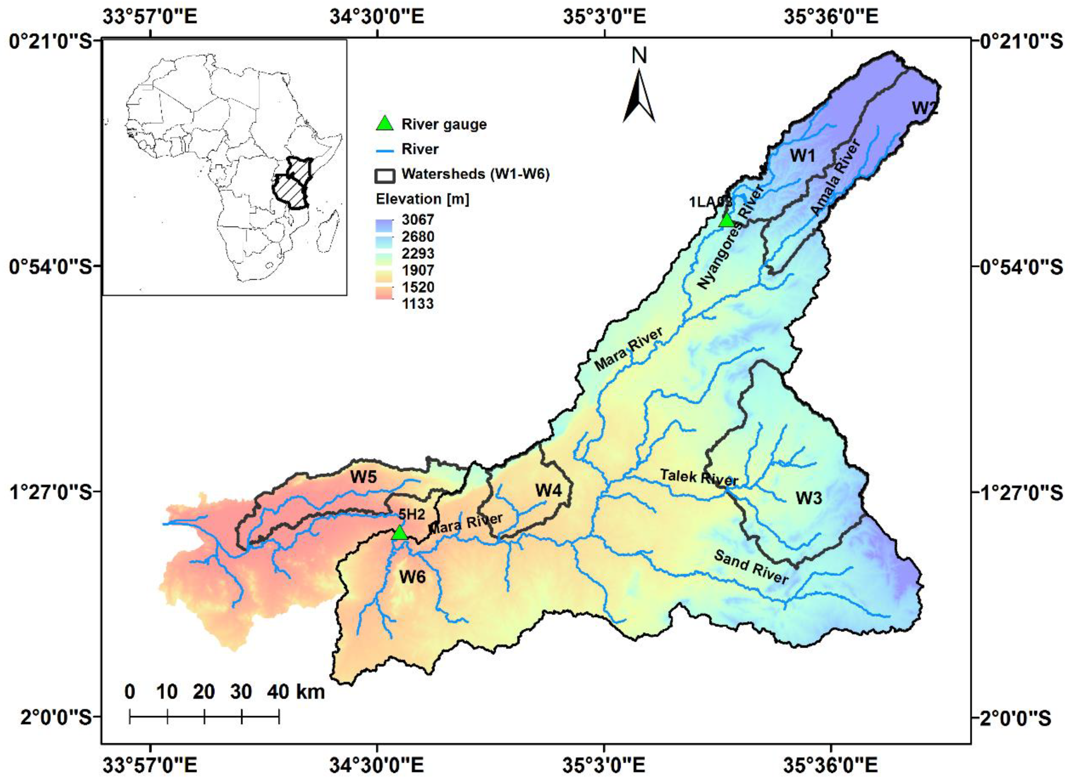
The Mara River originates from the forested Mau Escarpment (about 3000 m.a.s.l.) and drains 13,750 km2, of which approximately 65% is located in Kenya and 35% in Tanzania (Figure 2). The Amala and Nyangores Rivers are the only perennial tributaries draining the headwater region. The Talek and the Sand Rivers are the two most notable seasonal rivers stemming from Loita Hills in the southeast of the basin. The spatial rainfall distribution in the basin varies considerably (Table 1), with the highest and lowest mean annual rainfall being 1750 mm/year (Mau region) and 600 mm/year (southeast part), respectively [40]. The main factors influencing the rainfall distribution in the basin are its equatorial location and the range of landforms in the region, including high mountains, expansive plains and a large inland lake. Most parts of the basin receive rainfall with a bimodal pattern—the short rainy season (October–December) and the long rainy season (March–May). The rainfall in the short rainy season is driven by convergence and southward migration of the Intertropical Convergence Zone (ITCZ), whereas south-easterly trade winds drive the long rainy season. The mean annual temperature is approximately 25.5 °C and generally increases southwards.
The basin is endowed with significant biodiversity through a sequence of zones from a moist montane forest on the escarpment through a dry upland forest to scattered woodland and then the extensive grasslands of the savanna, with areas of scrub and thorn trees. The Serengeti–Masai Mara Plain is internationally famous for having the highest density and most diverse combination of large herbivores on earth [41].
The geology of the Mara Basin is composed mainly of volcanic rocks of the Tertiary and Nyanzian ages [40]. Dark volcanic origin soils are common on the escarpment and rangelands. Lower down, freely draining shallow soils are found. Poorly drained soils cover the plateau and support extensive grasslands or sorghum plantations. Finally, clay soils have accumulated in the river valleys and low-lying wetlands.

4. Methods and Data

4.1. SWAT Model Description

SWAT [35,42] is a comprehensive process-oriented and physically based simulator designed for use at a river basin scale. SWAT requires specific information about weather, soil properties, topography, vegetation and land management practices to simulate physical processes in a watershed. The water balance is the driving force underpinning all the processes in a basin [42]. The water balance equation (Equation (1); [42]) is solved at the hydrological response unit (HRU) level for the soil water content of the actual day (SWt) based on the initial soil water content of the previous day (SW0) and precipitation (P) as input water and losses via surface runoff (Qsruf), evapotranspiration (ET), groundwater flow (Qgw) and the amount of water leaving the soil profile to the vadose zone.
S W t = S W 0 + P Q s r u f E T W s e e p Q g w
In SWAT, a basin is partitioned into sub-basins, using topographic information. The sub-basins, in turn, are subdivided into HRUs that represent a unique combination of land use, soil type and slope class. All the hydrologic processes are simulated at the HRU level on a daily or sub-daily time step. The surface runoff is then aggregated to the sub-basin level for routing into a river network [42].
Vegetation plays a central role in basin hydrology and influences evapotranspiration, the largest water balance component in most climatic regions [1]. This study used SWAT-T [43], a modified SWAT model with improved vegetation growth dynamics for tropical conditions. The SWAT-T simulated leaf area index showed good agreement with the remote sensing-based estimates for the study area [43].

4.2. The Baseline Model

The Mara River Basin was set up using a high-resolution 30 m digital elevation model (DEM) (URL: http://earthexplorer.usgs.gov, accessed on 9 September 2015), land cover classes from the Africover project (URL: http://www.africover.org, accessed on 10 September 2015) and soil type classes from the World Harmonized Soil database [44] in ArcSWAT2012. The basin was subdivided into 89 sub-basins to spatially differentiate areas dominated by different land uses and/or soils with dissimilar impacts on hydrology. Each sub-basin was further discretized into about 1500 HRUs. The constructed model represents the 2002–2009 conditions. The SWAT model was forced by bias-corrected satellite rainfall from Roy et al. [45]. Weather data relevant to the reference evapotranspiration computation were obtained from the Global Land Data Assimilation System (GLDAS) [46]. Details regarding the model setup and forcing datasets can be found in Alemayehu et al. [43]. Table 2 presents the selected SWAT parameters based on previous studies [43,47,48,49,50] and expert knowledge for calibrating the baseline model. The baseline model has an improved model structure to simulate the vegetation growth cycle for the tropical region [43].

4.3. Calibration and Evaluation Framework

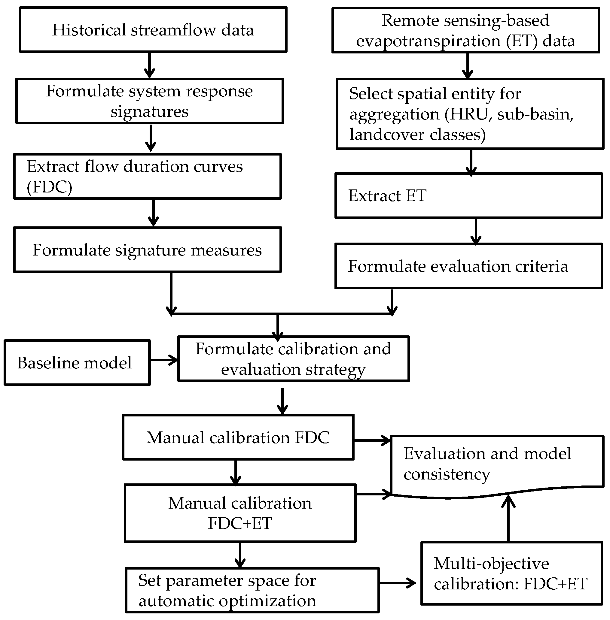
Figure 3 illustrates the general workflow for the calibration and evaluation procedure. The following section presents details about the information and data retrieval for manual and automatic calibration within a multi-objective framework.

4.3.1. The Procedures for the Extraction of Streamflow Signatures

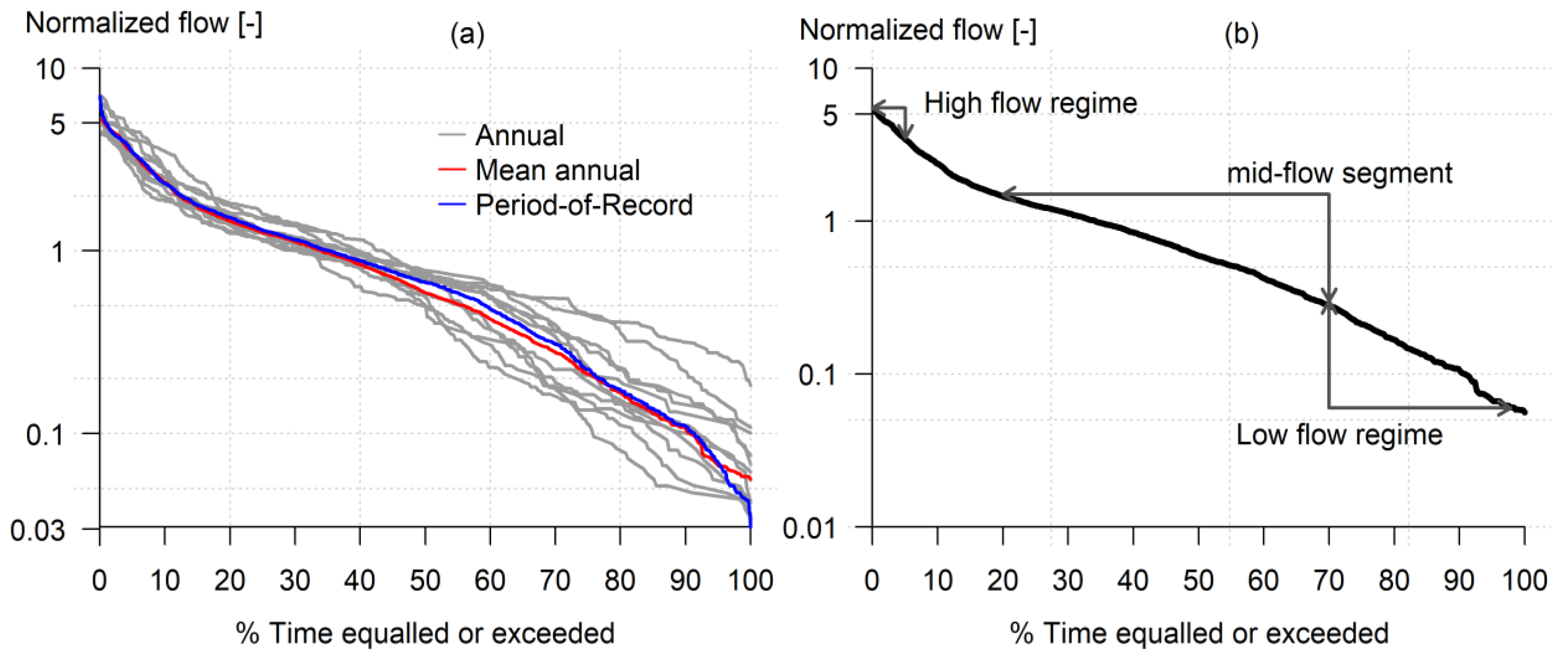
As illustrated in Figure 1, the availability of historical observed daily streamflow time series is relatively better for 1970–1990, which embodies valuable information about the dominant rainfall–runoff processes for the two watersheds (W1 and W6) (see location in Figure 2). FDCs extracted from such data can help make meaningful inferences about the watershed’s characteristics and streamflow behavior outside the observation window. Figure 4a depicts the annual FDCs derived using normalized daily streamflow for the Nyangores River (i.e., divided by the annual mean streamflow). As shown in Figure 4a and noted in Vogel and Fennessey [23], the mean annual FDC is not affected by the observation of abnormally wet or dry periods during the period of record. The procedures used to derive the streamflow signature information are outlined below:
  • After removing outliers, we considered years with 90% or more completeness assuming these adequately represent the annual streamflow regime.
  • Streamflow and thereby the associated FDCs are highly variable from year to year depending on the climate variability. We normalized the daily streamflow by dividing it by the mean and/or median streamflow. The normalization helps to amplify differences in FDCs due to aridity, geology and other factors.
  • We computed the dimensionless mean annual FDC using the normalized daily streamflow from step ii. Such curves represent the exceedance probability of streamflow in a typical year [22,23].
Figure 4b illustrates the three segments of the mean annual FDC (i.e., based on the normalized streamflow). We subjectively defined these segments such that the extracted signature information characterizes the streamflow regime pattern reasonably. In the remaining sections of this paper, the normalized mean annual FDC is referred to as the FDC unless otherwise stated.

4.3.2. Remote Sensing-Based Evapotranspiration

Remote sensing provides consistent estimates of evapotranspiration at various spatial (gridded) and temporal resolutions [27]. Alemayehu et al. [51] estimated the evapotranspiration of the study area using the Moderate Resolution Imaging Spectroradiometer (MODIS) land surface temperature based on the Operational Simplified Surface Energy Balance (SSEBop) [52] algorithm at a 1 km spatial scale and an 8-day temporal resolution (2002–2009). The authors reported that monthly evapotranspiration estimates exhibit good linear associations (i.e., r = 0.80) with the globally upscaled eddy covariance measurement-based ET product [53]. Additionally, this evapotranspiration product explained about 52% of the observed variability in the 16-day normalized difference vegetation index (NDVI) [53]. We used these evapotranspiration data to constrain the SWAT model. Since the SWAT model HRUs are non-georeferenced areas within a sub-basin, the remote sensing-based evapotranspiration was extracted per SWAT land cover class. Here, we used only the dominant land cover classes to reduce the uncertainty from the remote sensing estimates due to the land cover mix in the 1 km pixels. In this study, 8-day remote sensing-based evapotranspiration for evergreen forest, savanna grassland and shrubland was used to constrain the SWAT simulated evapotranspiration at the HRU level aggregated per land cover class.

4.3.3. The Stepwise Spatial Calibration Strategy

Our calibration framework was designed to maximize the effective use of the available spatial information to constrain the model parameters. Our study area involves two watershed categories—the humid watersheds in the headwater region (i.e., sub-basins 1–18) and the semi-arid watersheds (i.e., sub-basins 19–89). The SWAT parameters (Table 2) for the headwater region were adjusted first, and upon achieving a convincing model structure, the parameters for the remainder of the basin were then adjusted. We used relative change and replacement approaches to adjust the SWAT parameters as shown in Table 2. The former adjustment accounts for spatial variability in the parameters, while the latter assigns a space-invariant parameter value. The following section presents the details of the manual and automatic calibration procedures.

4.3.4. The Manual Calibration Strategy

An initial model calibration was conducted with a manual adjustment of parameters based on expert knowledge. Although subjective, in data-scarce basins, the adjustments of model parameters can indeed be based on an understanding of the dominant hydrological processes. Hrachowitz et al. [16] demonstrated the potential of an expert-knowledge-driven strategy for constraining hydrologic models.
For the manual calibration, we used two steps: (i) constraining the model parameters using only streamflow signatures; (ii) further constraining the SWAT parameters that control the evapotranspiration processes using remote sensing-based evapotranspiration data. These two experiments aim to investigate the synergy of using streamflow signature indices and remote sensing-based evapotranspiration for model evaluation in data-scarce basins.
The use of several diagnostic streamflow signatures during the manual calibration can help constrain different aspects of the simulated streamflow simultaneously. The high-streamflow regime signature (exceedance probability < 0.05) is useful to constrain parameters that control the surface runoff generation (Figure 4). The slope of the mid-flow segment of the FDC (exceedance probability between 0.2 and 0.7) provides information to constrain parameters relevant to infiltration and the redistribution of water in the soil profile. The low-streamflow regime signature (exceedance probability between 0.7 and 1.0) is helpful for adjusting the baseflow response. The parameters that control evapotranspiration processes were constrained using the remote sensing-based evapotranspiration product [51].

4.3.5. The Automatic, Multi-Objective Calibration Strategy

Despite the advantage of expert knowledge to manually adjust model parameters and thus improve the “realism” of the representation of the dominant hydrologic processes, it is cumbersome to objectively explore and illustrate the trade-offs within the feasible parameter space. We therefore used the manual calibration procedure to better pose the inverse problem for applying an efficient automated multi-objective optimization. The initial parameter range was set based on our observation during the manual calibration (Table 2). To explicitly solve the multi-objective, multi-modal problem, we used a global optimization approach to iteratively converge towards a discrete approximation of the Pareto set solutions. The multi-objective problem with M objectives is defined as
min ( w . r . t .   x   F ( x ) = ( F 1 ( x ) , F 2 ( x ) , F 3 ( x ) , , F M ( x ) ) ,   x ϵ Ω
where F(x) = F1(x), F2(x), …, FM(x) represents a set of M objectives (criteria), whereby each criterion measures model performance in a different aspect, and x is the model parameter. In such a formulation, the solution consists of non-dominated Pareto set solutions in the feasible parameter space (Ω) corresponding to various trade-offs among the objectives. Therefore, a model simulation using every member of the Pareto set will reproduce part of the streamflow signatures and/or evapotranspiration per land cover class better than every other member of the Pareto set, but the trade-off will be that some other characteristics of the streamflow signatures and/or evapotranspiration will not be as well matched. The predictive uncertainty of the calibrated SWAT model for simulating streamflow and evapotranspiration was measured based on the range of simulations using the parameter value range in the Pareto optimal solutions. For this, we used the recently developed Borg multi-objective evolutionary algorithm (Borg MOEA) [54,55], as implemented in the R programming environment by Hadka et al. [56]. We ran the algorithm for 3000 function evaluations, using the five objective functions described in the next section.

4.3.6. The Evaluation Criteria

The Statistical Measures

The model calibration was conducted from 2002 to 2007 for both streamflow and evapotranspiration, and the calibrated model was further verified for the period 2008–2009. We used three statistical measures (evaluation criteria) to assess the degree of “closeness” between the simulated and observed hydrologic variables. Yilmaz et al. [13] demonstrated that biases in the high streamflow volume (BFHV), the mid-segment slope of the FDC (BFMS) and the low streamflow volume (BFLV) are useful diagnostic measures to constrain a hydrologic model. Therefore, we used these measures to quantify the degree of agreement between the SWAT simulated streamflow (QS) signatures and the observed historical streamflow (QO) signatures. The measures are formulated as follows [13]:
B F H V = h = 1 H ( Q S h Q O h ) h = 1 H Q O h
where h = 1, 2, …, H are the indices for the normalized streamflow magnitudes with exceedance probabilities lower than 0.05.
B F M S = | l o g ( Q S m 1 ) l o g ( Q S m 2 ) | | l o g ( Q O m 1 ) l o g ( Q O m 2 ) | | l o g ( Q O m 1 ) | | l o g ( Q O m 2 ) | × 100
where m1 and m2 are the lowest and highest normalized streamflow exceedance probabilities (0.2 and 0.7, respectively) within the mid-segment of the mean annual FDC.
B F L V = l = 1 L [ l o g ( Q S l ) l o g ( Q O l ) ] l = 1 L [ l o g ( Q O l ) l o g ( Q O 0.98 ) ] × 100
where l = 1, 2, …, L are the indices for the normalized streamflow magnitudes within the low-streamflow regime of the FDC (0.7–1.0 exceedance probabilities).
The simulated and remote sensing-based evapotranspiration agreements were measured using the Pearson correlation coefficient (r) and the percent of bias (pbias). We used r as an evaluation criterion because the SWAT simulated and remote sensing-based evapotranspiration do not have the same definition and hence the same values; however, they should be strongly correlated [33]. The additional use of pbias is considered important here, as r does not account for possible biases.
Additionally, recently, the Mau Mara Serengeti (MaMaSe) Sustainable Water Initiative (http://mamase.org/, accessed on 1 September 2015) has made an effort to create a knowledge base on the hydrology of the Mara Basin (in Kenya) at ILA03. This initiative has made quasi-observed daily streamflow for 2002–2007 available. Therefore, data were used to evaluate the calibrated SWAT model based on the normalized mean squared error (NMSE), the index of agreement (d), r and pbias.

Diagnostic Consistency Assessment

Apart from statistical performance measures, it is important to test the extent to which a model is consistent with our understanding of reality [9,16,57], a critical step in poorly gauged basin hydrologic model calibration.
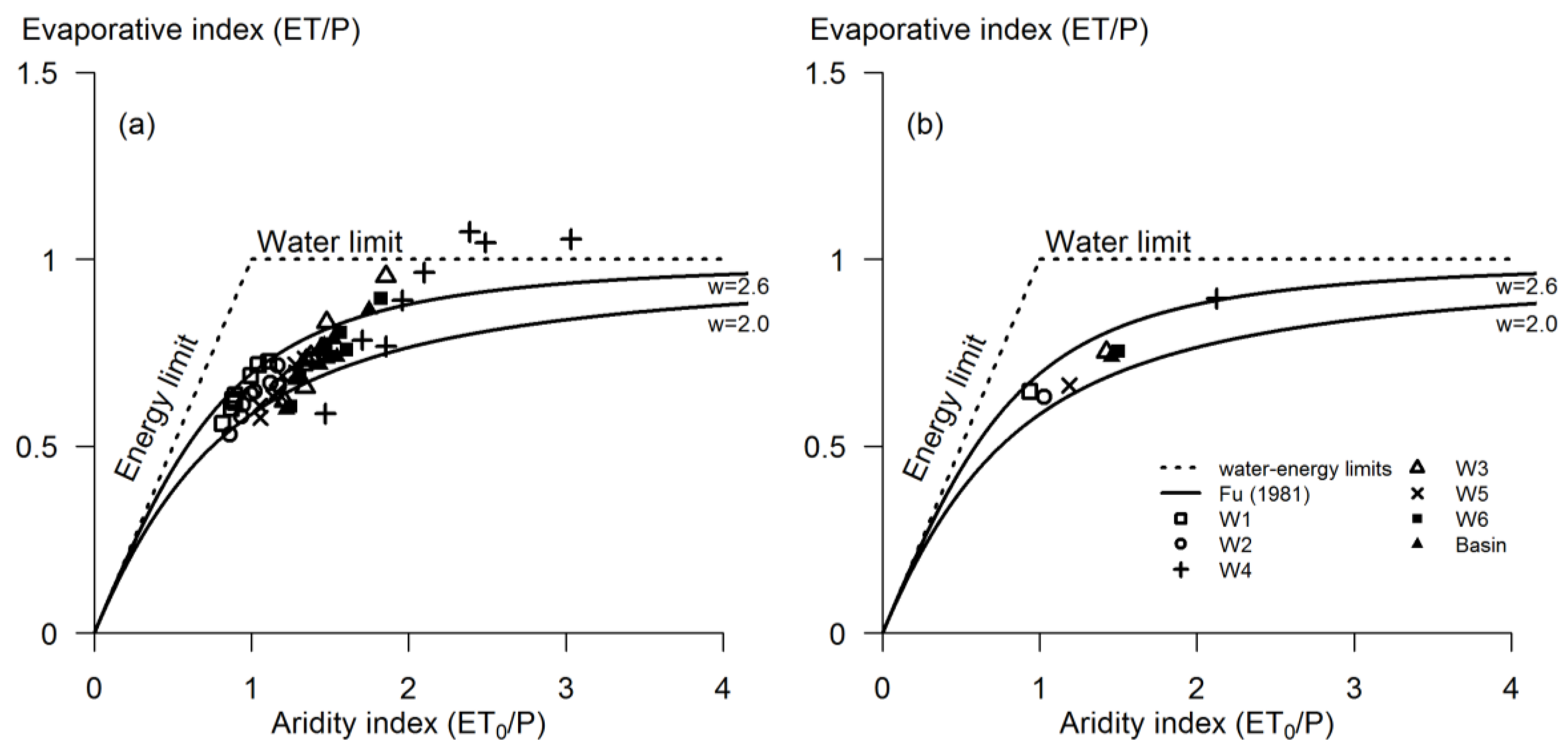
Budyko [58] postulated that the available energy and water primarily control the long-term catchment water balance, whereas the characteristics of the catchment (soil, topography, geology, land cover, etc.) play a secondary role [59,60,61]. We used the Budyko diagram—which depicts the evaporative index (ET/P) as a function of the aridity index (ET0/P)—for a qualitative diagnostic assessment of the dominant hydrologic processes as simulated by the calibrated SWAT model. Additionally, to evaluate the consistency of the simulated annual evapotranspiration and total water yield across the basin, we fitted the Budyko-like Fu curve [62]. In Fu’s equation (Equation (6)), the parameter w represents the integrated effects of landscape characteristics on the water balance dynamics of a watershed [61].
E T P = 1 + E T 0 P [ 1 + ( E T 0 P ) w ] 1 / w
For this purpose, we identified six watersheds across the study area with varying physiographic characteristics and climates (see Figure 2 and Table 1). We assumed that the water balance simulations from a calibrated model should exhibit a consistent pattern with the Budyko diagram across several watersheds within the basin.

4.3.7. Relative Performance Comparison

To evaluate the added value of each calibration strategy, we compared the relative performances of the calibrated SWAT models to the baseline model performances. Here, the relative performance (RP) for streamflow signatures (BFHV, BFMS and BFLV) and evapotranspiration (pbias) of the baseline and calibrated SWAT models was computed as
R P = ( | B i a s B a s e l i n e | | B i a s C a l i b r a t e d | ) | B i a s B a s e l i n e | × 100
where BiasBaseline is the performance of the baseline model, and BiasCalibrated is the performance of the calibrated model. Meanwhile, the relative performance of the correlation in the 8-day ET was computed as
R P = ( | C o r r e l a t i o n B a s e l i n e | | C o r r e l a t i o n C a l i b r a t e d | ) | C o r r e l a t i o n B a s e l i n e | × 100
where CorrelationBaseline is the performance of the baseline model, and CorrelationCalibrated is the performance of the calibrated model. RP values greater than 0 indicate improvement in model performance, a reduced bias and an increased correlation. On the other hand, RP values less than 0 indicate a deterioration in model performance.

5. Results

5.1. The Baseline Model Performance

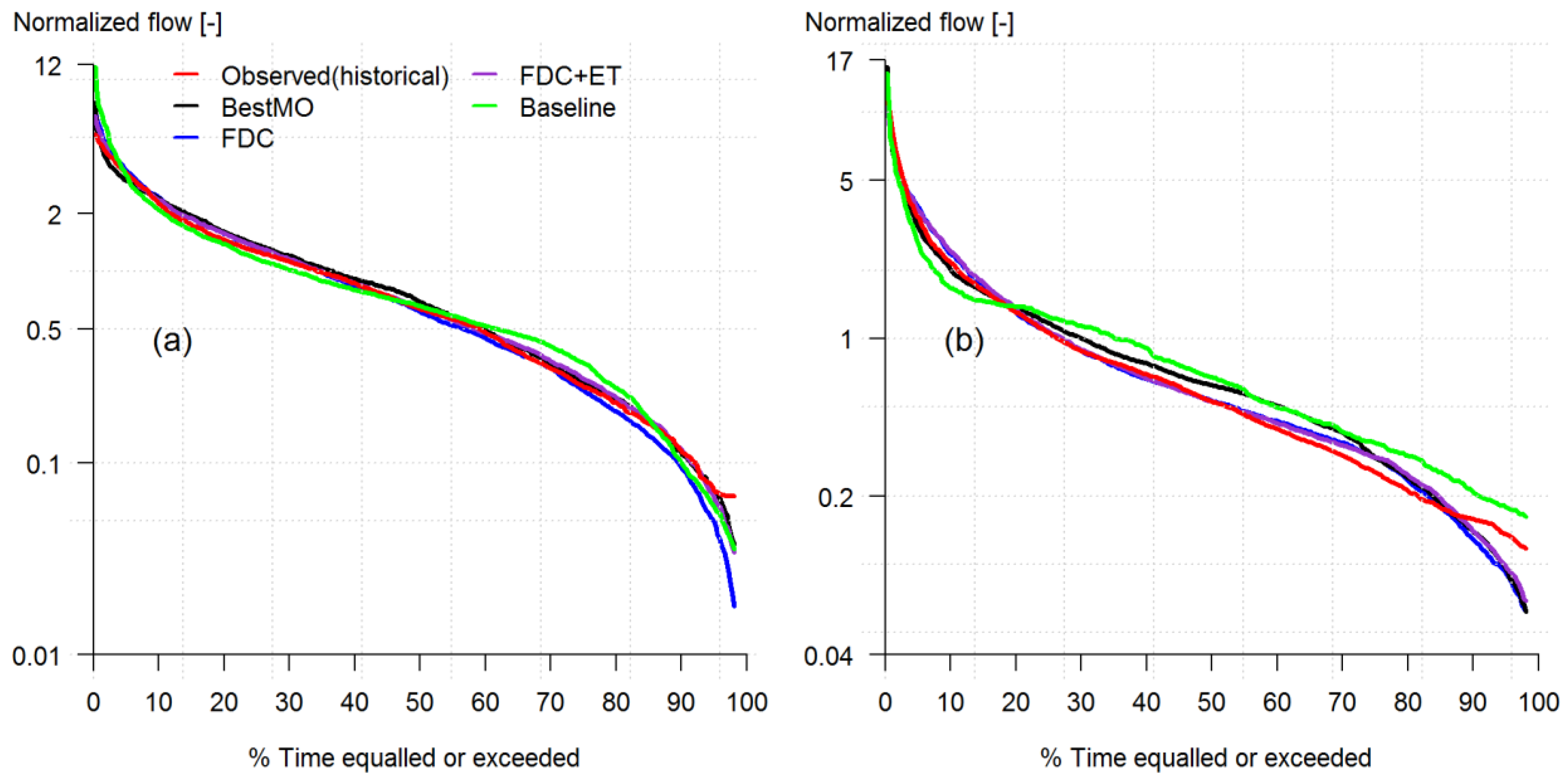
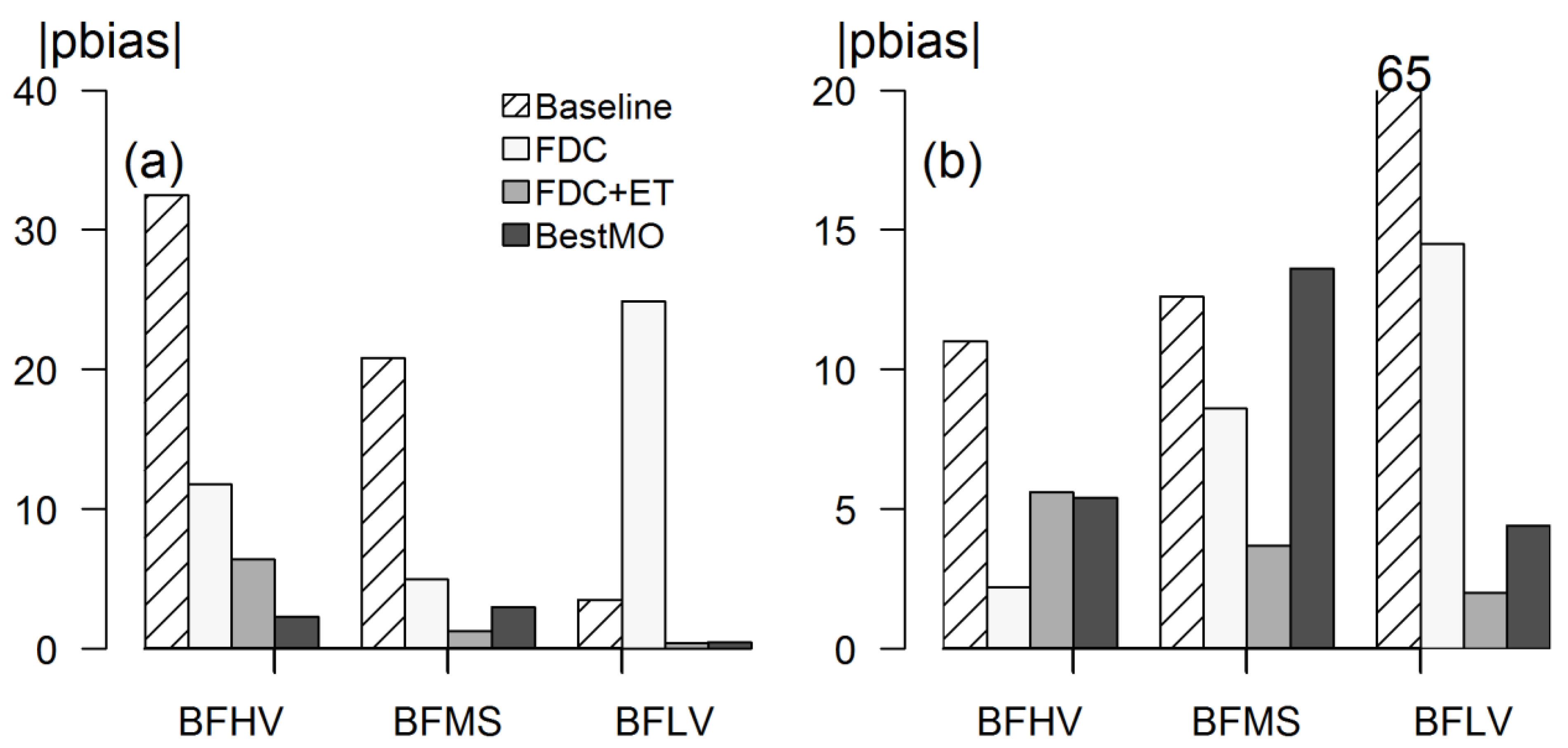
The FDCs derived from historical observations and simulations from the uncalibrated baseline model show a similar pattern for the Nyangores River (Figure 5a). Despite the matching streamflow regime patterns, there is a substantial bias in the simulated FDC high- and low-streamflow regimes (Figure 6a). The bias in the high-streamflow regime is about 32% for the gauge located in the headwater region, suggesting a high-streamflow regime overestimation by the baseline model. On the other hand, the bias in the slope of the FDC is about −21%, which indicates underestimation in the slope of the FDC compared to the historical observed FDC. A gentler slope in an FDC, in general, suggests a slower response of a basin to precipitation forcing [13]. We note the good performance of the baseline model in simulating the low-streamflow regime, with a bias of 3.5%.
The performance of the baseline model for the Mara River is illustrated in Figure 5b and Figure 6b. The biases in the high-streamflow regime and the slope of the FDC are about −11% and −12.6%, respectively. Hence, the baseline model underestimates the high-streamflow regime and leads to a higher infiltration and high contribution of groundwater to streamflow, as indicated by the flatter slope in the FDC compared to the observed historical streamflow signatures. In contrast, the bias in the low-streamflow regime is about 65%, which means the baseline model overestimates the low-streamflow regime compared to the historical observed streamflow, as shown in Figure 5b.
We compared the 8-day SWAT simulated HRU level evapotranspiration aggregated per land cover class with the remote sensing-based estimates from 2002 to 2007 (Figure 7). The median correlations between the baseline model simulated and remote sensing-based evapotranspiration are about 0.65 and 0.61 for the savanna grassland and shrubland land cover classes, respectively. We also noted a low median correlation (i.e., r = 0.48) for the evergreen forest cover type. Although the baseline model simulated evapotranspiration corresponds somewhat to the remote sensing-based estimates for the three land cover classes, there is an overestimation bias of up to 12%.

5.2. The Manual Calibration Results

The manual calibration of the SWAT model was performed stepwise to reduce biases in streamflow. First, we calibrated the model using only the FDC signature measures for sub-basins 1–18. Subsequently, the parameters for the dominant part of the basin (sub-basins 19–89) were adjusted using the FDC signature measures. As shown in Figure 6, constraining the SWAT model using the FDC signature measures reduced most of the biases observed from the baseline model. However, the calibrated model shows a poor performance in simulating the low-streamflow regime for the Nyangors River, with a bias of about 25%, but this bias was reduced substantially from 65% to −15% for the Mara River. The poor performance in the low-streamflow regime is partly attributed to the parameters that control recharge and evapotranspiration. At this point, the parameters that control the evapotranspiration simulation (such as SOL_AWC, ESCO and SOL_Z) in the “calibrated model” are the same as in the baseline model, and thus the simulated 8-day evapotranspiration shows slightly better and/or similar performances when compared with the remote sensing-based estimates (Figure 7). As shown in Figure 7a, the model calibrated using streamflow signatures only shows reduced biases for savanna grassland (up to 50%) and shrubland evapotranspiration, with a slight deterioration in their correlations. On the other hand, we noted an increase in the bias for evergreen forest evapotranspiration, while the correlation improved considerably.
Figure 6 and Figure 7 show that the SWAT model reasonably reproduces the observed streamflow regime signatures (i.e., with low biases) when the remote sensing-based evapotranspiration and streamflow signatures constrain the model. The addition of evapotranspiration in the SWAT model calibration reduced the biases in the streamflow signature measures to lower than 6.5% and 5.6% for the Nyangores and Mara Rivers, respectively. Interestingly, the use of remote sensing-based evapotranspiration effectively helped in constraining the parameters that control the redistribution of soil moisture and recharge, resulting in lower biases in the low-streamflow regime and the slope of the FDC than when the model was constrained using only the streamflow signatures. Additionally, the simulated evapotranspiration reveals relatively low biases (pbias < 4.8%) and better correlations (r > 0.66) for the three dominant land cover classes (Figure 7b).

5.3. The Automatic, Multi-Objective Calibration Results

Next, we calibrated the SWAT model parameters using a multi-objective optimization framework to explore trade-offs between the streamflow signatures and remote sensing-based evapotranspiration. In principle, this should help expose deficiencies in the model structure [20,63] and illustrate the interaction between parameters.
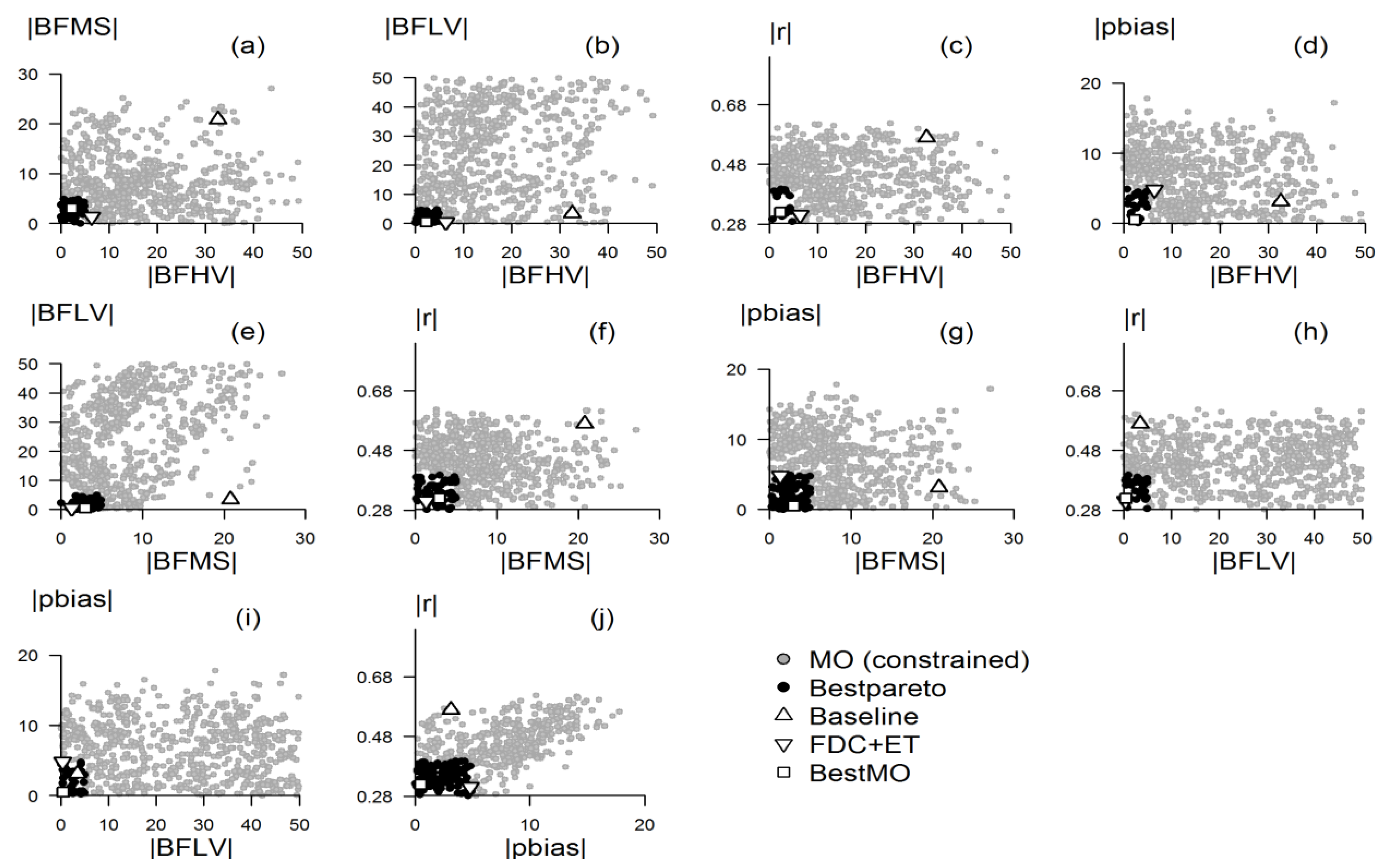
Figure 8 presents the parallel coordinates plot to visually represent the five-dimensional evaluation criteria, where each line represents a trade-off in the multi-criteria evaluation. Here, the “parallel plots” clearly indicate that the “model calibration problem is inherently multi-objective” [63]. Additionally, Figure 9 presents the trade-offs considering a combination of two criterion spaces (i.e., 5 ×2 = 10 combinations). The gray lines (dots) in Figure 8 and Figure 9 represent the subset of evaluation measures (out of 3000 function evaluations) that satisfy the within 50% bias for the streamflow signatures and evapotranspiration, as well as a higher than 0.3 correlation for evapotranspiration (i.e., MO (constrained)). What is apparent from these multiple illustrations is the existence of a high degree of compensation within the five evaluation measures, suggesting that a parameter set that returns a low bias for the high-streamflow regime results in a poor performance for the other evaluation criteria and vice versa. This is particularly notable for watersheds dominated by a semi-arid climate (i.e., sub-basins 19–89) compared to the semi-humid watersheds (i.e., sub-basins 1–18) (see Figures S1 and S2). Interestingly, however, there is less compromise between the biases in the slope of the FDC and the goodness-of-fit measures for evapotranspiration (i.e., r and pbias), thereby resulting in considerable parameter solution sets that satisfy a less than 5% bias and a correlation above 0.6 (black dots in Figure 9f,g and Figure S2f,g). For instance, for sub-basins 19–89, there are about 487 (r vs. BFMS) and 218 (pbias vs. BFMS) parameter solution sets out of 685 solutions (MO (constrained)). This signifies that a good estimation of model parameters that control the vertical soil water redistribution such as SOL_AWC and ESCO using signature measures from the slope of the FDC could also assure a good evapotranspiration prediction and vice versa.
Solutions along the Pareto front (i.e., the lower part of the “parallel plot” and the diagonal in the two-dimensional space) are “equally optimal”, in the sense that a user can choose one particular solution based on the importance of the calibration criteria and/or the intended application of the model. In this study, we set a threshold for the bias and the correlation indices such that only Pareto set solutions with relatively better (compromise) criterion values are selected to simulate the water balance components. The threshold for the bias was set to lower than 10% and 15% for sub-basins 1–18 and sub-basins 19–89, respectively, for the three streamflow signature measures, whereas greater than 0.65 and less than 10% thresholds for the correlation and bias in evapotranspiration, respectively, were set for all three land cover classes. In doing so, a total of 13 (out of 781) and 11 (out of 685) Pareto set solutions (Bestpareto) were selected for sub-basins 1–18 and sub-basins 19–89, respectively. Finally, we chose one “best” multi-objective solution (BestMO) out of the selected Pareto set solutions, albeit involving some degree of subjectivity. The sampled parameter sets gave, on average, an acceptable performance across the five measures. However, the selected parameter values show a large spread, indicating a parameter identification problem. This can be partly attributed to the limited number of function evaluations (i.e., 3000) compared to the number of evaluation criteria involved in the multi-objective optimization. However, we believe this is sufficient to demonstrate the framework to calibrate watershed models using historical streamflow signature measures and remote sensing-based evapotranspiration in a multi-objective approach in data-limited basins.
As shown in Figure 5a and Figure 6a, the selected relatively best trade-off parameter set (BestMO) reproduces the observed streamflow signatures for both the Nyangores and Mara Rivers. For the Nyangores River, the biases of the three signature measures are lower than 4%. For the Mara River, the model shows good performances for both the high- and low-streamflow regimes, albeit a negative 14% bias (i.e., underestimation) in the slope of the FDC. As shown in Figure 7b, the selected Pareto set solutions also improve the correlations between the SWAT simulated and remote sensing-based evapotranspiration, with median correlations of 0.71 (evergreen forest), 0.69 (savanna grassland) and 0.65 (shrubland) at the 8-day scale. Additionally, the median biases are lower than 6% (Figure 7a).
Even though the simulated evapotranspiration for savanna grassland is improved when using the Pareto set solutions, the estimated evapotranspiration shows a positive bias (about 6%). This is linked to the negative biases noted for the slope of the FDC for the Mara River. For all the selected Pareto set solutions, the SWAT model shows an average negative bias of 10% for the slope of the FDC for the Mara River, indicating the limitation of the model in simulating the soil moisture redistribution and hence the subsurface flow. The slope of the FDC is strongly associated with SWAT parameters that control the vertical soil water redistribution (such as SOL_AWC, SOL_K and ESCO; see definition in Table 2). An increase in water storage in the soil results in a gentle slope in the FDC and an increase in soil evaporation and transpiration.
Figure 10 presents the mean annual FDCs of the simulated streamflow using the selected Pareto set solutions for the Nyangores and Mara Rivers. These plots depict a somewhat comparable streamflow regime pattern for the selected Pareto set solutions (BestPareto) for both rivers, indicating the extent to which the historical streamflow signatures and remote sensing-based evapotranspiration constrained the SWAT model parameters. The median streamflow ranges from 5.2 to 8.1 m3/s for the Nyangores River at Bomet and from 38 to 42.3 m3/s for the Mara River at Mines.

5.4. The Validation of the Calibrated Models

Table 3 summarizes the performance indices of the calibrated SWAT models for simulating evapotranspiration during the validation period. We note the general positive biases of 12.1% (evergreen forest), 16.9% (savanna grassland) and 7.2% (shrubland) of the SWAT simulated evapotranspiration compared to the remote sensing-based estimates, regardless of the existence of fair correlations at the 8-day scale. The difference in the mean annual rainfall between the calibration and validation periods is minimal (5 mm), and hence rainfall could not justify the bias in the simulated evapotranspiration. Nevertheless, the reference evapotranspiration increases slightly by 63 mm in the validation period and thus leads to an increase in the SWAT simulated evapotranspiration. The other contributing factor is the consistent poor performance of the SWAT model during the calibration period in sub-basins 19–89, as depicted Figure 6b, where there is a bias of −13.6% in the slope of the FDC (BestMO). A negative bias in the slope of the FDC indicates soil water storage in the soil profile and hence leads to a flatter slope. The water stored in the soil profile subsequently increased the soil evaporation and transpiration. The biases in the satellite-based rainfall and evapotranspiration could also contribute to the observed poor performance in the SWAT simulated evapotranspiration.
Table 4 presents the summary statistics for the simulated streamflow for the evaluation period. On average, the calibrated models show a reasonable skill in reproducing the observed streamflow statistics. The simulated median streamflow using the manually calibrated SWAT model for the Nyangores River during the validation period shows a good match with the long-term historical median streamflow. However, the simulated streamflow for the Mara River is double the long-term median streamflow. It is acknowledged here that the lack of overlapping observations hampers rigorous validation of the model performance. Therefore, to further evaluate the skill of the calibrated model parameters, we compared the daily simulated streamflow with observations at the Nyangores watershed. Note that the quasi-observed streamflow time series were not used during the calibration period.
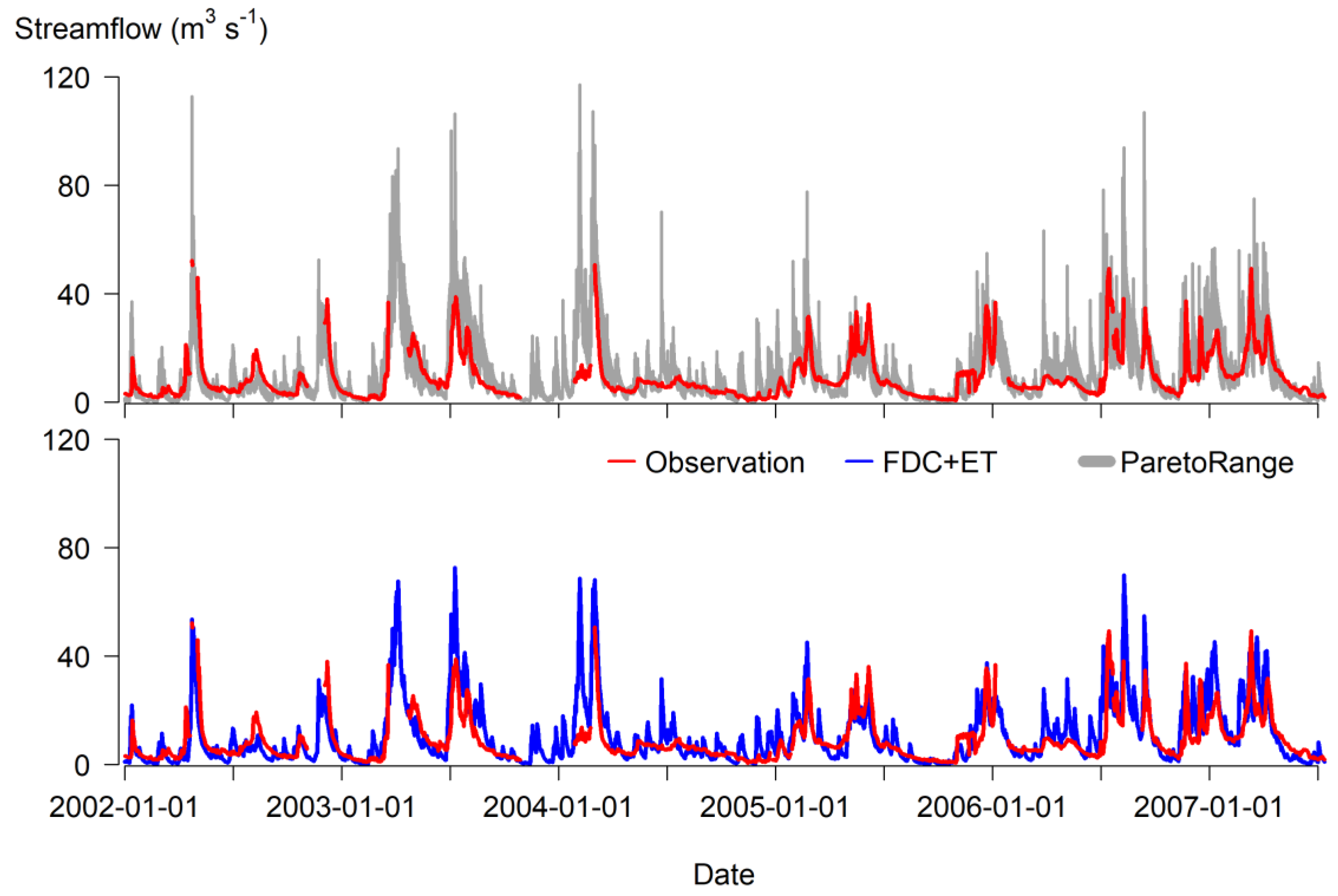
The simulated streamflow using the selected 13 Pareto set solutions compares fairly with the observed streamflow (2002–2007). The median values for the NRMSE, the IA, Pearson’s correlation r and the KGE are about 0.18, 0.77, 0.69 and 0.53, respectively, indicating the relatively good performance of the calibrated model in simulating daily streamflow (see Figure S3). Figure 11 compares the simulated daily streamflow with observations. Close visual inspection shows that the model tends to overestimate the peak streamflow; this is clearly shown by the large scatter in Figure 11 (top panel) using 13 Pareto set solutions (ParetoRange). In general, however, the calibrated SWAT model shows a better streamflow simulation ability than the baseline model.

5.5. Consistency Assessment

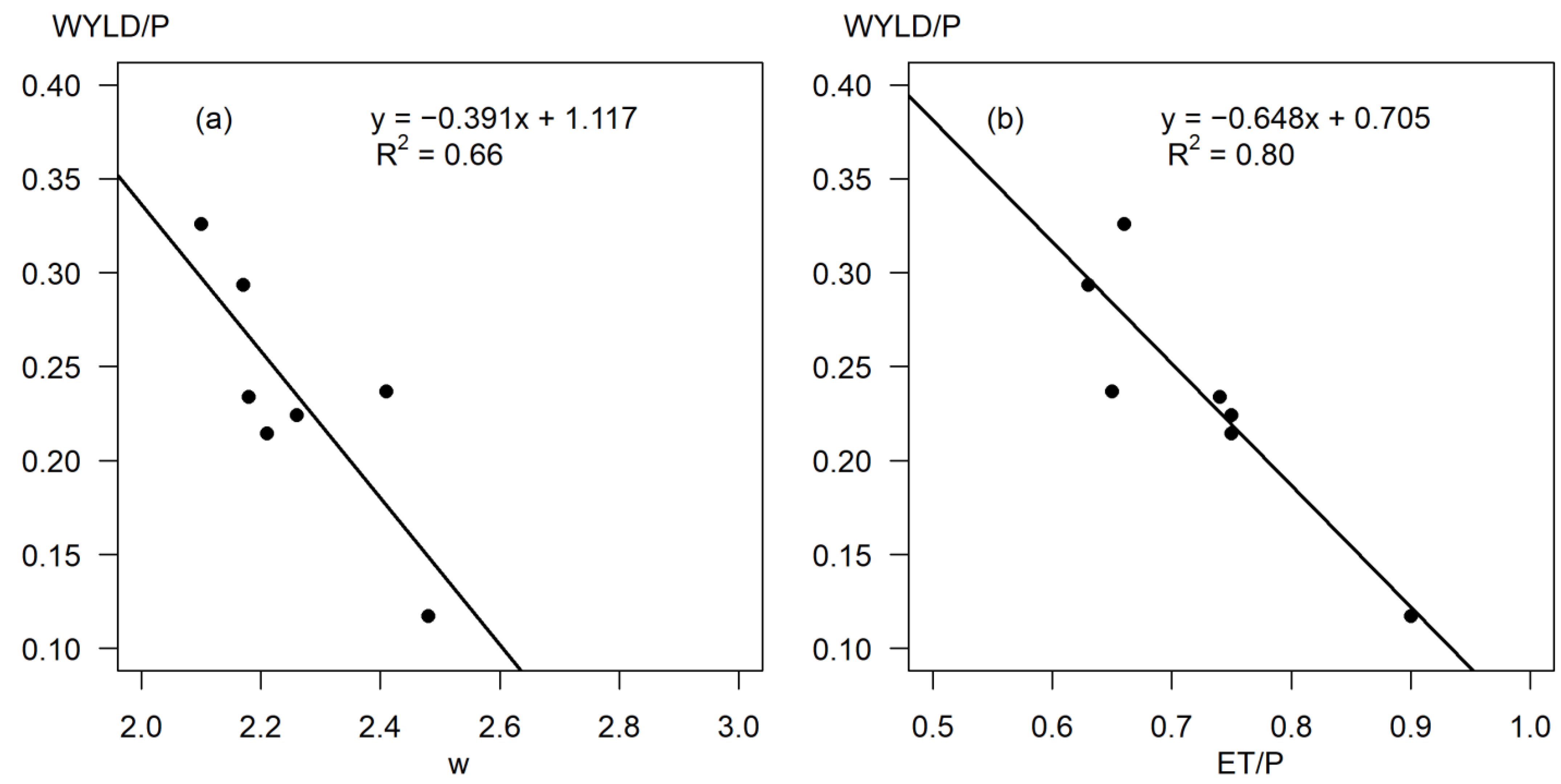
We reran the calibrated SWAT models for 2002–2009 to evaluate the simulations in the context of varying biotic and abiotic factors across the selected watersheds in the Mara Basin (Table 1). Figure 12 shows the Budyko diagrams for six watersheds (W1–W6) and the whole basin. Both the annual and mean annual evaporative index (ET/P) and the aridity index (ET0/P) are within the domain of the energy and water limit boundary, suggesting the consistency of the simulated water balance components. However, in the semi-arid watershed W4 (see location on Figure 2), the evaporative index slightly surpasses the water limit for the years 2005, 2007 and 2009 (Figure 12a), indicating the annual evapotranspiration exceeded the annual rainfall. Remarkably, 2005 and 2009 were drought years in that region [64,65], and hence the soil water evaporation and the root water uptake by the vegetation exceeded the rainfall. Figure 13a presents the correlation of the runoff coefficient—the ratio of total water yield and rainfall—with the fitted Fu w parameter values and the evaporative index, while Figure 13b depicts the runoff coefficient relationship with the evaporative index (ET/P) for watersheds W1–W6 and the whole basin. The high negative correlation (r = 0.81) between the runoff coefficient and w suggests that watersheds with a high annual evaporation rate tend to have a lower runoff coefficient (i.e., low water yield). This observation sufficiently reflects the watershed characteristics presented in Table 2, whereby in the semi-arid watersheds (e.g., W3 and W4), the dominant part of the annual rainfall leaves the watersheds as evapotranspiration. In summary, the calibrated SWAT model using streamflow signatures and evapotranspiration can consistently simulate the basin water balance components.

5.6. Relative Performance Comparison

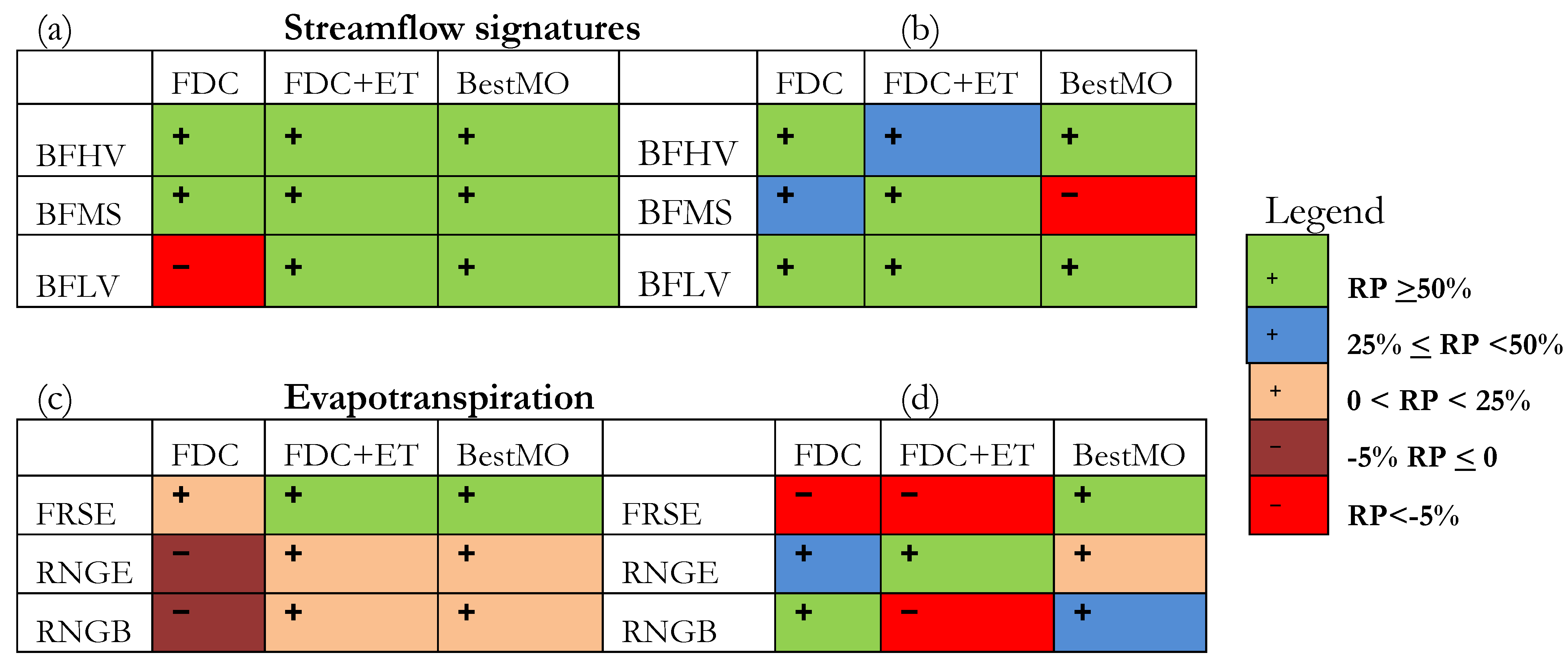
Figure 14 illustrates the relative performance of SWAT models calibrated using only streamflow signatures (FDC), using streamflow signatures and remote sensing-based evapotranspiration manually (FDC+ET) and automatically in a multi-objective framework (BestMO) compared to the baseline model performance. As shown in Figure 14a,b, we note the general above 50% relative performance of all the calibration approaches for streamflow signatures for the Nyangores and Mara Rivers, suggesting a substantial reduction in biases. However, the relative performance for the biases in the low-streamflow regime for the Nyangores River exhibits a decrease in model performance when calibrated using only the streamflow signatures (see Figure 6a). This indicates that the baseline model has a lower bias in simulating the baseflow regime for the Nyangores River. The relative performance of SWAT in simulating evapotranspiration for evergreen forest depicts a deterioration for the calibrated models using streamflow signatures alone (FDC) and when coupled with remote sensing-based evapotranspiration (FDC+ET). Yet, the calibration approaches overall improved the performances in correlation by up to 25% for all the land cover classes. The slight improvements in evapotranspiration after calibration are partly attributed to the calibrated vegetation growth parameters in the baseline model [43].
The calibration exercise revealed that the coupling of streamflow signatures with remote sensing-based evapotranspiration decreases the biases in the simulated streamflow signatures and increases the correlation of evapotranspiration (see Figure S4). We highlight the relatively better performance of the calibrated SWAT model using streamflow signatures and remote sensing-based evapotranspiration in sub-basins 1–18 than in sub-basins 19–89. This is in agreement with Kunnath-Poovakka et al. [34], who noted the better performance of calibration using remote sensing-based evapotranspiration in catchments with medium to high average runoff. Overall, we conclude that the simulated evapotranspiration is improved when the model is constrained by both the streamflow signatures and the remote sensing-based evapotranspiration.

6. Discussion

6.1. Parameter Estimation

One of the challenges in poorly gauged/ungauged basins is the parameter estimation of hydrologic models due to the lack of in situ observation to adjust model parameters. This study attempted to estimate selected SWAT model parameters using historical streamflow signatures and remote sensing-based evapotranspiration manually and automatically in a multi-objective framework. Table 5 presents the calibrated SWAT parameters for sub-basins 1–18 and sub-basins 19–89. For sub-basins 1–18, the manually calibrated CN2, which controls the runoff generation at the HRU level, was reduced substantially by 33%, suggesting a lower surface runoff generation potential and hence that more water will infiltrate into the subsurface. The surface runoff lag coefficient (SURLAG) was also reduced from 4 (initial value) to 0.1, meaning the generated runoff contributes to the main channel with less delay (lag). The soil water content (SOL_AWC) also decreased by about 21%, and therefore more soil water percolates to the shallow aquifer as recharge. This will result in a high groundwater contribution as baseflow and deep aquifer recharge. These are reflected by the baseflow recession constant (ALPHA_BF) of 0.9 and deep aquifer recharge (RCHRG_DP) of 0.7. The addition of the remote sensing-based evapotranspiration to constrain the SWAT parameters (FDC + ET) increased the soil depth by 60% and slightly increased the SOL_AWC (i.e., by 3%) compared to the parameter estimates using historical streamflow signatures alone. Compared to sub-basins 1–18, sub-basins 19–89 tend to generate more surface runoff with less groundwater contribution. Thus, CN2 increased by 14%, and ALPHA_BF was reduced to 0.02.
We noticed that the parameter range for the selected Pareto set solutions using the Borg MOEA [54] shows a wide range, but it is not sufficient to envelope the observed streamflow for the Nyangores River (Figure 11, top panel). The selected Pareto range captured about 50% of the observed streamflow, and this increases to about 80% if we consider a large sample from a Pareto set solution (i.e., 781 in MO (constrained) in Figure 8). This indicates that the failure of the selected Pareto range in capturing high and low streamflow in some instances is mainly attributed to the tunable model parameters given the limited number of function evaluations (i.e., 3000 simulations) during the optimization using five objective functions. Therefore, this requires future research with a more computational budget to properly assess the range of Pareto set solutions. Additionally, the satellite-based datasets that were used as model input (i.e., rainfall) and observed calibration data (i.e., evapotranspiration) could carry biases due to cloud contamination, particularly in the mountainous part of the basin, and thus could contribute to the limited performance of the selected Pareto set solutions.

6.2. Effects of Calibration on the Soil Water Redistribution

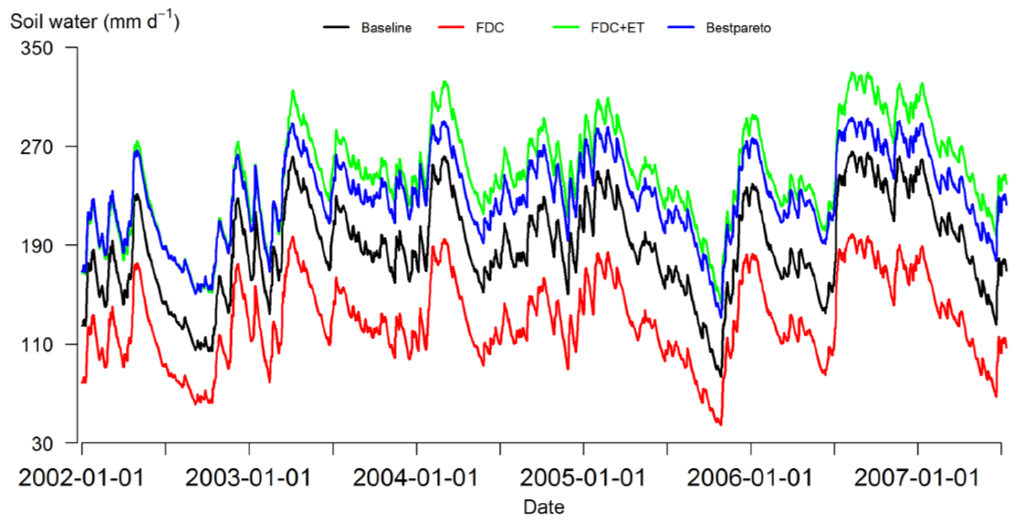
One of the major synergies noted in this study is the effectiveness of the streamflow signature measures and remote sensing-based evapotranspiration to constrain the SWAT model parameter related to the soil water balance. As illustrated in the automatic multi-objective calibration in Section 5.3, a low bias in the slope of the FDC tends to give a high correlation and low bias for evapotranspiration. Figure 15 presents the daily soil water content simulated by the baseline and the calibrated SWAT models averaged over the basin. The daily mean soil water content ranges from 129 mm/d (for calibration with streamflow signatures only) to 246 mm/d (for calibration with streamflow signatures and remote sensing-based evapotranspiration), suggesting considerable change due to the calibrated soil parameters. The soil water content is a function of rainfall, soil texture and land cover type, among other factors. As a result, we can observe the remarkable spatial variation differences when the SWAT model is calibrated with streamflow signature measures and remote sensing-based evapotranspiration, as shown in Figure 16. For instance, as depicted in Figure 16b for 5 May 2002 for the model calibrated using streamflow signatures and remote sensing-based evapotranspiration, the average HRU-level soil water content is about 266 mm/d (±102 mm/d), indicating substantial spatial variation in the soil water content. A noticeable difference, on average 98 mm/d (±49 mm/d), is marked between SWAT models calibrated with streamflow signature measures alone and streamflow signature measures combined with remote sensing-based evapotranspiration, as shown in Figure 16c. The observed substantial changes in the calibrated SWAT model simulated soil water content are mainly attributed to the changes in the soil depth (SOL_Z), the available soil water content (SOL_AWC) and ESCO, as presented in Table 5.

6.3. Can Streamflow Signatures and Remote Sensing-Based Evapotranspiration Constrain a Distributed Model Meaningfully?

In the preceding sections, we discussed how available information can be used innovatively to constrain the parameters of a semi-distributed hydrologic model in a data-scarce region. In a multi-objective framework, we explored different calibration strategies to constrain the SWAT model using both streamflow signatures and remote sensing-based evapotranspiration. The statistical evaluation metrics indicate that a relatively good result has been achieved, meaning that the calibrated SWAT model can reproduce the observed historical streamflow signatures and the overlapping remote sensing-based evapotranspiration estimates.
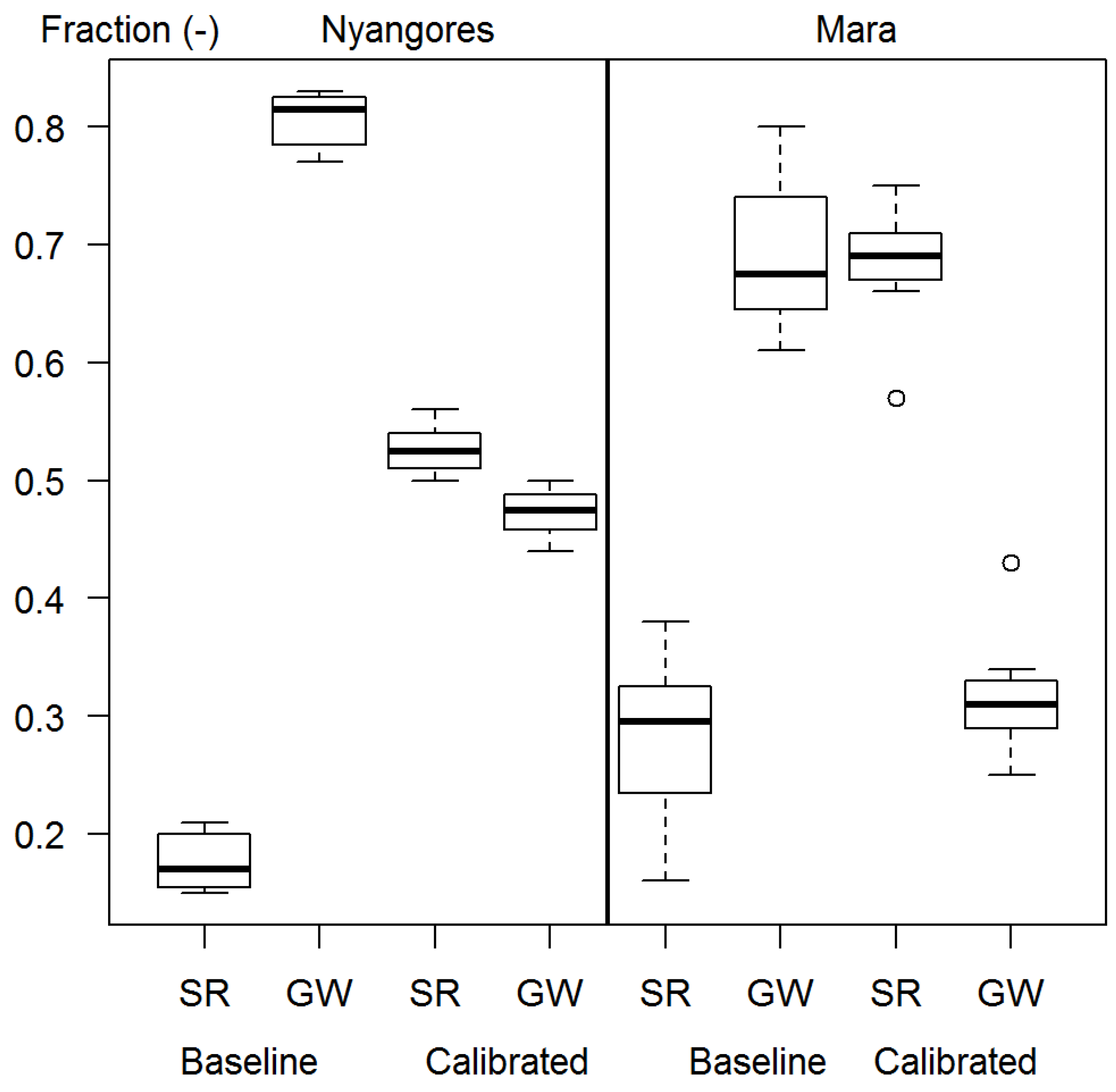
Figure 17 compares the contributions of surface runoff and subsurface streamflow to the total water yield annually for the Nyangores (W1) and Mara (W6) Rivers as simulated by the baseline and calibrated models. The baseline model exhibits a dominance of the subsurface flow contribution to the streamflow at both locations. In contrast, the calibrated model exhibits a comparable contribution of water from both the surface and subsurface components for the Nyangores River and surface runoff domination for the Mara River (Figure 17). On average, the surface runoff and subsurface flow contributions to the total water yield in the Nyangores (Mara) River are about 53% (68%) and 47% (32%), respectively. Given the physical characteristics of these watersheds (land use, soil and climate) shown in Table 1, we would expect differences in the dominant streamflow response behavior for the two watersheds. In theory, for a humid watershed (i.e., W1) with a moderate infiltration rate and a predominant evergreen forest cover, the surface runoff and subsurface flow contributions to the total water yield should be comparable. In contrast, the surface runoff contribution should dominate over the subsurface flow contribution for a semi-arid watershed (i.e., W6) with a moderate to low infiltration rate and a predominant savanna grassland cover. By these standards, the calibrated model shows both realistic and consistent watershed response behaviors when constrained using observed historical streamflow signatures and remote sensing-based evapotranspiration in a multi-objective framework. Our observations are consistent with Coxon et al. [66] and Yadav et al. [12], who demonstrated the dependence of the information content of diagnostics and its ability to constrain catchment response on catchment characteristics. The annual basin-level rainfall, evapotranspiration and water yield range from 951 to 1274 mm/year, 805 to 916 mm/year and 141 to 341 mm/year, respectively, for 2002–2009 (Figure S6). On average (2002–2009), the total water yield accounts for 24% of 1605 mm (W1: the Nyangores watershed at Bomet) and 21% of 1117 mm (W6: the Mara Basin at Mara Mines) of the input rainfall, whereas evapotranspiration accounts for 68% (W1) and 70% (W6). Our results agree with Dessu and Melesse [48], who reported the partitioning of the Mara Basin average rainfall as 70% evapotranspiration and 17% water yield.
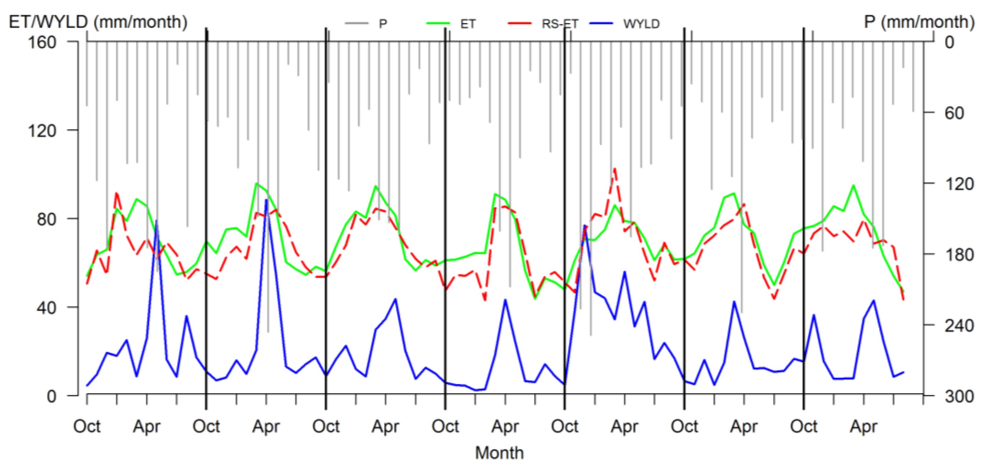
Figure 18 presents the monthly evapotranspiration and water yield dynamics in a hydrological year as simulated by the calibrated SWAT model for the Mara River. The water balance components reflect the rainfall seasonality well, with high water yields in April and August. However, the calibrated model shows limitations in representing the average watershed remote sensing-based evapotranspiration for the Nyangores watershed (W1) (see Figure S5).

7. Conclusions

We have presented a framework to calibrate and evaluate a hydrologic model for a poorly gauged basin. The core contribution is a demonstration of how to innovatively combine historical in situ streamflow observations with more recent remote sensing-based evapotranspiration to constrain a distributed hydrologic model within a multi-objective framework. Calibrating the SWAT model using multiple streamflow signatures derived from a normalized FDC reduced the biases in the simulated streamflow signatures considerably (above 25%) compared to the baseline (benchmark) model. The addition of the remote sensing-based evapotranspiration to the streamflow signatures to constrain the SWAT model further reduced the biases in the simulated streamflow signatures and improved the correlation of evapotranspiration (up to 25%) for the evergreen forest, savanna grassland and shrubland land cover classes. Our results highlight the potential of historical streamflow signature information and remote sensing-based evapotranspiration to effectively constrain different parts of the simulated streamflow regimes and evapotranspiration estimates. Even though rigorous model evaluation is limited, the formulated methodology contributes to the ongoing efforts to improve the modeling of poorly gauged and ungauged basins. We acknowledge the need for further application of the framework in different regions and more rigorous work on automatic multi-objective calibration with a sufficient number of function evaluations.

Supplementary Materials

The following supporting information can be downloaded at: https://www.mdpi.com/article/10.3390/w14081252/s1, Figure S1: The trade-off in evaluation criterion in a constrained search using Borg MOEA for the head water region (MM) based on streamflow signatures and RS-ET. Figure S2: Trade-off in two evaluation criterion spaces for the head water region (MM). Figure S3: Performance summary of the SWAT model for simulating the daily streamflow (2002–2007) using 13 Pareto set pa-rameters. Figure S4: Comparison of relative performances using SWAT model calibrated based on streamflow signature measures only (FDC) as reference for streamflow signature bias measures at the Nyangores and the Mara Rivers, and for evapotranspiration using correlation and percent of bias. Figure S5: The monthly water balance dynamics for 2002–2009 over the Nyangores watershed (HW) as simulated by SWAT. Figure S6: Simulated annual water balance for 2002–2009 over the Mara River Basin.

Author Contributions

Conceptualization, T.A., H.V.G. and A.v.G.; methodology, T.A. and H.V.G.; data curation, T.A.; writing—original draft preparation, T.A.; writing—review and editing T.A., H.V.G., A.v.G. and W.B.; visualization, T.A.; supervision, A.v.G. and W.B. All authors have read and agreed to the published version of the manuscript.

Funding

We would like to thank the Research Foundation—Flanders (FWO) for the travel grant to T. Alemayehu (V400616N) to conduct part of this research at the University of Arizona, Department of Hydrology and Water Resources. The authors thank the Research Foundation—Flanders (FWO) for funding the International Coordination Action (ICA) “Open Water Network: Open Data and Software tools for water resources management” (project code G0E2621N), the Flemish Research Council (VLIR) for funding the JOINT project “Global Open Water Academic Network: Joint Research and Education on Open Source Software for Integrated Water Resources Management” (project code TZ2019JOI022A105) and the EU H2020 program for funding “Water-ForCE—Water scenarios For Copernicus Exploitation” (grant agreement No. 101004186).

Informed Consent Statement

Not applicable.

Data Availability Statement

The remote sensing-based evapotranspiration data can be obtained from the first author upon request.

Acknowledgments

We also thank the Water Resource Management Authority (WRMA) of Kenya for providing streamflow data. The technical help from David Hadka, Penn State University, in customizing the Borg MOEA and SWAT using the R programming language environment is very much appreciated.

Conflicts of Interest

The authors declare no conflict of interest.

References

  1. Arnold, J.G.; Youssef, M.A.; Yen, H.; White, M.J.; Sheshukov, A.Y.; Sadeghi, A.M.; Moriasi, D.N.; Steiner, J.L.; Amatya, D.M.; Skaggs, R.W.; et al. Hydrological Processes and Model Representation: Impact of Soft Data on Calibration. Trans. ASABE 2015, 58, 1637–1660. [Google Scholar] [CrossRef]
  2. Clark, M.P.; Schaefli, B.; Schymanski, S.J.; Samaniego, L.; Luce, C.H.; Jackson, B.M.; Freer, J.E.; Arnold, J.R.; Moore, R.D.; Istanbulluoglu, E.; et al. Improving the theoretical underpinnings of process-based hydrologic models. Water Resour. Res. 2016, 52, 2350–2365. [Google Scholar] [CrossRef] [Green Version]
  3. Grayson, R.; Blöschl, G. Spatial modelling of catchment dynamics. In Spatial Patterns in Catchment Hydrology: Observations and Modelling; Cambridge Univ. Press: Cambridge, UK, 2000; pp. 51–81. ISBN 0521633168. [Google Scholar]
  4. Breuer, L.; Huisman, J.A.; Willems, P.; Bormann, H.; Bronstert, A.; Croke, B.F.W.; Frede, H.-G.; Gräff, T.; Hubrechts, L.; Jakeman, A.J.; et al. Assessing the impact of land use change on hydrology by ensemble modeling (LUCHEM). I: Model intercomparison with current land use. Adv. Water Resour. 2009, 32, 129–146. [Google Scholar] [CrossRef]
  5. Smith, M.B.; Seo, D.-J.; Koren, V.I.; Reed, S.M.; Zhang, Z.; Duan, Q.; Moreda, F.; Cong, S. The distributed model intercomparison project (DMIP): Motivation and experiment design. J. Hydrol. 2004, 298, 4–26. [Google Scholar] [CrossRef]
  6. Teklesadik, A.D.; Alemayehu, T.; van Griensven, A.; Kumar, R.; Liersch, S.; Eisner, S.; Tecklenburg, J.; Ewunte, S.; Wang, X. Inter-model comparison of hydrological impacts of climate change on the Upper Blue Nile basin using ensemble of hydrological models and global climate models. Clim. Change 2017, 141, 517–532. [Google Scholar] [CrossRef]
  7. Winsemius, H.C.; Savenije, H.H.G.; Bastiaanssen, W.G.M. Constraining model parameters on remotely sensed evaporation: Justification for distribution in ungauged basins? Hydrol. Earth Syst. Sci. Discuss. 2008, 5, 2293–2318. [Google Scholar] [CrossRef] [Green Version]
  8. Donnelly, C.; Andersson, J.C.M.; Arheimer, B. Using flow signatures and catchment similarities to evaluate the E-HYPE multi-basin model across Europe. Hydrol. Sci. J. 2016, 61, 255–273. [Google Scholar] [CrossRef]
  9. Euser, T.; Winsemius, H.C.; Hrachowitz, M.; Fenicia, F.; Uhlenbrook, S.; Savenije, H.H.G. A framework to assess the realism of model structures using hydrological signatures. Hydrol. Earth Syst. Sci. 2013, 17, 1893–1912. [Google Scholar] [CrossRef] [Green Version]
  10. Westerberg, I.K.; Guerrero, J.-L.; Younger, P.M.; Beven, K.J.; Seibert, J.; Halldin, S.; Freer, J.E.; Xu, C.-Y. Calibration of Hydrological Models Using Flow-Duration Curves. Hydrol. Earth Syst. Sci. 2011, 15, 2205–2227. [Google Scholar] [CrossRef] [Green Version]
  11. Winsemius, H.C.; Schaefli, B.; Montanari, A.; Savenije, H.H.G. On the Calibration of Hydrological Models in Ungauged Basins: A Framework for Integrating Hard and Soft Hydrological Information. Water Resour. Res. 2009, 45, 45. [Google Scholar] [CrossRef] [Green Version]
  12. Yadav, M.; Wagener, T.; Gupta, H. Regionalization of Constraints on Expected Watershed Response Behavior for Improved Predictions in Ungauged Basins. Adv. Water Resour. 2007, 30, 1756–1774. [Google Scholar] [CrossRef]
  13. Yilmaz, K.K.; Gupta, H.V.; Wagener, T. A Process-Based Diagnostic Approach to Model Evaluation: Application to the NWS Distributed Hydrologic Model. Water Resour. Res. 2008, 44, 1–18. [Google Scholar] [CrossRef] [Green Version]
  14. Gupta, H.V.; Wagener, T.; Liu, Y. Reconciling theory with observations: Elements of a diagnostic approach to model evaluation. Hydrol. Process. 2008, 22, 3802–3813. [Google Scholar] [CrossRef]
  15. Hrachowitz, M.; Savenije, H.H.G.; Blöschl, G.; McDonnell, J.J.; Sivapalan, M.; Pomeroy, J.W.; Arheimer, B.; Blume, T.; Clark, M.P.; Ehret, U.; et al. A decade of Predictions in Ungauged Basins (PUB)—A review. Hydrol. Sci. J. 2013, 58, 1198–1255. [Google Scholar] [CrossRef]
  16. Hrachowitz, M.; Fovet, O.; Ruiz, L.; Euser, T.; Gharari, S.; Nijzink, R.; Freer, J.; Savenije, H.H.G.; Gascuel-Odoux, C. Process consistency in models: The importance of system signatures, expert knowledge, and process complexity. Water Resour. Res. 2014, 50, 7445–7469. [Google Scholar] [CrossRef] [Green Version]
  17. Montanari, A.; Toth, E. Calibration of hydrological models in the spectral domain: An opportunity for scarcely gauged basins? Water Resour. Res. 2007, 43, 1–10. [Google Scholar] [CrossRef] [Green Version]
  18. Pauwels, V.R.N.; De Lannoy, G.J.M. Multivariate calibration of a water and energy balance model in the spectral domain. Water Resour. Res. 2011, 47. [Google Scholar] [CrossRef] [Green Version]
  19. Pfannerstill, M.; Guse, B.; Fohrer, N. Smart low flow signature metrics for an improved overall performance evaluation of hydrological models. J. Hydrol. 2014, 510, 447–458. [Google Scholar] [CrossRef]
  20. Pfannerstill, M.; Bieger, K.; Guse, B.; Bosch, D.D.; Fohrer, N.; Arnold, J.G. How to Constrain Multi-Objective Calibrations of the SWAT Model Using Water Balance Components. JAWRA J. Am. Water Resour. Assoc. 2017, 53, 532–546. [Google Scholar] [CrossRef]
  21. Shafii, M.; Tolson, B.A. Optimizing hydrological consistency by incorporating hydrological signatures into model calibration objectives. Water Resour. Res. 2015, 51, 3796–3814. [Google Scholar] [CrossRef] [Green Version]
  22. Smakhtin, V.U. Low flow hydrology: A review. J. Hydrol. 2001, 240, 147–186. [Google Scholar] [CrossRef]
  23. Vogel, R.M.; Fennessey, N.M. Flow-Duration Curves. I: New Interpretation and Confidence Intervals. J. Water Resour. Plan. Manag. 1994, 120, 485–504. [Google Scholar] [CrossRef]
  24. Boegh, E.; Thorsen, M.; Butts, M.B.; Hansen, S.; Christiansen, J.S.; Abrahamsen, P.; Hasager, C.B.; Jensen, N.O.; van der Keur, P.; Refsgaard, J.C.; et al. Incorporating remote sensing data in physically based distributed agro-hydrological modelling. J. Hydrol. 2004, 287, 279–299. [Google Scholar] [CrossRef]
  25. Boegh, E.; Poulsen, R.N.; Butts, M.; Abrahamsen, P.; Dellwik, E.; Hansen, S.; Hasager, C.B.; Ibrom, A.; Loerup, J.K.; Pilegaard, K.; et al. Remote sensing based evapotranspiration and runoff modeling of agricultural, forest and urban flux sites in Denmark: From field to macro-scale. J. Hydrol. 2009, 377, 300–316. [Google Scholar] [CrossRef]
  26. Huffman, G.J.; Bolvin, D.T.; Nelkin, E.J.; Wolff, D.B.; Adler, R.F.; Gu, G.; Hong, Y.; Bowman, K.P.; Stocker, E.F. The TRMM Multisatellite Precipitation Analysis (TMPA): Quasi-Global, Multiyear, Combined-Sensor Precipitation Estimates at Fine Scales. J. Hydrometeorol. 2007, 8, 38–55. [Google Scholar] [CrossRef]
  27. Karimi, P.; Bastiaanssen, W.G.M. Spatial evapotranspiration, rainfall and land use data in water accounting—Part 1: Review of the accuracy of the remote sensing data. Hydrol. Earth Syst. Sci. 2015, 19, 507–532. [Google Scholar] [CrossRef] [Green Version]
  28. Kite, G.W.; Pietroniro, A. Remote sensing applications in hydrological modelling. Hydrol. Sci. J. 1996, 41, 563–591. [Google Scholar] [CrossRef]
  29. Lakshmi, V. The role of satellite remote sensing in the prediction of ungauged basins. Hydrol. Process. 2004, 18, 1029–1034. [Google Scholar] [CrossRef]
  30. Wagner, W.; Verhoest, N.E.C.; Ludwig, R.; Tedesco, M. Editorial “Remote sensing in hydrological sciences”. Hydrol. Earth Syst. Sci. 2009, 13, 813–817. [Google Scholar] [CrossRef] [Green Version]
  31. Immerzeel, W.W.; Droogers, P. Calibration of a distributed hydrological model based on satellite evapotranspiration. J. Hydrol. 2008, 349, 411–424. [Google Scholar] [CrossRef]
  32. Rientjes, T.H.M.; Muthuwatta, L.P.; Bos, M.G.; Booij, M.J.; Bhatti, H.a. Multi-variable calibration of a semi-distributed hydrological model using streamflow data and satellite-based evapotranspiration. J. Hydrol. 2013, 505, 276–290. [Google Scholar] [CrossRef]
  33. Zhang, Y.; Chiew, F.H.S.; Zhang, L.; Li, H. Use of Remotely Sensed Actual Evapotranspiration to Improve Rainfall–Runoff Modeling in Southeast Australia. J. Hydrometeorol. 2009, 10, 969–980. [Google Scholar] [CrossRef]
  34. Kunnath-Poovakka, A.; Ryu, D.; Renzullo, L.J.; George, B. The efficacy of calibrating hydrologic model using remotely sensed evapotranspiration and soil moisture for streamflow prediction. J. Hydrol. 2016, 535, 509–524. [Google Scholar] [CrossRef]
  35. Arnold, J.G.; Srinivasan, R.; Muttiah, R.S.; Williams, J.R. Large area hydrologic modeling and assessment part I: Model development. J. Am. Water Resour. Assoc. 1998, 34, 73–89. [Google Scholar] [CrossRef]
  36. KMD Kenya Meteorological Department. Available online: http://www.meteo.go.ke/data/ (accessed on 20 September 2014).
  37. Karimi, P.; Bastiaanssen, W.G.M.; Sood, A.; Hoogeveen, J.; Peiser, L.; Bastidas-Obando, E.; Dost, R.J. Spatial evapotranspiration, rainfall and land use data in water accounting—Part 2: Reliability of water acounting results for policy decisions in the Awash Basin. Hydrol. Earth Syst. Sci. 2015, 19, 533–550. [Google Scholar] [CrossRef] [Green Version]
  38. Juston, J.; Jansson, P.; Gustafsson, D. Rating curve uncertainty and change detection in discharge time series: Case study with 44-year historic data from the Nyangores River, Kenya. Hydrol. Process. 2013, 28, 2509–2523. [Google Scholar] [CrossRef]
  39. McClain, M.E.; Subalusky, A.L.; Anderson, E.P.; Dessu, S.B.; Melesse, A.M.; Ndomba, P.M.; Mtamba, J.O.D.; Tamatamah, R.A.; Mligo, C. Comparing flow regime, channel hydraulics, and biological communities to infer flow–ecology relationships in the Mara River of Kenya and Tanzania. Hydrol. Sci. J. 2014, 59, 801–819. [Google Scholar] [CrossRef]
  40. WREM. Mara River Basin Monograph, Mara River Basin Transboundary Integrated Water Resources Management and Development Project, Final Technical Report; WREM International Inc.: Atlanta, GA, USA, 2008. [Google Scholar]
  41. Gereta, E.; Mwangomo, E.; Wolanski, E. Ecohydrology as a tool for the survival of the threatened Serengeti ecosystem. Ecohydrol. Hydrobiol. 2009, 9, 115–124. [Google Scholar] [CrossRef]
  42. Neitsch, S.L.; Arnold, J.G.; Kiniry, J.R.; Williams, J.R. Soil & Water Assessment Tool Theoretical Documentation Version 2009; Texas Water Resources Institute Technical Report No. 406; Texas A&M University: College Station, TX, USA, 2011; p. 647. [Google Scholar]
  43. Alemayehu, T.; van Griensven, A.; Woldegiorgis, B.T.; Bauwens, W. An improved SWAT vegetation growth module and its evaluation for four tropical ecosystems. Hydrol. Earth Syst. Sci. 2017, 21, 4449–4467. [Google Scholar] [CrossRef] [Green Version]
  44. Nachtergaele, F.O.; van Velthuizen, H.; Verelst, L.; Batjes, N.H.; Dijkshoorn, J.A.; van Engelen, V.W.P.; Fischer, G.; Jones, A.; Montanarella, L.; Petri, M.; et al. Harmonized World Soil Database (Version 1.0); Food and Agric Organization of the UN (FAO): Rome, Italy; International Inst. for Applied Systems Analysis (IIASA): Laxenburg, Austria; ISRIC—World Soil Information: Bengaluru, India; Inst of Soil Science-Chinese Acad of Sciences (ISS-CAS): Lausanne, Switzerland; EC-Joint Research Centre (JRC): Ispra, Italy, 2008. [Google Scholar]
  45. Roy, T.; Serrat-Capdevila, A.; Gupta, H.; Valdes, J. A platform for probabilistic Multimodel and Multiproduct Streamflow Forecasting. Water Resour. Res. 2017, 53, 376–399. [Google Scholar] [CrossRef] [Green Version]
  46. Rodell, M.; Houser, P.R.; Jambor, U.; Gottschalck, J.; Mitchell, K.; Meng, C.-J.; Arsenault, K.; Cosgrove, B.; Radakovich, J.; Bosilovich, M.; et al. The Global Land Data Assimilation System. Bull. Am. Meteorol. Soc. 2004, 85, 381–394. [Google Scholar] [CrossRef] [Green Version]
  47. Alemayehu, T.; Griensven, A.V.; Bauwens, W. Evaluating CFSR and WATCH Data as Input to SWAT for the Estimation of the Potential Evapotranspiration in a Data-Scarce Eastern-African Catchment. J. Hydrol. Eng. 2016, 21, 05015028. [Google Scholar] [CrossRef]
  48. Dessu, S.B.; Melesse, A.M. Modelling the rainfall-runoff process of the Mara River basin using the Soil and Water Assessment Tool. Hydrol. Process. 2012, 26, 4038–4049. [Google Scholar] [CrossRef]
  49. Mango, L.M.; Melesse, A.M.; McClain, M.E.; Gann, D.; Setegn, S.G. Land use and climate change impacts on the hydrology of the upper Mara River Basin, Kenya: Results of a modeling study to support better resource management. Hydrol. Earth Syst. Sci. 2011, 15, 2245–2258. [Google Scholar] [CrossRef] [Green Version]
  50. Mwangi, H.M.; Julich, S.; Patil, S.D.; McDonald, M.A.; Feger, K.-H. Modelling the impact of agroforestry on hydrology of Mara River Basin in East Africa. Hydrol. Process. 2016, 30, 3139–3155. [Google Scholar] [CrossRef] [Green Version]
  51. Alemayehu, T.; Griensven, A.V.; Senay, G.B.; Bauwens, W. Evapotranspiration Mapping in a Heterogeneous Landscape Using Remote Sensing and Global Weather Datasets: Application to the Mara Basin, East Africa. Remote Sens. 2017, 9, 390. [Google Scholar] [CrossRef] [Green Version]
  52. Senay, G.B.; Bohms, S.; Singh, R.K.; Gowda, P.H.; Velpuri, N.M.; Alemu, H.; Verdin, J.P. Operational Evapotranspiration Mapping Using Remote Sensing and Weather Datasets: A New Parameterization for the SSEB Approach. J. Am. Water Resour. Assoc. 2013, 49, 577–591. [Google Scholar] [CrossRef] [Green Version]
  53. Jung, M.; Reichstein, M.; Margolis, H.A.; Cescatti, A.; Richardson, A.D.; Arain, M.A.; Arneth, A.; Bernhofer, C.; Bonal, D.; Chen, J.; et al. Global patterns of land-atmosphere fluxes of carbon dioxide, latent heat, and sensible heat derived from eddy covariance, satellite, and meteorological observations. J. Geophys. Res. 2011, 116, G00J07. [Google Scholar] [CrossRef] [Green Version]
  54. Hadka, D.; Reed, P. Borg: An Auto-Adaptive Many-Objective Evolutionary Computing Framework. Evol. Comput. 2013, 21, 231–259. [Google Scholar] [CrossRef]
  55. Reed, P.M.; Hadka, D.; Herman, J.D.; Kasprzyk, J.R.; Kollat, J.B. Evolutionary multiobjective optimization in water resources: The past, present, and future. Adv. Water Resour. 2013, 51, 438–456. [Google Scholar] [CrossRef] [Green Version]
  56. Hadka, D.; Herman, J.; Reed, P.; Keller, K. An open source framework for many-objective robust decision making. Environ. Model. Softw. 2015, 74, 114–129. [Google Scholar] [CrossRef] [Green Version]
  57. Wagener, T. Evaluation of catchment models. Hydrol. Process. 2003, 17, 3375–3378. [Google Scholar] [CrossRef]
  58. Budyko, M.I. Climate and Life; Academic Press: San Diego, CA, USA, 1974. [Google Scholar]
  59. Du, C.; Sun, F.; Yu, J.; Liu, X.; Chen, Y. New interpretation of the role of water balance in an extended Budyko hypothesis in arid regions. Hydrol. Earth Syst. Sci. 2016, 20, 393–409. [Google Scholar] [CrossRef] [Green Version]
  60. Troch, P.A.; Carrillo, G.; Sivapalan, M.; Wagener, T.; Sawicz, K. Climate-vegetation-soil interactions and long-term hydrologic partitioning: Signatures of catchment co-evolution. Hydrol. Earth Syst. Sci. 2013, 17, 2209–2217. [Google Scholar] [CrossRef] [Green Version]
  61. Zhang, L.; Hickel, K.; Dawes, W.R.; Chiew, F.H.S.; Western, A.W.; Briggs, P.R. A rational function approach for estimating mean annual evapotranspiration. Water Resour. Res. 2004, 40, 89–97. [Google Scholar] [CrossRef]
  62. Fu, B.P. On the calculation of the evaporation from land surface. Sci. Atmos. Sin. 1981, 5, 23–31. (In Chinese) [Google Scholar]
  63. Gupta, H.V.; Sorooshian, S.; Yapo, P.O. Toward improved calibration of hydrologic models: Multiple and noncommensurable measures of information. Water Resour. Res. 1998, 34, 751–763. [Google Scholar] [CrossRef]
  64. Marshall, M.T.; Funk, C. Agricultural Drought Monitoring in Kenya Using Evapotranspiration Derived from Remote Sensing and Reanalysis Data. In Remote Sensing of Drought: Innovative Monitoring Approaches; Wardlow, B.D., Anderson, M.C., Verdin, J.P., Eds.; CRC Press: Boca Raton, FL, USA, 2012; pp. 169–194. [Google Scholar]
  65. Rulinda, C.M.; Dilo, A.; Bijker, W.; Stein, A. Characterising and quantifying vegetative drought in East Africa using fuzzy modelling and NDVI data. J. Arid Environ. 2012, 78, 169–178. [Google Scholar] [CrossRef]
  66. Coxon, G.; Freer, J.; Wagener, T.; Odoni, N.A.; Clark, M. Diagnostic evaluation of multiple hypotheses of hydrological behaviour in a limits-of-acceptability framework for 24 UK catchments. Hydrol. Process. 2014, 28, 6135–6150. [Google Scholar] [CrossRef]
Figure 1. Streamflow data availability for the Nyangores River at Bomet station (1LA03) and the Mara River at Mines station (5H2).
Water 14 01252 g001
Figure 2. The location of the Mara Basin in East Africa. Selected sample watersheds with varying aridity and landscape characteristics are marked with W1–W6. The inset map shows the boundary of Kenya and Tanzania.
Water 14 01252 g002
Figure 3. A schematic of the workflow used in this study.
Water 14 01252 g003
Figure 4. Flow duration curves using normalized daily streamflow (1970–1990) for the Nyangores River at ILA03 (a). Parts of the FDC used in this study to derive the streamflow signature information (b). Note that the daily streamflow is normalized with the mean annual streamflow.
Water 14 01252 g004
Figure 5. Comparison of normalized mean annual flow duration curves for simulated (2002–2007) and observed (1970–1990) streamflow for the Nyangores River at Bomet (a) and the Mara River at Mara Mines (b) using different calibration strategies: uncalibrated (baseline), manually calibrated using only streamflow signatures (FDC) and coupled with evapotranspiration (FDC + ET), automatic multi-objective calibration (bestMO). Note that the y-axis is in log scale.
Water 14 01252 g005
Figure 6. A comparison of the performance measures for simulated (2002–2007) coupled with observed historical (1970–1990) streamflow signatures for the Nyangores River at Bomet (a) and the Mara River at Mara Mines (b). BFHV and BFLV denote biases in the high- and low-streamflow regimes, respectively; BFMS represents the bias in the slope of the flow duration curve.
Water 14 01252 g006
Figure 7. Comparison of 8-day simulated and remote sensing-based evapotranspiration annually (2002–2007) for evergreen forest (FRSE), savanna grassland (RNGE) and shrubland (RNGB) using boxplots: (a) percent of bias (pbias) and (b) correlation coefficient (r).
Water 14 01252 g007
Figure 8. The trade-off in evaluation criteria in a constrained search using the Borg MOEA for sub-basins 1–18 based on streamflow signatures and remote sensing-based evapotranspiration during the calibration period (2002–2007). The location where the line intersects each vertical axis designates the relative objective value. The gray lines represent the efficiency measures in the provided parameter space (MO (constrained)), while the solid black line represents the selected best trade-off (BestMO) from the Pareto solution set. Note that the correlation coefficient is defined as 1−r.
Water 14 01252 g008
Figure 9. Trade-off in two evaluation criterion spaces for sub-basins 1–18 during the calibration period (2002–2007). The gray dots show all the evaluations in the constrained search (MO (constrained)); the black dots (Bestpareto) represent the best trade-off for the respective bi-criteria with a bias lower than 5% and a correlation higher than 0.65. The upward triangle and downward triangle markers denote evaluations for the baseline and manually calibrated models (FDC + ET), respectively. The square marker represents the selected best trade-off taking into account all the objectives (BestMO).
Water 14 01252 g009
Figure 10. Mean annual FDCs (2002–2007) using the selected Pareto set solutions for the Nyangores River at Bomet (a) and the Mara River at Mines (b).
Water 14 01252 g010
Figure 11. Daily simulated and observed streamflow comparisons for the Nyangores River at Bomet. Top panel: the range based on the 13 selected Pareto set solutions (ParetoRange); bottom panel: simulated streamflow based on manual calibration using evapotranspiration and signature measures.
Water 14 01252 g011
Figure 12. Budyko diagram based on the annual (a) and the mean annual (b) rainfall (P), evapotranspiration (ET) and reference evapotranspiration (ET0) estimates across several watersheds (W1–W6). The solid lines show the Fu curves for w values of 2.6 and 2.0.
Water 14 01252 g012
Figure 13. (a) The correlation between the optimized Fu w values and the runoff coefficient (WYLD/P) across several watersheds. (b) The correlation between the mean annual runoff coefficient and the evaporative index (ET/P). Note that this illustration is derived from Figure 12.
Water 14 01252 g013
Figure 14. The relative performance of calibrated SWAT compared to the baseline model for streamflow signature bias measures for the Nyangores (a) and Mara (b) Rivers, and for evapotranspiration using correlation (c) and percent of bias (d). FDC: calibration using only streamflow signature measures; FDC + ET: calibration using streamflow signature measures and remote sensing-based evapotranspiration; BestMO: automatic multi-objective calibration based on the selected best parameter set from the Pareto set solutions.
Water 14 01252 g014
Figure 15. Daily mean basin soil water dynamics as simulated by the baseline and calibrated SWAT models (2002–2007). FDC: calibration using only streamflow signature measures; FDC+ET: calibration using streamflow signature measures and remote sensing evapotranspiration; BestMO: automatic multi-objective calibration based on selected best parameter set from the Pareto set solutions.
Water 14 01252 g015
Figure 16. Spatial distribution of the SWAT simulated soil water content at the HRU level for 5 May 2002: (a) calibrated using streamflow signatures (FDC); (b) calibrated using streamflow signatures and ET-RS (FDC+ET); and (c) the difference between the two (b–a).
Water 14 01252 g016
Figure 17. The surface runoff (SR) and groundwater flow (GW) contributions to the total water yield as simulated by the SWAT models.
Water 14 01252 g017
Figure 18. The monthly water balance dynamics for 2002–2009 over the Mara Mines watershed (W6) as simulated by SWAT. The months are arranged according to the hydrological year (Oct–Sept).
Water 14 01252 g018
Table 1. Summary of selected watershed characteristics. P, ET0 and ET represent mean annual (2002–2009) rainfall and reference and actual evapotranspiration, respectively. See their location in Figure 2 and note that W1 and W6 are watersheds with gauging stations.
Watershed IDArea
(km2)
Elevation
(m.a.s.l.)
Dominant Land CoverDominant Soil TypeP
(mm)
ET0
(mm)
ET
(mm)
Aridity Index
W16912397Forest (63%)Andosols (100%)1605149410310.94
W26952684Forest (45%)Andosols (100%)142814528971.03
W313921507Grassland (79%)Luvic Phaeozems (67%)81116567032.12
W43861892Grassland (92%)Eutric Planosols (62%) 123817399191.42
W56221292Wetland (40%)Eutric Planosols (56%)144617109531.19
W611,2851811Grassland (60%)Planosols (19%)111716588351.50
Basin13,4221729Grassland (35%)Eutric Planosols (40%)115316668451.46
Table 2. The list of SWAT parameters used during model calibration with their range.
ParameterFunction (Unit)Variation LevelRange aAdjustment b
MinMax
SOL_ZSoil depths (mm)HRU2402000R
SOL_AWCSoil water content (mm)HRU00.45R
SOL_KSoil hydraulic conductivity (mm/h)HRU067.6R
ESCOSoil evaporation (-)HRU01V
EPCOPlant water uptake (-)HRU01V
REVAPMNDepth of water in the aquifer for “revap” (mm)Watershed0200V
CN2Surface runoff (-)HRU2598R
SURLAGSurface runoff routing (day)HRU0.0110V
ALPHA_BFBaseflow recession constant (day)Watershed01V
GWQMNShallow aquifer minimum level for baseflow (mm)Watershed0500V
GW_REVAPGroundwater “revap” coefficient (-)Watershed0.020.2V
RCHRG_DPDeep aquifer percolation (-)Watershed01V
GW_DELAYGroundwater delay (day)Watershed0100V
CANMXInterception storage (mm)Land cover06R
a Parameter value range that is set after manual adjustment for automatic calibration; b type of change to be applied to parameters during calibration: R means an existing parameter value is multiplied by an adjustment factor, and V means a current parameter value is replaced by a given value.
Table 3. Performance metrics for the simulated evapotranspiration during the validation period (2008–2009). Legend: FRSE = evergreen forest; RNGE = savanna grassland; RNGB = shrubland.
FRSE RNGE RNGB
pbiasrpbiasrpbiasr
FDC3.50.1212.70.755.80.73
FDC + ET14.30.6712.50.764.90.73
BestMO12.10.6416.90.817.20.78
Table 4. Summary statistics for the simulated and observed mean annual streamflow duration curves (in m3/s) for 2008–2009.
Nyangores RiverMara River
Historical 1FDCFDC + ETBestMOHistorical 1FDCFDC + ETBestMO
Min0.30.10.10.00.013.33.53.5
Median5.25.15.38.216.827.230.131.8
IQR7.87.06.910.030.337.040.833.2
Max52.350.847.382.0655459517546
1 Based on historical available daily observed streamflow (1970–1990).
Table 5. Calibrated SWAT parameters using streamflow signatures (FDC), streamflow signatures and remote sensing-based evapotranspiration (FDC + ET) and automatic multi-objective calibration (Pareto range).
Sub-Basins 1–18Sub-Basins 19–89
FDCFDC+ETPareto RangeFDCFDC+ETPareto Range
ParameterAdjustment MinMax MinMax
SOL_ZR0.000.60−0.051.000.000.60−0.200.35
SOL_AWCR−0.21−0.18−0.400.40−0.21−0.18−0.120.18
GW_REVAPV0.020.170.020.200.020.020.020.08
GWQMNV150.00150.0049.88278.22100.00100.00157.20462.10
RCHRG_DPV0.700.700.000.520.100.100.000.46
SOL_KR−0.20−0.20−0.300.29−0.20−0.20−0.300.30
REVAPMNV500.00100.0090.00177.41500.00100.00136.20168.30
ALPHA_BFV0.900.900.000.900.020.020.040.89
SURLAGV0.100.100.002.000.350.350.901.93
CN2R−0.33−0.33−0.350.060.140.14−0.100.09
ESCOV0.950.980.000.960.950.980.001.00
EPCOV1.001.000.001.001.001.000.021.00
GW_DELAYV15.0015.0015.0046.1760.0060.0045.5060.00
CANMXR −0.80 −0.80
Publisher’s Note: MDPI stays neutral with regard to jurisdictional claims in published maps and institutional affiliations.