Abstract
Surface water quality management is an important facet of the effort to meet increasing demand for water. For that purpose, water quality must be monitored and assessed via the use of innovative techniques, such as water quality indices (WQIs), spectral reflectance indices (SRIs), and multivariate modeling. Throughout the Rosetta and Damietta branches of the Nile River, water samples were collected, and WQIs were assessed at 51 different distinct locations. The drinking water quality index (DWQI), metal index (MI), pollution index (PI), turbidity (Turb.) and total suspended solids (TSS) were assessed to estimate water quality status. Twenty-three physicochemical parameters were examined using standard analytical procedures. The average values of ions and metals exhibited the following sequences: Ca2+ > Na2+ > Mg2+ > K+, HCO32− > Cl− > SO42− > NO3− > CO3− and Al > Fe > Mn > Ba > Ni > Zn > Mo > Cr > Cr, respectively. Furthermore, under the stress of evaporation and the reverse ion exchange process, the main hydrochemical facies were Ca-HCO3 and mixed Ca-Mg-Cl-SO4. The DWQI values of the two Nile branches revealed that 53% of samples varied from excellent to good water, 43% of samples varied from poor to very poor water, and 4% of samples were unsuitable for drinking. In addition, the results showed that the new SRIs extracted from VIS and NIR region exhibited strong relationships with DWQI and MI and moderate to strong relationships with Turb. and TSS for each branch of the Nile River and their combination. The values of the R2 relationships between the new SRIs and WQIs varied from 0.65 to 0.82, 0.64 to 0.83, 0.41 to 0.60 and 0.35 to 0.79 for DWQI, MI, Turb. and TSS, respectively. The PLSR model produced a more accurate assessment of DWQI and MI based on values of R2 and slope than other indices. Furthermore, the partial least squares regression model (PLSR) generated accurate predictions for DWQI and MI of the Rosetta branch in the Val. datasets with an R2 of 0.82 and 0.79, respectively, and for DWQI and MI of the Damietta branch with an R2 of 0.93 and 0.78, respectively. Therefore, the combination of WQIs, SRIs, PLSR and GIS approaches are effective and give us a clear picture for assessing the suitability of surface water for drinking and its controlling factors.
1. Introduction
The water supply is considered a fundamental requirement for human activity and socioeconomic utility, and is indispensable for human wellbeing. Rivers are the most often used sources of surface water due to their abundance and accessibility, which have led to rapid human population growth and progress near watercourses [,,]. Consequently, rivers particularly in developing nations have suffered from significant environmental pressures associated with contamination from intensive agricultural pesticide runoff and effluent from manufacturing processes, sewage, and other urban waste sources [,,].
As the essential freshwater source in Egypt, the Nile River receives large amounts of residential and agricultural waste, manufacturing pollutants, and municipal discharges, all of which degrade the river’s water quality [,,,,]. The metal sector contributes about 50% of the total in waste outflows, which, together with industrial effluents as well as agricultural runoff and municipal sewage, constitute serious hazards to the aquatic system in the Nile River [,]. Therefore, the contamination of the Nile River has been regarded as one of Egypt’s most critical water-related issues, particularly since the recent construction of the Ethiopia Dam, which led to significant environmental and human health problems [,]. Therefore, water quality monitoring and water resource management have been accepted as a national duty for achieving sustainability in Egypt.
Water quality is evaluated using physical and chemical properties that indicate water characteristics and variables that impact on water quality []. Hence, physicochemical parameters based on hydrochemical metrics provide an initial understanding of water facies, numerous geochemical mechanisms, and water categorization [,,]. Moreover, water quality indices (WQIs) are among the better approaches to explain water quality [,], as they convert original data from many water quality metrics into a single number to understand water quality as a whole at different monitoring points at a given time [,,,] and assist strategic planning linked to water quality management programs through numerical index values [,,]. Therefore, the indices used in this study, namely the drinking water quality index (DWQI), metal index (MI), and pollution index (PI), were determined to assess water quality.
In the last decades, multivariate statistical approaches such as cluster analysis (CA) and principal component analysis (PCA) have been used extensively to arrange and clarify information and describe the quality of the water [,,,,,]. They are commonly utilized in water quality monitoring and evaluation [,,,]. The multivariate approach can assist in classifying the investigated characteristics into distinct categories depending on the influence from predicted sources and can offer insights about their genesis according to the variability of the investigated data []. Thus, the CA and PCA are efficient approaches for discovering common trends and anomalies of dispersion, reducing the initial dimension of datasets, and improving understanding of the geogenic and environmental origins of soluble ions and metals in water [,].
Estimates of DWQI, MI, Turb., and TSS have relied on point sampling and laboratory tests. This method is accurate, but it is slow, costly, harmful, and geographically limited, making it inefficient for monitoring these indices. It also cannot be utilized to help decision-makers with a complete assessment of critical indices related to water quality [,,,]. To help overcome this problem, WQIs can be monitored by remote sensing technology. With the rapid improvements in remote sensing techniques for collecting data, different UAV, satellite, or proximate hyperspectral tools have been proved to be economical and usable on a broad scale for integrative evaluation of many water quality indicators [,]. Compared to satellite images, proximate hyperspectral sensing could be a beneficial tool for overcoming the limitations imposed by external interference factors in monitoring and assessing quality. Because the optical sensors are close to the target, the system can collect high-resolution spectrum information and assure spectral inversion accuracy. This system’s information benefits from a large volume of data, huge bands, and high quantitative inversion flexibility []. The concept underlying these techniques is that the numerous sensors in these instruments can determine changes in the water surface’s optical properties at various bands. The changes in the physiochemical, biological, and hydrological aspects of the water are intricately related to the water surface’s optical properties. As a result, the spectra emitted by the water’s surface could be used directly or indirectly to estimate WQIs, such as Turb., TSS, total phosphorus, chlorophyll, irrigation water quality index, and dissolved organic carbon [,,,,,,,,]. Previous studies have discovered that there were close relationships between certain WQIs and water surface spectral reflectance in certain wavebands, particularly in the visible and near-infrared ranges. For example, Gitelson et al. [] found that the spectrum range in the 700–900 nm for remote sensing is the best range for estimating TSS concentrations. Spectral reflectance at 806 nm is strongly linked with the TSS of water (R2 = 0.89), according to Vincikova et al. []. Additionally, Elhag et al. [] found that water Turb. measurements revealed a strong relationship with calculated normalized differences in the Turb. index, with an R2 of 0.94. Although several studies focused on WQIs, there is limited evidence available to evaluate the SRI approaches to assess WQIs such as DWQI and MI. Therefore, this study also focused on evaluating the possibility of using published and new two-band spectral indices to estimate DWQI, MI, Turb., and TSS of surface water.
Because spectral measurements create a large amount of data, using a suitable statistical model to analyze spectral reflectance data remains a critical step in identifying the best association between spectral data and various water quality indicators. In addition to deriving algorithms created utilizing specific bands or band ratios, multivariate models based on numerous spectral bands or SRIs were shown to be an effective technique to estimate the different water quality indicators [,]. Since the PLSR can combine several types of spectral reflectance data as input variables, it was used to predict water quality indicators as output variables [,]. PLSR has been presented as a method for resolving strong multi-collinear and noisy factors in spectrum regions and assessing water quality indicators effectively []. In this way, PLSR may provide valuable information that supports the efficacy of spectral un-mixing techniques.
There are insufficient data to evaluate the benefits of using SRI-based PLSR models for predicting both the DWQI and MI of the Nile River’s water surface. Therefore, the goals of this work were to (1) explore surface water facies and numerous geochemical processes using physicochemical properties; (2) determine the geochemical regulating processes impacting water chemistry using imitative approaches; (3) assess the suitability of water samples for drinking using the DWQI; (4) assess the susceptibility of fresh water to pollution using MI and PI; (5) evaluate the performance of published and new SRIs to assess the four WQIs, namely DWQI, MI, Turb., and TSS, of Nile River surface water; and (6) evaluate the efficacy of PLSR models as quick approaches for predicting the four WQIs of the Nile River.
2. Materials and Methods
2.1. Study Area
The Nile River is regarded as one of the world’s longest rivers, with a total length of around 6700 km, including about 1352 km within Egypt. The Nile River flows 940 km upstream of the Aswan High Dam before splitting into two branches including the Rosetta and Damietta branches (Figure 1), which encompass around 12,357 km2 []. The Rosetta branch is approximately 225 km long, with a width of about 180 m, and has a depth ranging from 2 to 4 m; it begins in EL-Kanater El-Khayria in the south and ends at Rashid City in the north, whereas the fresh water of the Rosetta branch terminates at the Edfina Barrage 30 km upstream from the sea, which discharges excess water to the Mediterranean Sea via the Rosetta Estuary []. In addition, the Damietta branch is approximately 242 km long, with an average width of 200 m and an average depth of 12 m. The study region extends approximately 237.0 km from the delta barrage to the Rosetta and Damietta outflow [].
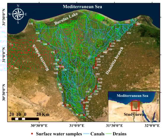
Figure 1.
The location map of the collected water samples and surface water network along Rosetta and Damietta branches.
2.2. Sampling and Analyses
During the year 2021, 51 surface water samples were collected along the Rosetta and Damietta branches during a surveying trip in the research region to collect data representing the overall actual conditions for determination of water quality for consumption and utilization. The locations of the obtained samples were determined in UTM positions using a portable Magellan GPS 315 (Figure 1). Two sets of collected water samples were stored in 500 mL plastic bottles and purified using 0.45 m Whatman filter paper. For metal analysis, samples were adjusted to pH = 2 using conc. HNO3 before being examined. The samples were kept at 4 °C once they were brought to the laboratories for chemical characterization. Using established analytical procedures [], 23 distinct physicochemical parameters were measured. Temperature, pH, EC, and TDS were detected in situ using a calibrated handheld conductivity multi-parameter sensor (Hanna HI 9033). The titrimetric technique was used to determine Ca2+ and Mg2+, Cl−, HCO3−, and CO32− concentrations. In addition, a flame photometer (ELEX 6361, Eppendorf AG, Hamburg, Germany) was used to measure the K+ and Na+ concentrations. The concentrations of SO42− and NO3− were determined using a spectrophotometer instrument with a visible ultraviolet spectrum (DR/2040—Loveland, CO, USA). The total suspended solids (TSS) were measured in mg/L by using a glass filter paper filtration technique. A turbidimeter measured the level of Turb. in water, which was stated in nephelometric turbidity units (NTU). Different quality assurance approaches were used throughout the water sample analysis. After the experimental data were double-checked in the lab, charge balance errors (CBE) were established, and samples were verified in triplicate, with the average value provided. An inductively coupled plasma mass spectrometer (ICP-MS, Thermo Fisher Scientific Inc., Mundelein, IL, USA) was used and standard analytical protocols [] were performed to examine metals (Al, Ba, Cr, Cu, Fe, Mn, Mo, Ni, and Zn).
2.3. Indexing Approach
Different approaches, which were governed by three factors including parameter selection, quality function calculation (sub-index), and accumulation of sub-indices, were applied using arithmetic equations and compared to evaluate the suitability of collected water samples along the Nile River for drinking [,,,]. The suitability of surface water for drinking and its sensitivity to pollution were investigated using the cited WQIs such as, DWQI, MI, and PI, which were calculated using physical and chemical properties.
2.3.1. Drinking Water Quality Index (DWQI)
For potable water quality assessment, the findings on 23 physicochemical parameters of collected samples were considered. The physical and chemical parameters were weighted based on their significance to the total quality of water. The DWQI reflects the total water quality of water variables based on a combination of water characteristics and their utilization in the ecosystem [], as indicated in Equation (1):
According to the WHO [], the estimated value of Qi is influenced by the concentration of each water component (Ci) and their guideline (Si) for drinking water, as indicated in Equation (2):
where Wi is the relative weight and wi is the weight unit of each water component.
Equation (4) is applied to determine wi for each component in accordance with the specified criteria for drinking water [].
wi = K/Si
K is the constant of proportionality, which can be computed using Equation (5):
To calculate DWQI, a weight for each surface water parameter (wi) was assigned for Turb., pH, TDS, EC, TH, K+, Na+, Mg2−, Ca2+, Cl−, SO42−, HCO32−, CO3−, NO3−, Al, Ba, Cr, Cu, Fe, Mn, Mo, Ni, and Zn, and the quality rating range (Qi) and relative weight (Wi) were estimated. The computed values of the standards, unit weights (wi) and relative weights (Wi) for the surface water parameters are showed in Table 1.

Table 1.
Calculation of the DWQI based on the arithmetic weight method for physicochemical parameters.
2.3.2. Pollution Indices (PIs)
The pollution indices, such as MI and PI, were calculated for the concentrations of metals including Al, Ba, Cr, Cu, Fe, Mn, Mo, Ni, and Zn using the formulae presented in Table 1.
Metal Index (MI)
According to Equation (6), the metal index (MI) was used to analyze the probable impact of metals on public health, which helps in swiftly estimating the overall quality of water [].
where Hc is a concentration of each metal in the collected water sample, Hmax is the max. limit concentration for each metal, and the subscript i is the i-th sample [].
Pollution Index (PI)
The PI values were used to evaluate the influence of metal pollution on surface water []. According to Equation (7), the PI is categorized into five groups (Table 2), which reflect the distinct pollution influence from each metal on water quality.
where Ci represents the content of each metal in the collected sample and Si represents the standard limit of each metal in potable water [,].
Table 2.
Levels of pollution according to PI values [].
2.4. Proximate Hyperspectral Measurements
The acquisition device was a handheld spectrometer (band range of 302–1148 nm; tec5 AG, Oberursel, Germany). It was used to acquire spectral reflectance measurements of surface water samples. The device is made up of two primary parts, one of which is attached to a diffuser and detects solar radiation, while the other component measures water samples’ spectral reflectance. Water samples were put in 25 cm diameter black cylindrical containers with a 10 cm depth, and the spectrometer optic was placed vertically around 25 cm at a nadir position over the water surface of the samples with a scanning area of 0.05 m2. The water samples’ spectral reflectance was corrected using a calibration factor derived from a white reference standard to adjust the spectrometer data. The spectral reflectance of each surface water sample was measured four times for a total of 20 scans. The mean of four measurements was used to compute the measured spectrum for a surface water sample. Spectra of water samples were obtained around midday time to limit volatility to a minimum and to decrease the influence of fluctuations in sun zenith angle. Finally, noise was removed from both ends of the electromagnetic spectrum by smoothing the spectral reflectance.
2.5. Selected Spectral Reflectance Indices (SRIs) in This Study
Ten published and ten newly derived SRIs were selected as listed in Table 3. To determine the most effective two–band combination to assess the optimum spectral index for identifying DWQI, MI, Turb., and TSS, the correlation matrix was used to find probable combinations of two bands ranging from 302 nm to 1148 nm, which were established using the spectral pooled data of two Nile River branches for each measured parameter (n = 51). Sequential linear regression between spectral index and WQIs was used to create correlogram maps of the 2-D coefficient of determination (R2). The SRIs with the greatest R2 were chosen. The lattice package in R statistics ver. 3.0.2 was used to create several 2-D correlogram maps (R Foundation for Statistical Computing, 2013).
Table 3.
Description of different SRIs examined in this investigation.
2.6. Partial Least Squares Regression (PLSR)
In chemometrics, the PLSR is a method for analyzing multivariate data []. It is a good strategy for data processing when there are more input parameters than output parameters and considerable collinearity and noise in the input variables’ data. The PLSR models were created utilizing SRIs of surface water samples from two Nile River branches as input variables and the measured indices (DWQI, MI, Turb. and TSS) as single response variables (Figure 2). To link the selected SRIs as the input variables to the output variables of four WQIs, PLSR was used in conjunction with cross-validation using the leave-one-out method (LOOCV). The best ONLFs, those that presented the highest R2 and lowest RMSE, were selected to correctly represent the calibration data without over- or under-fitting. According to the software program’s recommendations, the datasets were subjected to random 10-fold cross-validation to increase the results’ robustness (Unscrambler X software Version 10.2). The pooled data of two the Nile River branches were included in the PLSR models for the calibration dataset. Following that, the calibration equations for various models were used to predict DWQI, MI, Turb., and TSS for each branch.
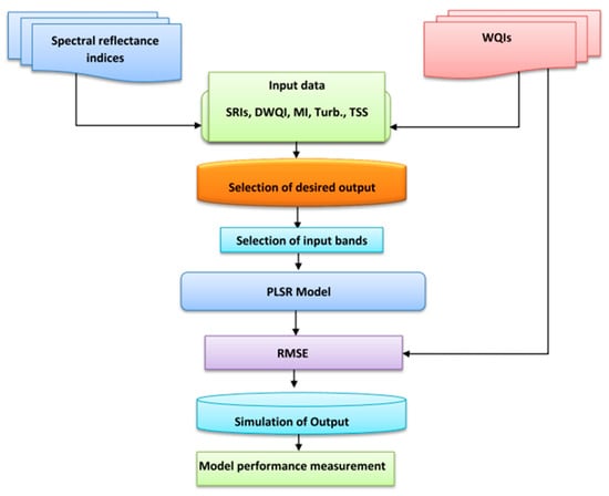
Figure 2.
Flowchart diagram of the methodology for estimating water quality indices (WQIs) using PLSR model.
2.7. Data Analysis
Multivariate statistical analyses were performed on the physical and chemical data utilizing SPSS software version 22 (SPSS Inc., Chicago, IL, USA) to generate summary statistics. Piper trilinear diagram [], Gibbs diagram [], Chadha diagram [], and hydrochemical facies evolution diagram (HFE) [] were applied using Geochemist’s Workbench Student Edition 12.0 software to determine surface water types, geochemical processes, geochemical influencing factors, and the categorization of surface water samples and their controlling mechanisms. Multivariate modeling techniques such as CA and PCA are commonly utilized for assessing water quality. Therefore, by minimizing the chemical analysis data into common patterns, the CA was used to identify the physicochemical characteristics based on their similarities []. The PCA was used to study the association between the physicochemical properties that were responsible for changes in water quality by converting the initial variables into a new set that reflected the effect of significant elements on water quality. PAST program (version 3.25) was used to interpret the chemical analysis data on the physicochemical concentrations for CA and PCA. Finally, the spatial distribution maps for the WQI values at 51 locations along the Nile River were created using GIS software version 10.
3. Results and Discussion
3.1. Physical and Chemical Parameters
The physicochemical characteristics of Nile River water have been widely investigated as helpful criteria for understanding the state of water geochemistry and related regulatory processes that play critical roles in the evolution of water quality. Table 4 and Figure 3 give statistical summaries of the physicochemical properties of the investigated surface water points (min., max., and mean).
Table 4.
Statistical analysis of the physical and chemical parameters of surface water samples from the Nile River.
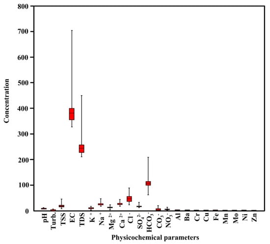
Figure 3.
Box plot of the physicochemical parameters of the investigated surface water points.
The obtained analytical values for the physical and chemical properties of surface water samples across the Nile River branches showed that temperature ranged from 27.0 °C to 33.7 °C with a mean value of 28.4 °C. Temperature influences the frequency of chemical processes and interaction between contaminants and aquatic inhabitants. The pH ranged from 7.40 to 8.40, with a mean of 7.85, indicating that the water samples were virtually normal to sub-alkaline in character []. Several water quality indicators, including Turb., and TSS, are critical in expressing surface water quality. Therefore, these measures are the primary indicator metrics for assessing surface water quality and its degradation as a result of polluting activities. Turbidity, a measure of the purity of water, varied from 0.23 NTU to 10.62 NTU with a mean of 3.33 NTU along the Nile River. In addition, the TSS values varied from 8.39 mg/L to 45.20 mg/L with a mean of 19.26 mg/L. Turbidity and TSS levels increased at several points along the watercourse as a result of the excessive drainage of various swept-out effluents into the Nile River. The occurrence of suspended particles including silt, clay, organic compounds, and plankton and other microorganisms generates Turb. in water [,]. Most of the urban activities that occur along the river contribute to increased Turb. The EC readings ranged from 328.0 to 703.0 μs/cm, with an average value of 393.06 μs/cm. In addition, the TDS levels varied from 210.0 mg/L to 450.0 mg/L, with a mean value of 251.53 mg/L, which reflected fresh water type. The ionic content of K+, Na2+, Mg2+, Ca2+, Cl−, SO42−, HCO32−, CO3− and NO3− showed mean values of 8.50, 25.06, 12.57, 26.07, 45.88, 16.02, 106.11, 5.22 and 5.74 mg/L, respectively (Table 5). Therefore, the average values of ions showed sequences of Ca2+ > Na2+ > Mg2+ > K+ and HCO32− > Cl− > SO42− > NO3− > CO3−, respectively. These results revealed that Ca2+ was the dominant cation and HCO32- was the dominant anion in the collected surface water samples.
Table 5.
Classification of the different water quality indices (WQIs).
The mean contents of Al, Ba, Cr, Cu, Fe, Mn, Mo, Ni, and Zn were 0.52, 0.045, 0.0046, 0.0046, 0.433, 0.047, 0.0092, 0.0183, and 0.0161 mg/L, respectively, and showed a sequence of Al > Fe > Mn > Ba > Ni > Zn > Mo > Cr > Cr (Table 4). To our understanding, metals in water derived from a variety of sources, such as rock–water interaction, weathering process, and human activities. The concentration of metals in the collected samples varied significantly throughout the river, which showed high levels of Al and Fe content above the specified acceptable limits for potable consumption [].
3.2. Geochemical Facies and Controlling Mechanisms
To better understand the geochemical mechanisms that govern water quality, hydrochemical data were analyzed through imitative approaches. Piper’s trilinear diagram was used to determine the prevalent cations and anions in meq/L of the investigated samples in order to define the geochemical facies and surface water types in the Nile River (Figure 4a). The chemical characteristics of the analyzed surface water samples showed Ca-HCO3 and mixed Ca-Mg-Cl-SO4 water types, which reflected meteoric water and initial stages of evolution []. Chadah’s categorization was also conducted to identify hydrochemical pathways and surface water types (Figure 4b). The surface water samples were dispersed in fields 1 and 3, which demonstrated recent recharge water associated with cation exchange processes in the surface water system, particularly in the downstream of the Nile River, that reflected an increase in Ca2+ concentration, thus indicating meteoric water type.
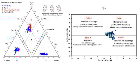
Figure 4.
Surface water type and geochemical processes in the Nile River: (a) Piper diagram and (b) Chadha diagram.
The relations between TDS vs. (Na + K)/(Na + K + Ca) and Cl/(Cl + HCO3) were applied using Gibb’s diagram to identify the geochemical regulating mechanisms influencing water quality. The surface water points were distributed in the evaporation field (Figure 5a), which was a significant process governing surface water quality. The hydrochemical facies evolution diagram (HFE) plot results revealed high contents of calcium and bicarbonate in surface water samples (Figure 5b).
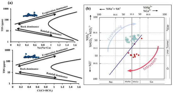
Figure 5.
Geochemical controlling mechanisms influencing water quality in the Nile River: (a) Gibbs diagram and (b) hydrochemical facies evolution diagram (HFE).
3.3. Water Quality Indices (WQIs)
The statistical descriptions of several WQIs and the categorization of water quality based on WQI references are presented in Table 5.
3.3.1. Drinking Water Quality Index (DWQI)
The DWQI model was applied to assess surface water quality and measure the acceptability of surface water for drinking, which was categorized depending on the purity level of measured physicochemical parameters according to Equation (1). The computed value of DWQI in the investigated samples ranged from 35.22 to 239.68, with an average of around 100.32. According to the DWQI categorization, about 53% of the surface water varied from excellent to good water for drinking purposes, while about 43% varied from poor to very poor water, and 4% of samples represented water unsuitable for drinking. According to the DWQI spatial distribution map, the degradation in water quality may be linked to a poor drainage system, discharges from huge tracts in agricultural regions, and industrial wastewater effluent along the Nile River (Figure 6a).
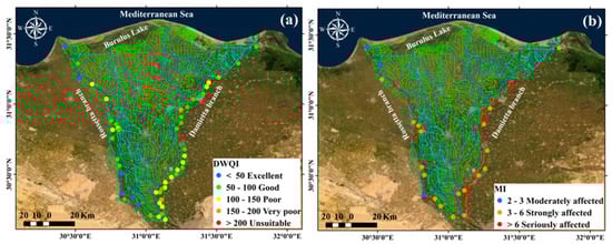
Figure 6.
Spatial distribution maps of water quality indices (WQIs) along the Nile River: (a) drinking water quality index (DWQI) and (b) metal index (MI).
3.3.2. Pollution Indices (PIs)
The PIs are regarded as an effective method to assess the appropriateness of water for drinking purposes with respect to metals []. The MI results for the collected water sampling points varied from 1.81 to 29.00, with a mean value of 8.48, which revealed that 59% of samples were seriously affected by metals, about 35% of samples were strongly affected, and only 6% of samples were moderately affected. According to the spatial variation map of MI values, surface water samples from the Damietta branch were more affected by metals than those from the Rosetta branch, especially in the dissected points with drainage (Figure 6b). According to the MI findings, water from the majority of sample collection points along the Nile River was not suitable for potable use and should be treated before drinking, particularly along the Damietta branch, as a result of poor drainage systems and human activities [,].
According to the categorization of PI levels, the PI values indicated that the water collection points were not affected by Ba, Cr, Cu, Mn, Mo, Ni and Zn (PI > 1.0), but moderately affected by Fe (PI = 4.01) and strongly affected by Al (PI = 9.43), as presented in Table 6.
Table 6.
Evaluation of surface water quality based on the effects of metals across the Nile River.
The high Fe loading may be related to soil–water interactions, whereas the high Al loading could be linked to industrial activity and poor sanitation infrastructure. Spatial distribution maps of PI values revealed the deterioration of surface water quality for drinking near areas of intensive human activities along the Rosetta and Damietta branches, which were influenced by metals, according to the integration between DWQI and MI. Therefore, surface water quality in the examined region is deteriorating as a result of rising levels of swept-out pollutants discharged into the Nile River from various drainage sources.
3.4. Multivariate Statistical Analysis for Physicochemical Parameters
By combining the independent dataset into a collection of variables, CA and PCA were applied to discover the sources of variations in water quality (Figure 6).
3.4.1. Cluster Analysis (CA)
The CA findings for the physicochemical parameters indicated three types of clustering (Figure 7a). For example, TDS was in a single cluster (Cluster 1), while HCO32 and Cl− were in another cluster (Cluster II), and K+, Ca2+, Mg2+, Na+, SO42−HCO32−, CO32− and NO3− were in different cluster (Cluster III). Based on the CA of major ions, surface water samples from the examined areas were classified by Ca2+ and Na+ as the dominant cations, while HCO32− and SO42− were the dominant anions (Figure 7a). Moreover, the high Ca2+\ content suggested water in the initial stage of evolution, which indicated the release of Ca2+ by weathering of carbonate minerals, while the high HCO32− and Cl− contents reflected meteoric water type. The CA results are in agreement with the results provided by the Piper diagram, which reflected the effects of carbonate weathering and reverse ion exchange processes that were also reported in the Gibbs and Chadha diagrams.
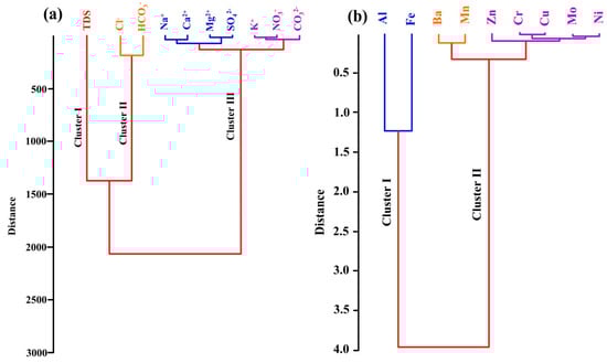
Figure 7.
Cluster analysis for physicochemical parameters along the Nile River: (a) CA for major ions and (b) CA for metals.
The CA results for trace elements and metals indicated two types of clustering (Figure 7b), with Al and Fe included in the same cluster (Cluster I), and Ba, Cr, Cu, Mn, Mo, Ni and Zn in another cluster (Cluster II). Accordingly, the high contents of Al and Fe reflected water–soil interaction and human activities.
3.4.2. Principal Component Analysis (PCA)
PCA findings for the physicochemical properties of the main ions in the obtained surface water samples are shown in Figure 8a. According to positive loading combinations, all cations and anions were grouped together. Large positive loadings of TDS, Ca2+, K+, SO42−, HCO32−, and CO32− prevailed over PC1 in explaining 40.761% of total variance, while, PC1 explained 17.847% of total variance, in which loadings of Na+, Mg2+, Cl−, and NO3− prevailed (Figure 8a). The existence of nine important basic principal components in the PCA analyses revealed the effect of significant ions on water quality in the investigated regions. Therefore, PC1 presented maximum loadings of Ca2+ and HCO32−, while PC2 presented maximum loadings of Na+ and Cl−. These findings could be attributing to carbonate weathering, evaporation and reverse ion exchange processes.
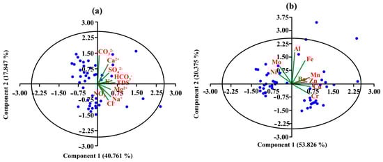
Figure 8.
Principal component analysis of physicochemical parameters along the Nile River: (a) PCA of major ions and (b) PCA of trace elements and metals.
The PCA was performed for metals in the collected surface water samples and explained 53.826% (PC1) and 20.375% (PC2) of the total variation between metals (Figure 8b). Therefore, PC1 presented high loadings of Al, Fe, Ba, Cr, Cu, Mn, and Zn, while PC2 presented high loadings of Mo, and Ni as a result of the effect of metals on surface water quality (Figure 8b). The PCA analysis of surface water samples for major ions and metals revealed lithogenic sources and human activities, respectively. As a consequence, due to the high loadings of Al, Fe, Ba, Cr, Cu, Mn, and Zn, these findings may be related to soil–water interaction and industrial and other anthropogenic practices [,,]. There was high agreement between PCA and MI, indicating that most of the surface water points in the research region had bad water attributable to metal pollution. Therefore, the PCA and PI results reflected the lithogenic and economic sources of pollution that have emerged in recent years along the Rosetta and Damietta branches.
3.5. Performance of Different SRIs in the Assessment of Water Quality Indicators
Several studies have explored the effectiveness of space-based optical remote sensing devices for water quality assessment. While the majority only looked at physiochemical and biological water quality metrics such as Turb., chlorophyll-a and TSS and dissolved organic matter concentrations [,,,,,,], they provided little information about using proximate hyperspectral sensing to estimate the DWQI and MI of surface water. The newly derived SRIs were developed using 2-D correlogram maps constructed from spectral reflectance of two Nile River branches. The values of the coefficient of determination (R2) for the associations between records of DWQI, MI, Turb., and TSS and SRIs produced from all conceivable combinations of binary dual wavelengths in the whole spectral range (302–1148 nm) were displayed on these maps (Figure 9). The greatest R2 hotspot area revealed the best relationships between SRIs and water quality indices. The selected SRIs in Table 3 were established using spectral data of water quality indicators in the VIS at several bands (VIS range: 470, 490, 514,540, 530, 560, 570, 580, 584, 590, 608, 620, 628, 640, 670, 686, and 698 nm) and in the NIR range (700, 704, 717, 720, 730, 760, 776,780, and 850 nm).
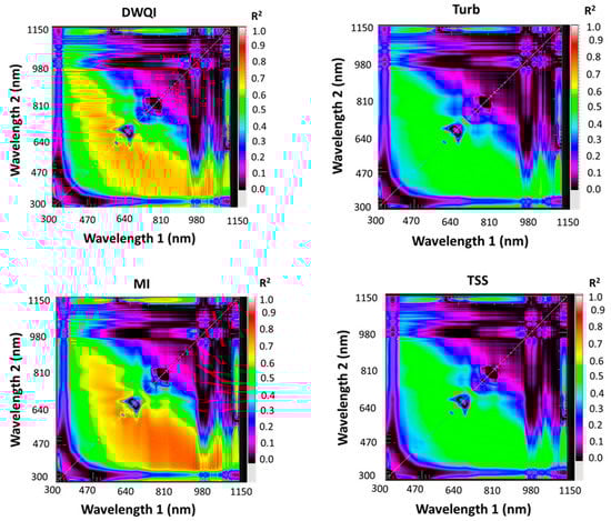
Figure 9.
Correlation matrices show R2 values for the spectra’s potential dull wavelength combinations in the spectrum from 302 to 1148 nm with drinking water quality index (DWQI), metal index (MI), turbidity (Turb.) and total suspended solids (TSS). R2 values were calculated across all pooled data (n = 51).
This finding emphasizes the relevance of the VIS and NIR spectrum wavelength ranges in evaluating WQIs of the Nile River. In line with expectations, the qualities of the emissions reflected from the water components in distinct bands of the light spectrum were affected by differences in the physical and chemical constituents of water utilized to analyze and manage the quality of surface water. Several studies discovered that the VIS, red-edge, and NIR regions of the light spectrum have greater correlations with distinct physicochemical water components in different water bodies than other spectral regions, implying that these spectral regions might be utilized to measure water quality characteristics [,,,,,,,].
Table 7 shows the relationships of DWQI, MI, Turb., and TSS with the SRIs of the water samples from Nile River branches. In general, all published and newly derived indices showed the same pattern of relationships with all WQIs for each Nile River branch and their combinations. All indices exhibited significant relationships with these indices. The newly derived SRIs presented higher R2 with DWQI, MI, Turb., and TSS compared with published indices. The new SRIs extracted from the VIS and NIR regions exhibited strong relationships with DWQI and MI and moderate to strong relationships with Turb. and TSS for each branch of the Nile River and their combination. The R2 for relationships between the newly derived SRIs and WQIs varied from 0.65 to 0.82 for DWQI, from 0.64 to 0.83 for MI, from 0.41 to 0.60 for Turb., and from 0.35 to 0.79 for TSS. The R2 for relationships between the published SRIs and QWIs varied from 0.41 to 0.80 for DWQI, from 0.41 to 0.85 for MI, from 0.19 to 0.74 for Turb., and from 0.29 to 0.79 for TSS. With data from the samples collected along the two branches combined, the SRI extracted from red, red-edge and green regions showed the highest R2 for WQIs. For example, the published index of green/red presented the highest values of R2 = 0.70, 54, and 0.54 for DWQI, Turb., and TSS, respectively, as well as RSI670,470 presented R2 = 0.73 for MI. The new index of RSI584,628 presented the highest values of R2 = 0.72, 0.57, and 0.57 for DWQI, Turb., and TSS, respectively, as well as RSI730,540 presented R2 = 0.73 for MI. Other studies such as Seyhan et al. [] found that in the range of 400–900 nm, the spectral signatures were favorable for water quality assessment. Additionally, Elhag et al. [] found that water Turb. measurements revealed a strong relationship with the calculated normalized difference in the Turb. index, with an R2 of 0.94. In addition, Wang et al. [] found that DWQI could be easily assessed at 700–720 nm and 1070 nm of the peak. They also discovered that spectral curves for various water samples revealed numerous prominent, deep absorption regions at 700, 750, 950, and 980 nm and weak absorption regions at 452, 703, and 850 nm.
Table 7.
R2 for the linear association between SRIs and drinking water quality index (DWQI), metal index (MI), turbidity (Turb.) and total suspended solids (TSS). Estimates were calculated for Rosetta branch (n = 21), Damietta branch (n = 30) and across all data (n = 51).
3.6. Prediction of Different WQIs Using PLSR Models
Despite the fact that SRIs are a simple method of WQI evaluation that may be used to construct ground-based lightweight spectral instruments for estimating and regulating water quality on a broad scale in a timely and economical manner, each SRI is only concerned with two or three band combinations. This makes developing effective SRIs difficult for estimating WQIs under a variety of potentially confusing variables, such as considerable variations in water component quantities, as well as their impact on the saturation level of the water quality measurements under investigation. For that reason, in this study, the PLSR model was applied to estimate water quality indicators including several SRIs as input variables.
Table 8 summarizes the determination coefficient (R2) values and the RMSE of the PLSR models’ calibration (Cal.) and validation (Val.) datasets to predict DWQI, MI, Turb. and TSS based on SRIs in Table 4. The performance of the PLSR calibration models in predicting the four surface indicators was based on pooled data across the two branches of the Nile River (n = 51). Following that, the calibration equations of the models were applied to predict DWQI, MI, Turb. and TSS of the Rosetta branch (n = 21) and Damietta branch (n = 30). In both models of the Cal. and Val. datasets, the PLSR model produced a more accurate assessment of DWQI and MI based on values of R2 (Table 8) and slope (Figure 10) than of other factors such as Turb. and TSS. In Val. datasets, the PLSR model generated strong estimates for the DWQI and MI with R2 of 0.82 and 0.79 and RMSE of 20.82 and 2.77, respectively, for the Rosetta branch and with R2 of 0.93 and 0.78 and RMSE of 11.67 and 2.22, respectively, for the Damietta branch. However the PLSR model provided moderate estimation performance for Turb. and TSS in the Val. datasets, with R2 of 0.55 and 0.62 and RMSE of 1.18 and 6.60, respectively, for the Rosetta branch and with R2 of 0.62 and 0.70 and RMSE of 0.89 and 4.04, respectively, for the Damietta branch. The results showed that the PLSR based on several SRIs could be used to predict WQIs better than using two bands. Wang et al. [] discovered that detecting TSS in moderately clear water using a single band or two waveband combinations is difficult. However, in turbid water bodies, a combination of three wavebands proved successful in estimating Chl-a levels [,]. Wang et al. [] discovered that PLSR models with a large number of wavebands were more precise in predicting inland water quality indicators than models with only one or two wavebands. Once again, PLSR models built on different SRIs can be utilized as a unified approach for remote measurement of WQIs in water quality evaluations.
Table 8.
Calibration and validation models between the observed and predicted values (R2 and RMSE) based on PLSR. These models were calibrated using a dataset for two Nile River branches. Following that, the calibration equations for various models were used to predict drinking water quality index (DWQI), metal index (MI), turbidity (Turb.) and total suspended solids (TSS) for each branch.
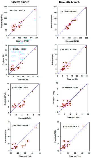
Figure 10.
Association between observed and predicted validation models for drinking water quality index (DWQI), metal index (MI), turbidity (Turb.) and total suspended solids (TSS) for each river branch using the PLSR based on selected SRIs. Statistical analysis including R2, p-value and RMSE is shown in Table 8.
4. Conclusions
This research proposed comprehensive methodologies supported by SRIs, CA, PCA, and PLSR for assessing, in terms of physicochemical properties, the acceptability of surface water quality for drinking. Under the stresses of evaporation and the reverse ion exchange processes, surface water samples in the examined region were classified as Ca-HCO3 and mixed Ca-Mg-Cl-SO4 water types, which were seriously affected by Al and moderately affected by Fe due to soil–water interactions and industrial activities. According to the WQI results, the degradation in water quality may be linked to poor drainage systems, discharges from huge tracts of agricultural regions, industrial wastewater emissions, and a poor sanitation infrastructure along the Nile River. With combined data from two surface water branches, the SRI extracted from red, red-edge and green regions showed the highest R2 with four indices. For example, the published index of green/red presented the highest R2 = 0.70, 54, 0.54 for DWQI, Turb. and TSS, respectively, as well as RSI670,470 presented R2 = 0.73 for MI. The newly derived index of RSI584,628 presented the highest R2 = 0.72, 0.57and 0.57 for DWQI, Turb. and TSS, respectively, as well as RSI730,540 presented R2 = 0.73 for MI. PLSR models based on several SRIs could enhance the estimation of numerous WQIs and could be employed as a unified approach for remote component concentration measurements in water quality assessments. Therefore, the integration of WQIs, SRIs, multivariate modeling, and GIS techniques is beneficial and can provide us with a comprehensive image of surface water suitability for drinking and its governing mechanisms.
Author Contributions
Conceptualization, M.G. and S.E.; Methodology, M.G., A.H.S., H.H., M.F. and S.E.; Software, M.G., S.E., M.F., A.H.S. and H.H.; Formal Analysis, M.G., S.E., H.H.; M.F. and A.H.S.; Resources, M.G.; Data Curation, M.G., S.E. and A.H.S. Writing—Original Draft Preparation, M.G., S.E., H.H., M.F. and A.H.S.; Writing—Review and Editing, M.G. and S.E.; Supervision, M.G. and S.E.; Project Administration, M.G.; Funding Acquisition, M.G. All authors have read and agreed to the published version of the manuscript.
Funding
The paper is based upon work supported by University of Sadat City (USC) under grant No. (17).
Institutional Review Board Statement
Not applicable.
Informed Consent Statement
Not applicable.
Data Availability Statement
Data are contained within the article.
Acknowledgments
The authors extend their appreciation to the University of Sadat City (USC), Egypt, for funding this research work through the project number (17).
Conflicts of Interest
The authors declare no conflict of interest.
References
- Higler, L.W.G. Fresh Surface Water: Biology and Biodiversity of River Systems. In Encyclopedia of Life Support Systems (EOLSS); ALTERRA: Wageningen, The Netherlands, 2012. [Google Scholar]
- Loucks, D.P.; van Beek, E. Water quality modeling and prediction. In Water Resource Systems Planning and Management: An Introduction to Methods, Models, and Applications; Springer International Publishing: Cham, Switzerland, 2017; pp. 417–467. [Google Scholar]
- Gupta, S.; Gupta, S.K. A critical review on water quality index tool: Genesis, evolution and future directions. Ecol. Inform. 2021, 63, 101299. [Google Scholar] [CrossRef]
- Devi, P.; Singh, P.; Kansal, S.K. Inorganic Pollutants in Water; Elsevier: Amsterdam, The Netherlands, 2020. [Google Scholar]
- Kareem, S.L.; Mohammed, A.A. Removal of tetracycline from wastewater using circulating fluidized bed. Iraqi J. Chem. Pet. Eng. 2020, 21, 29–37. [Google Scholar] [CrossRef]
- Kareemb, S.L.; Jaberc, W.S.; Al-Malikia, L.A.; Al-husseinyb, R.A.; Al-Mamooria, S.K.; Alansarid, N. Water quality assessment and phosphorus effect using water quality indices: Euphrates River-Iraq as a case study. Groundw. Sustain. Dev. 2021, 14, 100630. [Google Scholar] [CrossRef]
- Elhaddad, E.; Al-Zyoud, S. The quality assessment of pollution of Rosetta branch, Nile River, Egypt. Arab. J. Geosci. 2017, 10, 97. [Google Scholar] [CrossRef]
- Duda, R.; Klebert, I.; Zdechlik, R. Groundwater pollution risk assessment based on vulnerability to pollution and potential impact of land use forms. Pol. J. Environ. Stud. 2020, 29, 87–99. [Google Scholar] [CrossRef]
- Khazheeva, Z.I.; Plyusnin, A.M.; Smirnova, O.K.; Peryazeva, E.G.; Zhambalova, D.I.; Doroshkevich, S.G.; Dabaeva, V.V. Mining activities and the chemical composition of R. Modonkul, Transbaikalia. Water 2020, 12, 979. [Google Scholar] [CrossRef]
- Tomaszewska, B.; Bundschuh, J.; Pająk, L.; Dendys, M.; Quezada, V.D.; Bodzek, M.; Armienta, M.A.; Muñoz, M.O.; Kasztelewicz, A. Use of low-enthalpy and waste geothermal energy sources to solve arsenic problems in freshwater production in selected regions of Latin America using a process membrane distillation—Research into model solutions. Sci. Total Environ. 2020, 714, 136853. [Google Scholar] [CrossRef]
- Elsayed, S.; Hussein, H.; Moghanm, F.S.; Khedher, K.M.; Eid, E.M.; Gad, M. Application of irrigation water quality indices and multivariate statistical techniques for surface water quality assessments in the Northern Nile Delta, Egypt. Water 2020, 12, 3300. [Google Scholar] [CrossRef]
- El Bouraie, M.M.; El Barbary, A.A.; Yehia, M.M.; Motawea, E.A. Heavy metal concentrations in surface river water and bed sediments at Nile Delta in Egypt. Suoseura 2010, 61, 1–12. [Google Scholar]
- Abdel-Satar, A.M.; Ali, M.H.; Goher, M.E. Indices of water quality and metal pollution of Nile River, Egypt. Egypt. J. Aquat. Res. 2017, 43, 21–29. [Google Scholar] [CrossRef]
- El Sayed, S.M.; Hegab, M.H.; Mola, H.R.A.; Ahmed, N.M.; Goher, M.E. An integrated water quality assessment of Damietta and Rosetta branches (Nile River, Egypt) using chemical and biological indices. Environ. Monit. Assess. 2020, 192, 228. [Google Scholar] [CrossRef] [PubMed]
- Taher, M.E.; Ghoneium, A.M.; Hopcroft, R.R.; ElTohamy, W.S. Temporal and spatial variations of surface water quality in the Nile River of Damietta Region, Egypt. Environ. Monit. Assess. 2021, 193, 128. [Google Scholar] [CrossRef] [PubMed]
- Gad, M.; Abou El-Safa, M.M.; Farouk, M.; Hussein, H.; Alnemari, A.M.; Elsayed, S.; Khalifa, M.M.; Moghanm, F.S.; Eid, E.M.; Saleh, A.H. Integration of Water Quality Indices and Multivariate Modeling for Assessing Surface Water Quality in Qaroun Lake, Egypt. Water 2021, 13, 2258. [Google Scholar] [CrossRef]
- Zhang, X.; Hu, B.X.; Wang, P.; Chen, J.; Yang, L.; Xiao, K. Hydrogeochemical evolution and heavy metal contamination in groundwater of a reclaimed land on Zhoushan Island. Water 2018, 10, 316. [Google Scholar] [CrossRef]
- Gad, M.; El-Hattab, M. Integration of water pollution indices and DRASTIC model for assessment of groundwater quality 640 in El Fayoum Depression, Western Desert, Egypt. J. Afr. Earth Sci. 2019, 158, 103554. [Google Scholar] [CrossRef]
- Gad, M.; El Osta, M. Geochemical controlling mechanisms and quality of the groundwater resources in El Fayoum Depression, Egypt. Arab. J. Geosci. 2020, 13, 861. [Google Scholar] [CrossRef]
- Semiromi, F.B.; Hassani, A.; Torabian, A.; Karbassi, A.; Lotfi, F.H. Water quality index development using fuzzy logic: A case study of the Karoon River of Iran. Afr. J. Biotechnol. 2011, 10, 10125–10133. [Google Scholar]
- Vinod, J.; Satish, D.; Sapana, G. Assessment of water quality index of industrial area surface water samples. Int. J. ChemTech Res. 2013, 5, 278–283. [Google Scholar]
- Guo, Q.; Wang, Y. Impact of geothermal wastewater drainage on arsenic species in environmental media: A case study at the Yangbajing geothermal field, Tibet, China. Procedia Earth Planet. Sci. 2013, 7, 317–320. [Google Scholar] [CrossRef][Green Version]
- Gitau, M.W.; Chen, J.; Ma, Z. Water quality indices as tools for decision making and management. Water Resour. Manag. 2016, 30, 2591–2610. [Google Scholar] [CrossRef]
- Mukate, S.; Wagh, V.; Panaskar, D.; Jacobs, J.A.; Sawant, A. Development of new integrated water quality index (IWQI) model to evaluate the drinking suitability of water. Ecol. Indic. 2019, 101, 348–354. [Google Scholar] [CrossRef]
- Wątor, K.; Zdechlik, R. Application of water quality indices to the assessment of the effect of geothermal water discharge on river water quality—Case study from the Podhale region (Southern Poland). Ecol. Indic. 2021, 121, 107098. [Google Scholar] [CrossRef]
- Bhargava, D.; Saxena, B.; Dewakar, A. A Study of Geopollutants in the Godavary River Basin in India, Asian Environment; IOS Press: Amsterdam, The Netherlands, 1998. [Google Scholar]
- Dwivedi, S.; Tiwari, I.; Bhargava, D. Water Quality of the River Ganga at Varanasi. J. Inst. Eng. India Part E Environ. Eng. Div. 1997, 78, 1–4. [Google Scholar]
- Noori, R.; Berndtsson, R.; Hosseinzadeh, M.; Adamowski, J.F.; Abyaneh, M.R. A critical review on the application of the national sanitation foundation water quality index. Environ. Pollut. 2019, 244, 575–587. [Google Scholar] [CrossRef]
- Kim, J.H.; Kim, R.H.; Lee, J.; Cheong, T.J.; Yum, B.W.; Chang, H.W. Multivariate statistical analysis to identify the major factors governing groundwater quality in the coastal area of Kimje, South Korea. Hydrol. Process. Int. J. 2005, 19, 1261–1276. [Google Scholar] [CrossRef]
- Noori, R.; Sabahi, M.S.; Karbassi, A.R.; Baghvand, A.; Zadeh, H.T. Multivariate statistical analysis of surface water quality based on correlations and variations in the data set. Desalination 2010, 260, 129–136. [Google Scholar] [CrossRef]
- Hamid, A.; Bhat, S.A.; Bhat, S.U.; Jehangir, A. Environmetric techniques in water quality assessment and monitoring: A case study. Environ. Earth Sci. 2016, 75, 321. [Google Scholar] [CrossRef]
- Jung, K.Y.; Lee, K.L.; Im, T.H.; Lee, I.J.; Kim, S.; Han, K.Y.; Ahn, J.M. Evaluation of water quality for the Nakdong River watershed using multivariate analysis. Environ. Technol. Innov. 2016, 5, 67–82. [Google Scholar] [CrossRef]
- Barzegar, R.; Moghaddam, A.A.; Tziritis, E.; Adamowski, J.; Nassar, J.B.; Noori, M.; Kazemian, N. Exploring the hydrogeochemical evolution of cold and thermal waters in the Sarein-Nir area, Iran using stable isotopes (δ18O and δD), geothermometry and multivariate statistical approaches. Geothermics 2020, 85, 101815. [Google Scholar] [CrossRef]
- El Osta, M.; Masoud, M.; Alqarawy, A.; Elsayed, S.; Gad, M. Groundwater Suitability for Drinking and Irrigation Using Water Quality Indices and Multivariate Modeling in Makkah Al-Mukarramah Province, Saudi Arabia. Water 2022, 14, 483. [Google Scholar] [CrossRef]
- Tariq, R.S.; Shah, M.H.; Shaheen, N.; Khalique, A.; Manzoor, S.; Jaffar, M. Multivariate analysis of selected metals in tannery effluents and related soil. J. Hazard. Mater. 2005, A122, 17–22. [Google Scholar] [CrossRef] [PubMed]
- Tariq, S.R.; Shaheen, N.; Khalique, A.; Sha, M.H. Distribution, correlation, and source apportionment of selected metals in tannery effluents, related soils, and groundwater—A case studies from Multan, Pakistan. Environ. Monit. Assess. 2010, 166, 303–312. [Google Scholar] [CrossRef] [PubMed]
- Chidambaram, S.; Karmegam, U.; Prasanna, M.V.; Sasidhar, P. A study on evaluation of probable sources of heavy metal pollution in groundwater of Kalpakkam region, South India. Environmentalist 2012, 32, 371–382. [Google Scholar] [CrossRef]
- Prasanna, M.V.; Praveena, S.M.; Chidambaram, S.; Nagarajan, R.; Elayaraja, A. Evaluation of water quality pollution for heavy metal contamination monitoring: A case study from Curtin Lake. Environ. Earth Sci. 2012, 67, 1987–2001. [Google Scholar] [CrossRef]
- Sharma, G.; Lata, R.; Thakur, N.; Bajala, V.; Kuniyal, J.C.; Kumar, K. Application of multivariate statistical analysis and water quality index for quality characterization of Parbati River, Northwestern Himalaya, India. Discov. Water 2021, 1, 5. [Google Scholar] [CrossRef]
- Franco-Uria, A.; Lopez-Mateo, C.; Roca, E.; Eernandez-Marcos, M.L. Source identification of heavy metals in pastureland by multivariate analysis in NW Spain. J. Hazard. Mater. 2009, 165, 1008–1015. [Google Scholar] [CrossRef] [PubMed]
- Kwaya, M.Y.; Hamidu, H.; Kachalla, M.; Abdullahi, I.M. Preliminary Ground and Surface Water Resources Trace Elements Concentration, Toxicity and Statistical Evaluation in Part of Yobe State, North Eastern Nigeria. Geosciences 2017, 7, 117–128. [Google Scholar]
- De Bartolomeo, A.; Poletti, L.; Sanchini, G.; Sebastiani, B.; Morozzi, G. Relationship among parameters of lake polluted sediments evaluated by multivariate statistical analysis. Chemosphere 2004, 55, 1323–1329. [Google Scholar] [CrossRef]
- Kalamaras, N.; Michalopoulou, H.; Byun, H.R. Detection of drought events in Greece using daily precipitation. Hydrol. Res. 2010, 41, 126–133. [Google Scholar] [CrossRef]
- Wang, M.; Markert, B.; Chen, W.; Peng, C.; Ouyang, Z. Identification of heavy metal pollutants using multivariate analysis and effects of land uses on their accumulation in urban soils in Beijing, China. Environ. Monit. Assess. 2012, 184, 5889–5897. [Google Scholar] [CrossRef]
- Ahmad, T.; Gupta, G.; Sharma, A.; Kaur, B.; Alsahli, A.A.; Ahmad, P. Multivariate Statistical Approach to Study Spatiotemporal Variations in Water Quality of aHimalayan Urban Fresh Water Lake. Water 2020, 12, 2365. [Google Scholar] [CrossRef]
- Gitelson, A.; Garbuzov, G.; Szilagyi, F.; Mittenzwey, K.H.; Karnieli, A.; Kaiser, A. Quantitative remote-sensing methods for real-time monitoring of inland waters quality. Int. J. Remote Sens. 1993, 14, 1269–1295. [Google Scholar] [CrossRef]
- Xing, Z.; Chen, J.; Zhao, X.; Li, Y.; Li, X.; Zhang, Z.; Lao, C.; Wang, H. Quantitative estimation of wastewater quality parameters by hyperspectral band screening using GC, VIP and SPA. PeerJ 2019, 7, e8255. [Google Scholar] [CrossRef] [PubMed]
- Wei, L.; Huang, C.; Zhong, Y.; Wang, Z.; Hu, X.; Lin, L. Inland waters suspended solids concentration retrieval based on PSO-LSSVM for UAV-borne hyperspectral remote sensing imagery. Remote Sens. 2019, 11, 1455. [Google Scholar] [CrossRef]
- Gholizadeh, M.H.; Melesse, A.M.; Reddi, L.A. A Comprehensive review on water quality parameters estimation using remote sensing techniques. Sensors 2016, 16, 1298. [Google Scholar] [CrossRef]
- Song, K.; Li, L.; Li, S.; Tedesco, L.; Hall, B.; Li, L. Hyperspectral remote sensing of total phosphorus (TP) in three central Indiana water supply reservoirs. Water Air Soil Pollut. 2012, 223, 1481–1502. [Google Scholar] [CrossRef]
- Giardino, C.; Bresciani, M.; Cazzaniga, I.; Schenk, K.; Rieger, P.; Braga, F.; Matta, E.; Brando, V.E. Evaluation of multi-resolution satellite sensors for assessing water quality and bottom depth of Lake Garda. Sensors 2014, 14, 24116–24131. [Google Scholar] [CrossRef] [PubMed]
- Khadr, M.; Gad, M.; El-Hendawy, S.; Al-Suhaibani, N.; Dewir, Y.H.; Tahir, M.U.; Mubushar, M.; Elsayed, S. The integration of multivariate statistical approaches, hyperspectral reflectance, and data-driven modeling for assessing the quality and suitability of groundwater for Irrigation. Water 2021, 13, 35. [Google Scholar] [CrossRef]
- Brando, V.E.; Braga, F.; Zaggia, L.; Giardino, C.; Bresciani, M.; Matta, E.; Bellafiore, D.; Ferrarin, C.; Maicu, F.; Benetazzo, A.; et al. High-resolution satellite turbidity and sea surface temperature observations of river plume interactions during a significant flood event. Ocean Sci. 2015, 11, 909–920. [Google Scholar] [CrossRef]
- Shareef, M.A.; Khenchaf, A.; Toumi, A. Integration of passive and active microwave remote sensing to estimate water quality parameters. In Proceedings of the Radar Conference, Philadelphia, PA, USA, 2–6 May 2016; pp. 1–4. [Google Scholar]
- Xiao, R.; Wang, G.; Zhang, Q.; Zhang, Z. Multi-scale analysis of relationship between landscape pattern and urban river water quality in different seasons. Sci. Rep. 2016, 6, 25250. [Google Scholar] [CrossRef]
- Yang, Y.; Gao, B.; Hao, H.; Zhou, H.; Lu, J. Nitrogen and phosphorus in sediments in china: A national-scale assessment and review. Sci. Total Environ. 2017, 576, 840–849. [Google Scholar] [CrossRef] [PubMed]
- Elhag, M.; Gitas, I.; Othman, A.; Bahrawi, J.; Gikas, P. Assessment of water quality parameters using temporal remote sensing spectral reflectance in arid environments, Saudi Arabia. Water 2019, 11, 556. [Google Scholar] [CrossRef]
- Elsayed, S.; Ibrahim, H.; Hussein, H.; Elsherbiny, O.; Elmetwalli, A.H.; Moghanm, F.S.; Ghoneim, A.M.; Danish, S.; Datta, R.; Gad, M. Assessment of water quality in Lake Qaroun using ground-based remote sensing data and artificial neural networks. Water 2021, 13, 3094. [Google Scholar] [CrossRef]
- Garriga, M.; Romero-Bravo, S.; Estrada, F.; Escobar, A.; Matus, I.A.; del Pozo, A.; Astudillo, C.A.; Lobos, G.A. Assessing wheat traits by spectral reflectance: Do we really need to focus on predicted trait-values or directly identify the elite genotypes group? Front. Plant Sci. 2017, 8, 280. [Google Scholar] [CrossRef]
- Gad, M.; El-Hendawy, S.; Al-Suhaibani, N.; Tahir, M.U.; Mubushar, M.; Elsayed, S. Combining hydrogeochemical characterization and a hyperspectral reflectance tool for assessing quality and suitability of two groundwater resources for irrigation in Egypt. Water 2020, 12, 2169. [Google Scholar] [CrossRef]
- Ezzet, S.M.; Mahdy, H.M.; Abo-State, M.A.; El Shakour, E.H.A.; El-Bahnasawy, M.A. Water quality assessment of Nile River at Rosetta branch: Impact of drains discharge. Middle East J. Sci. Res. 2012, 12, 413–423. [Google Scholar]
- Eltohamy, W.S.; Abdel-Baki, S.N.; Abdel-Aziz, N.E.; Khidr, A.A. Evaluation of spatial and temporal variations of surface water quality in the Nile River Damietta branch. Ecol. Chem. Eng. S 2018, 25, 569–580. [Google Scholar]
- APHA. Standard Methods for the Examination of Water and Wastewater; American Public Health Association: Washington, DC, USA, 2012. [Google Scholar]
- Ayandiran, T.A.; Fawole, O.O.; Dahunsi, S.O. Water quality assessment of bitumen polluted Oluwa River, South-Western Nigeria. Water Resour. Ind. 2018, 19, 13–24. [Google Scholar] [CrossRef]
- Kachroud, M.; Trolard, F.; Kefi, M.; Jebari, S.; Bourrie, G. Water quality indices: Challenges and application limits in the literature. Water 2019, 11, 361. [Google Scholar] [CrossRef]
- Lone, S.A.; Bhat, S.U.; Hamid, A.; Bhat, F.A.; Kumar, A. Quality assessment of springs for drinking water in the Himalaya of South Kashmir, India. Environ. Sci. Pollut. Control Ser. 2021, 28, 2279–2300. [Google Scholar] [CrossRef]
- Rawat, H.; Singh, R.; Namtak, S.; Deep, A.; Mamgain, S.; Sharma, A.; Kumar, R. Water quality assessment of Garhwal Himalayan Lake Tarakund based on the application of WQI and mitigation measures for its conservation and management. Int. J. Energy Water Resour. 2021, 5, 73–84. [Google Scholar] [CrossRef]
- Brown, R.M.; McCleiland, N.J.; Deininger, R.A.; O’Connor, M.F. A Water Quality Index—Crossing the Psychological Barrier. Proc. Int. Conf. Water Poll. Res. 1972, 6, 787–797. [Google Scholar]
- WHO. Guidelines for Drinking-Water Quality, 4th ed.; Incorporating the 1st Addendum; WHO: Geneva, Switzerland, 2017. [Google Scholar]
- Tamasi, G.; Cini, R. Heavy metals in drinking waters from Mount Amiata (Tuscany, Italy) possible risks from arsenic for public health in the province of Siena. Sci. Total Environ. 2004, 327, 41–51. [Google Scholar] [CrossRef] [PubMed]
- Ojekunle, O.Z.; Ojekunle, O.V.; Adeyemi, A.A.; Taiwo, A.G.; Sangowusi, O.R.; Taiwo, A.M.; Adekitan, A.A. Evaluation of surface water quality indices and ecological risk assessment for heavy metals in scrap yard neighbourhood. SpringerPlus 2016, 5, 2–16. [Google Scholar] [CrossRef]
- Caerio, S.; Costa, M.H.; Ramos, T.B.; Fernandes, F.; Silveira, N.; Coimbra, A.; Painho, M. Assessing heavy metal contamination in Sado Estuary sediment: An index analysis approach. Ecol. Indic. 2005, 5, 155–169. [Google Scholar] [CrossRef]
- Goher, M.E.; Mahdy, E.M.; Abdo, M.H.; El Dars, F.M.; Korium, M.A.; Elsherif, A.S. Water quality status and pollution indices of Wadi El-Rayan lakes, El-Fayoum, Egypt. Sustain. Water Resour. Manag. 2019, 5, 387–400. [Google Scholar]
- Chipman, J.W.; Olmanson, L.G.; Gitelson, A.A. Remote Sensing Methods for Lake Management: A Guide for Resource Managers and Decision-Makers; North American Lake Management Society: Madison, WI, USA, 2009. [Google Scholar]
- Somvanshi, S.; Kunwar, P.; Singh, N.; Shukla, S.; Pathak, V. Integrated remote sensing and GIS approach for water quality analysis of gomti river, Uttar Pradesh. Int. J. Environ. Sci. 2012, 3, 62–74. [Google Scholar]
- Bhatti, A.M.; Nasu, S.; Takagi, M.; Nojiri, Y. Assessing the potential of remotely sensed data for water quality monitoring of coastal and inland waters. Res. Bull. Kochi Univ. Technol. 2008, 5, 201–207. [Google Scholar]
- Wang, Z.; Kawamura, K.; Sakuno, Y.; Fan, X.; Gong, Z.; Lim, J. Retrieval of chlorophyll-a and total suspended solids using iterative stepwise elimination partial least squares (ISE-PLS) regression based on field hyperspectral measurements in irrigation ponds in Higashihiroshima, Japan. Remote Sens. 2017, 9, 264. [Google Scholar] [CrossRef]
- Shafique, N.A.; Autrey, B.C.; Fulk, F.; Cormier, S.M. Hyperspectral narrow wavebands selection for optimizing water quality monitoring on the Great Miami River, Ohio. J. Spat. Hydrol. 2001, 1, 1–22. [Google Scholar]
- Elsayed, S.; Gad, M.; Farouk, M.; Saleh, A.H.; Hussein, H.; Elmetwalli, A.H.; Elsherbiny, O.; Moghanm, F.S.; Moustapha, M.E.; Taher, M.A.; et al. Using Optimized Two and Three-Band Spectral Indices and Multivariate Models to Assess Some Water Quality Indicators of Qaroun Lake in Egypt. Sustainability 2021, 13, 10408. [Google Scholar] [CrossRef]
- Vinciková, H.; Hanuš, J.; Pechar, L. Spectral reflectance is a reliable water-quality estimator for small, highly turbid wetlands. Wetl. Ecol. Manag. 2015, 23, 933–946. [Google Scholar] [CrossRef]
- Menken, K.D.; Brezonik, P.L.; Bauer, M.E. Influence of chlorophyll and colored dissolved organic matter (CDOM) on Lake Reflectance Spectra: Implications for Measuring Lake Properties by Remote Sensing. Lake Reserv. Manag. 2006, 22, 179–190. [Google Scholar] [CrossRef]
- Wold, S.; Sjöström, M.; Eriksson, L. PLS-regression: A basic tool of chemometrics. Chemom. Intell. Lab. Syst. 2001, 58, 109–130. [Google Scholar] [CrossRef]
- Piper, A.M. A graphic procedure in the geochemical interpretation of water-analyses. EOS Trans. Am. Geophys. Union 1944, 25, 914–928. [Google Scholar] [CrossRef]
- Gibbs, R.J. Mechanisms controlling world water chemistry. Science 1970, 170, 1088–1090. [Google Scholar] [CrossRef]
- Chadha, D.K. A proposed new diagram for geochemical classification of natural waters and interpretation of chemical 617 data. Hydrogeol. J. 1999, 7, 431–439. [Google Scholar] [CrossRef]
- Giménez-Forcada, E.; San Román, F.J.S. An excel macro to plot the HFE-Diagram to identify seawater intrusion phases. Groundwater 2015, 53, 819–824. [Google Scholar] [CrossRef]
- Kumar, V.; Sharma, A.; Kumar, R.; Bhardwaj, R.; Thukral, A.K.; Rodrigo-Comino, J. Assessment of heavy-metal pollution in three different Indian water bodies by combination of multivariate analysis and water pollution indices. Hum. Ecol. Risk Assess. 2018, 26, 1–16. [Google Scholar] [CrossRef]
- Ahipathy, M.V.; Puttaiah, E.T. Ecological characteristics of Vrishabhavathy River in Bangalore (India). Environ. Geol. 2006, 49, 1217–1222. [Google Scholar] [CrossRef]
- Charles, E.R. Investigating Water Problems: A Water Analysis Manual; Publishing by LaMotte Chemical Products Company: Chestertown, MD, USA, 1970. [Google Scholar]
- WRC, Water Resources Commission. Ghana Raw Water Criteria and Guidelines. Vol. 1. Domestic Water; CSIR-Water Research Institute: Accra, Ghana, 2003.
- Gad, M.; Elsayed, S.; Moghanm, F.S.; Almarshadi, M.H.; Alshammari, A.S.; Khedher, K.M.; Eid, E.M.; Hussein, H. Combining Water Quality Indices and Multivariate Modeling to Assess Surface Water Quality in the Northern Nile Delta, Egypt. Water 2020, 12, 2142. [Google Scholar] [CrossRef]
- Wu, Z.; Wang, X.; Chen, Y.; Cai, Y.; Deng, J. Assessing river water quality using water quality index in Lake Taihu Basin, China. Sci. Total Environ. 2018, 612, 914–922. [Google Scholar] [CrossRef] [PubMed]
- Wang, J.; Liu, G.; Liu, H.; Lam, P.K. Multivariate statistical evaluation of dissolved trace elements and a water quality assessment in the middle reaches of Huaihe River, Anhui, China. Sci. Total Environ. 2017, 583, 421–431. [Google Scholar] [CrossRef] [PubMed]
- Xiao, M.; Bao, F.; Wang, S.; Cui, F. Water quality assessment of the Huaihe River segment of Bengbu (China) using multivariate statistical techniques. Water Res. 2016, 43, 166–176. [Google Scholar] [CrossRef]
- Duan, W.; He, B.; Takara, K.; Luo, P.; Nover, D.; Sahu, N.; Yamashiki, Y. Spatiotemporal evaluation of water quality incidents in Japan between 1996 and 2007. Chemosphere 2013, 93, 946–953. [Google Scholar] [CrossRef]
- Deng, Y.; Zhang, Y.; Li, D.; Shi, K.; Zhang, Y. Temporal and spatial dynamics of phytoplankton primary production in Lake Taihu derived from MODIS data. Remote Sens. 2017, 9, 195. [Google Scholar] [CrossRef]
- Saleh, A.H.; Elsayed, S.; Gad, M.; Elmetwalli, A.H.; Elsherbiny, O.; Hussein, H.; Moghanm, F.S.; Qazaq, A.S.; Eid, E.M.; El-Kholy, A.S.; et al. Utilization of pollution indices, hyperspectral reflectance indices, and data-driven multivariate modelling to assess the bottom sediment quality of Lake Qaroun, Egypt. Water 2022, 14, 890. [Google Scholar] [CrossRef]
- Zhang, Y.; Giardino, C.; Li, L. Water optics and water colour remote sensing. Remote Sens. 2017, 9, 818. [Google Scholar] [CrossRef]
- Wang, X.; Zhang, F.; Ding, J. Evaluation of water quality based on a machine learning algorithm and water quality index for the Ebinur Lake Watershed, China. Sci. Rep. 2017, 7, 12858. [Google Scholar] [CrossRef]
- Seyhan, E.; Dekker, A. Application of remote sensing techniques for water quality monitoring. Hydrol. Biol. Bull. 1986, 20, 41–50. [Google Scholar] [CrossRef]
- El-Din, M.S.; Gaber, A.; Koch, M.; Ahmed, R.S.; Bahgat, I. Remote sensing application for water quality assessment in lake timsah, Suez Canal, Egypt. J. Remote Sens. Technol. 2013, 1, 61–74. [Google Scholar] [CrossRef]
- Wu, J.L.; Ho, C.R.; Huang, C.C.; Srivastav, A.L.; Tzeng, J.H.; Lin, Y.T. Hyperspectral sensing for turbid water quality monitoring in freshwater rivers: Empirical relationship between reflectance and turbidity and total solids. Sensors 2014, 14, 22670–22688. [Google Scholar] [CrossRef] [PubMed]
- Lerch, R.N.; Baffaut, C.; Kitchen, N.R.; Sadler, E.J. Long-term agroecosystem research in the Central Mississippi River Basin: Dissolved nitrogen and phosphorus transport in a high-runoff-potential watershed. J. Environ. Qual. 2015, 44, 44–57. [Google Scholar] [CrossRef] [PubMed]
Publisher’s Note: MDPI stays neutral with regard to jurisdictional claims in published maps and institutional affiliations. |
© 2022 by the authors. Licensee MDPI, Basel, Switzerland. This article is an open access article distributed under the terms and conditions of the Creative Commons Attribution (CC BY) license (https://creativecommons.org/licenses/by/4.0/).