A Case Study on Convection Initiation Associated with Horizontal Convective Rolls over Ili River Valley in Xinjiang, Northwest China

Abstract

The mechanism of convection initiation (CI) over Ili River Valley (IRV) in Xinjiang, Northwest China, was investigated based on both weather stations and radar observations and Weather Research and Forecasting (WRF) model simulation. Observations showed that many CIs occurred repeatedly, and most of them underwent significant intensification both in size and intensity, and eventually formed an extreme rainfall-producing mesoscale convective system (MCS) in the IRV. Besides, there was a relatively strong boundary layer westerly jet (BLWJJ, horizontal wind speed exceeding 12 m s⁻¹) along with significant cold advection. The overall features of the CIs and associated MCS are generally well reproduced by the WRF simulation. Simulation results showed that there were some horizontal convective rolls (HCRs) developed ahead of the BLWJ and generated significant convergence (up to ~2 × 10⁻³ s⁻¹) in the low level that further induced intense updraft aloft (vertical velocity exceeding 3.5 m s⁻¹) which finally resulted in the CIs. Further investigations indicated that, as the main contributor to the HCRs, the BLWJ was generated due to the funneling effect when the descending westerlies entered the middle reaches of the IRV. A qualitative analysis based on the quasi-geostrophic omega equation revealed that the descending flow in mid- to lower troposphere in the middle reaches of the IRV was mainly contributed by the vorticity advection, while the descending in the lower troposphere was dominated by both vorticity advection and cold advection.

1. Introduction

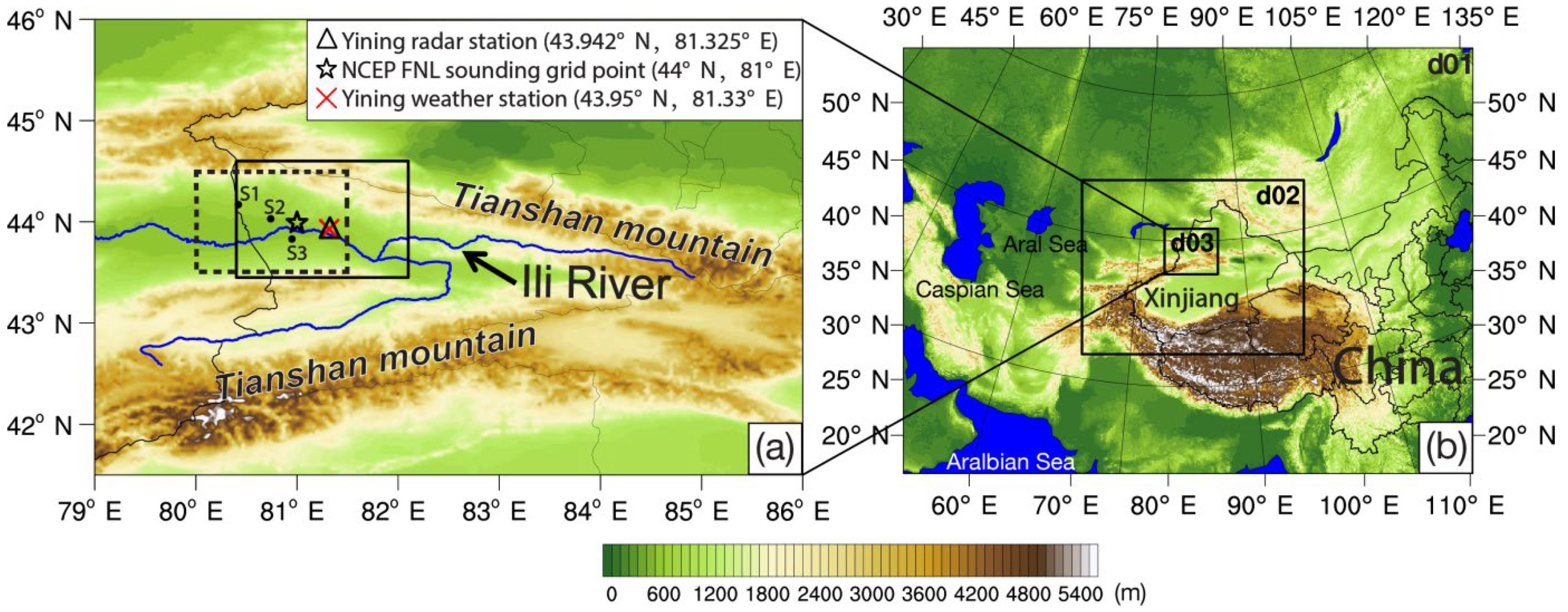
Severe convective storms are considered as one of the most severe disaster-producing weather systems that can cause many serious hazards such as flash flooding, lightning, large hail, severe winds, and tornadoes. For example, an extreme rainfall-producing convective storm occurred over Ili River Valley (IRV) in Xinjiang, Northwest China (Figure 1a) from 0600 UTC 16 June to 2200 UTC 17 June 2016. A number of weather stations had recorded high precipitation exceeding 96 mm, with the most intense precipitation of 151.3 mm occurring in Boerbosong station in Maza Village of Yining County. Specifically, the daily precipitation at Nileke station (68.4 mm) broke the record in the past, and that of Gongliu station (69.5 mm) reached the second highest in its history. This rainstorm event caused severe economic losses of nearly 600 million CNY, with the disaster-affected population exceeding 70,000 [1]. Such an extreme rainstorm is rare in Xinjiang which considered as one of the most arid and semi-arid regions in China.

Although great progress has been made in understanding the life cycle and structure of convective storms, the convection initiation (CI) (i.e., initial formation of a deep convective cloud) remains a scientifically challenging problem, and accurately predicting the CI is one of the weak links in forecasts of convective storm activity, presenting a significant challenge for forecasters [2,3,4,5,6,7,8,9,10].

CI has been studied extensively around the world [3,5,11,12,13,14], as it is crucial to the organization and development of convective storms. Based on over 55,000 CI cases, Lock and Houston [3] concluded that there were four primary factors controlling the occurrence of CI, that is, buoyancy, inhibition, dilution, and lift. They stated that the lift appeared to be the most often factor that plays a crucial role for CI. As has been shown in previous field campaigns {such as the Convective Initiation Downburst Experiment (CINDE) project [15,16], Convection and Precipitation/Electrification (CaPE) project [17,18,19], International H₂O Project (IHOP_2002) field experiment [13,14], and Plains Elevated Convection At Night (PECAN) field project [20]}, the lift is usually induced by various convergent boundaries in the planetary boundary layer (PBL), including gust fronts (i.e., cold pool outflow boundaries), sea-breeze fronts, drylines, terrain-induced boundaries, gravity waves, bores, and horizontal convective rolls (HCRs).

HCRs are defined as linearly organized, quasi-two-dimensional counter-rotating horizontal vortices that commonly occur within the PBL, and their signatures are manifest as cloud streets and linear clear-air radar reflectivity bands that are usually prominent at midday and early afternoon [21,22,23,24,25]. HCRs influence boundary layer circulations, boundary layer structure, and CI [25]. Many previous studies have identified several mechanisms potentially responsible for creating preferred locations for CI along some low-level convergence boundaries, including the enhancement of vertical lifting through the interaction of HCRs with gust fronts [26], sea-breeze fronts [27,28,29], dryline [30,31,32], and mesocyclones [33,34].

The CaPE project demonstrated that updraft branches of HCRs could sufficiently decrease the level of free convection (LFC) and thus reduce the convective inhibition (CIN) to enable CI through boundary layer forcing [19]. Xue and Martin [32] studied a CI case associated with HCRs and dryline during the IHOP_2002 field experiment over the Central Great Plains of the United States [13] and proposed a conceptual model that emphasized the interaction of the HCRs with the mesoscale convergence zone along the dryline for determining the CI locations. They found that the downdrafts of HCRs and the associated surface divergence play a crucial role in generating localized maxima of surface convergence that induced the CI. Steinhoff et al. [35] investigated responsible factors for rare summertime rainfall over portions of the United Arab Emirates and found that CI generated above updrafts associated with the interaction of HCRs and the approaching sea-breeze front. Luo et al. [36] investigated CI mechanism of a squall line in a Meiyu front in East China and found that, HCRs play a crucial role in determining the locations of CIs. They stated that, surface heating increases the convective instability and causes the development of HCRs. When the condensation process is turned off in the simulation, HCRs are still able to lift the low-level air to super-saturation where CI is expected.

Previous studies on CI associated with HCRs and (or) interactions with other convergence boundaries mainly focused on the related specific details of dynamical, thermal and water vapor characteristics. However, to the authors’ knowledge, there was no previous study reporting the CI-inducing HCRs in the IRV. Furthermore, there were rare studies about the CI associated the HCRs in Northwest China. The purpose of this study is to explore the CI mechanism associated with HCRs in the aforementioned extreme rainfall-producing convective storm over IRV via conduct an in-depth investigation on the synoptic- and meso-scale environmental conditions based on high tempo-spatial resolution numerical modeling.

The rest of this paper is organized as follows. Section 2 gives a brief overview of the severe convective storm over the IRV. Section 3 presents the numerical simulation setup and model verification. The mechanism of CI associated with HCRs is analyzed in detail in Section 4. Finally, a summary and discussion are given in Section 5.

2. Case Overview

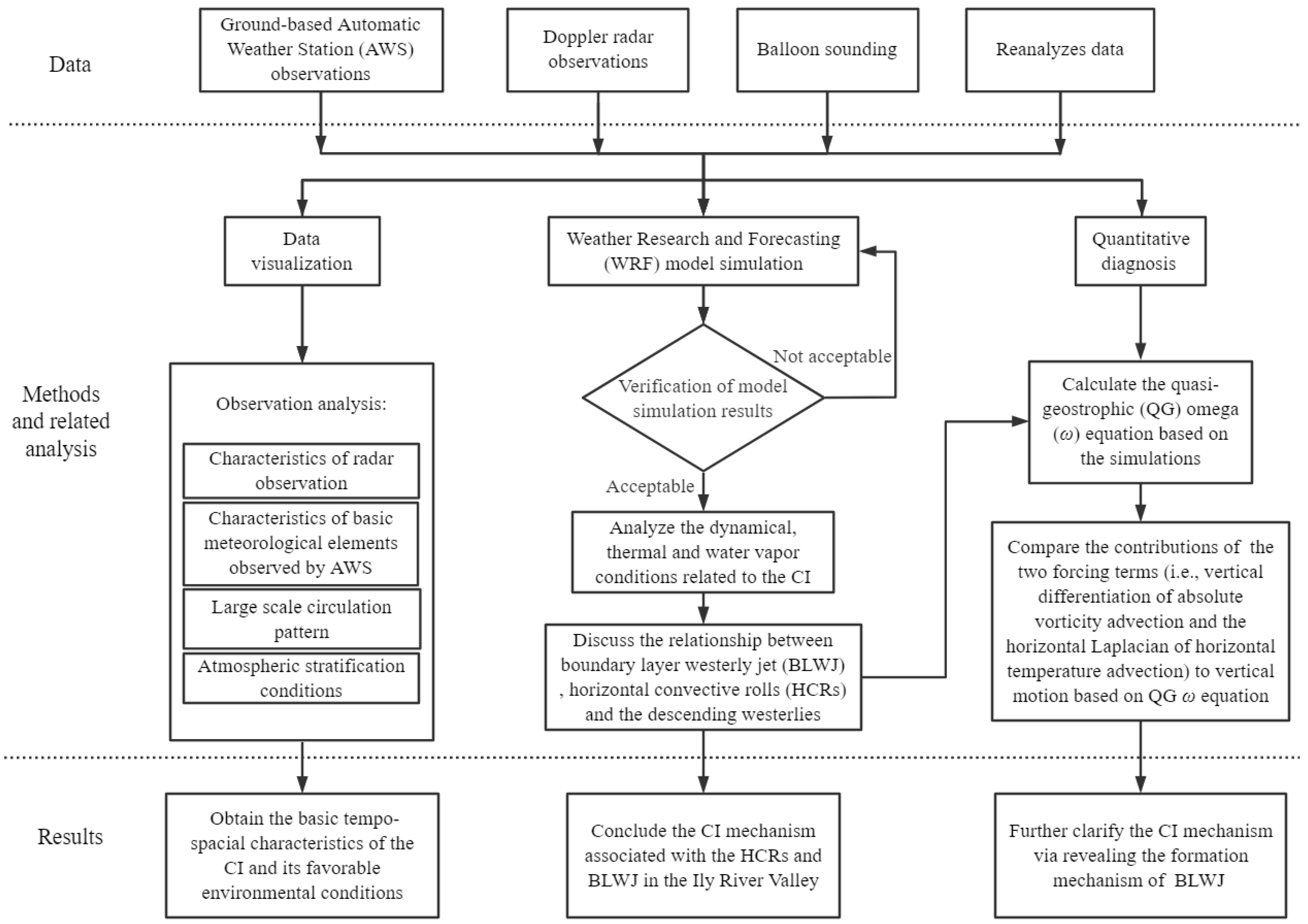
The dataset utilized in present study includes conventional observational data from Doppler radar, ground-based automatic stations (with a temporal resolution of 1 h), and balloon sounding. All these observation data were provided by the National Meteorological Center of the China Meteorological Administration. Besides, we also used National Centers for Environmental Prediction (NCEP) final (FNL) reanalyzes data with 6 h intervals. The methodology used in this study is shown in a flowchart in Figure 2.

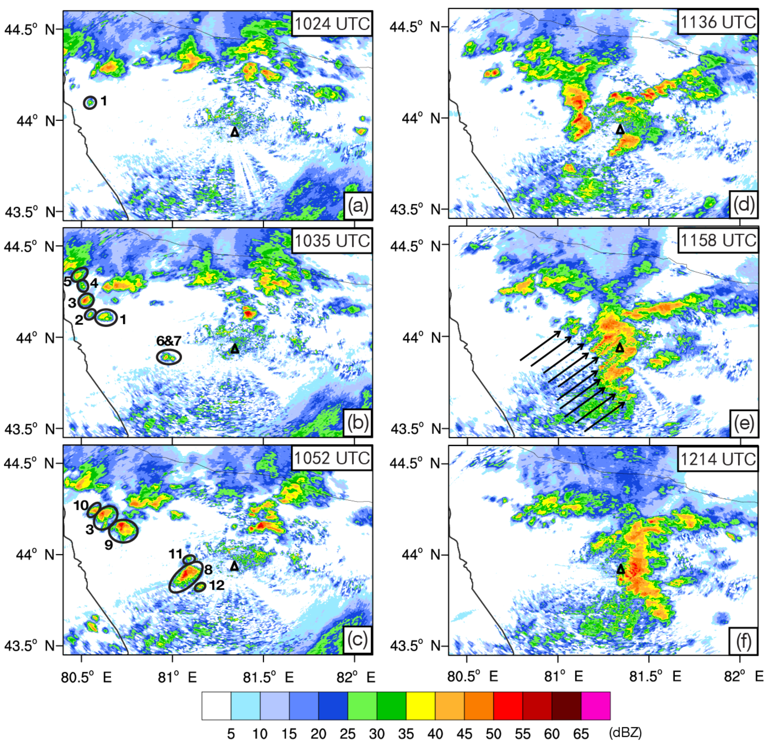
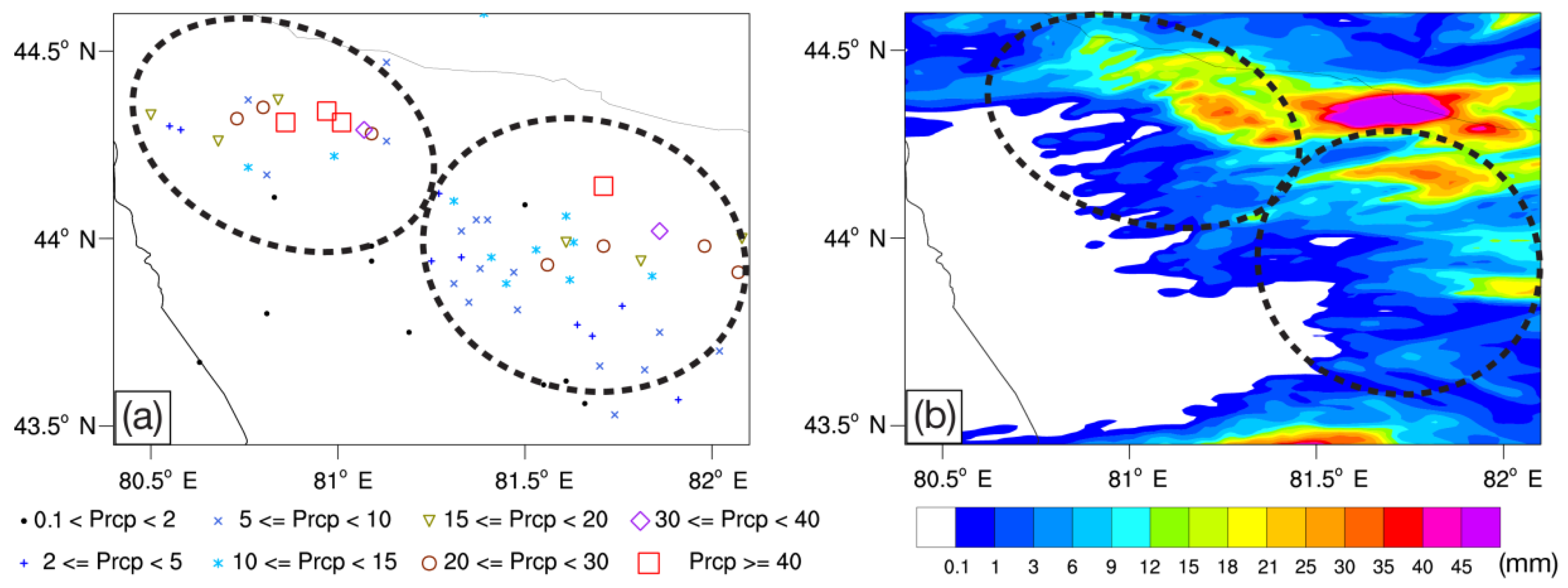
The extreme rainfall-producing convective storm was well captured by the conventional observation. This severe rainstorm process can be divided into two periods. The first period (figure not shown) was from 1200 UTC June 16 to 0300 UTC 17 June 2016. During this period, the precipitation was mainly contributed by the stratus cloud with vertical extension almost <4 km above ground level (AGL). Besides, the composed (i.e., column maximum) radar reflectivity of the clouds was almost <45 dBZ. The second period was from 0900 UTC to 1800 UTC 17 June 2016. During this period, a number of CIs occurred continuously (especially from 1000 to 1200 UTC) in a plain area to the west of the Yining Doppler radar station. The newly initiated convective cells developed significantly in both size and intensity, eventually merged and formed an extreme rainfall-producing mesoscale convective system (MCS). The specific features of this period were well captured by the observation of the Yining radar.

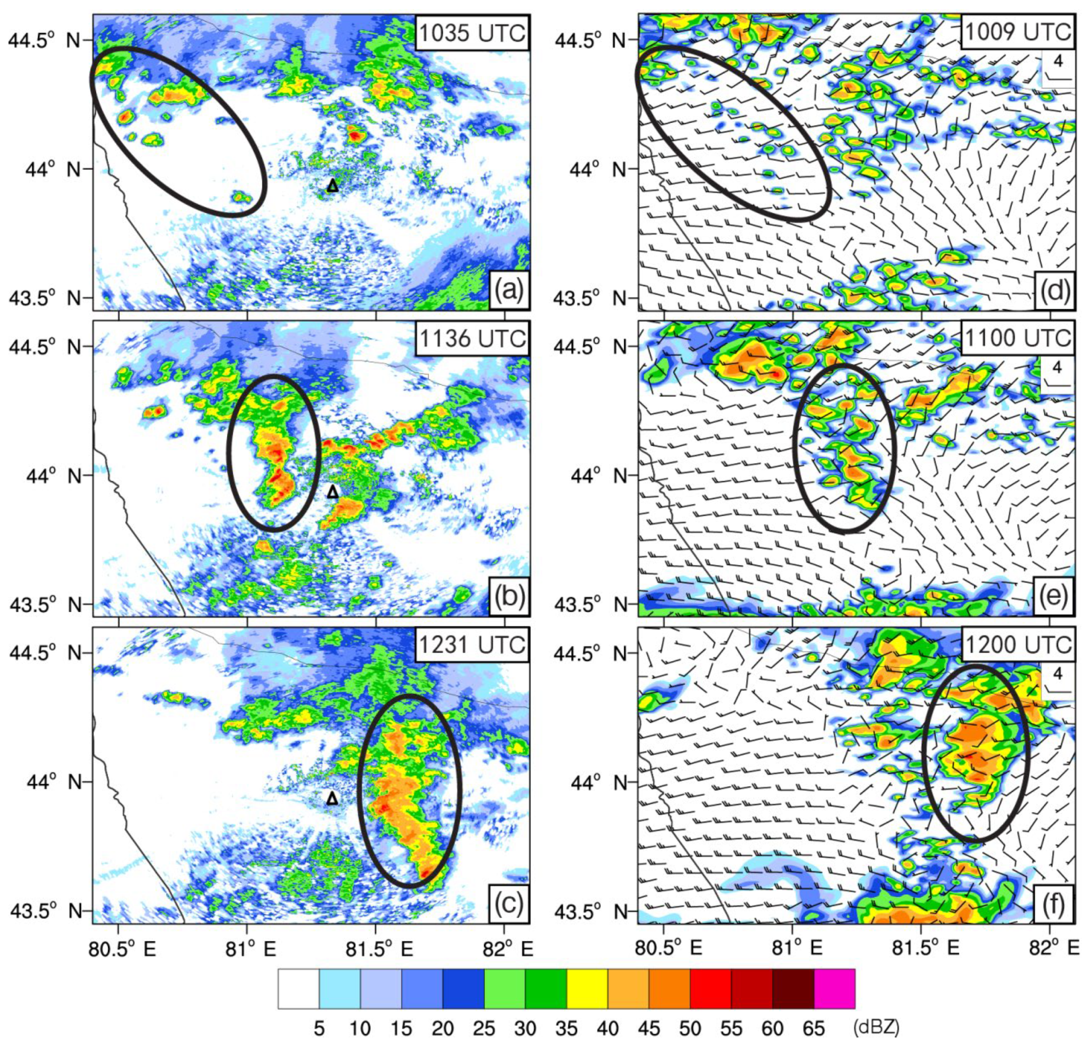
The CI is often defined as the first echo of ≥35 dBZ within a convective cloud [7,37,38,39,40], which is also adopted in this paper. As shown in Figure 3a, there was a CI (denoted as black ellipse and labeled as CI1) occurred at about 90 km northwest of Yining radar station at 1024 UTC. By 1035 UTC (Figure 3b), several other CIs (labelled as CI2–CI7) occurred successively to the northwest and southeast of the CI1. In the following ~1 h (Figure 3c,d), most of the CIs underwent obvious development and merged into relatively large and intense MCS during their continuous eastward movement. The strongest composite reflectivity of the MCS exceeded 60 dBZ (Figure 3d). At 1158 UTC (Figure 3e), the MCS evolved into a more intense and organized form that roughly oriented in north-south direction near the Yining radar station. Furthermore, it is interesting to note that the convection in the MCS showed a quasi-linear arrangement oriented in northeast-southwest direction (indicated by black arrows in Figure 3e) with almost equal spacing. The quasi-linear convective system were most significant in the central part of the MCS, and showed roughly parallel distribution. However, its northern and southern parts were dominated by isolated convective cells (or clusters). The roughly parallel distribution patterns of the convective lines were similar to the morphology of the horizontal convective rolls (HCR) to some extent. By 1214 UTC (Figure 3f), the MCS got further development, and became a north-south oriented linear MCS (i.e., squall line) that was about 80 km in length and 20 km in width. The MCS generated heavy precipitation in many places in the study area during its eastward movement.

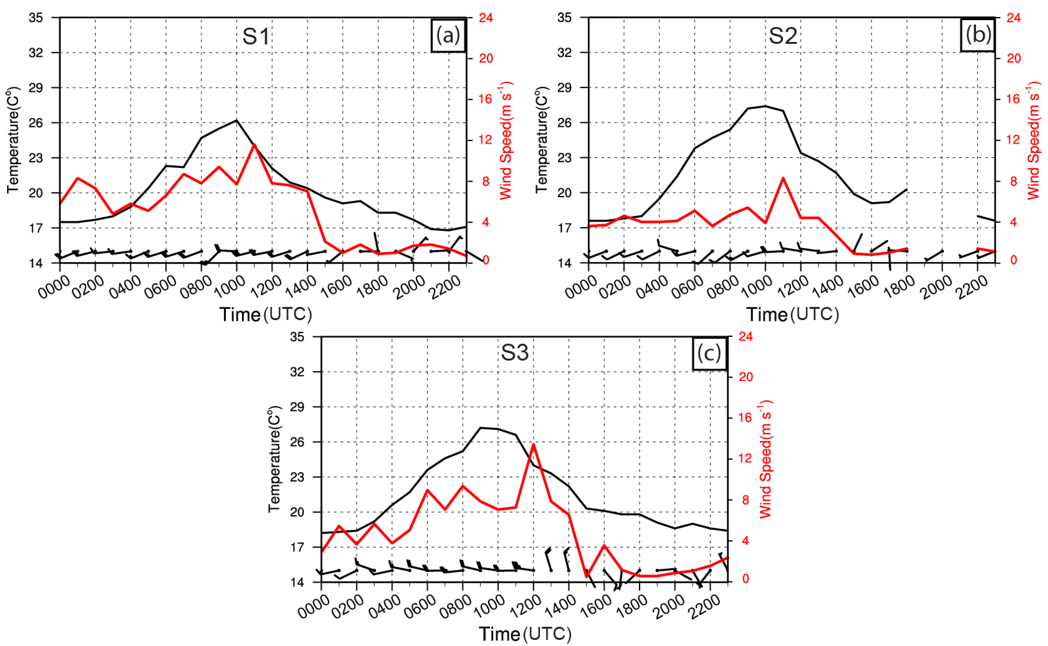
In order to investigate the basic dynamical and thermal characteristics of near-surface layer during the CI period (from 1000 to 1200 UTC), we select three ground-based automatic weather stations to the west of Yining radar station (as shown in S1, S2 and S3 in Figure 1a). As shown in Figure 4a–c, the winds observed by these three stations revealed that the near-surface layer was mainly dominated by westerlies before the CI (i.e., before 1000 UTC). However, during the period when many CIs occurred (i.e., from 1000 to 1200 UTC), the wind speed observed by all three stations increased significantly (the wind direction maintained as westerly). The high wind observed by both S1 and S2 occurred at 1100 UTC, while that of S3 occurred at 1200 UTC (the wind speed of S1 increased from ~8 m s⁻¹ to ~12 m s⁻¹, and that of S2 and S3 increased from ~4 m s⁻¹ to ~8 m s⁻¹, and from ~8 m s⁻¹ to ~14 m s⁻¹, respectively). Consequently, it can be inferred that near-surface of the study area was affected by a relatively strong westerlies during the CI period. The maximum wind speed observed at stations S1 and S3 roughly reached 12 m s⁻¹. Therefore, these westerlies can be called as boundary layer westerly jet (BLWJ). There was 1 h time lag between the occurrence of the BLWJ in S3 and that of S1 and S2, which is likely due to the relatively east geographical location of the S3, such that the arrival time of the leading edge of the BLWJ was later than that of the other two stations (S1 and S2). After 1200 UTC, the wind direction of all three stations showed significant irregular changes, which reflected the wind field transformation caused by the convective system. In addition to the wind changes, the temperature observed by all three stations showed significant decline of about 4–5 °C (temperature of S1 dropped from ~26 °C to ~22 °C, and that of S2 and S3 dropped from ~27.5 °C to ~23.5 °C, and from ~27 °C to ~24 °C, respectively) during the CI period. It can be inferred that, the BLWJ provided cold advection to the study area.

Environmental Conditions

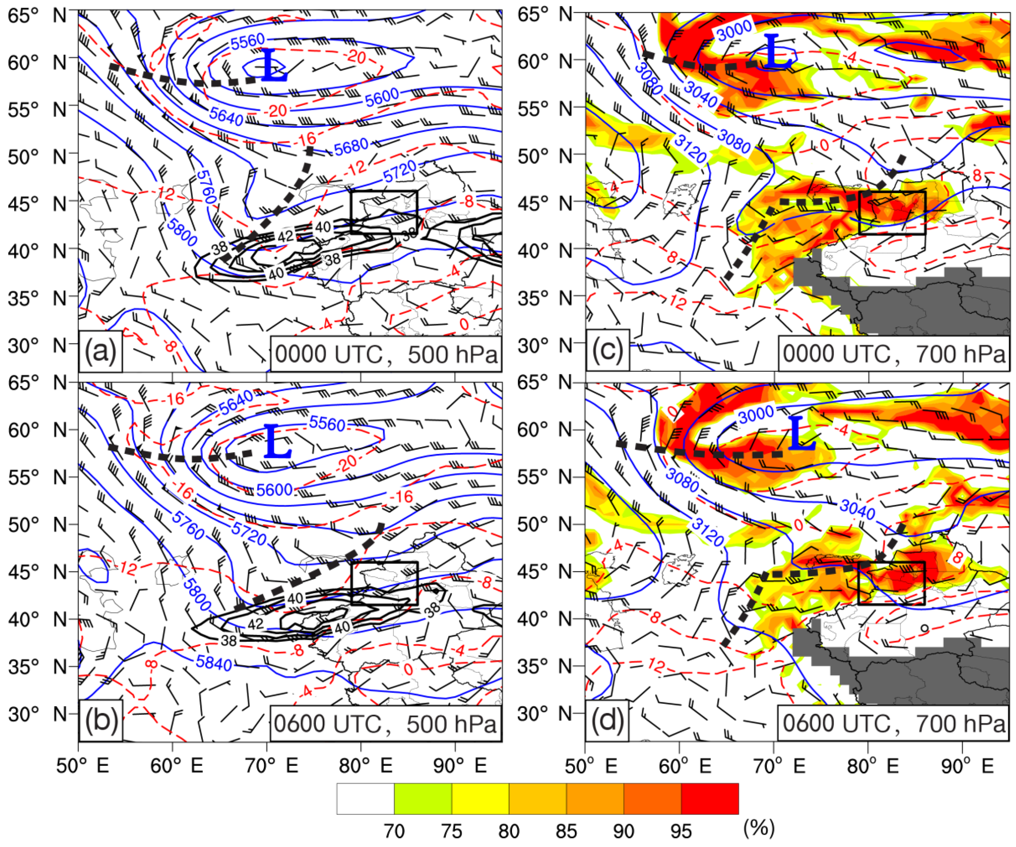
In order to examine the environmental conditions of this severe rainstorm, the 6-hourly, 1 × 1 gridded National Centers for Environmental Prediction (NCEP) Final (FNL) analysis data set (https://rda.ucar.edu/datasets/ds083.2/ (accessed on 25 July 2021)) was used. At 1200 UTC 16 June 2016 (figure not shown), the Central Asian low-pressure system was located over the Central Asian region between the Aral Sea and Balkash lake, and the study area was controlled by the southwesterlies of the vortex. By 0000 UTC 17 June (Figure 5a), the strong northerlies on the west side of the west Siberian low-pressure system (indicated by “L”) delivered intense cold air advection to the upstream region of the study area. The previous Central Asian low-pressure system evolved into a moderately intense trough (indicated by southern dashed line) and gradually moved to the southeast. Besides, there was an upper-level westerly jet at 200 hPa located to the southwest of the study area. Therefore, the upper level (about 200 hPa) over the study area was dominated by a divergent flow which occurred on the left side of the exit area of the jet stream. At 0600 UTC 17 June (Figure 5b), the northern half of the trough moved significantly faster than the southern part and evolved into a quasi-transverse short wave trough along the northeast-southwest direction. The short-wave trough moved over the northwestern edge of the study area and brought more southwesterlies to the study area. Meanwhile, the upper-level westerly jet at 200 hPa slightly intensified (the maximum wind speed in the jet core exceeded 45 m s⁻¹) and moved a little bit eastward, continuously generating upper-level divergence over the study area.

The lower troposphere at 700 hPa at 0000 UTC 17 June (Figure 5c) presented two short wave troughs located mainly under the moderately intense trough at 500 hPa. However, the northern short-wave trough was almost located near the northwestern part of the study area. Its northern part reached near the border area between Northern Xinjiang and Kazakhstan, showing a distribution along the northeast-southwest direction. There were northerlies on the north side of this short-wave trough, while its south side was dominated by westerlies. Therefore, a relatively strong convergence was formed by this low-level trough. Meanwhile, the westerlies to the south of this trough transported moist air (relative humidity exceeding 75%) to the study area. The other short-wave trough in the south was located almost the same place as the southern half of the 500-hPa trough. By 0600 UTC (Figure 5d), both of the short-wave troughs had slightly moved eastward, especially the northern one moving closer to the northwest of the study area. At this time, both of the study area and its upstream region to the west were still dominated by relatively moist westerlies. In general, the upper-level divergence induced by 200-hPa upper-level westerly jet, mid-tropospheric cold advection behind the Central Asian low pressure trough, and the low-level convergence and water vapor transport associated with the 700-hPa short wave trough provided a quite favorable condition for the formation of the severe convective storm.

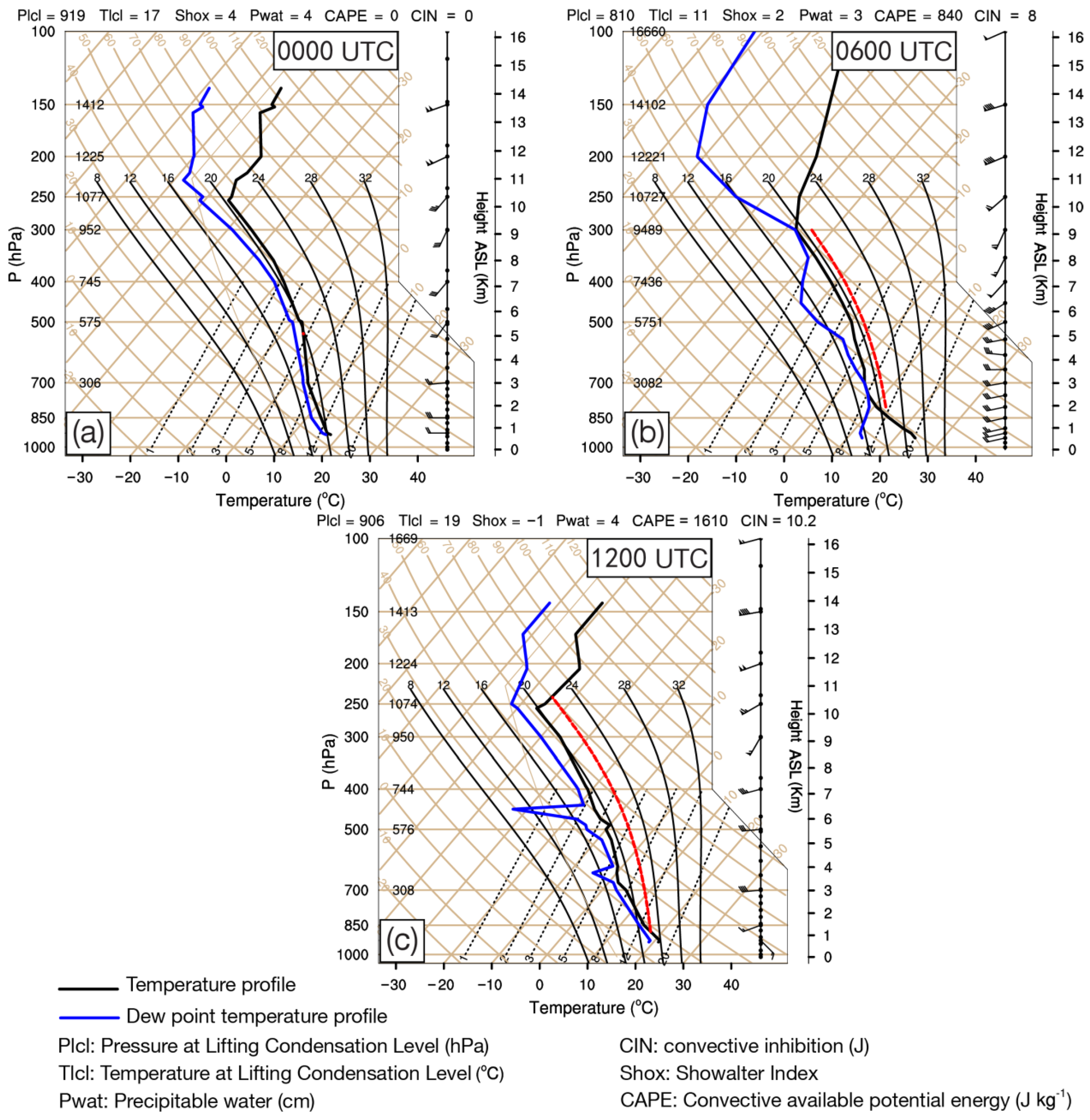
An observational analysis of sounding at 0000 UTC 17 June (Figure 6a) revealed that there was no convective available potential energy (CAPE) and convection inhibition (CIN) in the study area. The Showalter index was 4, which indicated that thunderstorm was unlikely to occur here. However, the precipitable water was not small (reaching 4 cm), and the pressure and temperature of the lifted condensation level (LCL) were 919 hPa and 17 °C, respectively. Besides, the near surface air was rather wet, showing a dew point depression (T-Td) was about 1 K. Furthermore, the whole atmosphere below 300 hPa showed relatively moist condition with dew point depression less than 4 K. In addition, there was a significant vertical shear of horizontal wind that indicated by an enhancement of the wind speed with height at lower troposphere below ~1.5 km above sea level (ASL). The wind speed increased significantly with height at about 0.9–1.5 km (ASL) (increased from ~8 m s⁻¹ to ~12 m s⁻¹), but the wind direction remained as westerly. At the height of 700–500 hPa, the wind direction rotated counterclockwise with height, indicating cold advection. (Since the time interval of conventional radiosonde observation is 12 h, there was no radiosonde observation at 0600 UTC, therefore we used the NCEP FNL data at (44° N, 81° E) as a substitute radiosonde data).

By 0600 UTC (Figure 6b), the CAPE increased to 840 J kg⁻¹, while the CIN showed a very slight increase (reaching to 8 J kg⁻¹). Besides, the Showalter index decreased to 2, indicating the intensification of the instability. Furthermore, the LCL was elevated to some extent (i.e., the pressure and temperature of the LCL were 810 hPa and 11 °C, respectively), and the precipitable water decreased to 3 cm. The near surface air became relatively dry (dew point depression reaching ~7 K). Furthermore, the layer of about 800–750 hPa was almost saturated, while the mid-upper level (500–400 hPa) was obviously dry, showing a dew point depression of ~10 K. Besides, there was a similar counterclockwise rotation of the wind direction with height between 600 and 300 hPa, indicating that the relatively intense cold advection was continuing at this time. Observed sounding at 1200 UTC 17 June (Figure 6c) showed that the CAPE further increased to 1610 J kg⁻¹, while the CIN was still relatively small (10.2 J kg⁻¹). Besides, the Showalter index further decreased to −1, and the LCL decreased significantly (i.e., the pressure and temperature of the LCL were 906 hPa and 19 °C, respectively), along with a slight increase in the precipitable water (reaching to 4 cm). All these indexes implied that the instability increased significantly, and thunderstorm was rather likely to occur here. The atmosphere at about 450 hPa was very dry, showing dew point depression of up to ~20 K. However, the layer of about 400–250 hPa and 850–700 hPa almost remained relatively wet (dew point depression <5 K). At the same time, there was still cold advection in the level of 400–300 hPa. The vertical shear of horizontal wind between 1.5 and 3 km (ASL) was increased significantly (the wind speed increased from 6 m s⁻¹ to 16 m s⁻¹). It is clear that the CAPE has been accumulated with time over the study area before the CI as well as during the development stage of convection. Additionally, the atmospheric stratification, the dry and cold air at the upper level coincided with relatively wet and warm air below, which were very conducive to the CI and development of the convective storm. In the next section, we will further study the mechanism of the CI by using high spatio-temporal resolution simulation data.

3. Numerical Simulation

3.1. Setup of Numerical Experiment

The simulation was performed by using the Weather Research and Forecasting (WRF) model (V4.0), with the Advanced Research dynamics core (ARW) [41]. The model was configured with two-way nested triple-level domains at horizontal grid spacings of 9 km, 3 km, and 1 km, respectively (Figure 1b). The innermost domain (d03) fully covered the area where the convective storm of interest occurred (Figure 1a). There were 50 vertical levels (terrain-following) from the surface to the model top at 50 hPa. For all three domains, the model physics adopted the WRF Single Moment 6-class (WSM6) microphysics scheme [42], Yonsei University (YSU) planetary boundary layer (PBL) scheme [43], The Rapid Radiative Transfer Model for GCMs (RRTMG) longwave and shortwave radiation schemes [44], Noah land surface model scheme [45]. Besides, the Kain-Fritsch scheme [46] was used for cumulus parameterization in domains d01 and d02, while it was turned off in domain d03. (Above physical parameterization schemes were selected as the most appropriate combination based on the results of a dozen experiments.) The initial and boundary conditions were provided by using the 6-hourly NCEP FNL reanalysis data with a resolution of 1° × 1°. All domains were initialized at 0600 UTC on 17 June 2016 and integrated for 18 h. The time intervals of the output data of d03 were 3 min.

3.2. Verification of Simulation

In order to establish the credibility of the simulation, we compare the simulated composite reflectivity and 6-h accumulated precipitation with their observational counterparts in the following. As shown in the simulated composite reflectivity at about 1009 UTC (Figure 7d), several CIs (as shown in the black ellipse) occurred continuously in the plain area about 40–90 km to the northwest of the Yining radar station. The location and pattern of these CIs were in consistent with the radar observation at 1035 UTC (indicated by the black ellipse in Figure 7a), while the time of CI in simulation was about 0.5 h earlier. In the following ~1 h, several other CIs took place successively in the simulation, and most of them merged and significantly developed during their continuous eastward movement. At 1100 UTC, they formed a relatively low-organized MCS that roughly oriented in north-south direction (as shown by the black ellipse in Figure 7e). By 1200 UTC (Figure 7f), the intensity of the MCS was roughly in agreement with the observation (the maximum composite reflectivity reaching 50 dBZ), while it was not so well organized as the observation. Its location was displaced eastward by about 0.2°, and its horizontal spatial scale was a little bit smaller than observation (Figure 7c). In general, the basic characteristics of the CIs and associated MCS in simulation agreed reasonably well with the observation despite some slight biases in time, location and morphology (see

Table 1. The basic features of the CI, MCS and precipitation in simulation and observation.

	Time of the Earliest CI	Location of the Earliest CI	Horizontal Scale of MCS (Length)	Intensity of 6-h Accumulated Precipitation
Simulation	1009 UTC	43.85° N–44.5° N, 80.58° E–81.2° E	~60 km	~30–40 mm
Observation	1035 UTC	43.85° N–44.5° N, 80.45° E–81.0° E	~85 km	~40–50 mm
Deviation	26 min	~0.2° (eastward)	~25 km	~−10 mm

).

Figure 8 shows the 6-h accumulated precipitation observed by the ground-based automatic weather stations and that of model simulation. Due to the complex terrain of Tianshan mountain on both sides of the IRV, the distribution of automatic weather stations in this area is not uniform, and several common interpolation methods (e.g., Cressman Interpolation, Natural Neighbor Interpolation, Inverse Distance Weighted Interpolation, and Tension Splines Interpolation) we had tried to interpolate the observed 6-h accumulated precipitation could not provide a satisfying result. Therefore, we used different symbols to represent the intensity of accumulated precipitation at each station. As shown in Figure 8a, the distribution of the observed accumulated precipitation roughly showed a zonal distribution along the northwest-southeast direction in the IRV. Meanwhile, two large precipitation areas can be seen (indicated by the two ellipses in Figure 8a) in the middle and northern parts of the IRV. The overall pattern of the simulated precipitation (Figure 8b) also roughly showed a zonal distribution along the northwest-southeast direction. Furthermore, two heavy precipitation areas (see two ellipses in Figure 8b) can also be identified. There was an extremely heavy precipitation center (to the north of the eastern ellipse) seen at the middle of the high elevation area on the Tianshan mountain in the simulation. However, the corresponding heavy precipitation center over the same region on the Tianshan mountain was not found in the observation. Thus, it was not considered. The intensity, pattern, and locations of the simulated 6-h accumulated precipitation were consistent with that of observation. Therefore, it is believed that the simulation results well captured the basic characteristics of precipitation in the CI period, despite some bias in intensity (see Table 1).

In general, the overall evolution of the CI and related MCS as well as the 6-h accumulated precipitation was well reproduced by the WRF simulation (especially for the CI process in the area west of Yining radar station). Therefore, the model output was considered to be reliable for the further analysis of mechanism of the CI.

4. Convection Initiation

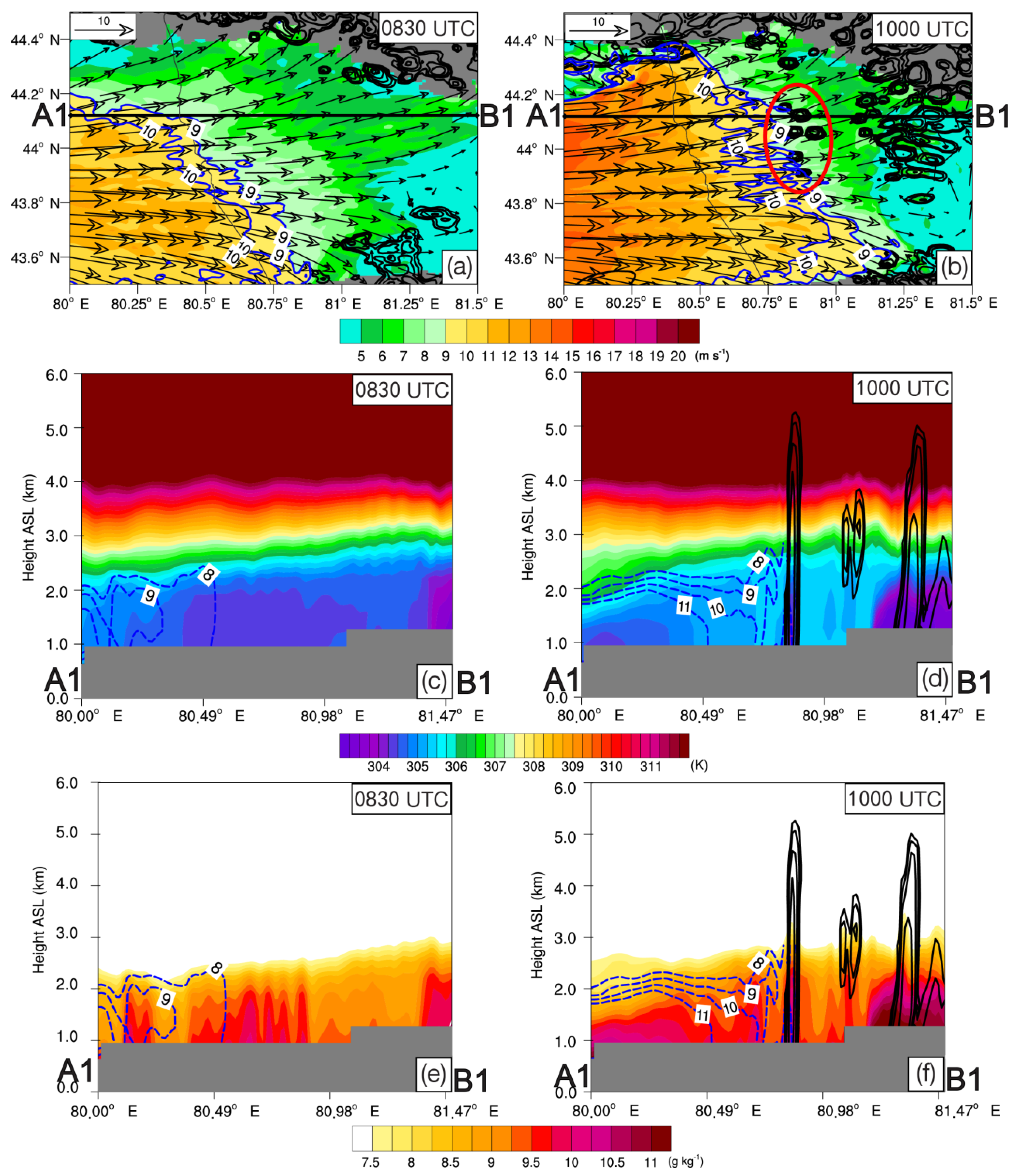
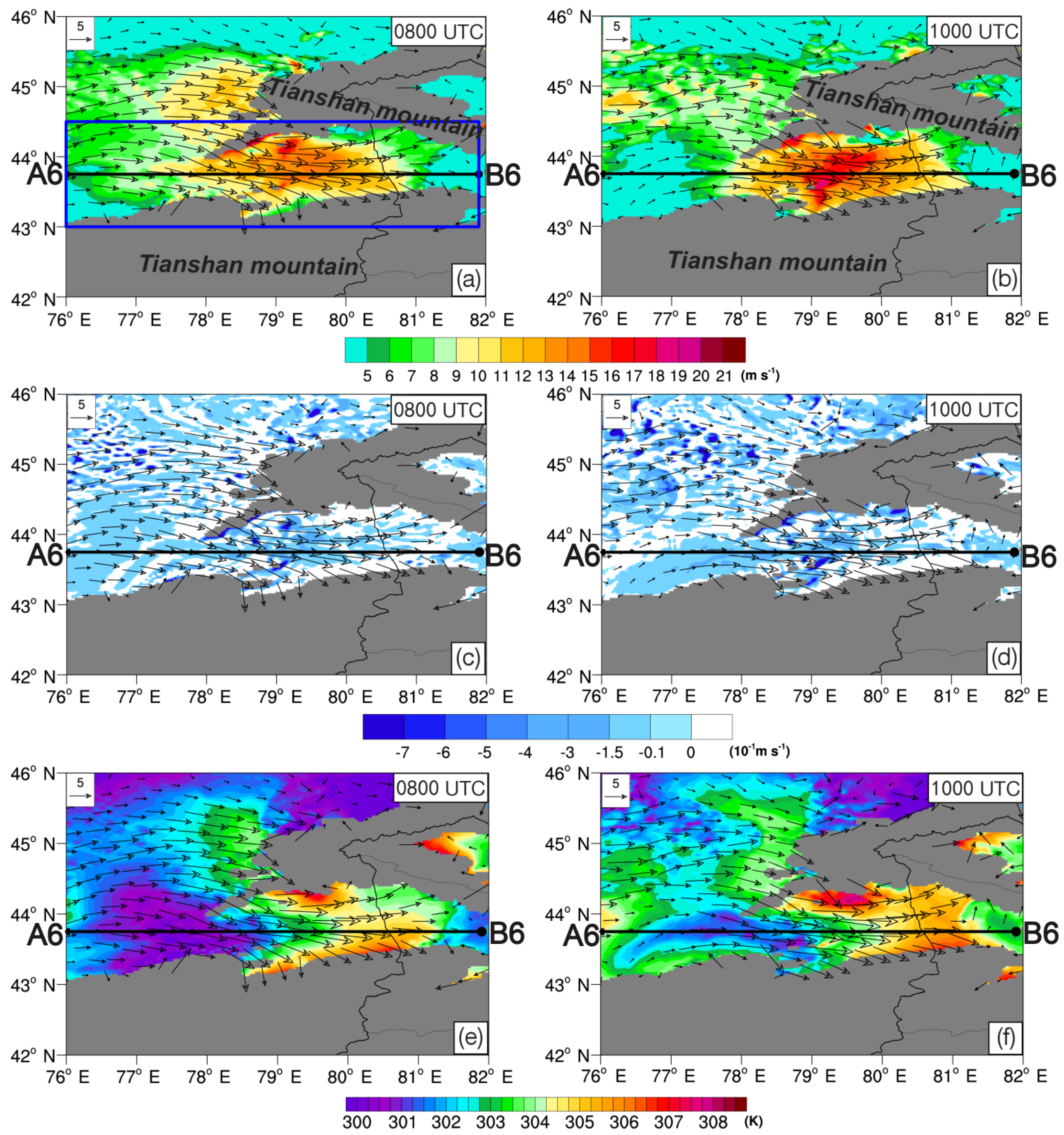
Firstly, the dynamical, thermal, and water vapor conditions of the area before the CI are analyzed. It can be found from the horizontal wind field at the height of 1500 m ASL (Figure 9a,b) that the IRV was affected by a BLWJ in the period before the CI (about 0800–1000 UTC), and the maximum horizontal wind speed exceeded 14 m s⁻¹. The simulated BLWJ almost showed the same characteristics as its observed counterpart as reflected by the winds of ground-based automatic stations (Figure 4) and the sounding (Figure 6). It further indicates that the characteristics of the near-surface (or low level) wind field in the simulation were consistent with that of observation. In addition, it is also found that the main CIs of interest occurred near the isotach of about 9–10 m s⁻¹ in front of the BLWJ (as shown by the red ellipse in Figure 9b). The vertical profile of potential temperature during 0830–1000 UTC showed that (Figure 9c,d), the potential temperature in the low level below ~1.2 km AGL in front of the BLWJ increased from ~304 K to 306 K, indicating that there was an obvious warming in the low level. It was probably due to the increase in surface sensible heat flux caused by diurnal variation of solar radiation. This kind of warming in the low level led to an increase in the CAPE, quite favorable for the CI. However, there was an obvious cold air behind the leading edge of BLWJ, entering the IRV along with the BLWJ. The characteristics of water vapor mixing ratio at 0830 UTC (Figure 9c) showed that, the water vapor conditions in the low level below ~1 km AGL were fairly well (i.e., water vapor mixing ratio exceeding 9 g kg⁻¹), which is probably due to the heavy precipitation occurred in the previous day. By 1000 UTC (Figure 9d), the water vapor mixing ratio in the near-surface level in the BLWJ (especially in the area between 80° E–80.4° E) increased from 8.5–9 g kg⁻¹ to 9.5–11 g kg⁻¹, indicating that the BLWJ also brought some moisture into the study area, which is also quite favorable for the CI. Meanwhile, the newly initiated convective cells near the leading edge of the BLWJ underwent rapid intensification, with their vertical extent reaching about 5.5 km ASL.

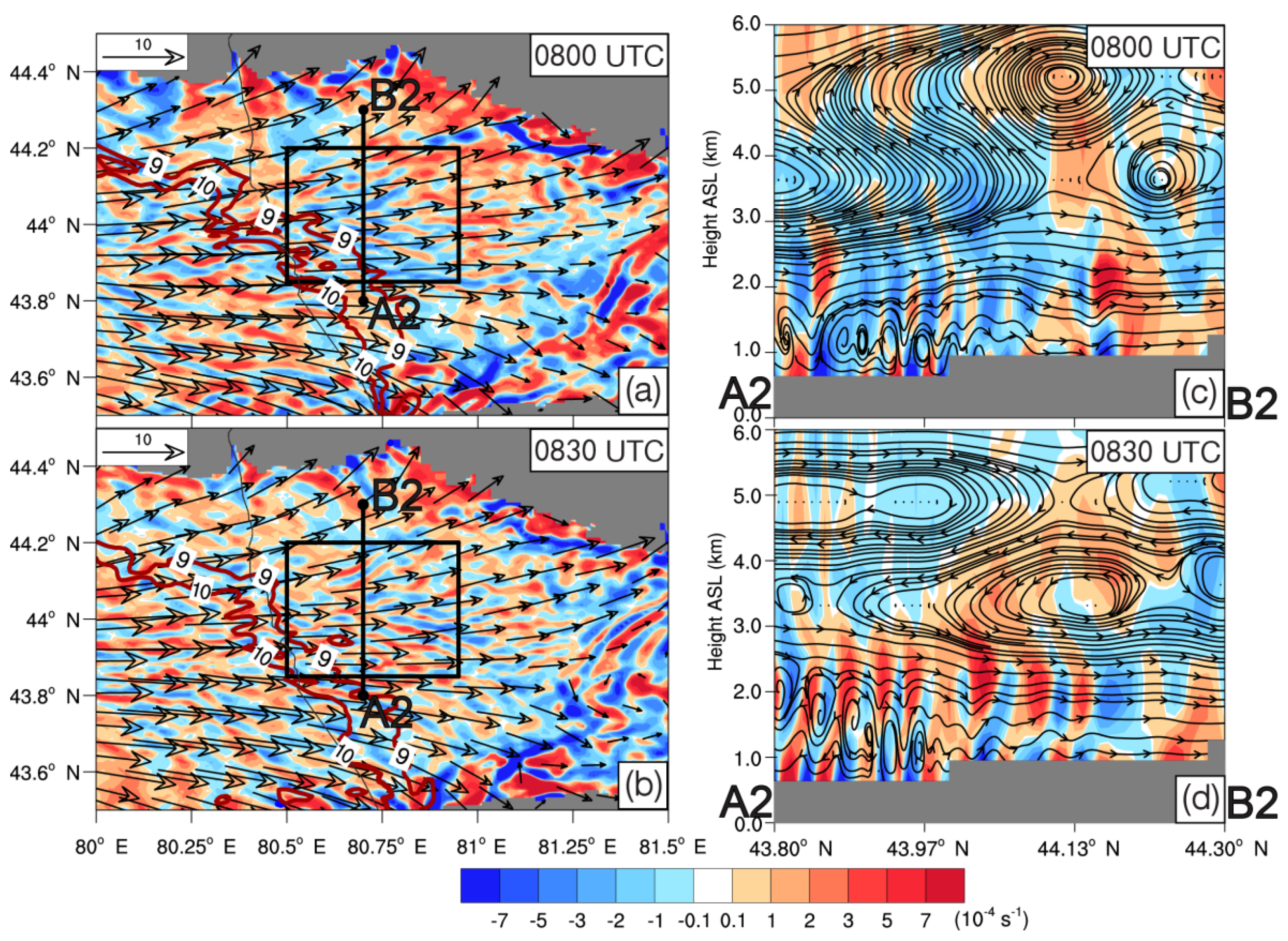
Secondly, in order to further investigate the low-level dynamic features near the area where CIs occurred, the characteristics of horizontal divergence and wind fields in the area are analyzed. As can be seen from the horizontal divergence field at the height of 1500 m ASL (about 700–900 m AGL in the plain area) (Figure 10a), some obvious bands of alternating positive and negative divergence lines began to occur at about 0800 UTC in the area to the east of the 9 m s⁻¹ isotach (indicated by rectangle area) where the CIs mainly occurred. Meanwhile, a number of closed vortex circulations can be found (Figure 10c) in the low level below ~1.8 km ASL (~1.1 km AGL) in the southern half part of the vertical cross section along the line A2B2. By 0830 UTC, the intensity of the alternative positive and negative divergence lines increased to some extent (Figure 10b). Besides, the closed vortex circulations had underwent a significant enhancement (Figure 10d), e.g., the vertical depth of the closed vortices extended to about 2.2 km ASL (about 1.5 km AGL), along with the enhancement of the positive and negative horizontal divergence between these vortices. These closed vortex circulations in the vertical cross section indicated that there were HCRs occurred and intensified with time before the occurrence of CIs in the area ahead of the BLWJ. (As mentioned in the analyses of Yining radar observation above, the observed MCS showed a number of roughly parallel quasi-linear convective system whose morphology were similar to that of the HCRs (Figure 3e). Although no similar convective lines can be found in the simulated MCS (Figure 7e,f), the above analyses (Figure 10) showed that the HCRs do exist in the simulation.) Furthermore, we also found that most of the CIs occurred in the middle of a positive and negative horizontal vorticity bands (i.e., near the HCRs). Because the main focus of this study is on the mechanism of the CI, we will investigate the influence of the HCRs on the CI in the following.

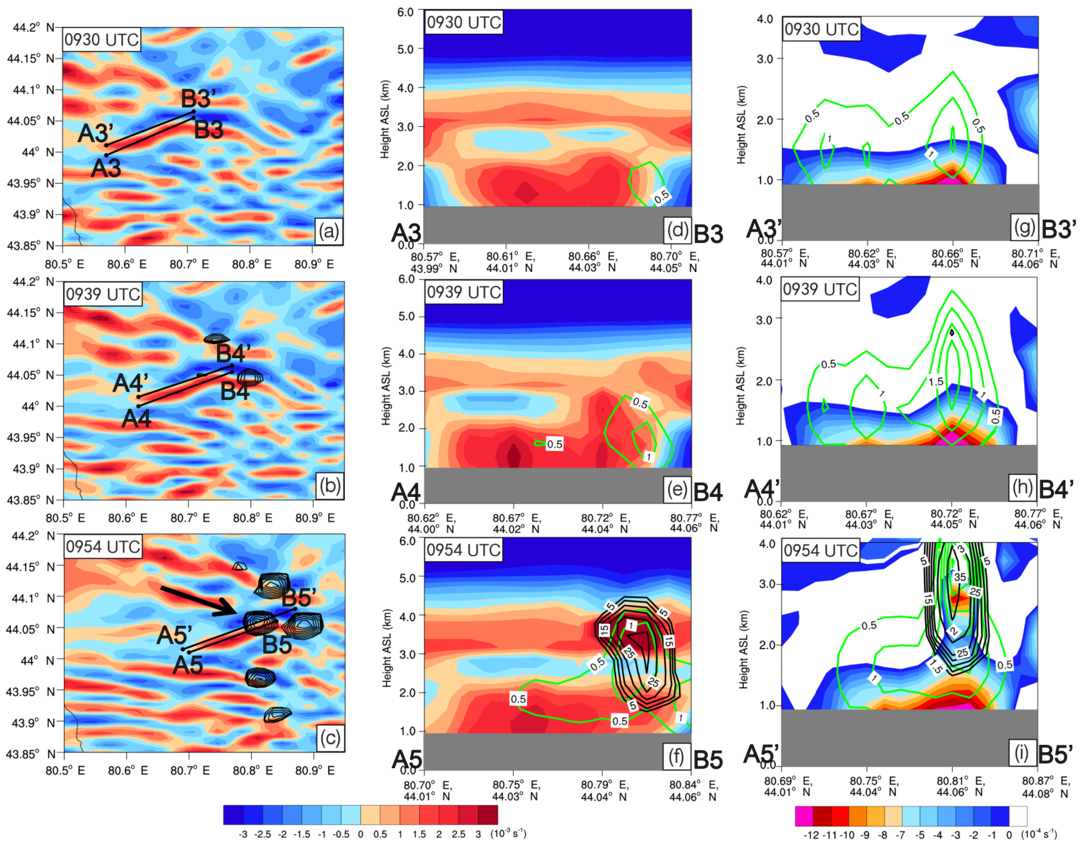
A convective cell initiated at 0954 UTC (indicated by the black arrow in Figure 11c) is selected to analyze its environmental characteristics before CI. At 0930 UTC (i.e., ~25 min before the occurrence of CI, see Figure 11a), the horizontal vorticity on x-direction (abbreviated as HVx) at the height of 1500 m ASL showed an alternative distribution of positive and negative bands in the area west of the CI location. This kind of distribution typically suggests the existence of the HCRs in the horizontal divergence field. At the same time, the vertical cross section along a relatively intense positive HVx band (i.e., selected HCR) showed that (Figure 11d) the intensity of the HVx was up to ~2 × 10⁻³ s⁻¹, and its vertical height reached ~1.2 km AGL. Besides, an updraft (up to ~0.5 m s⁻¹) began to form near the northeastern tip of the selected HCR. It is more noteworthy that there was a strong convergence in the near-surface layer below ~0.5 km AGL in the intermediate area of positive and negative HVx band (i.e., between two HCRs, see Figure 11g), with a relatively strong vertical upward aloft (the vertical velocity exceeding 1.5 m s⁻¹). By 0939 UTC (Figure 11b,e), the selected HCR intensified to some extent (the maximum value of HVx exceeding 3 × 10⁻³ s⁻¹), and the corresponding vertical velocity also significantly increased (exceeding 1 m s⁻¹). At this time, the convergence in the near-surface layer in the area between the two HCRs was further intensified (Figure 11h), with the updraft aloft developed in both size and intensity (i.e., the 0.5 m s⁻¹ isotach exceeding 3.5 km ASL, the maximum updraft in excess of 2 m s⁻¹). At 0954 UTC (Figure 11c,f,i), the CI occurred between the two HCRs, where an intense horizontal convergence was collocated with an updraft aloft (the vertical velocity exceeding 3.5 m s⁻¹). We also analyzed several other CIs and got the same results about the characteristics of their horizontal vorticity, divergence, and vertical velocity (not shown). It can be concluded that, the CIs in this area were triggered by the low-level dynamic disturbance (convergence) induced by the HCRs. Therefore, the roughly parallel quasi-linear convective system in the observed MCS (Figure 3e) were very likely caused by HCRs.

Previous studies [24,47,48,49] suggested that HCRs tend to develop over land in response to moderate sensible heat flux with a parallel alignment of the vertical wind shear vector. Both of these favorable conditions for the formation of the HCRs do exist in our study. The favorable vertical wind shear was mainly contributed by the BLWJ mentioned above. However, it is not clear that how the BLWJ was generated. In order to study the formation mechanism of the BLWJ, the dynamic and thermal characteristics of the upstream area (i.e., to the west of the study area) are analyzed in the next.

The horizontal wind field at 1500 m ASL in the period of 0800–1000 UTC showed that (Figure 12a,b), the wind speed of westerlies increased significantly (the maximum wind speed reaching ~20 m s⁻¹) with time after entering the middle reaches of the IRV. It is probably due to the funneling effect induced by the Tianshan Mountains on both sides of the IRV. Besides, there were obvious large scale descending flows in the middle reaches of the IRV in this period (Figure 12c,d), and the most notable subsidence was up to about −0.7 m s⁻¹. Furthermore, it can be seen from the potential temperature field that (Figure 12e,f), the air mass to the west of the IRV was significantly colder than in the middle reaches of the IRV. Consequently, the westerlies caused quite intense cold advection to the middle and upper reaches of the IRV. The cold advection along with strong westerlies was quite significant in this period, although there was an obvious afternoon warming in the whole area (0800 and 1000 UTC corresponding to about 1300 and 1500 LST, respectively).

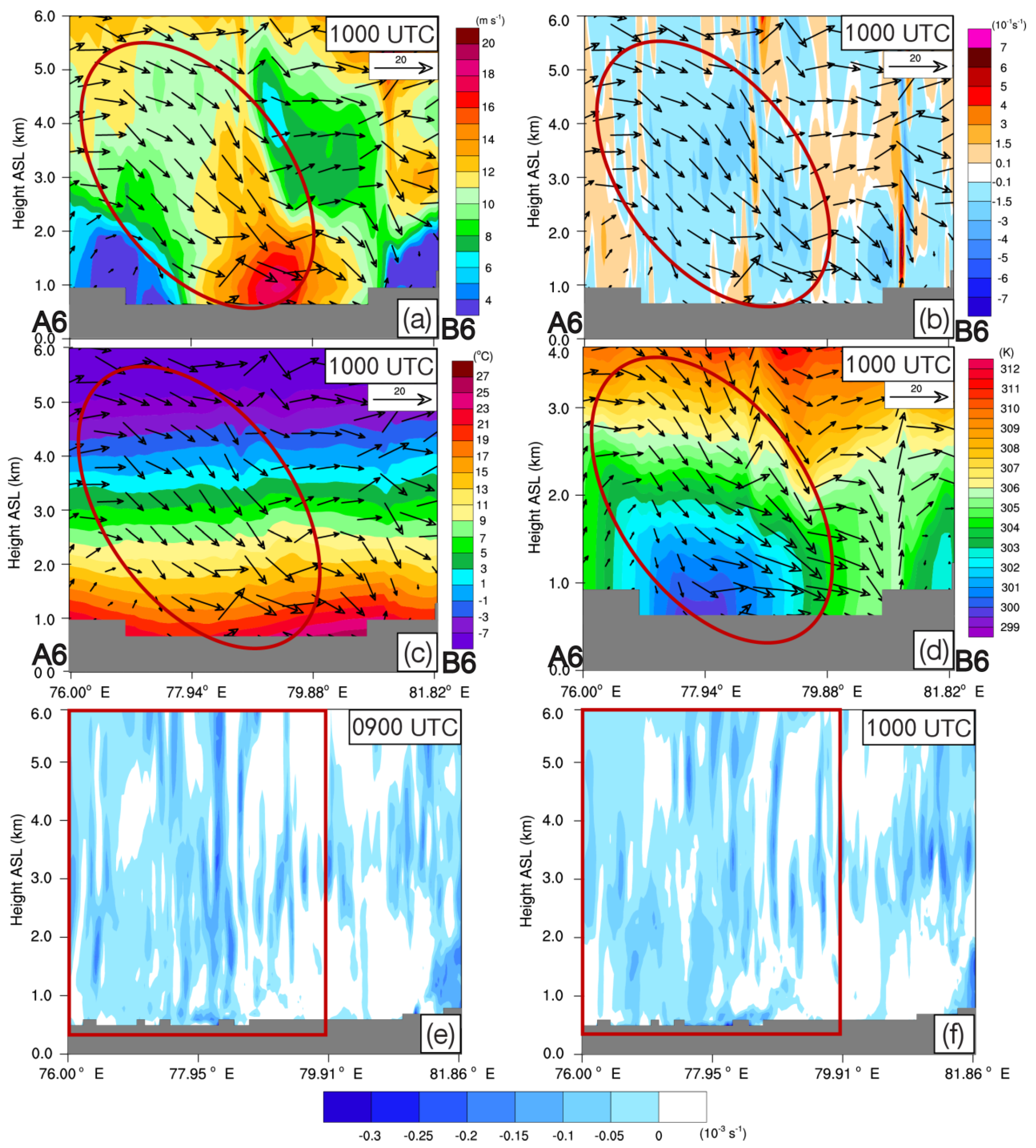
In order to further understand the genesis of the descending westerlies in the IRV, we further analyze the zonal vertical cross section of dynamical and thermal features in the middle reaches of the IRV. It is obvious that, there were gradually increased descending westerlies over the area at about 77° E–80.5° E in mid- to lower troposphere in the IRV. At 1000 UTC (Figure 13a), the wind in this area increased significantly (exceeding ~12 m s⁻¹), and the more intense high wind occurred at the low level below ~2 km ASL, with the maximum wind speed over 18 m s⁻¹. Besides, the wind vector and vertical velocity (Figure 13b) showed that the significant descending westerlies occurred in the level below ~5.5 km ASL (see the red ellipse). The temperature field indicated that (Figure 13c), there was a concave distribution of isotherms along with the descending flow over the area between ~76° E–80.5° E, which was most obvious in the low level below ~3.5 km ASL. Meanwhile, the vertical profile of potential temperature (θ) reflected that (Figure 13d) there were small fluctuations of isotherms in the descending flow, with an intense cold air mass below ~2.5 km ASL. The coldest air mass (with θ < 300 K) was located in the area of ~77.5° E–78° E. Besides, the isotherms on both sides of the central cold air mass were perpendicular to the ground, and the significant descending flow (with high winds) mainly occurred on its east side, which suggested intense eastward cold advection. Consequently, it is clear that there were descending westerlies in the middle reaches of the IRV which could provide cold advection to the study area, and the cold advection in the low level below ~2.5 km ASL can further lead to the descending of the westerlies in this layer. Therefore, as analyzed above (Figure 9a,b), the descending westerlies generated the BLWJ which moved to the study area. The meridional-averaged vertical vorticity in the middle reaches of the IRV (as shown by the blue rectangle in Figure 12a) showed that (Figure 13e,f), there were obvious negative vertical vorticity in the middle to lower troposphere (see the red rectangular) in the period of 0800–1000 UTC (the figure at 0800 UTC not shown). As will be shown below, the relatively intense large-scale negative vorticity was conducive to the generation of the aforementioned descending flow.

In general, the negative vertical vorticity and cold advection in the middle reaches of the IRV combined to induce the descending westerlies in this area, and the wind speed was further strengthened due to the funneling effect in the middle reaches of the IRV, finally leading to the quite intense BLWJ in the study area.

Finally, in order to further investigate the relative contributions of the negative vertical vorticity and cold advection to the descending flow analyzed above, we adopt the adiabatic form of the quasi-geostrophic (QG) omega (ω) equation in the isobaric coordinate system [50], i.e.,

$$\left(\sigma {\nabla }^2+f^2\frac{{\partial }^2}{\partial p^2}\right)\omega =f\frac{\partial }{\partial p}\left[{\overrightarrow{V}}_{\mathrm{g}}·\nabla \left({\varsigma }_{\mathrm{g}}+f\right)\right]-{\nabla }^2\left[{\overrightarrow{V}}_{\mathrm{g}}·\nabla \left(\frac{\partial \varphi }{\partial p}\right)\right]$$

(1)

where $\omega =\frac{dp}{dt}$ is the vertical motion in the isobaric coordinate, $\mathsf{\sigma }=-\frac{\mathrm{RT}}{p}\frac{\partial \ln \mathsf{\theta }}{\partial p}$ is the static stability with R = 287 m² s⁻² K⁻¹ being the specific gas constant, T the temperature, and θ the potential temperature, ∇ and ∇² are the 3-D gradient operator and 3-D Laplacian operator, respectively, f is the Coriolis parameters, ${\overrightarrow{V}}_{\mathrm{g}}$ = (u_g, v_g) is the geostrophic velocity vector, ${\varsigma }_{\mathrm{g}}=\frac{\partial v_{\mathrm{g}}}{\partial x}-\frac{\partial u_{\mathrm{g}}}{\partial y}$ is the relative vorticity, and $\varphi$ is the geopotential height. The QG ω equation is usually used to assess contributions of vertical motion from different physical processes [50,51]. The first term on the right-hand-side (RHS) represents vertical differentiation of absolute vorticity advection (ω₁), while the second RHS term is proportional to the horizontal Laplacian of horizontal temperature advection (ω₂). When the term $\frac{\partial }{\partial p}\left[{\overrightarrow{V}}_{\mathrm{g}}·\nabla \left({\varsigma }_{\mathrm{g}}+f\right)\right]<0$ (i.e., absolute vorticity advection decreases with decreasing pressure (increasing height)) and the term $-{\overrightarrow{V}}_{\mathrm{g}}·\nabla \left(\frac{\partial \varphi }{\partial p}\right)<0$ (i.e., cold advection), it is conducive to the formation of downward motion, and conversely conducive to upward motion. Therefore, the contributions of the two forcing terms (i.e., ω₁ and ω₂) can be qualitatively analyzed to understand the descending flow in the middle reaches of the IRV (i.e., upstream area of the study area).

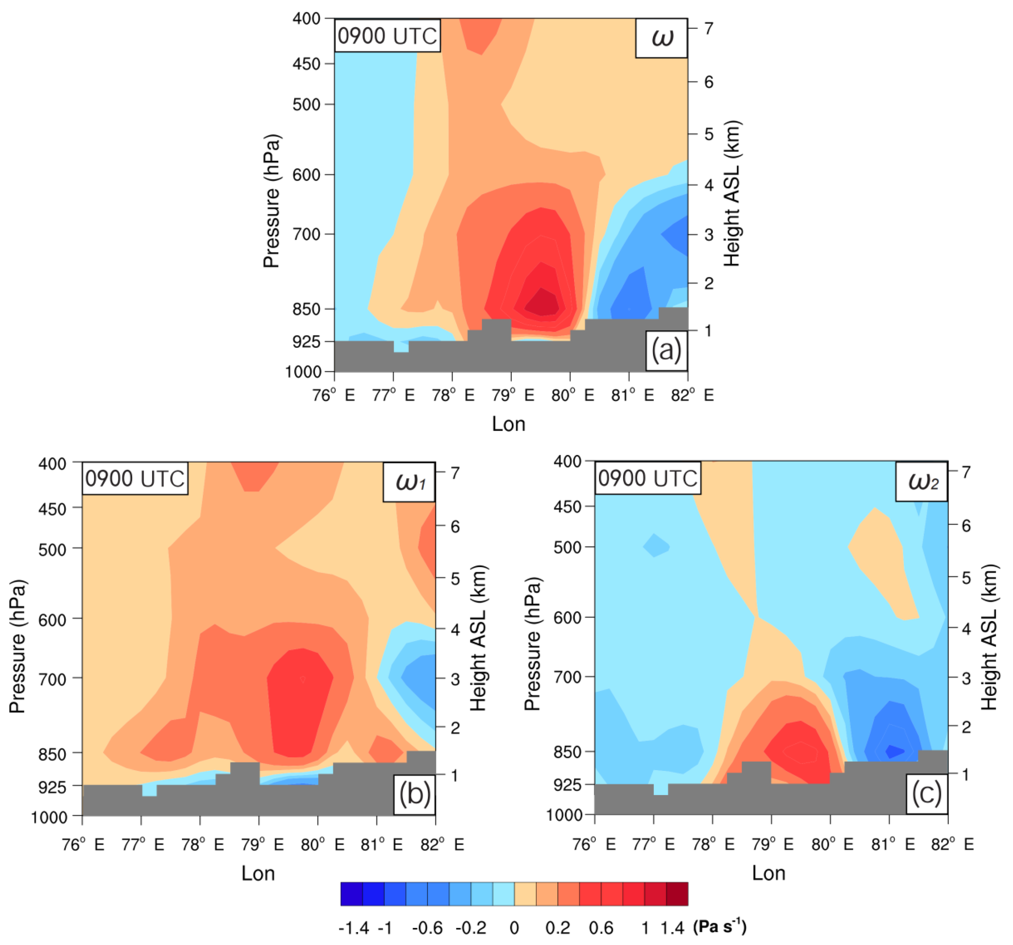
At 0900 UTC (Figure 14a), vertical cross section of the ω shows the significant descending flow over the area between 77° E–80.2° E, with relatively extensive descending (exceeding 0.2 Pa s⁻¹) revealed at the level of mid- to lower troposphere (1~5 km ASL) over the area between 78.3° E–80.2° E. Meanwhile, the ω₁ reflected similar distribution that there was dominant descending flow over the area between 77° E–80.2° E, except for the shallow near surface layer (Figure 14b). Besides, there was a significant descending at the height of 1.3~4 km ASL over the area between 78.3° E–80.2° E, which was very similar to the vertical distribution of ω. Therefore, it can be deduced that the ω₁ made a significant contribution to the ω in mid- to lower troposphere in the middle reaches of the IRV. The ω₂ indicates that there was an extensive descending in the lower troposphere below 3 km ASL in the area ~78° E–80.2° E (Figure 14c). This significant descending of ω₂ was quite coincident with the major extensive descending (exceeding 0.4 Pa s⁻¹) of the ω in the low level below 3.5 km ASL. Consequently, it can be inferred that the ω₂ also exhibited a remarkable positive contribution to the ω in lower troposphere below 3 km ASL.

In general, the qualitatively analysis based on the QG-ω equation shows that the descending flow in the middle reaches of the IRV was mainly dominated by the ω₁, while the descending in the lower troposphere below 3 km (ASL) was controlled by both ω₁ and ω₂.

5. Summary and Discussion

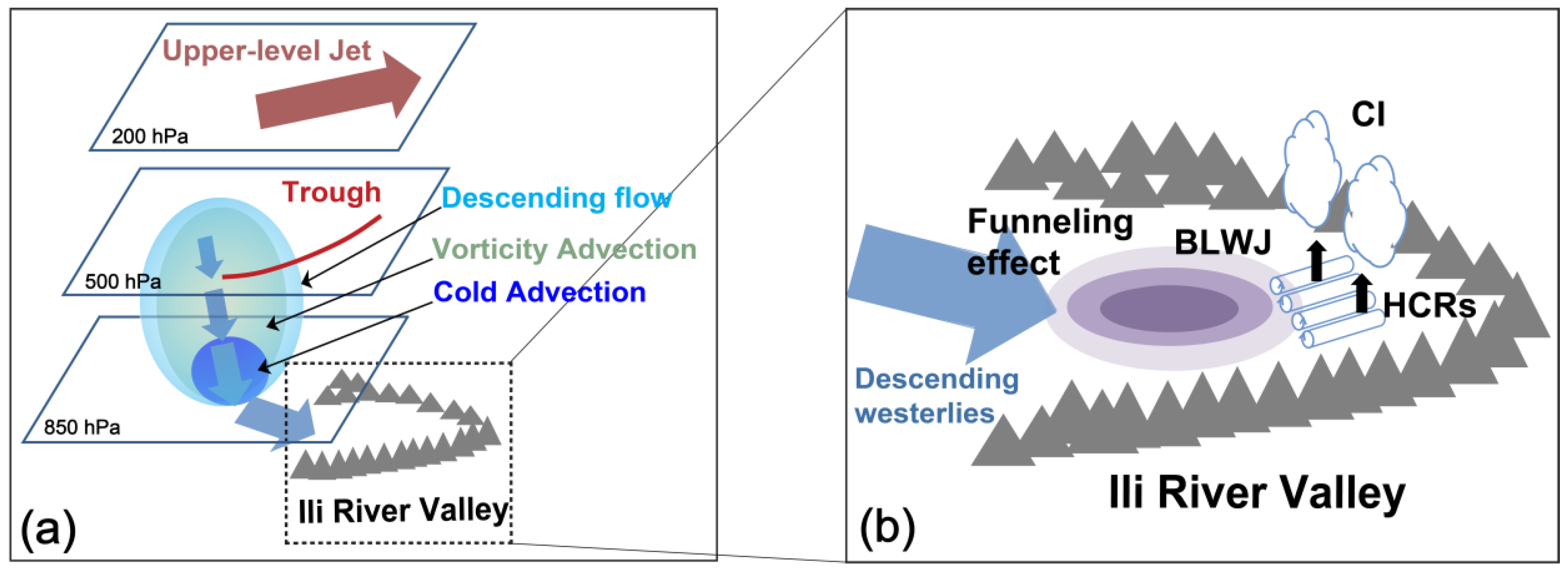
This work can be considered as the first in-depth investigation about convection initiation (CI) mechanism associated with horizontal convective rolls (HCRs) over Ili River Valley (IRV), northwest Xinjiang, Northwest China. Observations of Yining Doppler weather radar showed that a number of CIs occurred repeatedly, and most of them underwent significant intensification both in size and intensity, and finally formed an extreme rainfall-producing mesoscale convective system (MCS, the maximum composite reflectivity of the MCS exceeded 60 dBZ). Wind and temperature characteristics observed by ground-based automatic weather stations revealed that the near-surface layer was affected by a relatively strong boundary layer westerly jet (BLWJ) which caused a temperature drop about 4–5 °C during the CI period. The large-scale circulation pattern and sounding analyzes showed that the upper level divergence induced by upper-level westerly jet, cold and dry advection behind the Central Asian low pressure trough in the mid-upper troposphere, and the convergence generated by the short wave trough and associated significant warm and moist air delivered from west in the lower troposphere provided quite favorable conditions for the formation of the severe convective storm.

This case was simulated using Weather Research and forecasting (WRF) model with a horizontal resolution of 1 km. The WRF simulation well captured the overall pattern and features of the CIs and associated MCS despite some slight biases in time (about 0.5 h early), location (displaced eastward by about 0.2°) and morphology. The dynamical, thermal and water vapor conditions of the study area before the CI showed that, in the period before the CI, the low level below ~1.2 km AGL was relatively wet, and it was warmed with time due to the diurnal variation of solar radiation. Besides, a BLWJ (the wind speed exceeded 20 m s⁻¹) moved to the study area and delivered cold and moist air. Furthermore, there were some HCRs developed ahead of the BLWJ and provided significant convergence (the intensity was up to ~2 × 10⁻³ s⁻¹) in the low level that further induced intense updraft aloft (the vertical velocity exceeded 3.5 m s⁻¹), and eventually led to the CIs. The intense dynamical disturbances in the low level due to the HCRs were mainly responsible for the CIs.

Further investigations revealed that, as the main contributor to the HCRs, the BLWJ was developed due to the funneling effect when the descending air flow entered the middle reaches of the IRV. Furthermore, the descending westerlies in mid- to lower troposphere in the middle reaches of the IRV were generated by the negative vertical vorticity and cold advection. In addition, a qualitative analysis based on the quasi-geostrophic (QG) omega (ω) equation indicated that the descending flow in mid- to lower troposphere in the middle reaches of the IRV was mainly dominated by the vorticity advection, while the descending in the lower troposphere below 3 km ASL was contributed by both vorticity advection and cold advection (see Figure 15).

Nakanishi et al. [52] studied the diurnal variations of PBL in the Wangara experiment [53] using a large-eddy simulation (LES) model. They stated that, as the surface heat flux decreases from late afternoon to evening, an inertial oscillation was initiated and was accompanied by a low-level jet (LLJ) at a height of ~200 m AGL. After 2100 LST, the horizontal advection of warm air due to the LLJ under a large-scale horizontal gradient of temperature destabilizes the residual layer (RL) and consequently induces HCRs, parallel to a vertical wind shear (VWS) vector, between heights of 400 and 1400 m AGL. Similar to the findings of Nakanishi et al. [52], the BLWJ in our case was generated in the lower troposphere near the surface. However, the CI associated with the HCRs occurred in the evening in their case, and there was a warm advection which induced the HCRs. In contrast, the CI in our case occurred in afternoon along with a cold advection associated with the BLWJ. Therefore, there are some uniqueness of our findings in this paper.

The findings in our present work are unique, and they can provide some new insights into the roles of BLWJ and associated HCRs in the mechanism of CI in IRV. However, additional simulations (including sensitivity experiments) will be conducted to further clarify the effects of topography and micro-scale processes which may be related to the CI and development of the deep convection in the IRV in the future.

References

1. Zeng, Y.; Yang, L.M.; Zhang, Y.X. Numerical simulation of mesoscale system during a rare torrential rainstorm process in Ili of Xinjiang. J. Arid. Meteorol. 2020, 38, 290–300. [Google Scholar] [CrossRef]
2. Kain, J.S.; Coniglio, M.C.; Correia, J.; Clark, A.J.; Marsh, P.T.; Ziegler, C.L.; Lakshmanan, V.; Miller, S.D., Jr.; Dembek, S.R.; Weiss, S.J.; et al. A feasibility study for probabilistic convection initiation forecasts based onexplicit numerical guidance. Bull. Am. Meteorol. Soc. 2013, 94, 1213–1225. [Google Scholar] [CrossRef] [Green Version]
3. Lock, N.A.; Houston, A.L. Empirical Examination of the Factors Regulating Thunderstorm Initiation. Mon. Weather Rev. 2014, 142, 240–258. [Google Scholar] [CrossRef] [Green Version]
4. Ukkonen, P.; Manzato, A.; Makela, A. Evaluation of Thunderstorm Predictors for Finland Using Reanalyses and Neural Networks. J. Appl. Meteorol. Climatol. 2017, 56, 2335–2352. [Google Scholar] [CrossRef]
5. Zhang, Y.; Zhang, F.; Stensrud, D.J.; Meng, Z. Intrinsic predictability of the 20 May 2013 tornadic thunderstorm event in Oklahoma at storm scales. Mon. Weather Rev. 2016, 144, 1273–1298. [Google Scholar] [CrossRef]
6. Abulikemu, A.; Xu, X.; Wang, Y.; Ding, J.; Zhang, S.; Shen, W. A modeling study of convection initiation prior to the merger of a sea-breeze front and a gust front. Atmos. Res. 2016, 182, 10–19. [Google Scholar] [CrossRef]
7. Abulikemu, A.; Wang, Y.; Gao, R.; Wang, Y.; Xu, X. A numerical study of convection initiation associated with a gust front in Bohai Bay region, North China. J. Geophys. Res. Atmos. 2019, 124, 843–860. [Google Scholar] [CrossRef]
8. Abulikemu, A.; Ming, J.; Xu, X.; Zhuge, X.; Wang, Y.; Zhang, Y.; Zhang, S.; Yu, B.; Aireti, M. Mechanisms of Convection Initiation in the Southwestern Xinjiang, Northwest China: A Case Study. Atmosphere 2020, 11, 1335. [Google Scholar] [CrossRef]
9. Lin, G.; Grasmick, C.; Geerts, B.; Wang, Z.; Deng, M. Convection initiation and bore formation following the collision of mesoscale boundaries over a developing stable boundary layer: A case study from PECAN. Mon. Weather Rev. 2021, 149, 2351–2367. [Google Scholar] [CrossRef]
10. Zhu, L.; Bai, L.; Chen, G.; Sun, Y.Q.; Meng, Z. Convection Initiation Associated With Ambient Winds and Local Circulations Over a Tropical Island in South China. Geophys. Res. Lett. 2021, 48, e2021GL094382. [Google Scholar] [CrossRef]
11. Schaefer, J.T. Severe thunderstorm forecasting: A historical perspective. Weather Forecast. 1986, 1, 164–189. [Google Scholar] [CrossRef] [Green Version]
12. Johns, R.H.; Doswell, C.A. Severe local storms forecasting. Weather Forecast. 1992, 7, 588–612. [Google Scholar] [CrossRef] [Green Version]
13. Weckwerth, T.M.; Parsons, D.B.; Koch, S.E.; Moore, J.A.; LeMone, M.A.; Demoz, B.B.; Flamant, C.; Geerts, B.; Wang, J.; Feltz, W.F. An Overview of the International H2O Project (IHOP_2002) and Some Preliminary Highlights. Bull. Am. Meteorol. Soc. 2004, 85, 253–277. [Google Scholar] [CrossRef]
14. Wilson, J.W.; Roberts, R.D. Summary of convective storm initiation and evolution during IHOP: Observational and modeling perspective. Mon. Weather Rev. 2006, 134, 23–47. [Google Scholar] [CrossRef]
15. Wilson, J.W.; Schreiber, W.E. Initiation of Convective Storms at Radar-Observed Boundary-Layer Convergence Lines. Mon. Weather Rev. 1986, 114, 2516–2536. [Google Scholar] [CrossRef] [Green Version]
16. Wilson, J.W.; Weckwerth, T.M.; Vivekanandan, J.; Wakimoto, R.M.; Russell, R.W. Boundary layer clear-air radar echoes: Origin of echoes and accuracy of derived winds. J. Atmos. Oceanic Technol. 1994, 11, 1184–1206. [Google Scholar] [CrossRef] [Green Version]
17. Weckwerth, T.M.; Wilson, J.W.; Wakimoto, R.M. Thermodynamic variability within the convective boundary layer due to horizontal convective rolls. Mon. Weather Rev. 1996, 124, 769–784. [Google Scholar] [CrossRef] [Green Version]
18. Wilson, J.W.; Megenhardt, D.L. Thunderstorm initiation, organization, and lifetime associated with Florida boundary layer lines. Mon.Weather Rev. 1997, 125, 1507–1525. [Google Scholar] [CrossRef]
19. Weckwerth, T.M. The effect of small-scale moisture variability on thunderstorm initiation. Mon. Weather Rev. 2000, 128, 4017–4030. [Google Scholar] [CrossRef]
20. Geerts, B.; Parsons, D.; Ziegler, C.L.; Weckwerth, T.M.; Moore, J.A. The 2015 Plains Elevated Convection at Night Field Project. Bull. Am. Meteorol. Soc. 2017, 98, 767–786. [Google Scholar] [CrossRef]
21. Fankhauser, J.C.; Crook, N.A.; Tuttle, J.; Miller, L.J.; Wade, C.G. Initiation of Deep Convection Along Boundary-Layer Convergence Lines in a Semitropical Environment. Mon. Weather Rev. 1995, 123, 291–313. [Google Scholar] [CrossRef] [Green Version]
22. Atkinson, B.W.; Zhang, J.W. Mesoscale shallow convection in the atmosphere. Rev. Geophys. 1996, 34, 403–431. [Google Scholar] [CrossRef]
23. Young, G.S.; Kristovich, D.A.R.; Hjelmfelt, M.R.; Foster, R.C. Rolls, Streets, Waves, and More: A Review of Quasi-Two-Dimensional Structures in the Atmospheric Boundary Layer. Bull. Am. Meteorol. Soc. 2002, 83, 997–1001. [Google Scholar] [CrossRef]
24. Markowski, P.; Richardson, Y. Mesoscale Meteorology in Midlatitudes; John Wiley & Sons, Ltd.: Chichester, UK, 2010; pp. 89–93. [Google Scholar] [CrossRef]
25. Banghoff, J.R.; Sorber, J.D.; Stensrud, D.J.; Young, G.S.; Kumjian, M.R. A 10-Year Warm-Season Climatology of Horizontal Convective Rolls and Cellular Convection in Central Oklahoma. Mon. Weather Rev. 2020, 148, 21–42. [Google Scholar] [CrossRef]
26. Lee, B.D.; Wilhelmson, R.B. The numerical simulation of non-supercell tornadogenesis. Part I: Initiation and evolution of pretornadic misocyclone circulations along a dry outflow boundary. J. Atmos. Sci. 1997, 54, 32–60. [Google Scholar] [CrossRef]
27. Wakimoto, R.M.; Atkins, N.T. Observations of the sea-breeze front during CaPE. Part I: Single-Doppler, satellite and cloud photogrammetry analysis. Mon. Weather Rev. 1994, 122, 1092–1113. [Google Scholar] [CrossRef] [Green Version]
28. Rao, P.A.; Fuelberg, H.E. An investigation of convection behind the Cape Canaveral sea-breeze front. Mon. Weather Rev. 2000, 128, 3437–3458. [Google Scholar] [CrossRef]
29. Fovell, R.G. Convective initiation ahead of the sea-breeze front. Mon. Weather Rev. 2005, 133, 264–278. [Google Scholar] [CrossRef]
30. Atkins, N.T.; Wakimoto, R.M.; Ziegler, C.L. Observations of the finescale structure of a dryline during VORTEX 95. Mon. Weather Rev. 1998, 126, 525–550. [Google Scholar] [CrossRef]
31. Xue, M.; Martin, W.J. A High-Resolution Modeling Study of the 24 May 2002 Dryline Case during IHOP. Part I: Numerical Simulation and General Evolution of the Dryline and Convection. Mon. Weather Rev. 2006, 134, 149–171. [Google Scholar] [CrossRef] [Green Version]
32. Xue, M.; Martin, W.J. A high-resolution modeling study of the 24 May 2002 dryline case during IHOP. Part II: Horizontal convective rolls and convective initiation. Mon. Weather Rev. 2006, 134, 172–191. [Google Scholar] [CrossRef] [Green Version]
33. Richardson, Y.P.; Wurman, J.W.; Hartman, C. Multi-Doppler analysis of convective initiation on 19 June 2002 during IHOP_2002. Amer. Meteor. Soc. 2003; Preprints. [Google Scholar]
34. Murphey, H.V.; Wakimoto, R.M.; Flamant, C.; Kingsmill, D.E. Dryline on 19 June 2002 during IHOP. Part I: Airborne Doppler and LEANDRE II nalyses of the thin line structure and convection initiation. Mon. Weather Rev. 2006, 134, 406–430. [Google Scholar] [CrossRef]
35. Steinhoff, D.; Bruintjes, R.; Hacker, J.; Keller, T.; Williams, C.; Jensen, T.; Al Mandous, A.; Al Yazeedi, O.A. Influences of the Monsoon Trough and Arabian Heat Low on Summer Rainfall over the United Arab Emirates. Mon. Weather Rev. 2018, 146, 1383–1403. [Google Scholar] [CrossRef]
36. Luo, X.; Xue, M.; Fei, J. Simulation and Analysis of the Initiation of a Squall Line within a Meiyu Frontal System in East China. Atmosphere 2018, 9, 183. [Google Scholar] [CrossRef] [Green Version]
37. Mahoney, W.P. Gust Front Characteristics and the Kinematics Associated with Interacting Thunderstorm Outflows. Mon. Weather Rev. 1988, 116, 1474–1491. [Google Scholar] [CrossRef] [Green Version]
38. Weckwerth, T.M.; Parsons, D.B. A review of convection initiation and motivation for IHOP_2002. Mon. Weather Rev. 2006, 134, 5–22. [Google Scholar] [CrossRef]
39. Harrison, S.J.; Mecikalski, J.R.; Knupp, K.R. Analysis of Outflow Boundary Collisions in North-Central Alabama. Weather Forecast. 2009, 24, 1680–1690. [Google Scholar] [CrossRef]
40. Abulikemu, A.; Xu, X.; Wang, Y.; Ding, J.; Wang, Y. Atypical Occlusion Process Caused by the Merger of a Sea-breeze Front and Gust Front. Adv. Atmos. Sci. 2015, 32, 1431–1443. [Google Scholar] [CrossRef]
41. Skamarock, C.; Klemp, B.; Dudhia, J.; Gill, O.; Liu, Z.; Berner, J.; Wang, W.; Powers, G.; Duda, G.; Barker, D.; et al. A Description of the Advanced Research WRF Model Version 4 (No. NCAR/TN-556+STR). Natl. Cent. Atmos. Res. 2019, 145, 145. [Google Scholar] [CrossRef]
42. Hong, S.Y.; Lim, J.O. The WRF single-moment 6-class microphysics scheme (WSM6). J. Korean Meteorol. Soc. 2006, 42, 129–151. [Google Scholar]
43. Hong, S.Y.; Noh, Y.; Dudhia, J. A new vertical diffusion package with an explicit treatment of entrainment processes. Mon. Weather Rev. 2006, 134, 2318–2341. [Google Scholar] [CrossRef] [Green Version]
44. Iacono, M.J.; Delamere, J.S.; Mlawer, E.J.; Shephard, M.W.; Collins, W.D. Radiative forcing by long-lived greenhouse gases: Calculations with the AER radiative transfer models. J. Geophys. Res. Atmos. 2008, 113. [Google Scholar] [CrossRef]
45. Chen, F.; Dudhia, J. Coupling an advanced land-surface/ hydrology model with the Penn State/ NCAR MM5 modeling system. Part I: Model description and implementation. Mon. Weather Rev. 2001, 129, 569–585. [Google Scholar] [CrossRef] [Green Version]
46. Kain, J.S. The Kain-Fritsch convective parameterization: An update. J. Appl. Meteorol. 2004, 43, 170–181. [Google Scholar] [CrossRef] [Green Version]
47. Weckwerth, T.M.; Wilson, J.W.; Wakimoto, R.M.; Crook, N.A. Horizontal convective rolls: Determining the environmental conditions supporting their existence and characteristics. Mon. Weather Rev. 1997, 125, 505–526. [Google Scholar] [CrossRef] [Green Version]
48. Dailey, P.S.; Fovell, R.G. Numerical simulation of the interaction between the sea-breeze front and horizontal convective rolls. Part I: Offshore ambient flow. Mon. Weather Rev. 1999, 127, 858–878. [Google Scholar] [CrossRef]
49. Santellanes, S.R.; Young, G.S.; Stensrud, D.J.; Kumjian, M.R.; Pan, Y. Environmental Conditions Associated with Horizontal Convective Rolls, Cellular Convection, and No Organized Circulations. Mon. Weather Rev. 2021, 149, 1305–1316. [Google Scholar] [CrossRef]
50. Holton, J. An Introduction to Dynamic Meteorology, 4th ed.; Elsevier Academic Press: Amsterdam, The Netherlands, 2004; Volume 88. [Google Scholar]
51. Nie, J.; Dai, P.; Sobel, A.H. Dry and moist dynamics shape regional patterns of extreme precipitation sensitivity. Proc. Natl. Acad. Sci. USA 2020, 117, 201913584. [Google Scholar] [CrossRef]
52. Nakanishi, M.; Shibuya, R.; Ito, J.; Niino, H. Large-Eddy Simulation of a Residual Layer: Low-Level Jet, Convective Rolls, and Kelvin–Helmholtz Instability. J. Atmos. Sci. 2014, 71, 4473–4491. [Google Scholar] [CrossRef]
53. Hess, G.D.; Hicks, B.B.; Yamada, T. The impact of the Wangara experiment. Bound. Layer Meteorol. 1981, 20, 135–174. [Google Scholar] [CrossRef]
Figure 1. (a) Geographic location and terrain altitude (shading, unit: m) of the study area where the severe convective storm occurred. The solid rectangle area denotes the area which will be analyzed in Figure 3, Figure 7 and Figure 8. The dashed rectangle area shows upstream area which will be analyzed in Figure 9 and Figure 10. The black dots indicate the locations of the ground-based automatic weather stations (S1, S2, and S3) mentioned in Figure 4. The solid black and gray lines indicate the national and district boundaries, respectively. (b) Geographic locations of the WRF model domains. The innermost domain (d03) covers the whole area shown in (a).
Water 14 01017 g001
Figure 2. Flowchart of the methodology used in this study.
Water 14 01017 g002
Figure 3. (af) Composite radar reflectivity (shading, units: dBZ) observed by Yining radar station (indicated by black triangle) on 17 June 2016. The specific time is shown in the upper right corner of each panel. The locations of the convection initiated in the central study area are indicated by black ellipses or circles with numbers. The black dots indicate the locations of the ground-based automatic weather stations (S1, S2, and S3) mentioned in Figure 4.
Water 14 01017 g003
Figure 4. Evolution of observed temperature (black lines, units: °C) and wind information (wind barbs, half and full wind barbs represent 2 and 4 m s−1, respectively; red lines show the wind speed, units: m s−1) observed by ground-based automatic weather station (a) S1, (b) S2, and (c) S3, respectively (see the locations of S1, S2, and S3 in Figure 1a) from 0000 UTC to 2300 UTC on 17 June 2016. The discontinuities of lines (i.e., broken lines) in (b) from 1900 to 2100 UTC indicate the missing value at that time. The missing wind barbs are also due to the missing value at the corresponding time.
Water 14 01017 g004
Figure 5. (ad) Geopotential height (blue lines, units: gpm), temperature (red lines, units: °C), and wind fields (half barbs, full barbs, and flags represent 2, 4, and 20 m s1, respectively) on 17 June 2016 derived from NCEP FNL data. The specific time and isobaric surface level are shown in the lower right corner of each panel. The overlaid black contours (unit: m s−1) in (a,b) indicate the upper-level jet exceeded 38 m s−1 at 200 hPa. The shaded color area in (c,d) represent the relative humidity (units: %) in excess of 70%, the dark grey shadings show the Tibet Plateau with ground pressure below 700 hPa. The thick black dashed lines indicate the trough, the small rectangle area in all panels denote the study area shown in Figure 1a. The letter “L” indicates the low-pressure center.
Water 14 01017 g005
Figure 6. (a) Skew T-logP diagram derived from observed balloon sounding at Yining weather station (marked with symbol “×” in Figure 1a) on 17 June 2016. (b) is the same as (a) but for derived from the NCEP FNL data, which is located at (44° N, 81° E) (marked with symbol “☆” in Figure 1a) on 17 June 2016. (c) is the same as (a) but for the observation at 1200 UTC, the specific time is shown in the upper right corner of each panel.
Water 14 01017 g006
Figure 7. (ac) Composite radar reflectivity (left panels, shading, units: dBZ) observed at Yining radar station (indicated by black triangle) on 17 June 2016. (df) Simulated composite reflectivity (shading, units: dBZ) and wind field (full and half barbs represent 4 and 2 m s−1, respectively) at 10 m height above the ground level on 17 June 2016. The specific time is shown in the upper right corner of each panel. The major convection initiation and intensification areas are indicated by black ellipses.
Water 14 01017 g007
Figure 8. (a) 6-h accumulated precipitation (colorful symbols, units: mm) observed by the ground-based automatic weather stations from 1000 to 1600 UTC 17 June 2016. (b) Simulated 6-h accumulated precipitation (shading, units: mm) 1000 to 1600 UTC 17 June 2016.
Water 14 01017 g008
Figure 9. (a,b) Simulated horizontal velocity (shading and blue contours, units: m s−1) and composite reflectivity (thin black contours, unit: dBZ, with 5 dBZ intervals) at 1500 m (ASL) on 17 June 2016. The dark grey shadings show the area that surface altitude >1500 m (ASL). (c,d) Vertical cross section of potential temperature (shading, units: K), horizontal velocity (dashed blue lines, units: m s−1) and composite reflectivity (thin black contours, unit: dBZ, with 5 dBZ intervals) along the line segment A1B1 which was shown in (a,b). (e,f) are the same as (c,d) but for the water vapor mixing ratio (shading, units: g kg−1). The specific time is shown in the upper right corner of each panel. The dark grey shadings show the area below ground surface.
Water 14 01017 g009
Figure 10. (a,b) Simulated horizontal divergence (shading, units: 10−4 s−1), wind field (vectors), and horizontal velocity (thick brown line, unit: m s−1) at 1500 m (ASL) on 17 June 2016, the dark grey shadings show the area that surface altitude >1500 m (ASL). The black solid rectangle area denotes the area analyzed in Figure 11a–c. (c,d) Vertical cross section of horizontal divergence (shading, units: 10−4 s−1) and wind stream (stream lines) along the line segment A2B2 which located in (a,b). The specific time is shown in the upper right corner of each panel, and the dark grey shadings show the area below ground.
Water 14 01017 g010
Figure 11. (ac) Simulated horizontal vorticity on x-direction (abbreviated as HVx, shading, units: 10−3 s−1) and composite reflectivity (thin black contours, unit: dBZ, with 5 dBZ intervals) at 1500 m (ASL) on 17 June 2016. (df) Vertical cross section of HVx (shading, units: 10−3 s−1), vertical velocity (thick green lines, units: m s−1, with 0.5 m s−1 intervals), and composite reflectivity (thin black lines, units: dBZ, with 5 dBZ intervals) along the line segments A3B3, A4B4 and A5B5 in (a), (b) and (c), respectively. (gi) are the same as (df) but for the horizontal divergence (shading, units: 10−4 s−1) along the line segments A3′B3′, A4′B4′ and A5′B5′ in (a), (b) and (c), respectively. The specific time is shown in the upper right corner of each panel, and the dark grey shading shows the area below ground.
Water 14 01017 g011
Figure 12. (ab) The horizontal velocity (shading, units: m s−1) and wind field (vector arrows) at 1500 m (ASL) on 17 June 2016, the dark grey shadings show the area that ground surface altitude >1500 m (ASL). The black line segment A6B6 shows the location of the zonal vertical cross section (along 43.75° N) in Figure 13. The blue rectangle area shows the area for calculating the meridional-mean value of vertical vorticity in Figure 13e,f. (c,d) The same as (a,b) but for the vertical velocity (shading, units: m s−1). (e,f) The same as (a,b) but for the potential temperature (shading, units: K). The specific time is shown in the upper right corner of each panel.
Water 14 01017 g012
Figure 13. (a) Vertical cross section of 3-D composed wind speed (shading and vector arrows, units: m s−1) and 3-D composed wind vectors (the vertical wind is magnified ten-fold, units: m s−1) along the line A6B6 on 17 June 2016. (b) the same as (a) but for the vertical velocity (shading, units: m s−1). (c) and (d) are the same as (a) but for the temperature (shading, units: °C) and potential temperature (shading, units: K), respectively. (e,f) Vertical cross section of the meridional-mean value of vertical vorticity (shading, units: 10−3 s−1) calculated in the blue rectangle area shown in Figure 12a. The specific time is shown in the upper right corner of each panel. The dark grey shading shows the area below ground surface.
Water 14 01017 g013
Figure 14. (a) Vertical cross section of ω (shading, units: Pa s−1) along line A6B6 shown in Figure 12 on 0900 UTC 17 June 2016. (b) and (c) are the same as (a) but for the ω1 (shading, units: Pa s−1) and ω2 (shading, units: Pa s−1), respectively. The dark grey shading shows the area below ground surface.
Water 14 01017 g014
Figure 15. Schematic model summarizing mechanism of the CI process in Ili River Volley. (a,b) indicate the synoptic- and meso-scale environmental characteristics, respectively. Gray triangles indicate the Tianshan mountain.
Water 14 01017 g015