
A Framework to Project Future Rainfall Scenarios: An Application to Shallow Landslide-Triggering Summer Rainfall in Wanzhou County China

 ,
,  , and
, and 
Abstract
:1. Introduction
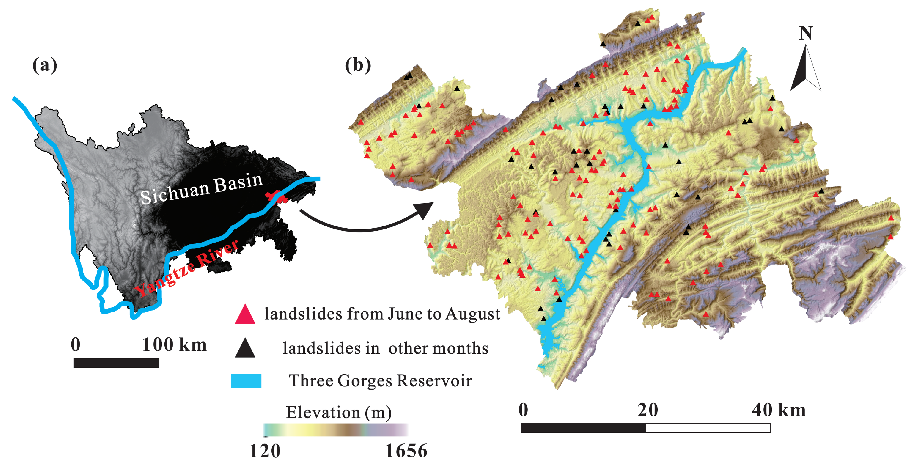
2. Study Area
3. Materials and Methods
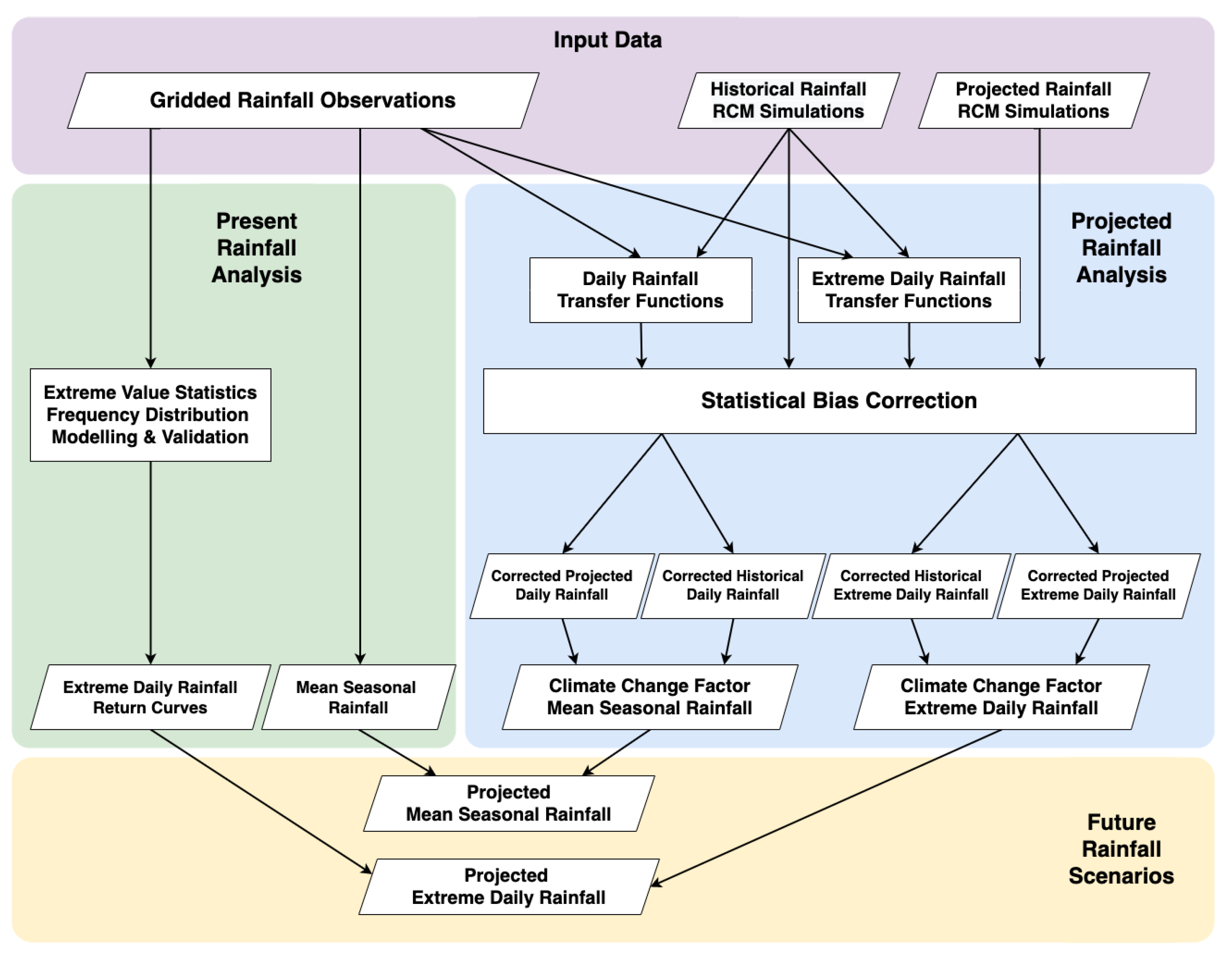
3.1. Methodological Framework
3.2. Input Data
3.3. Present Rainfall Analysis
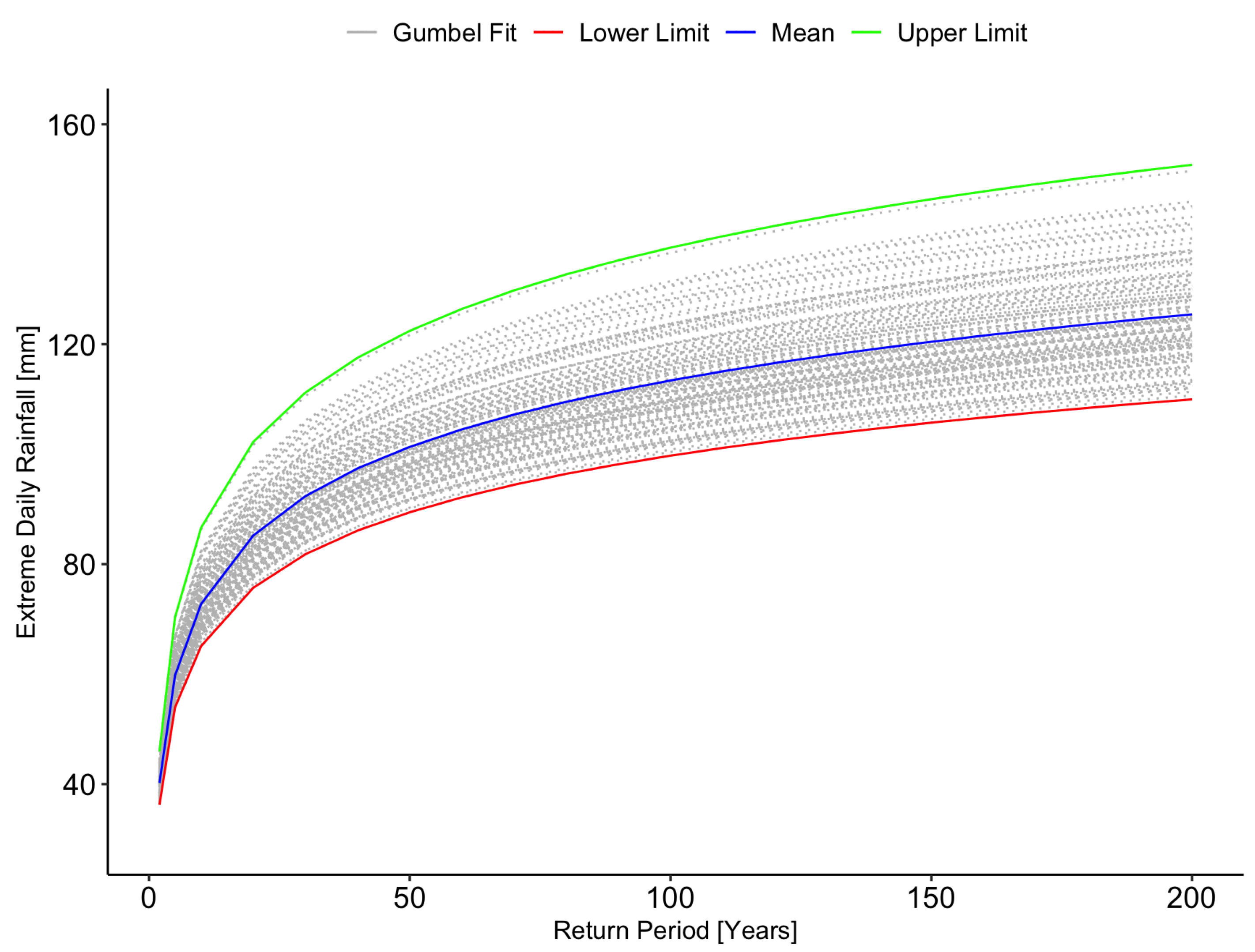
3.3.1. Extreme Daily Rainfall Analysis
3.3.2. Goodness-of-Fit Tests
3.4. Projected Rainfall Analysis
3.4.1. Quantile Delta Mapping Bias Correction
3.4.2. Multi-Model Ensemble Projections
4. Results
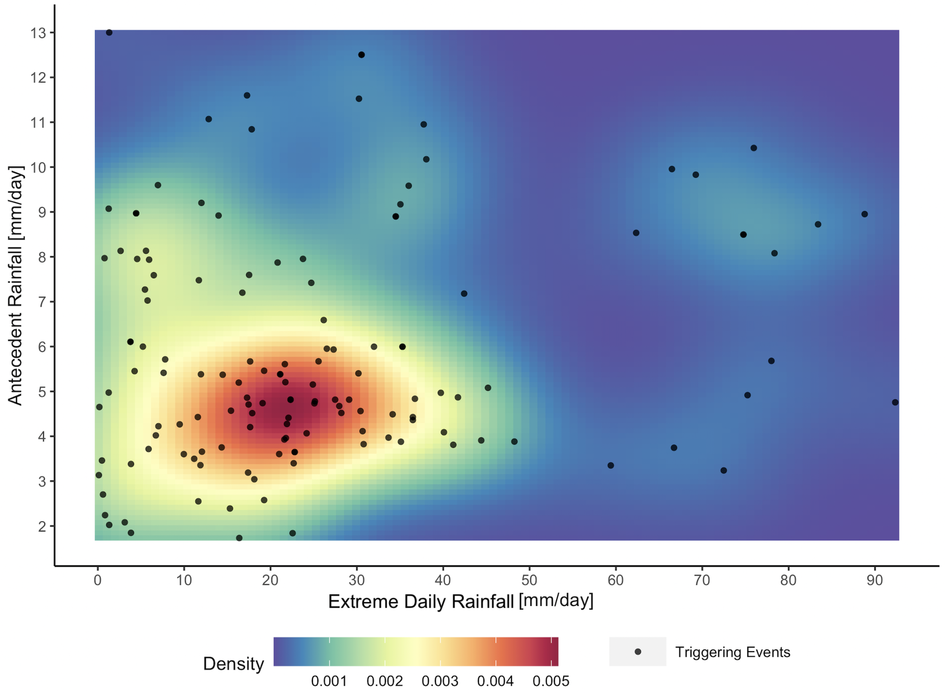
4.1. Reconstruction of Triggering Rainfall Conditions
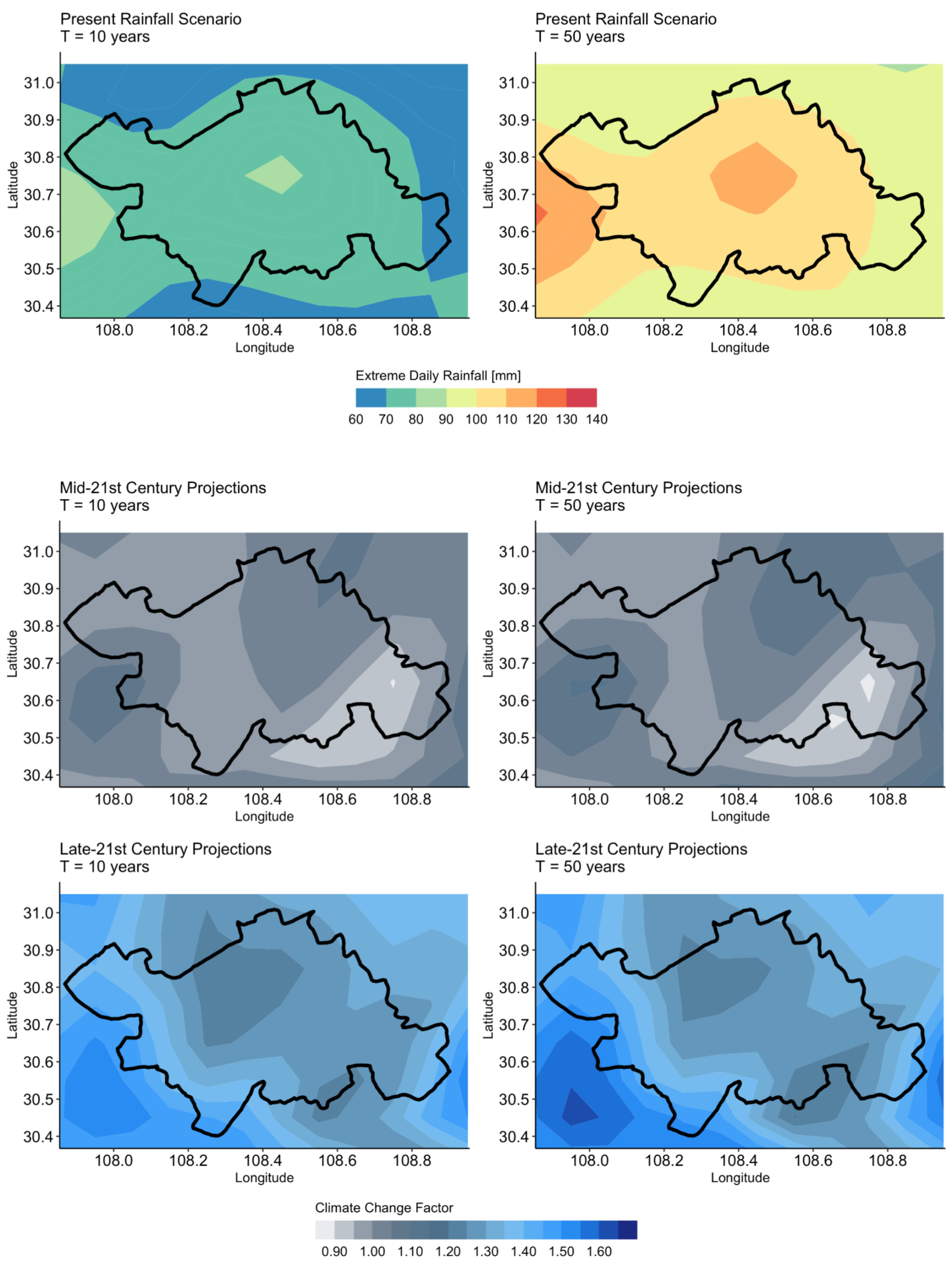
4.2. Extreme Daily Rainfall Scenarios
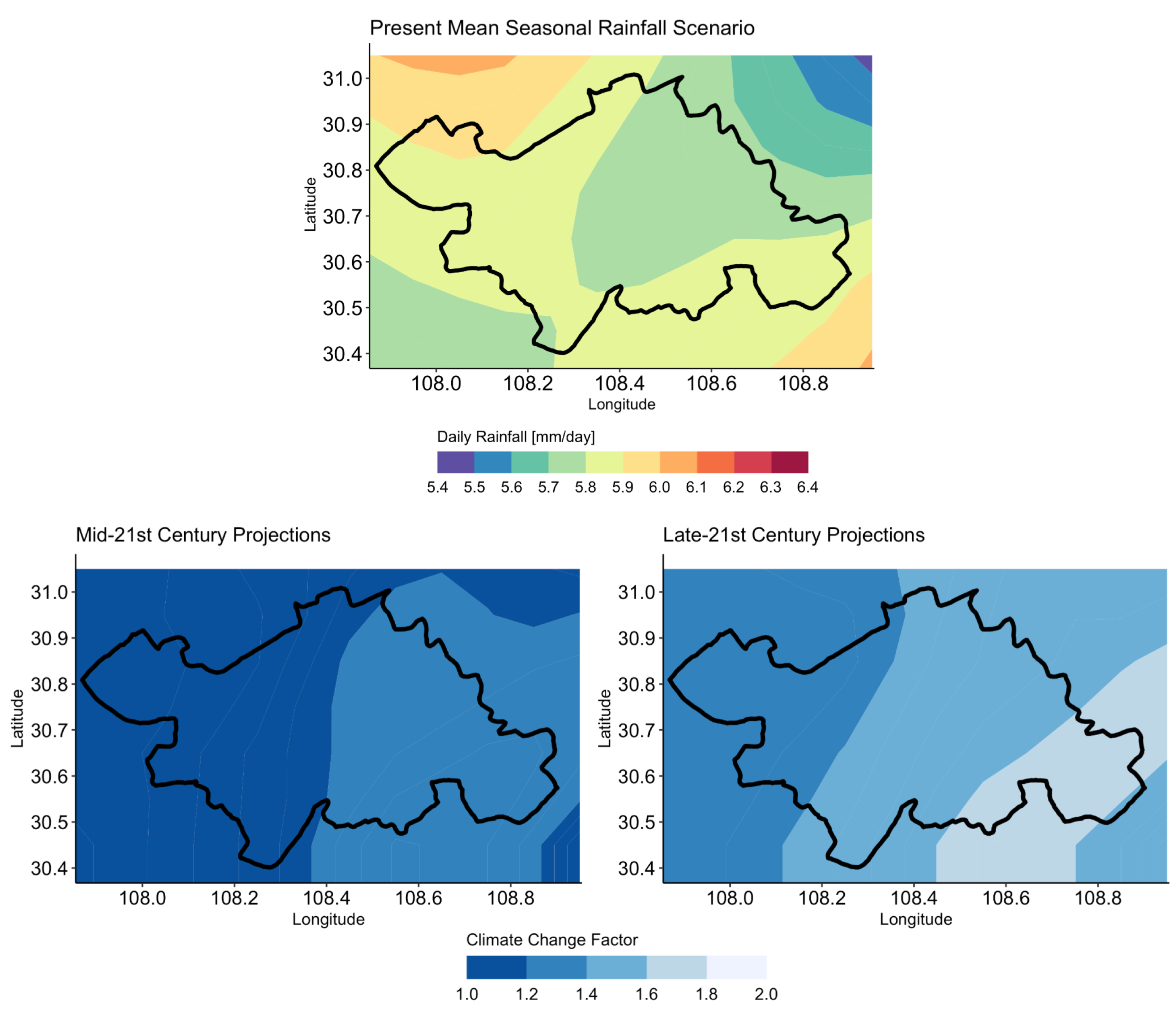
4.3. Mean Seasonal Rainfall Scenarios
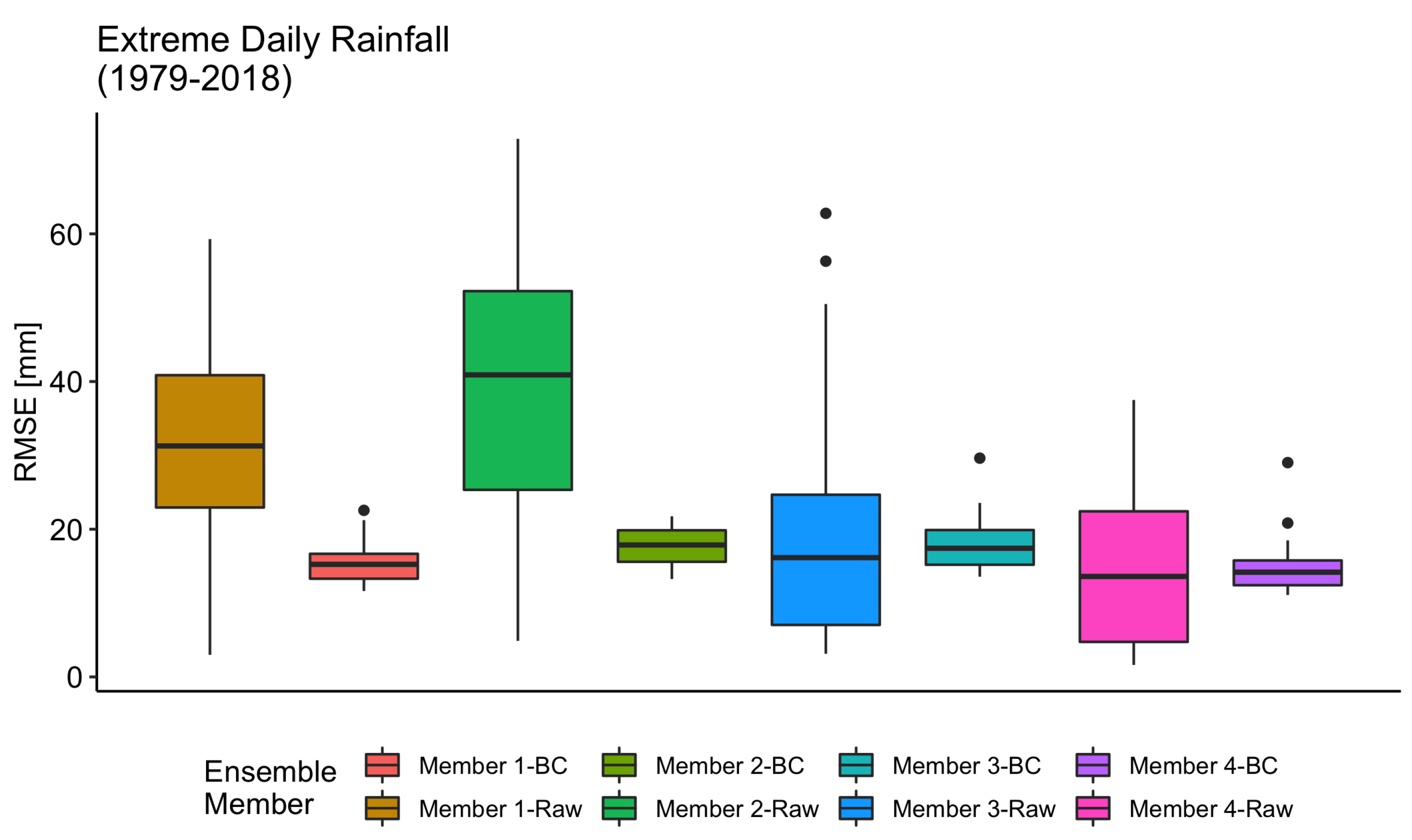
4.4. Bias Correction Performance
4.5. Uncertainty in the Ensemble Projections
5. Discussion
6. Conclusions
Author Contributions
Funding
Institutional Review Board Statement
Informed Consent Statement
Data Availability Statement
Acknowledgments
Conflicts of Interest
References
- Wallemacq, P.; House, R. Economic Losses, Poverty & Disasters: 1998–2017; Center for Research on the Epidemiology of Disasters (CRED) & United Nations Office for Disaster Risk Reduction (UNDRR): Geneva, Switzerland, 2018. [Google Scholar]
- Froude, M.J.; Petley, D.N. Global fatal landslide occurrence from 2004 to 2016. Nat. Hazards Earth Syst. Sci. 2018, 18, 2161–2181. [Google Scholar] [CrossRef] [Green Version]
- Gariano, S.L.; Guzzetti, F. Landslides in a changing climate. Earth-Sci. Rev. 2016, 162, 227–252. [Google Scholar] [CrossRef] [Green Version]
- Hartmann, D.L. Chapter 13—Anthropogenic Climate Change. In Global Physical Climatology, 2nd ed.; Hartmann, D.L., Ed.; Elsevier: Amsterdam, The Netherlands; pp. 397–425. [CrossRef]
- Keenan, R.; Reams, G.; Achard, F.; de Freitas, J.; Grainger, A.; Lindquist, E. Dynamics of global forest area: Results from the FAO Global Forest Resources Assessment 2015. For. Ecol. Manag. 2015, 352, 9–20. [Google Scholar] [CrossRef]
- Groisman, P.Y.; Knight, R.W.; Easterling, D.R.; Karl, T.R.; Hegerl, G.C.; Razuvaev, V.N. Trends in Intense Precipitation in the Climate Record. J. Clim. 2005, 18, 1326–1350. [Google Scholar] [CrossRef]
- Alexander, L.V.; Zhang, X.; Peterson, T.C.; Caesar, J.; Gleason, B.; Klein Tank, A.M.G.; Haylock, M.; Collins, D.; Trewin, B.; Rahimzadeh, F.; et al. Global observed changes in daily climate extremes of temperature and precipitation. J. Geophys. Res. Atmos. 2006, 111. [Google Scholar] [CrossRef] [Green Version]
- Medina, V.; Hürlimann, M.; Guo, Z.; Lloret, A.; Vaunat, J. Fast physically-based model for rainfall-induced landslide susceptibility assessment at regional scale. CATENA 2021, 201, 105213. [Google Scholar] [CrossRef]
- Scheidl, C.; Heiser, M.; Kamper, S.; Thaler, T.; Klebinder, K.; Nagl, F.; Lechner, V.; Markart, G.; Rammer, W.; Seidl, R. The influence of climate change and canopy disturbances on landslide susceptibility in headwater catchments. Sci. Total Environ. 2020, 742, 140588. [Google Scholar] [CrossRef]
- Crozier, M. Landslides: Causes, Consequences and Environment; Routledge: London, UK, 1986. [Google Scholar]
- Hong, M.; Kim, J.; Jeong, S. Rainfall intensity-duration thresholds for landslide prediction in South Korea by considering the effects of antecedent rainfall. Landslides 2018, 15, 523–534. [Google Scholar] [CrossRef]
- Khan, Y.A.; Lateh, H.; Baten, M.A.; Kamil, A.A. Critical antecedent rainfall conditions for shallow landslides in Chittagong City of Bangladesh. Environ. Earth Sci. 2012, 67, 97–106. [Google Scholar] [CrossRef]
- Kim, S.W.; Chun, K.W.; Kim, M.; Catani, F.; Choi, B.; Seo, J.I. Effect of antecedent rainfall conditions and their variations on shallow landslide-triggering rainfall thresholds in South Korea. Landslides 2021, 18, 569–582. [Google Scholar] [CrossRef]
- Ma, T.; Li, C.; Lu, Z.; Wang, B. An effective antecedent precipitation model derived from the power-law relationship between landslide occurrence and rainfall level. Geomorphology 2014, 216, 187–192. [Google Scholar] [CrossRef]
- Marques, R.; Zêzere, J.; Trigo, R.; Gaspar, J.; Trigo, I. Rainfall patterns and critical values associated with landslides in Povoação County (São Miguel Island, Azores): Relationships with the North Atlantic Oscillation. Hydrol. Process. 2008, 22, 478–494. [Google Scholar] [CrossRef]
- Mathew, J.; Babu, D.G.; Kundu, S.; Kumar, K.V.; Pant, C.C. Integrating intensity–duration-based rainfall threshold and antecedent rainfall-based probability estimate towards generating early warning for rainfall-induced landslides in parts of the Garhwal Himalaya, India. Landslides 2014, 11, 575–588. [Google Scholar] [CrossRef]
- Tang, D.; Li, D.Q.; Cao, Z.J. Slope stability analysis in the Three Gorges Reservoir Area considering effect of antecedent rainfall. Georisk Assess. Manag. Risk Eng. Syst. Geohazards 2017, 11, 161–172. [Google Scholar] [CrossRef]
- Tu, X.; Kwong, A.; Dai, F.; Tham, L.; Min, H. Field monitoring of rainfall infiltration in a loess slope and analysis of failure mechanism of rainfall-induced landslides. Eng. Geol. 2009, 105, 134–150. [Google Scholar] [CrossRef]
- Shou, K.J.; Yang, C.M. Predictive analysis of landslide susceptibility under climate change conditions—A study on the Chingshui River Watershed of Taiwan. Eng. Geol. 2015, 192, 46–62. [Google Scholar] [CrossRef]
- Lin, Q.; Wang, Y.; Glade, T.; Zhang, J.; Zhang, Y. Assessing the spatiotemporal impact of climate change on event rainfall characteristics influencing landslide occurrences based on multiple GCM projections in China. Clim. Chang. 2020, 162, 761–779. [Google Scholar] [CrossRef]
- Khalili, M.; Van Nguyen, V.T. An efficient statistical approach to multi-site downscaling of daily precipitation series in the context of climate change. Clim. Dyn. 2017, 49, 2261–2278. [Google Scholar] [CrossRef]
- Switzman, H.; Razavi, T.; Traore, S.; Coulibaly, P.; Burn, D.H.; Henderson, J.; Fausto, E.; Ness, R. Variability of Future Extreme Rainfall Statistics: Comparison of Multiple IDF Projections. J. Hydrol. Eng. 2017, 22, 04017046. [Google Scholar] [CrossRef]
- Padulano, R.; Reder, A.; Rianna, G. An ensemble approach for the analysis of extreme rainfall under climate change in Naples (Italy). Hydrol. Process. 2019, 33, 2020–2036. [Google Scholar] [CrossRef]
- Uzielli, M.; Rianna, G.; Ciervo, F.; Mercogliano, P.; Eidsvig, U.K. Temporal evolution of flow-like landslide hazard for a road infrastructure in the municipality of Nocera Inferiore (Southern Italy) under the effect of climate change. Nat. Hazards Earth Syst. Sci. 2018, 18, 3019–3035. [Google Scholar] [CrossRef] [Green Version]
- Hürlimann, M.; Guo, Z.; Puig-Polo, C.; Medina, V. Impacts of future climate and land cover changes on landslide susceptibility: Regional scale modelling in the Val d’Aran region (Pyrenees, Spain). Landslides 2022, 19, 99–118. [Google Scholar] [CrossRef]
- Rianna, G.; Reder, A.; Mercogliano, P.; Pagano, L. Evaluation of Variations in Frequency of Landslide Events Affecting Pyroclastic Covers in Campania Region under the Effect of Climate Changes. Hydrology 2017, 4, 34. [Google Scholar] [CrossRef] [Green Version]
- Alvioli, M.; Melillo, M.; Guzzetti, F.; Rossi, M.; Palazzi, E.; von Hardenberg, J.; Brunetti, M.T.; Peruccacci, S. Implications of climate change on landslide hazard in Central Italy. Sci. Total Environ. 2018, 630, 1528–1543. [Google Scholar] [CrossRef]
- Bordoni, M.; Corradini, B.; Lucchelli, L.; Valentino, R.; Bittelli, M.; Vivaldi, V.; Meisina, C. Empirical and Physically Based Thresholds for the Occurrence of Shallow Landslides in a Prone Area of Northern Italian Apennines. Water 2019, 11, 2653. [Google Scholar] [CrossRef] [Green Version]
- Segoni, S.; Piciullo, L.; Gariano, S.L. A review of the recent literature on rainfall thresholds for landslide occurrence. Landslides 2018, 15, 1483–1501. [Google Scholar] [CrossRef]
- Bordoni, M.; Inzaghi, F.; Vivaldi, V.; Valentino, R.; Bittelli, M.; Meisina, C. A Data-Driven Method for the Temporal Estimation of Soil Water Potential and Its Application for Shallow Landslides Prediction. Water 2021, 13, 1208. [Google Scholar] [CrossRef]
- Huang, Y.; Xiao, W.; Hou, B.; Zhou, Y.; Hou, G.; Yi, L.; Cui, H. Hydrological projections in the upper reaches of the Yangtze River Basin from 2020 to 2050. Sci. Rep. 2021, 11, 9720. [Google Scholar] [CrossRef]
- Peres, D.J.; Cancelliere, A. Modeling impacts of climate change on return period of landslide triggering. J. Hydrol. 2018, 567, 420–434. [Google Scholar] [CrossRef]
- Dahal, R.K.; Hasegawa, S. Representative rainfall thresholds for landslides in the Nepal Himalaya. Geomorphology 2008, 100, 429–443. [Google Scholar] [CrossRef]
- Giorgi, F.; Coppola, E. Does the model regional bias affect the projected regional climate change? An analysis of global model projections. Clim. Chang. 2010, 100, 787–795. [Google Scholar] [CrossRef]
- Christensen, J.H.; Kjellström, E.; Giorgi, F.; Lenderink, G.; Rummukainen, M. Weight assignment in regional climate models. Clim. Res. 2010, 44, 179–194. [Google Scholar] [CrossRef]
- Huang, F.; Yin, K.; Huang, J.; Gui, L.; Wang, P. Landslide susceptibility mapping based on self-organizing-map network and extreme learning machine. Eng. Geol. 2017, 223, 11–22. [Google Scholar] [CrossRef]
- Guo, Z.; Yin, K.; Huang, F.; Fu, S.; Zhang, W. Evaluation of landslide susceptibility based on landslide classification and weighted frequency ratio model. Chin. J. Rock Mech. Eng. 2019, 38, 287–300. [Google Scholar] [CrossRef]
- Xiao, T.; Segoni, S.; Chen, L.; Yin, K.; Casagli, N. A step beyond landslide susceptibility maps: A simple method to investigate and explain the different outcomes obtained by different approaches. Landslides 2020, 17, 627–640. [Google Scholar] [CrossRef] [Green Version]
- Gui, L.; Yin, K.; Glade, T. Landslide displacement analysis based on fractal theory, in Wanzhou District, Three Gorges Reservoir, China. Geomat. Nat. Hazards Risk 2016, 7, 1707–1725. [Google Scholar] [CrossRef] [Green Version]
- Huang, C.; Zhou, Q.; Zhou, L.; Cao, Y. Ancient landslide in Wanzhou District analysis from 2015 to 2018 based on ALOS-2 data by QPS-InSAR. Nat. Hazards 2021, 109, 1777–1800. [Google Scholar] [CrossRef]
- Petley, D.N. Landslide disaster mitigation in the Three Gorges Reservoir, China. Mt. Res. Dev. 2010, 30, 184–185. [Google Scholar] [CrossRef]
- Liu, Y.; Yin, K.; Chen, L.; Wang, W.; Liu, Y. A community-based disaster risk reduction system in Wanzhou, China. Int. J. Disaster Risk Reduct. 2016, 19, 379–389. [Google Scholar] [CrossRef]
- Xiao, T.; Yin, K.; Yao, T.; Liu, S. Spatial prediction of landslide susceptibility using GIS-based statistical and machine learning models in Wanzhou County, Three Gorges Reservoir, China. Acta Geochim. 2019, 38, 654–669. [Google Scholar] [CrossRef]
- Song, Y.; Niu, R.; Xu, S.; Ye, R.; Peng, L.; Guo, T.; Li, S.; Chen, T. Landslide Susceptibility Mapping Based on Weighted Gradient Boosting Decision Tree in Wanzhou Section of the Three Gorges Reservoir Area (China). ISPRS Int. J. Geo-Inf. 2019, 8, 4. [Google Scholar] [CrossRef] [Green Version]
- Xiao, L.; Wang, J.; Zhu, Y.; Zhang, J. Quantitative Risk Analysis of a Rainfall-Induced Complex Landslide in Wanzhou County, Three Gorges Reservoir, China. Int. J. Disaster Risk Sci. 2020, 11, 347–363. [Google Scholar] [CrossRef] [Green Version]
- Chinese Academy of Sciences. Resource and Environment Science and Data Center. 2021. Available online: http://www.resdc.cn/ (accessed on 20 November 2021).
- IUSS Working Group WRB. World reference base for soil resources 2014. International soil classification system for naming soils and creating legends for soil maps. World Soil Resources Reports No. 106. Exp. Agric. 2007, 43, 264. [Google Scholar] [CrossRef]
- Gu, H.; Yu, Z.; Yang, C.; Ju, Q. Projected Changes in Hydrological Extremes in the Yangtze River Basin with an Ensemble of Regional Climate Simulations. Water 2018, 10, 1279. [Google Scholar] [CrossRef] [Green Version]
- Freychet, N.; Hsu, H.H.; Chou, C.; Wu, C.H. Asian Summer Monsoon in CMIP5 Projections: A Link between the Change in Extreme Precipitation and Monsoon Dynamics. J. Clim. 2015, 28, 1477–1493. [Google Scholar] [CrossRef]
- Xu, Y.; Gao, X.; Giorgi, F.; Zhou, B.; Shi, Y.; Wu, J.; Zhang, Y. Projected Changes in Temperature and Precipitation Extremes over China as Measured by 50-yr Return Values and Periods Based on a CMIP5 Ensemble. Adv. Atmos. Sci. 2018, 35, 376–388. [Google Scholar] [CrossRef]
- Qin, P.; Xie, Z.; Zou, J.; Liu, S.; Chen, S. Future Precipitation Extremes in China under Climate Change and Their Physical Quantification Based on a Regional Climate Model and CMIP5 Model Simulations. Adv. Atmos. Sci. 2021, 38, 460–479. [Google Scholar] [CrossRef]
- He, J.; Yang, K.; Tang, W.; Lu, H.; Qin, J.; Chen, Y.; Li, X. The first high-resolution meteorological forcing dataset for land process studies over China. Sci. Data 2020, 7, 25. [Google Scholar] [CrossRef] [Green Version]
- Taylor, K.E.; Stouffer, R.J.; Meehl, G.A. An Overview of CMIP5 and the Experiment Design. Bull. Am. Meteorol. Soc. 2012, 93, 485–498. [Google Scholar] [CrossRef] [Green Version]
- Kim, G.; Cha, D.H.; Park, C.; Jin, C.S.; Lee, D.K.; Suh, M.S.; Oh, S.G.; Hong, S.Y.; Ahn, J.B.; Min, S.K.; et al. Evaluation and Projection of Regional Climate over East Asia in CORDEX-East Asia Phase I Experiment. Asia-Pac. J. Atmos. Sci. 2021, 57, 119–134. [Google Scholar] [CrossRef]
- Giorgi, F.; Diffenbaugh, N.S.; Gao, X.J.; Coppola, E.; Dash, S.K.; Frumento, O.; Rauscher, S.A.; Remedio, A.; Sanda, I.S.; Steiner, A.; et al. The Regional Climate Change Hyper-Matrix Framework. Eos Trans. Am. Geophys. Union 2008, 89, 445–446. [Google Scholar] [CrossRef]
- Jacob, D.; Elizalde, A.; Haensler, A.; Hagemann, S.; Kumar, P.; Podzun, R.; Rechid, D.; Remedio, A.R.; Saeed, F.; Sieck, K.; et al. Assessing the Transferability of the Regional Climate Model REMO to Different COordinated Regional Climate Downscaling EXperiment (CORDEX) Regions. Atmosphere 2012, 3, 181–199. [Google Scholar] [CrossRef] [Green Version]
- Giorgi, F.; Coppola, E.; Solmon, F.; Mariotti, L.; Sylla, M.B.; Bi, X.; Elguindi, N.; Diro, G.T.; Nair, V.; Giuliani, G.; et al. RegCM4: Model description and preliminary tests over multiple CORDEX domains. Clim. Res. 2012, 52, 7–29. [Google Scholar] [CrossRef] [Green Version]
- Gao, X.; Shi, Y.; Han, Z.; Wang, M.; Wu, J.; Zhang, D.; Xu, Y.; Giorgi, F. Performance of RegCM4 over major river basins in China. Adv. Atmos. Sci. 2017, 34, 441–455. [Google Scholar] [CrossRef]
- Jingwei, X.; Min, X.; Jiang, X.; Remedio, A.; Sein, D.; Koldunov, N.; Jacob, D. The Assessment of Surface Air Temperature and Precipitation Simulated by Regional Climate Model REMO over China. Clim. Chang. Res. 2016, 12, 286–293. [Google Scholar]
- Jones, C.D.; Hughes, J.K.; Bellouin, N.; Hardiman, S.C.; Jones, G.S.; Knight, J.; Liddicoat, S.; O’Connor, F.M.; Andres, R.J.; Bell, C.; et al. The HadGEM2-ES implementation of CMIP5 centennial simulations. Geosci. Model Dev. 2011, 4, 543–570. [Google Scholar] [CrossRef] [Green Version]
- Ilyina, T.; Six, K.D.; Segschneider, J.; Maier-Reimer, E.; Li, H.; Núñez-Riboni, I. Global ocean biogeochemistry model HAMOCC: Model architecture and performance as component of the MPI-Earth system model in different CMIP5 experimental realizations. J. Adv. Model. Earth Syst. 2013, 5, 287–315. [Google Scholar] [CrossRef]
- Coles, S. An Introduction to Statistical Modeling of Extreme Values; Springer Series in Statistics; Springer: London, UK, 2001. [Google Scholar] [CrossRef]
- Fischer, M.; Rust, H.W.; Ulbrich, U. Seasonal Cycle in German Daily Precipitation Extremes. Meteorol. Z. 2018, 27, 3–13. [Google Scholar] [CrossRef]
- Rust, H.W.; Maraun, D.; Osborn, T.J. Modelling seasonality in extreme precipitation. Eur. Phys. J. Spec. Top. 2009, 174, 99–111. [Google Scholar] [CrossRef]
- Delignette-Muller, M.L.; Dutang, C. fitdistrplus: An R Package for Fitting Distributions. J. Stat. Softw. 2015, 64, 1–34. [Google Scholar] [CrossRef] [Green Version]
- Laio, F. Cramer–von Mises and Anderson-Darling goodness of fit tests for extreme value distributions with unknown parameters. Water Resour. Res. 2004, 40. [Google Scholar] [CrossRef]
- Marsaglia, G.; Marsaglia, J. Evaluating the Anderson-Darling Distribution. J. Stat. Softw. 2004, 9, 1–5. [Google Scholar] [CrossRef] [Green Version]
- Cannon, A.J.; Sobie, S.R.; Murdock, T.Q. Bias Correction of GCM Precipitation by Quantile Mapping: How Well Do Methods Preserve Changes in Quantiles and Extremes? J. Clim. 2015, 28, 6938–6959. [Google Scholar] [CrossRef]
- Tong, Y.; Gao, X.; Han, Z.; Xu, Y.; Xu, Y.; Giorgi, F. Bias correction of temperature and precipitation over China for RCM simulations using the QM and QDM methods. Clim. Dyn. 2021, 57, 1425–1443. [Google Scholar] [CrossRef]
- Xu, L.; Wang, A. Application of the Bias Correction and Spatial Downscaling Algorithm on the Temperature Extremes From CMIP5 Multimodel Ensembles in China. Earth Space Sci. 2019, 6, 2508–2524. [Google Scholar] [CrossRef] [Green Version]
- Maraun, D. Bias Correcting Climate Change Simulations—A Critical Review. Curr. Clim. Chang. Rep. 2016, 2, 211–220. [Google Scholar] [CrossRef] [Green Version]
- Kim, S.; Shin, J.Y.; Ahn, H.; Heo, J.H. Selecting Climate Models to Determine Future Extreme Rainfall Quantiles. J. Korean Soc. Hazard Mitig. 2019, 19, 55–69. [Google Scholar] [CrossRef]
- Durman, C.F.; Gregory, J.M.; Hassell, D.C.; Jones, R.G.; Murphy, J.M. A comparison of extreme European daily precipitation simulated by a global and a regional climate model for present and future climates. Q. J. R. Meteorol. Soc. 2001, 127, 1005–1015. [Google Scholar] [CrossRef]
- Akima, H. Algorithm 760: Rectangular-grid-data surface fitting that has the accuracy of a bicubic polynomial. ACM Trans. Math. Softw. 1996, 22, 357–361. [Google Scholar] [CrossRef]
- Ferrer, J.V.C. A Regional Assessment on the Influence of Climate Change on Summer Rainfall: An Application to Shallow Landsliding in Wanzhou County, China. Master’s Thesis, UPC BarcelonaTECH, Barcelona, Spain, 2021. [Google Scholar]
- Ozturk, U.; Saito, H.; Matsushi, Y.; Crisologo, I.; Schwanghart, W. Can global rainfall estimates (satellite and reanalysis) aid landslide hindcasting? Landslides 2021, 18, 3119–3133. [Google Scholar] [CrossRef]
- Kim, S.; Joo, K.; Kim, H.; Shin, J.Y.; Heo, J.H. Regional quantile delta mapping method using regional frequency analysis for regional climate model precipitation. J. Hydrol. 2021, 596, 125685. [Google Scholar] [CrossRef]
- Nguyen, H.; Mehrotra, R.; Sharma, A. Can the variability in precipitation simulations across GCMs be reduced through sensible bias correction? Clim. Dyn. 2017, 49, 3257–3275. [Google Scholar] [CrossRef]
- He, Q.; Yang, J.; Chen, H.; Liu, J.; Ji, Q.; Wang, Y.; Tang, F. Evaluation of Extreme Precipitation Based on Three Long-Term Gridded Products over the Qinghai-Tibet Plateau. Remote Sens. 2021, 13, 3010. [Google Scholar] [CrossRef]
- Yang, Y.; Tang, J.; Xiong, Z.; Wang, S.; Yuan, J. An intercomparison of multiple statistical downscaling methods for daily precipitation and temperature over China: Present climate evaluations. Clim. Dyn. 2019, 53, 4629–4649. [Google Scholar] [CrossRef]
- Crozier, M.J. Deciphering the effect of climate change on landslide activity: A review. Geomorphology 2010, 124, 260–267. [Google Scholar] [CrossRef]
- Koutsoyiannis, D. Statistics of extremes and estimation of extreme rainfall: I. Theoretical investigation. Hydrol. Sci. J. 2004, 49, 3. [Google Scholar] [CrossRef] [Green Version]
- Yang, X.; Yu, X.; Wang, Y.; He, X.; Pan, M.; Zhang, M.; Liu, Y.; Ren, L.; Sheffield, J. The Optimal Multimodel Ensemble of Bias-Corrected CMIP5 Climate Models over China. J. Hydrometeorol. 2020, 21, 845–863. [Google Scholar] [CrossRef]
- Olmos Giménez, P.; García Galiano, S.G.; Giraldo-Osorio, J.D. Identifying a robust method to build RCMs ensemble as climate forcing for hydrological impact models. Atmos. Res. 2016, 174–175, 31–40. [Google Scholar] [CrossRef]


| Ensemble Members | GCM Model | RCM Model |
|---|---|---|
| Member 1 | HadGEM2-ES | REMO2015 |
| Member 2 | HadGEM2-ES | RegCM4 |
| Member 3 | MPI-ESM-LR | REMO2015 |
| Member 4 | MPI-ESM-MR | RegCM4 |
| Scenario | Period (Years) | RCM Scenario Outputs |
|---|---|---|
| Reference | 1979–2018 | Historical + RCP 8.5 |
| Mid-21st Century | 2021–2060 | RCP 8.5 |
| Late-21st Century | 2061–2100 | RCP 8.5 |
| Gumbel Fit Parameters | Minimum | Mean | Maximum |
|---|---|---|---|
| Scale | 14.6 | 17.3 | 21.7 |
| Beta | 29.4 | 32.9 | 36.9 |
| Mean | 30.3 | 33.9 | 38.1 |
| Standard Deviation | 18.8 | 22.2 | 27.8 |
| Goodness-of-Fit Test | Minimum | Mean | Maximum |
|---|---|---|---|
| KS Test | 0.029 | 0.052 | 0.082 |
| AD Test | 0.145 | 0.318 | 0.730 |
| CVM Test | 0.015 | 0.046 | 0.136 |
| Ensemble Members | Minimum | Mean | Maximum |
|---|---|---|---|
| Member 1 | 14.30 | 15.73 | 17.77 |
| Member 2 | 14.37 | 15.79 | 17.32 |
| Member 3 | 14.45 | 15.93 | 17.89 |
| Member 4 | 14.33 | 15.75 | 17.26 |
| Mid-21st Century | Late-21st Century | |
|---|---|---|
| Climate Change Factors | ||
| Extreme Daily Rainfall | 0.9–1.0 | 1.2–1.6 |
| Mean Seasonal Rainfall | 1.0–1.4 | 1.2–1.8 |
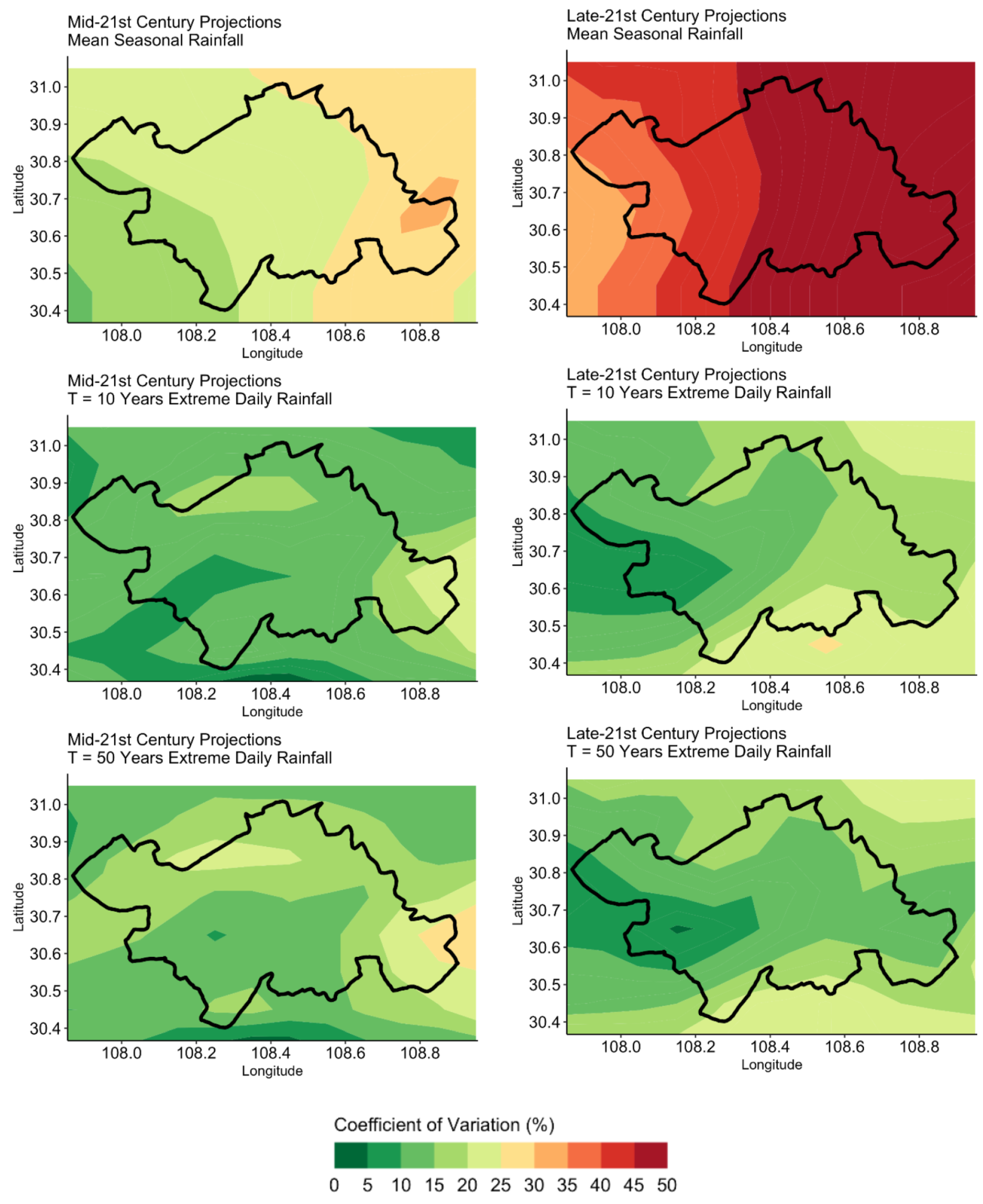
| Coefficients of Variation | ||
| Extreme Daily Rainfall | 5–25% | 5–25% |
| Mean Seasonal Rainfall | 10–35% | 30–50% |
Publisher’s Note: MDPI stays neutral with regard to jurisdictional claims in published maps and institutional affiliations. |
© 2022 by the authors. Licensee MDPI, Basel, Switzerland. This article is an open access article distributed under the terms and conditions of the Creative Commons Attribution (CC BY) license (https://creativecommons.org/licenses/by/4.0/).
Share and Cite
Ferrer, J.; Guo, Z.; Medina, V.; Puig-Polo, C.; Hürlimann, M. A Framework to Project Future Rainfall Scenarios: An Application to Shallow Landslide-Triggering Summer Rainfall in Wanzhou County China. Water 2022, 14, 873. https://doi.org/10.3390/w14060873
Ferrer J, Guo Z, Medina V, Puig-Polo C, Hürlimann M. A Framework to Project Future Rainfall Scenarios: An Application to Shallow Landslide-Triggering Summer Rainfall in Wanzhou County China. Water. 2022; 14(6):873. https://doi.org/10.3390/w14060873
Chicago/Turabian StyleFerrer, Joaquin, Zizheng Guo, Vicente Medina, Càrol Puig-Polo, and Marcel Hürlimann. 2022. "A Framework to Project Future Rainfall Scenarios: An Application to Shallow Landslide-Triggering Summer Rainfall in Wanzhou County China" Water 14, no. 6: 873. https://doi.org/10.3390/w14060873
APA StyleFerrer, J., Guo, Z., Medina, V., Puig-Polo, C., & Hürlimann, M. (2022). A Framework to Project Future Rainfall Scenarios: An Application to Shallow Landslide-Triggering Summer Rainfall in Wanzhou County China. Water, 14(6), 873. https://doi.org/10.3390/w14060873