Abstract
The sustainable management of water resources, whether surface or underground, requires the identification of the flows involved and the possibility of achieving the water balance of the water resource. These require knowledge of the main flow components with a sufficient level of accuracy. Hydrological simulation models are valuable tools for studying flow at the watershed scale but rely on data that are rarely available; therefore, they require the implementation of field investigations. There is thus a need for simple and practical tools for studying the functioning of a watershed and identifying the different components of the flows. In this paper, a method that uses only weather data, volumes of water abstraction by pumping or diversion, and flows measured at the outlet is proposed. The use of cumulative multi-year curves of measured flows or rainfall provides an assessment of the unknown flows that can take place in the watershed, as well as the order of the respective magnitudes of fast and slow flows. Its application to 20 French Mediterranean watersheds shows that it is possible to properly estimate the order of magnitude of losses or gains linked to karst flows and irrigation input. External inflows or outflows can represent up to 150% of the flow measured at the outlet. The annual volumes estimated by using this method are indeed very close (R2 = 93%) to those provided by existing knowledge. The proposed method can constitute a first approach for the quantification of flows and help to guide the implementation of field investigations and more sophisticated approaches such as hydrological modelling.
1. Introduction
1.1. Background
The sustainable management of water resources, whether surface or underground, requires the identification of the flows involved and the possibility of achieving a water balance at the scale of the water resource needing to be managed. Establishing the water balance requires knowledge of the different components of the flows [1]. While technologies used for measuring water balance components continue to improve, all components of the water balance have substantial uncertainty at the watershed scale [2]. The main components taken into account are rainfall, evapotranspiration, water abstractions from surficial or ground water by pumping and diversion, and flows measured at the outlet of the watershed. In many cases, the water balance is not equilibrated. This can be due to other components of the water balance that are often neglected but can become very important when the time scale of the balance calculation is small. They include interception by vegetation, depression storage, soil storage, and groundwater storage. For larger time scales, the total variation in these flow components evens out and becomes negligible. In other cases, the water balance mismatch could be related to the existence of water exchanges with water resources outside of the topographic watershed. Such exchanges may correspond to karst networks allowing the transfer of water from one watershed to another, to deep underground flows occurring at regional scales, or to water transfer used for irrigation.
The assessment of the water balance and the calibration of a hydrological model require knowledge of the flows leaving the watershed. These flows are generally measured at the outlet of the watershed by setting up a hydrometric gauging station. In some watersheds, gauging stations provide flow measurements that are not compatible with their size and the rain that falls there. Unfortunately, the flow components and structures responsible for this difference between the expected flows and those actually observed are not always known [3,4,5]. It is therefore sometimes impossible to quantify the flows and study the functioning of the watershed.
Catchments, generally understood as the drainage areas of low-order streams, are often regarded as closed hydrologic entities but can be leaky due to groundwater outflow or inflow across topographic divides [6]. Actual flows may include a net input of groundwater that originates outside the surface watershed boundaries or a net output of groundwater below the surface watershed boundaries [2]. In crystalline basement terrains, topographic watersheds and hydrogeological basins are generally close. In alluvium and carbonate domains, surface and underground flows may be disjointed [7]. This may be related to a topography that is independent of the geology. This may also be due to a dip in the geological layers directed towards the boundaries of the topographic basin [6]. This can still be linked to the presence of interbasin karst networks bypassing the watershed limits [8]. Such geological features can allow the entry or the exit of water across the watershed boundaries [9,10], making it more difficult to carry out a hydrological balance assessment [11].
1.2. Recent Developments
Numerous studies have shown that uncertainties in key aspects of the system create limitations in water resource management [12]. A great deal of work has been carried out on the use of hydrographs for baseflow assessment and aquifer recharge [13,14,15]. These approaches classically use a flow hydrograph and study its dependence on rainfall. They perform work on hydrograph lengths (i.e., time periods) centered on a rain event or season. This makes it possible to study the reactivity of flows to rainfall events, but does not always take into account the very slow components of flows. Other studies focus on the exchange between surface and groundwater by studying the evolution of flow along the stream [8,16,17]. However, such approaches require significant field investigations both in terms of time (several years of monitoring) and space (serial gauging along the entire river).
Hydrological simulation models are valuable tools for studying flow at the watershed scale. Great progress has been made in recent decades with regard to simulating flows in watersheds [18,19]. Numerous models, such as SWAT, MIKE-SHE, HBV, TOPMODEL, and VIC [20], exist, allowing the different components of the flow to be taken into account in a more or less faithful and relevant way. However, the implementation of these models requires, at least, the knowledge of the rain falling on the watershed and the water discharge at its outlet. There are many difficulties in implementing and calibrating a hydrological model, such as the availability of data, multiple reservoirs, elevation and slopes in mountainous regions, the representation of channels, irrigation return flows, vegetative cover, and water abstractions from surficial and ground water [21]. Surface water and groundwater are often regarded and studied as two separate systems [22] and not always considered at the same time in simulation models. In many cases, models can only sufficiently simulate what is already known [23]. For these reasons, various works have attempted to propose simple and easy-to-apply methods to estimate some components of watershed hydrology [24,25,26].
1.3. Objectives of the Work
The assessment of the water balance is often difficult because of its geological, hydrological, and climatic complexity. On the other hand, hydrological models that can assist in calculating the water balance at the watershed scale are difficult to implement and require data that are not readily available. In many cases, the level of effort and cost involved are not justified in view of the needs and the financial means available. It is therefore necessary in this case to use methods that are less detailed and precise than what models can provide but that can be quickly applied with the only information that is usually available. Such a simple and practical method based on usually available knowledge has not yet been reported in the literature.
The objective of this work was therefore to propose a simple and robust method for assessing the global functioning of a watershed and quickly identifying the unknown components of the water balance. This method is intended to be a simple and rapid diagnostic approach to the global functioning of the water resources at the watershed scale and not a method for the fine analysis of the flow dynamics, as simulation models can claim to be. This method does not pretend to provide a detailed assessment of the hydrology of the watershed, but it is able to quickly identify its different components. This method should be easy to implement on watersheds where the only knowledge available is weather data, water abstractions from surficial and ground water by pumping and diversion, and observed flows at the watershed outlet.
2. Materials and Methods
2.1. Data Used for the Diagnostic Method
In watersheds based on porous media or carbonate terrains, the underground part of the flows can often be important, even dominant. However, the direct measurement of groundwater flow is impossible. The only possible evaluation is that offered by mathematical modeling. Unfortunately, such modeling requires data on the parameters and forcing conditions that control the flow. On the other hand, information is available on the rainfall occurring in many watersheds and on the flow rates at their outlet. We propose an approach that uses this information to assess the unknown portion of groundwater flow related to exchanges with outside the watershed.
In this paper, the word “watershed” is used in its etymological, topographic sense where “shed” means “ridge of high ground between two valleys or lower ground” [27]. In this sense, the word “watershed” is synonymous with “surface water catchment” [28]. The topographic watershed thus differs from the total water catchment, which includes both surface and groundwater catchments. In Mediterranean watersheds where karstic flows are common, subsurface transfers between watersheds are often observed (e.g., [29,30]). However, it is often very difficult, if not impossible, to determine the area of land contributing to these water exchanges. This often requires the implementation of heavier field investigations or modeling. For example, the authors of [31] couple tracing test techniques and semi-distributed hydrological modeling (SWAT) to solve the problem of the inconsistency between the topographical drainage divides and actual catchment boundaries in karst areas.
Figure 1 shows the different components considered in the proposed approach.
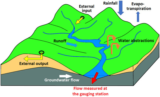
Figure 1.
Schematic diagram of the flow components taken into account in this method.
The water flow velocities at the soil surface, in subsurface layers, and deep in the aquifer are very different. They can vary from a few days to several years. It is therefore not possible to carry out a water balance assessment over a short period of time. The proposed approach was developed based on the use of several years of data. In this way, the flow time and temporal variability are no longer constraints for the calculation of the water budget. The different components of the flow are not calculated separately, thus eliminating sources of uncertainty and error. A one-decade calculation seems to be a good compromise to integrate the interannual hydro-climatic variability without being significantly affected by a change in land and water resource use.
In the proposed approach, components such as interception, depression storage, soil storage, groundwater storage, etc., are not taken into account, since the water balance is calculated over several years. On this time scale, variations due to these components are compensated for over time or their result becomes negligible. Over shorter periods of time, these elements must, of course, be taken into account, as they could represent a significant fraction of the water balance.
The unknown components of flow refer to subsurface inputs coming from outside the topographic watershed and to subsurface water flowing outside the topographic watershed that cannot be observed at the gauging station located at its topographic outlet. For example, the authors of [8] note that differences between measured and expected flow suggest large, unidentified inputs of groundwater.
This method takes into account rainfall, evapotranspiration, and water abstractions that refer to the pumping or diversion of surficial and ground water for drinking water, irrigation, and industry. The volumes withdrawn from water resources are known through declarations made by users to state services. The data are available on the internet on a yearly basis [32].
The weather data used came from the meteorological stations of the National or Local Weather Services [33]. The water abstractions were acquired through the compulsory declarations made to water agencies. Data were used to calculate the effective rainfall (or effective precipitation)—that is, the portion of rainfall available for runoff and groundwater recharge. The following calculation was conducted at each time step:
Effective Precipitation = Precipitation − Evapotranspiration − Variation in Soil Water Content
To perform this calculation, it is necessary to have the required data at regular time steps. We opted for a decadal time step (about 10 days). Each month was divided into three decades, with 10 days for the first two decades and the remaining number of days for the third. The decadal duration was compatible with the average duration of rainy periods, the transfer of water through the soil, the persistence of surface puddles, and the resistance of plants to water shortages. The use of a larger time step (e.g., one month) would smooth out rain and drought events too much (minimizing runoff and recharge), while a shorter time step (e.g., a day) would limit evapotranspiration and generally overestimate runoff and recharge.
The variation in the soil water content is controlled by the soil properties and the extractable soil water. This information is available in a cartographic form in different internet databases [34]. During a rain event, the amount of water that can enter the soil is a function of the available space in the soil, i.e., the difference between the total soil porosity and the water content already in the soil. Water that cannot enter the soil is available for runoff. In this hydro-pedological approach, Hortonian runoff (which occurs at the soil surface) is therefore calculated as the part of water that cannot infiltrate into the soil and that is not from an arbitrary runoff coefficient. Soil water content can be mobilized for evapotranspiration up to a minimum value corresponding to the inferior limit of available water (wilting point).
Subsequently, the water abstractions carried out using the pumping and diversion of surficial and ground water in the watershed were taken into account to calculate the net volume of flow. This net volume was calculated by subtracting the annual water abstraction volumes from the cumulative effective rainfall. Rainfall, evapotranspiration, and water abstractions allow a cumulative curve of the net water volume to be built based on several years of data. This cumulative curve represents the water budget in the watershed, i.e., the integration of inputs (from rain) and outputs (from evapotranspiration and water abstractions).
On the other hand, the flow measured at the watershed outlet also accumulates over the same period. Flow rates are measured by the Regional Environmental Services and are available on the internet on an hourly or smaller basis [35].
The diagnostic method used was based on the comparison of the respective cumulative curves of effective rainfall, net effective rainfall (reduced by the water abstractions), and the flows measured at the outlet. All cumulative curves were expressed in m3/km2 (cumulative volume divided by the watershed area). This allowed for them to be compared in the same unit (net rainfall vs. measured flow), as well as for the comparison of the watersheds between them. The comparison between net input and measured output gives an estimation of the unknown part of the water balance, i.e., the volume resulting from the unknown inputs and outputs.
2.2. Interpretation of the Cumulative Curves
If the data are complete and all components of the flow are really known, the cumulative curves of net rainfall and measured flows should broadly overlap. A time lag may exist, since the method does not take into account transfer times, especially for slow flows in aquifers. However, the heights of the curves should be similar if all inputs and outputs are known.
In the following figures (see the example in Figure 2), the black curve represents the cumulative flow measured at the gauging station. The blue curve is the cumulative effective precipitation. The red curve is the net cumulative volume of water remaining after the subtraction of water abstractions. In this study, the curves record from August 2011 to July 2020—that is, nine hydrologic years (August–July).
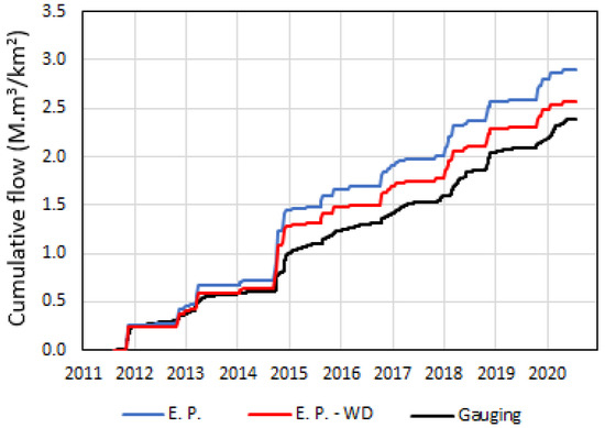
Figure 2.
Example of cumulative curve graph (case of the Salaison River). Gauging = flow rate measured at the gauging station; E. P. = effective precipitation; E. P.-WD = net flow rate potentially induced by precipitation, evapotranspiration, and the water abstractions of surficial and ground water by pumping and diversion.
This kind of graph provides several types of information:
- The reactivity of the watershed to intense rainfall events. Let us remember that the Mediterranean climatic context prevailing in the studied region is characterized by very important and violent rainy events. In such a climate, a “staircase” curve indicates a very reactive watershed where runoff dominates. Conversely, a smooth curve is characteristic of a regularly watered watershed (little impacted by Mediterranean rainfall events) or of a watershed dominated by groundwater flow (base flow in hydrological terminology).
- The relative importance of water abstractions by pumping and diversion in comparison to the effective precipitation volumes. This importance is assessed using the respective heights of the red and blue curves. If these two curves are close, or even merged, it means that the water abstractions are low with regard to the available water. If the distance between the two curves is large, this means that the water abstractions are significant. In such situations, natural water uses may be compromised (sustainability of rivers, support of low-water flows, recharge of wetlands, feeding of riparian vegetation, recharge of aquifers, etc.).
- Representativeness/reliability of the gauging station. If the red and black curves are close, it means that the hydrological functioning of the watershed is in accordance with its extension and rainfall, and that the gauging station measures the entirety of the flows generated by net inputs (rainfall–evapotranspiration–water abstraction).
- The relative importance of external exchanges to the benefit or detriment of the watershed. If the red and black curves are distant, it means that an unknown component of flow exists, i.e., that all flow components are not included within the boundaries. Upstream or lateral inputs may be contributed by neighboring aquifers. Similarly, part of the downstream flows may be subsurface and thus not quantified at the gauging station.
For example, the cumulative curves shown in Figure 2 provide the following interpretation. The effective precipitation curve (in blue) shows the marked effect of Mediterranean rainfall events. This translates into a staircase curve, with each step corresponding to a Mediterranean event. Such events occur mainly in autumn, but sometimes also later in the winter. The Mediterranean episode in the fall of 2014 (640 mm in one month and 270 mm one month later) induced a runoff of more than double that for a normal full year. In this watershed, water abstractions represent one-tenth of the effective precipitation.
The flows recorded at the gauging station (black curve) are 7% lower than the calculated potential flow (net input). This difference may be due to water abstractions being underestimated or to aquifer flow not being measured by the gauging station. Resurgences of water are indeed observed downstream of the station and feed the pond constituting the outlet of the system in a diffuse way. The cumulative flow curve shows the same stair-step shape as the curves calculated from rainfall. This indicates that the flows are rather fast and little dampened by a slow flow through the aquifer. For example, the authors of [36], studying a rainfall-dependent flood regime, noted that a more dampened flow may be due to frequent rainfall or the dominance of ground water contributions.
During 2014 and 2016 autumns, the steps are less pronounced in a measured flow curve than in rainfall-derived curves. This illustrates the local, orographic character of Mediterranean rainfall, where hundreds of mm of rain can fall on one village with almost nothing falling on the neighboring village. In the present case, the weather station probably recorded a very localized thunderstorm that did not occur with this magnitude over the rest of the watershed. Thus, despite the simplicity of these curves and the information they use, the graph can provide a quick decoding of watershed functioning.
A second type of graph (e.g., Figure 3) was built to directly compare the measured cumulative flows (y-axis) to the net input calculated from the rainfall, evapotranspiration, and water abstractions (x-axis). This type of graph is similar to the graphs of the double-mass curves method mentioned in the introduction. We will therefore use this name for this type of graph even if the content is not exactly the same. The proposed graph provides relevant synthetic information without a direct notion of time. It is, however, possible to discuss the interannual variability of the relation between the cumulative data and the effect of a particular hydrological year.
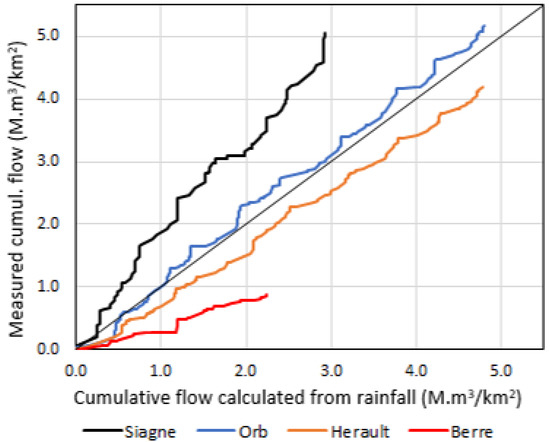
Figure 3.
Example of the double-mass curves of some watersheds.
When the comparative curve is above the 1:1 slope, the measured flows are greater than the potentially expected flows due to rainfall (and vice versa). For example, we can observe in Figure 3 an external water input for the Siagne watershed (and a little for Orb) and, conversely, an external export for the Hérault and Berre watersheds.
This method, in its broad outlines, is close to the one of the double-mass curves [37,38] widely used in hydrological studies (see, for example, [39]). The DMC method uses a cumulative curve of runoff against rainfall. Our method could thus be considered as an extension of this one, but it also incorporates evapotranspiration and water abstractions and represents the two curves in the same unit. Curves can thus be directly compared in terms of flow volumes.
2.3. Studied Watersheds
This method was applied to the main rivers and lagoon tributaries of the French mainland coast of the Mediterranean Sea (Figure 4 and Table 1). The Rhône and Aude rivers were not included in this study because of their significant size and very different hydrological and climatic functioning. The hydrological behavior of these two rivers is, in fact, controlled by the presence of snow on the relief of the Alps and Pyrenees, and by the important modifications of flow induced by the numerous canals used for river navigation, hydroelectric production, and water abstractions for urban, industrial, and agricultural needs. In total, 20 watersheds were studied, of which 11 watersheds were located west of the Rhône River (Occitanie Region) and 9 were located east (Provence, Côte d’Azur Region).
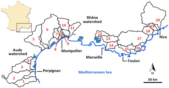
Figure 4.
Location of the studied watersheds along the French Mediterranean coast (watershed numbers refer to Table 1 and were used in the next figures and tables).

Table 1.
Names and areas (at the gauging station) of the studied watersheds.
These watersheds were selected because they have a hydrometric gauging station (Figure 5). Their surface areas vary from 50.8 km2 to 2820 km2. This allowed this method to be tested over a wide range of watershed sizes. The total area investigated was 17,074 km2. In total, 41 weather stations were selected for the calculations (Figure 5). They covered the watersheds with an average density of one station per 420 km2 (one station every 20 km). Due to the different availability of the required data (weather, water abstractions, flow rates), the comparison period was set from August 2011 to July 2020—that is, nine hydrological years (August to July).
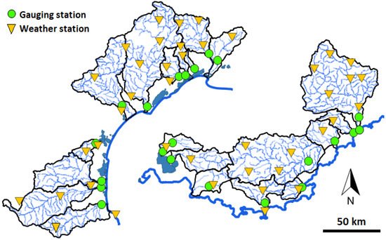
Figure 5.
Location of the gauging and weather stations.
The geological contexts were very diversified and differed according to the watersheds (Figure 6). Most of the terrains had aquifer capacities: quaternary and current alluvium (in light blue on the map); there were also terrains with carbonate dominance (in yellow) or sandstone dominance (in green). Others were rather impermeable: crystalline rocks (in red), volcanic ones (in dark blue), and clayey-schistose terrains (in pink).
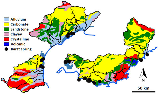
Figure 6.
Geological substratum of watersheds (modified from BRGM map) with the location of the main littoral karst springs.
The geology around the Mediterranean Sea is characterized by the presence of numerous carbonate formations. At the end of the Miocene, during the Messinian period, the Mediterranean dried up because of the reduced inflow of water from the Atlantic through the Betic and Rif straits [40,41]. This allowed the very deep digging of the Mediterranean rivers [42] and the development of karstic networks at depths lower than the current sea level [43,44]. This Messinian karstification was also able to follow, develop, and deepen previous networks set up since the Cretaceous. During the Pliocene, the Mediterranean regained water and submerged overdeepened canyons. This led to the deposition of clayey formations in these rias (submerged valleys) and, often, the clogging of the karst outlets. However, some paleo-valleys and karst networks kept their hydraulic capacity. These structures then allowed the emergence of water into the sea or coastal lagoons [45,46].
On the other hand, the Mediterranean climate is characterized by very dry summers and usually very rainy autumns [46]. Autumn events occur when the continental air mass becomes cold while the Mediterranean is still warm. Such events can bring several hundred mm of rain in a few hours and exceptional floods [47]. During these events, the spatial distribution of the rainfall is very heterogeneous. Rain can be very localized, without spatial continuity [48].
The watersheds, therefore, have more or less important underground components of flow (groundwater) depending on the type of geology involved. The map also shows the main known littoral karst sources. These karst springs are clearly located downstream of large carbonate areas.
3. Results
3.1. Cumulative Curves
Figure 7 shows the cumulative curves calculated for the Var and Loup watersheds. The cumulative curves of the measured (from gauging stations) or calculated (from rainfall) flows show different reactivities (stair step shape). The reactivity is more pronounced for the rainfall-derived curves than from measurements (respectively, red and black curves). Water abstractions are proportionally important in the Loup watershed alone (about a quarter of the calculated available water).
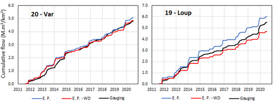
Figure 7.
Cumulative curves of the Var and Loup watersheds.
The comparison of the cumulative curves obtained for the Var River (Figure 7) shows that the water abstraction in this watershed is very low compared to the volume of effective rainfall. Furthermore, the cumulative curve of the flows measured at the outlet is very close to that calculated from rainfall, evapotranspiration, and water abstractions. The reactivity of the curves is also very similar. The hydrological functioning of the watershed thus seems to be well represented by these three components of the water balance.
The water abstractions in the Siagne watershed (Figure 8) represent a small part of the water balance (17%). This river has a cumulative flow measured at the gauging station to be 73% higher than the calculated one. The measured curve is also higher than the cumulative effective precipitation. This can be explained by the fact that this river receives contributions from numerous karst springs: Siagne, Garbo, Pare, Mons, Foux-St-Cézaire, Veyans, etc. According to previous studies [49], the average cumulative flow of these six springs is at least 3.7 m3/s, i.e., a cumulative quantity close to 2.0 M·m3/km2 for nine years. This value is close to the difference observed between the cumulative curves of the Siagne.
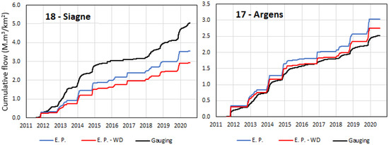
Figure 8.
Cumulative curves of the Siagne and Argens watersheds.
For the Argens watershed (Figure 8), the water abstractions represent a very small part of the water balance (less than 7%). The cumulative curve of the measured flows is slightly lower than that calculated from rainfall, evapotranspiration, and water abstractions. This difference (of about 5%) is within the uncertain range of the knowledge and therefore does not allow for a more detailed analysis of its origin. The cumulative curve of the measured flows is slightly smoother, which seems to indicate a more significant contribution of slow, groundwater flow. Indeed, as noted by [36], a more dampened flow can occur due to frequent rainfall or the dominance of ground water contributions. In Mediterranean watersheds, only the second case can occur.
A good match between the calculated and measured curves was observed for the Giscles and Gapeau watersheds (Figure 9), indicating that there are no significant unknown flows in these watersheds.
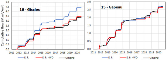
Figure 9.
Cumulative curves of the Giscles and Gapeau watersheds.
For the Huveaune and Arc watersheds (Figure 10), the water abstractions are about 18% of the water balance. The cumulative measured volume of Huveaune is 27% lower than the expected net flow calculated from rainfall. This difference can be explained by the large number of coastal karst springs located south of the watershed (Figure 6). Even if these sources are a little distant from the topographical limits of the watershed, some of them are fed by water from this watershed, as shown by previous colorimetric tracings (in particular, for the submarine spring of Port-Miou [50]). However, no formal quantification of the losses from the Huveaune watershed has been carried out to date. The flow of the Port Miou spring is important (about 7 m3/s) and cannot be attributed to the contribution of the Huveaune watershed alone. Relative to the 154 km2 area of the Huveaune watershed, this flow would indeed represent an equivalent quantity of 8.1 M·m3/km2 for the nine years. This value is considerably higher than the observable difference between the Huveaune curves.
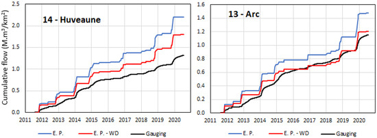
Figure 10.
Cumulative curves of the Huveaune and Arc watersheds.
For the Arc watershed (Figure 10), the measured and calculated cumulative curves are close, but the measured one is more dampened. This would suggest that a significant portion of the flow is underground.
The graph of Touloubre-1 (Figure 11) shows the cumulative curves obtained from the measured and calculated flows for the entire watershed. Water abstractions account for 31% of the effective rainfall. The curve derived from the measurements is very smooth and does not show reactivity to rainfall. The cumulative measured flows are double the volumes calculated from the net rainfall. The difference between the measured and calculated curves is 44 M·m3/year. This reflects the very important input of water due to the irrigation taking place in the Salon-de-Provence sector. The irrigation water comes from the Durance River, which is more than 100 km from the Touloubre watershed. A diagnostic study of the water resource in the Provence region [51] indicated that the volume of irrigation water contributing to the Touloubre watershed is about 86 M·m3/year. According to the same study, the theoretical irrigation needs would be 20 M·m3/year, giving a potential surplus of irrigation of 66 M·m3/year. This surplus can explain the difference observed between the curves.
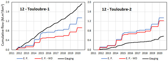
Figure 11.
Cumulative curves of the Touloubre watershed.
Another gauging station (Touloubre-2) exists 12 km northeast of the first station, 22 km upstream along the Touloubre River and upstream from the irrigation zone of Salon-de-Provence. At this gauging station (plot Touloubre-2 on Figure 11), the respective heights of the cumulative curves are reversed between measured and calculated flows. The difference between both curves is 18 M·m3/year. This deficit of 18 M·m3/year and the surplus of 44 M·m3/year observed at the downstream station globally balance the irrigation surplus of 66 M·m3/year provided between the two stations. Karst springs are known to exist downstream of the station Touloubre-2 [52]. Flows of about 500 l/s have been reported for the Calissane spring and flows of at least 50 l/s have been reported for the underwater springs of St-Chamas. These flows (>17 M·m3/year) are of the same order of magnitude as the deficit noted (18 M·m3/year).
For the Vistre watershed (Figure 12), the cumulative measured flow is 29% higher than the calculated water volume and very dampened. This seems to show that a significant portion of water could come from outside the watershed and that groundwater plays an important role. This watershed mainly lies on quaternary alluvium (shown in blue in Figure 6). North-west of this watershed, there is karstified limestone (shown in yellow in Figure 6). Karstic manifestations exist (such as the Fountain of Nimes), but none of them provide a significant localized flow. The contribution of limestone to the watershed has been stated by some works (e.g., [53,54]) but never quantified.
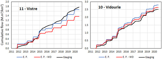
Figure 12.
Cumulative curves of the Vistre and Vidourle watersheds.
The three cumulative curves of the Vidourle watersheds (Figure 12) are close, indicating that the water abstractions are small and that there are no significant unknown flows. The measured cumulative curve is almost as responsive to rainfall events as the calculated curve.
The water abstractions in the Salaison watershed (Figure 13) are small, and the measured cumulative curve is close to the calculated one. The difference is mainly due to the fact that the gauging station is not located at the outlet of the watershed and that groundwater flows directly downstream.
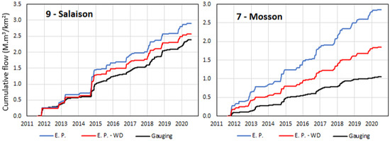
Figure 13.
Cumulative curves of the Salaison and Mosson watersheds.
The Mosson watershed (Figure 13) shows significant water abstractions and a measured curve much lower than expected (43% lower). This lack of measured water is due to karstic losses taking place in this watershed. These losses feed karst springs existing in the immediate southwest of the watershed (Figure 6). This relation has been demonstrated by tracing. The average flow rates of the downstream karst springs (Vène, Issanka, Vise, etc.) are not precisely known but would be in the order of few m3/s [55,56]. Part of this flow is taken for drinking water, while the rest feeds the pond of Thau located downstream.
For the Lez watershed (Figure 14), the most downstream gauging station (Lez-1 on Figure 9) provides a measured cumulative curve that does not have the same shape as the calculated one. On the other hand, the station located just a little further upstream (Lez-2) gives a measured curve that is more consistent in shape with the calculated one, though still above it. The Lez flow is disturbed by three different sources of water: (1) the contribution of the Lez karstic source (and other small, diffuse karstic emergences), (2) an artificial contribution of water (from the irrigation canal) intended to support the low flow of the river, and (3) an exacerbation of runoff related to the sealing of urban areas. The first contribution explains the shape of the Lez-2 curve.
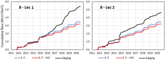
Figure 14.
Cumulative curves of the Lez watershed.
The natural average flow of the Lez spring would be 1.8 m3/s, i.e., nearly 60 M·m3/year [57]. Of this annual volume, 33 M·m3/year is withdrawn by the Montpellier Metropolitan Area and subtracted from the watershed. The remaining flow contributed to the watershed is therefore 27 M·m3/year, i.e., 1.4 M·m3/km2 for nine years, which is approximately the observed difference between the measured and calculated cumulative curves of Lez-2.
The particular shape of the Lez-1 curve cannot be explained by the two first contributions mentioned above (the karst spring and the water intake from the canal). The first contribution (karst spring) should give a curve shape equivalent to the Lez-2 curve. The water supplied for low-water support would occur during the summer and not during the winter and fall, as observed from the curve. The only possible explanations could be the occurrence of rainfall only on the downstream side of the watershed (which was not observed by the meteorological stations used) and/or the exacerbation of runoff related to the sealing of urban areas. A problem with the gauging station also cannot be excluded.
The Orb curves (Figure 15) fit very well, indicating that there is a priori no gain or loss of water in this watershed. The Hérault river shows a cumulative curve measured at the outlet of the watershed (Gauging_1 on the plot) that is lower than the one expected (1.1 M·m3/km2 over the nine years). However, the gauging station located slightly upstream shows a smaller difference (0.5 M·m3/km2). The downstream part of the watershed is, in fact, made up of alluvial deposits, allowing the river to feed the water table. Some of the water coming from the watershed flows through the groundwater and is not measured at the gauging station.
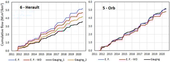
Figure 15.
Cumulative curves of the Hérault and Orb watersheds.
Furthermore, the waters of the Lez karstic source mentioned above come from the upstream Hérault watershed. The natural average flow of this spring would be 1.8 m3/s, i.e., nearly 60 M·m3/year. The 60 M·m3/year found represents, for gauging station Gauging_2, a cumulative quantity of 0.23 M·m3/km2 over the nine years, i.e., half the difference between the measured and calculated curves. The flow deficit at the most downstream station (Gauging_1) would thus correspond to the contribution to the Lez spring system [57] and to the underground flow in the coastal plain [58].
The Berre river (Figure 16) has a very low cumulative measured flow (about 61% lower than the calculated one). This is due to the presence of a great deal of karstic loss taking place in this watershed. These losses are mainly located in the downstream part of the watershed. Their existence is confirmed by observations, but their importance has never been formally quantified, except through the flows measured at the two existing gauging stations. Numerous littoral karst springs with significant flow rates exist east of the Berre watershed (Figure 6). Unfortunately, no confirmation nor quantification of the direct contribution of this watershed have been provided to date (e.g., by carrying out colorimetric tracings). The known flows of the nearby springs are significant: about 0.6 m3/s for the karst springs near La Palme lagoon [59] and about 2 m3/s and 1 m3/s for the Font-Estramar and Font-Dame springs feeding the Salses-Leucate lagoon, respectively.
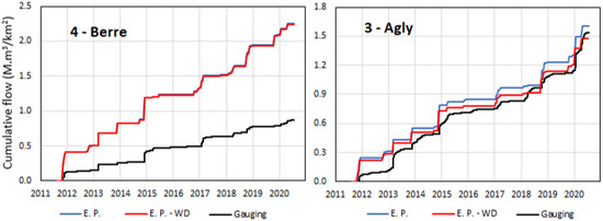
Figure 16.
Cumulative curves of the Berre and Agly watersheds.
For Agly river (Figure 16), the measured and calculated curves fit relatively well.
The cumulative flow curves measured for the Tech and Têt rivers (Figure 17) are slightly higher compared to those estimated from the rainfall, while the one for the Berre river is significantly lower. For Agly river, both curves are very close. For the Tech and Têt rivers, the difference between the curves is due to the lack of weather stations on the Pyrenean reliefs, where precipitation is more abundant. This leads to a slight underestimation of the calculated flows, since the areas with a high rainfall are not correctly taken into account.
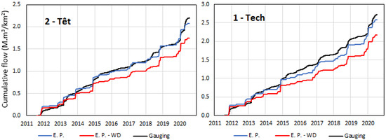
Figure 17.
Cumulative curves of the Têt and Tech watersheds.
Figure 18, left, shows that the cumulative measured flows of these watersheds have a decreasing trend from south (i.e., from Tech) to north (i.e., to Berre). This trend is not observed for rainfall estimated flows (Figure 18, right). The most watered watersheds are the Tech and Berre ones. The Tech watershed receives more significant precipitation because of the barrier effect induced by the Pyrenees chain. On the other hand, the Berre is much more subject to Mediterranean rainfall episodes than the others because of the wind direction during these periods (towards the north). The regular decrease in cumulative flow observed from south to north results from the combination of the regional rainfall distribution and the relative proportion of permeable rocks in the different watersheds (% of alluvium or carbonate; see Figure 6). The southern watersheds are mainly composed of crystalline rocks and shales, while the northern watersheds are mainly made up of alluvium and carbonates.
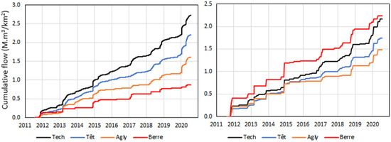
Figure 18.
Cumulative curves of measured flows (left) and calculated ones from rainfall (right) for west watersheds (near Perpignan).
3.2. Double-Mass Curves
Figure 19 shows the double-mass curves obtained for the east watersheds (between Toulon and Nice). These curves show the good global fit between the measured and calculated flows, except for the Siagne river. In this watershed, the measured fluxes are higher than those estimated from rainfall, as discussed above. For all other watersheds, the observations are consistent with the estimates. In the latter case, this does not mean that there is no unknown input or output, but that these compensate for each other if they exist. The curves are not very linear (smooth), showing oscillations or steps. These variations indicate that the two cumulative curves are not identical. In this case, the calculated cumulative curves showed steps related to Mediterranean rainfall events, unlike the measured cumulative curves, which were smoother. This can still partly be seen in the double-mass curves.
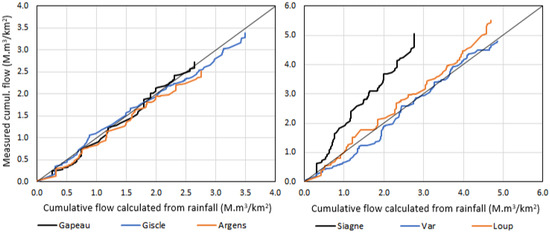
Figure 19.
Double-mass curves of the east watersheds (between Toulon and Nice).
The double-mass curves of watersheds located near Marseille (Figure 20) confirm the good fit of the cumulative data for the Arc watershed and the reduced measured flow for the Huveaune river, while the Touloubre one shows an increased or diminished flow according to the gauging station used. The staircase steps are very marked in the case of Touloubre 1, indicating the lack of similarity between the measured and calculated cumulative flows. For Touloubre 2, the steps are less marked, indicating the better similarity of the measured and calculated flows.
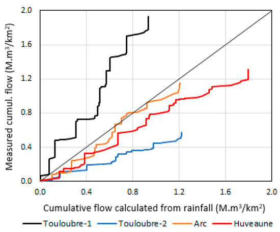
Figure 20.
Double-mass curves of the near-east watersheds (near Marseille).
The Double-mass curves of the watersheds located around Montpellier (Figure 21) confirm the previous findings: a good adjustment for Orb, Vidourle, and Salaison; increased measured flows for Lez and Vistre; and reduced measured flows for Hérault and Mosson. Some curves are relatively linear (smoothed), indicating a flow that is fairly well correlated to rainfall events. Others show a more oscillating curve, indicating measured flows that are more buffered from rain events.
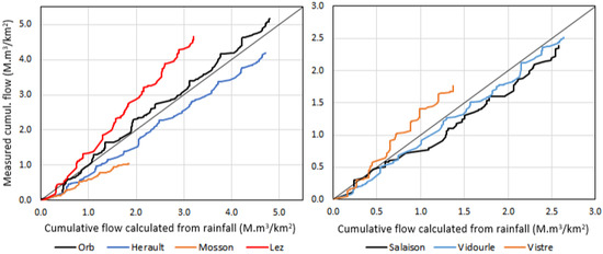
Figure 21.
Double-mass curves of near-west watersheds (west of Montpellier).
The double-mass curves (Figure 22) of these western watersheds confirm the fairly good adjustment made for the Tech, Têt, and Agly rivers and the very reduced flow measured for the Berre. The Tech and Têt curves are relatively linear (smoothed), reflecting a less Mediterranean rainfall pattern, whereas the curves of the other two watersheds present more marked steps typical of the Mediterranean regime.
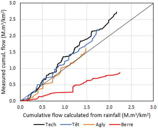
Figure 22.
Double-mass curves of west watersheds (near Perpignan).
3.3. Comparison of Decadal Increases in Cumulative Curves
The flow data were used to calculate explanatory coefficients of the hydrological functioning of the watershed. Four steps were taken: (1) the extraction of decadal increases in each measured or calculated cumulative curve (i.e., 324 values for each 9-year curve); (2) the determination of the mean value and standard deviation of each data series; (3) the calculation of the coefficient of variation as the ratio between the standard deviation and the mean value; (4) the calculation of the ratio between the mean values of measured and calculated data (and the same for the coefficient of variation). The coefficient of variation makes it possible to assess the dispersion of values around the mean in a dimensionless way (whatever the value of the average or the unit of measurement used). This makes it possible to compare data series and the watersheds between them. Table 2 shows the statistics and ratios obtained.
Table 2.
Statistics of decadal increases in measured and calculated flows (STD = standard deviation; CV = coefficient of variation = STD/mean value).
The calculated ratios were ranked in ascending order. Figure 23 shows the ranked ratios calculated with the mean values of measured and calculated decadal increases. Each mean value represents the average growth rate of the cumulative curve. The ratio between the two mean values thus illustrates the relative growth of the two curves. It indicates whether one curve is growing faster than the other, and, if so, which one. For example, the mean increase in the measured cumulative curve of the Berre River is 0.4 times that of the calculated curve. This means that the measured flow curve grows 60% slower than the calculated flow curve. The outfall is therefore missing 60% of the water that is likely to reach it. In contrast, the mean increase in the measured cumulative curve of the Siagne River is 1.7 higher than the calculated one. This means that the measured flow curve grows 70% faster than the calculated flow curve. The outlet therefore has 70% more water than it should receive due to the water balance.
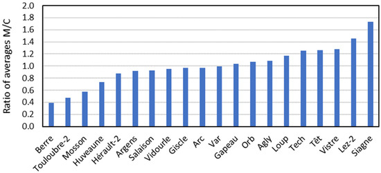
Figure 23.
Ratios of the mean decadal increases in measured and calculated cumulative flows.
The watersheds with the lowest average value ratios (left in the graph) are those for which a significant unknown output exists. This may correspond to losses from the watershed feeding a karst spring located downstream, outside the watershed. Conversely, the highest ratios are those with unknown inputs or visible inputs but that are not related to the rain falling on the watershed (e.g., upstream karst spring fed by a neighboring watershed). Watersheds with a ratio of between 0.9 and 1.1 (or between 0.8 and 0.12 depending on the accepted precision) are considered not to have significant unknown exchanges with the outside. More than half of the watersheds fall within this range. Four watersheds have a clear deficit in their measured balance (left in the graph), while five watersheds have a surplus (right in the graph), two of which have a large surplus.
On the other hand, the coefficient of variation CV (i.e., the ratio of the standard deviation to the mean value) was calculated for the decadal increases in each cumulative curve of the measured or calculated flows. These CVs represent the dispersion of the decadal increase values on a curve. The smoother the curve is, the lower the CV value is. A low CV (i.e., a smooth curve) indicates that the flows are very dampened, i.e., dominated by a low flow, such as through a groundwater component. Conversely, a high CV indicates a sawtooth curve dominated by the influence of rainfall, i.e., by rapid flow. The ratios of the CVs obtained for the two curves of measured vs. calculated flows were calculated and ranked. Figure 24 shows the ranked ratios obtained for the 20 watersheds.
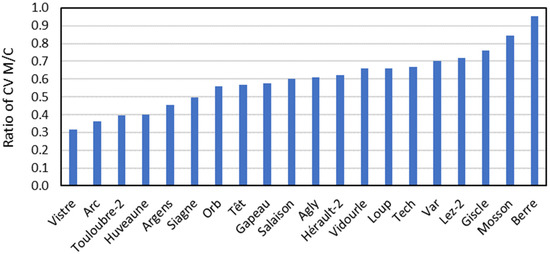
Figure 24.
Ratios of the coefficients of variation for the decadal increases in measured and calculated cumulative flows.
This ratio allows us to assess the relative importance of the slow and fast components of flow in the watersheds. Indeed, a ratio close to 1 indicates that the curve of the measured flows is as irregular (sawtooth shape) as the derived rainfall curve. The flows at the outlet are therefore directly influenced by the rainfall events falling on the watershed. In this case, the functioning of the watershed is dominated by rapid flows. These can be related to rapid surface runoff or karst flows. The Berre watershed has a ratio close to 1, indicating that the flow observed at the gauging station has a reactivity close to the temporal distribution of rainfall.
Conversely, a very low ratio indicates that the measured flow curve is much smoother than that derived from rainfall. In this case, the proportion of slow flow is important. This generally indicates that the groundwater component in porous, non-karstic aquifers is important. This may also be due to flows being slowed by thick soils or dense vegetation, which is not the case in the Mediterranean watersheds studied. The Vistre and Arc watersheds present very smooth cumulative curves, i.e., flows strongly dampened against rainfall. The slow subsurface component of these watersheds thus, appears to dominate their functioning.
The ratio of the CVs of the decadal increases in measured and calculated cumulative curves seems to be correlated with the respective part of fast and slow flows. It could be used to provide a more quantitative estimation of the repartition of the flows between fast and slow components. However, this would require further investigations and a comparison with more accurate quantification conducted using other approaches, such as hydrological modeling.
Figure 25 compares the ratios of the mean values and CV calculated from the decadal increases in the measured and calculated cumulative flows. This plot summarizes all the information resulting from the method, namely (along the x-axis), the representativeness of the flows measured by the gauging station (compared to the calculated flows), and (along the y-axis) the fraction of fast flows taking place in the watershed. The watersheds on the left of the plot are those with measured runoff deficits (unknown outputs), with those on the right having excess runoff (unknown inputs). The watersheds at the top of the graph are those dominated by slow flows (smooth cumulative curves), while those at the bottom are dominated by fast flows (stair step curves).
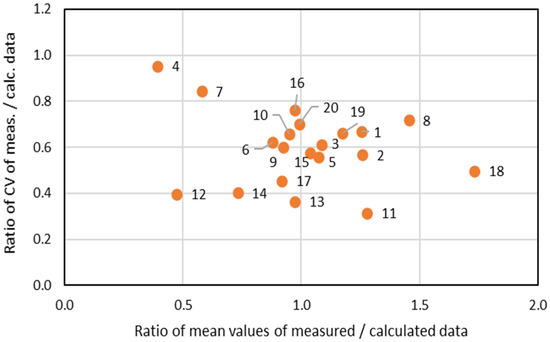
Figure 25.
Comparison of the ratios of the mean values and those of the coefficients of variation calculated from the decadal increases in measured and calculated cumulative flows (numbers are those of the watershed).
4. Discussion
The application of the proposed method in 20 watersheds with different sizes, geology, and climatology showed that it could quickly identify the existence of hidden external components of flow and evaluate their magnitude. The comparison of the curves also allows us to estimate the relative importance of groundwater in the flows, since this component of flow will be slower and contribute to more dampened curves. The smoothest curves do not necessarily correspond to the largest watersheds, for which one might think that the flows would be more dampened. On the other hand, the less smooth curves (sawtooth shape) do not correspond to the smallest watersheds for which one could expect the runoff to be very fast; thus, they follow the same evolution as the rain.
For the studied Mediterranean watersheds, water inflows from outside the topographic watershed mainly occur due to upstream karst springs (which are fed by water from outside the topographic watershed) or because of irrigation water imported from another distant watershed. Water outflows outside the topographic watershed occur due to karstic circulations or deep underground flows. In one case, a transfer takes place between two adjacent watersheds (Hérault and Lez).
The results presented above compared the 9-year cumulative curves calculated from the flows measured at the watershed outlets and from rainfall, evapotranspiration, and water abstractions. These curves are expressed in M·m3/year per km2 of the watershed in order to allow comparisons to be made between the watersheds. The difference between the two cumulative volumes was calculated and expressed in M·m3/year, taking into account the watershed area. This difference corresponds to the annual volumes of water that cannot be explained by the rain falling on the topographic watershed, the evapotranspiration, and the water abstractions. This difference represents flows whose origin or fate is generally unknown.
Table 3 summarizes the cumulative volumes measured at the gauging stations located at the outlet of the watersheds and those calculated from rainfall, evapotranspiration, and water abstraction. The differences between both volumes are also indicated.
Table 3.
Quantitative summary of the comparison between measured and calculated flows.
Table 4 compares the annual volume of unknown flows (out of the known components of water balance) estimated by the method with the karst spring flows and other volumes of water exchanged, as reported by previous studies. The volumes reported by previous studies are data that have been measured (especially in the case of surface karst springs or irrigation inputs) or only estimated (in the case of submarine springs or diffuse inputs or outputs). The references for this knowledge are given in the last column of Table 4. Most of these are reports from public institutions and can be downloaded from the internet.
Table 4.
Comparison of the estimated unknown components of the water balance to the flows reported in the literature.
These estimated and reported annual flows are plotted in Figure 26. The orders of magnitude between both flows are similar, despite the simplicity of the proposed approach and the fact that many of the reported flows are estimates. This favorable comparison shows that the proposed method could be used as a first approach to identify and estimate the importance of possible unknown flows taking place in a topographic watershed.
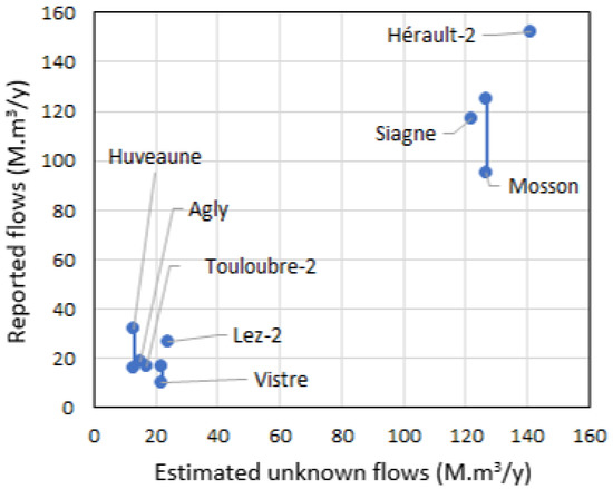
Figure 26.
Comparison between the unknown component of the water balance estimated with the method and the flows reported in the literature (flows in M·m3/y).
The same results are expressed in M·m3/y/km2 to allow comparison between watersheds and plotted in Figure 27. In this graph, the points are distributed differently from the previous figure but again show a favorable comparison between the estimated and reported quantities. The linear regression performed on these points gives a good correlation coefficient (R2 = 93%).
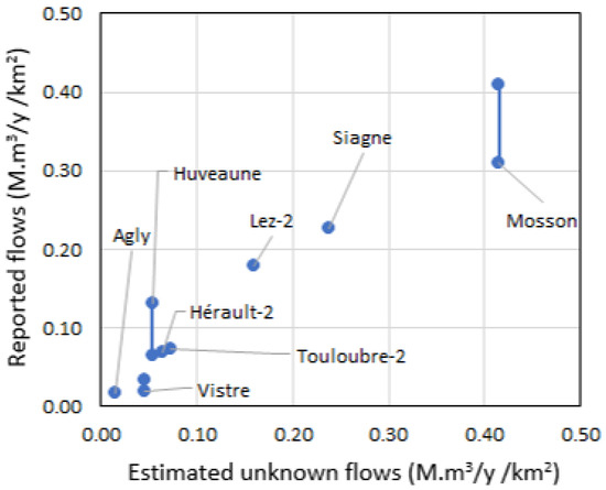
Figure 27.
Comparison between the unknown component of the water balance estimated with our method and the flows reported in the literature (expressed in M·m3/y/km2).
5. Conclusions
In this paper, we proposed a rapid method for diagnosing the hydrological balance of topographic watersheds. This method is based on the use of knowledge that is generally available at the watershed scale: rainfall, potential evapotranspiration, water abstraction, and flow at the outlet. In order to remove the transient components of the water fate (such as interception, depression storage, soil storage variation, and groundwater storage variation), this method uses cumulative curves of water volumes over periods of several years. On this time scale, the variations occurring due to these components are compensated for over time or their effect becomes negligible.
This method requires data that are easily accessible thanks to numerous internet databases. Rainfall and evapotranspiration data are the most easily and widely available information. They can be obtained from the weather stations of national, regional, or local services, or even now from many private stations, such as those of farmers. In cases where no weather station exists, it is possible to use weather radar data. Knowledge of water abstractions requires that they be reported, at least for the largest ones. For some purposes, such as irrigation, an estimate of abstractions can be made with an acceptable range of error. For small abstractions scattered over a watershed, a statistical approach can be implemented to assess its overall importance.
Knowledge of river flow rates requires the existence of a gauging station, which cannot be replaced by another source of information. On the other hand, this suggests the possibility of using an adaptation of this method to estimate the magnitude of flow in ungauged watersheds. In such watersheds, knowledge of the existence and importance of external inputs or exports could make it possible to quickly obtain a fairly reliable estimate of the water flows involved. This could be the case, for example, when characterizing the importance of nutrient fluxes contributed by an ungauged river. Combining net water inputs with nutrient concentrations measured in the river would provide a relevant estimate of potential fluxes.
If all components of the water balance are well known, the cumulative volumes calculated from rainfall, evapotranspiration, and water abstraction data should be similar to the cumulative volumes of measured flows. When the cumulative volumes significantly differ, one may suspect that unknown inflows or outflows of water exist. Such exchanges with areas outside of the topographic watershed may exist, especially when karst flows occur. This is frequently the case in Mediterranean basins due to the Messinian crisis, which led to the drying of the Mediterranean and the creation of important deep karst networks. The exchanges occurring between topographic watersheds, however, do not only occur due to karst flows but can also be related to inter-basin water transfer for irrigation purposes or to deep groundwater flows.
The application of the proposed method on 20 Mediterranean topographic watersheds has shown that it can help to identify the existence of unknown components of the water balance at the topographic watershed scale. In this type of watershed, the possibility of karst flows is known but they are often difficult to identify and estimate because they cannot always be located and are not always visible. Except in the case where water inflows induce important karstic springs, the contributions from neighboring watersheds can be very diffuse and are often localized in the riverbed itself. In this case, only serial gaugings can make it possible to locate and quantify them. On the other hand, the water losses are also often diffuse along the stream and can only be quantified by extensive field investigations. The favorable comparison obtained between the unknown component of the water balances estimated by the proposed method and the reported flows seems to show that this method can help to estimate the order of magnitude of the unknown component of flows involved in the water balance of a topographic watershed.
The cumulative curves obtained allow us to assess the relative importance of slow and fast flows taking place in watersheds. This can be assessed with the coefficient of variation (CV = ratio of the standard deviation to the mean) of the decadal increases in the two cumulative curves of the measured and calculated flows. If the CV obtained from measurements is close to that derived from rainfall, this indicates that the flows are rapid (dominated by runoff) and that the proportion of groundwater flow is rather low. If the CVs are very different, this is because the measured flow curve is more dampened than the one derived from rainfall, and the underground flows are important. This situation prevails in watersheds where the flows have not been modified (or only slightly) by hydraulic developments. If these developments have significantly changed the flow dynamics, the CVs cannot be compared.
Stream gauging data may have uncertainties related to the hydrometric station, the establishment of rating curves, the measuring instruments used, etc. The same is true for the estimation of flows by mathematical simulation models. The proposed method cannot avoid the existence of uncertainties and possible biases, but constitutes a simple and operational tool that completes the panel of methods available for the characterization of the water balance of watersheds. It represents a first approach for the quantification of flows and help guide the implementation of more sophisticated approaches. The proposed method does not allow a formal quantification of the different components of flows, only the identification of their possible existence and their relative order of magnitude. It allows us, for example, to say whether fast or slow flows dominate the functioning of a watershed. As with all methods, sufficient and reliable data must be available for this approach to be used. However, the required data are generally available for most watersheds, at least for those with a size of several tens to hundreds of km2.
The proposed method is a simple approach that can be used to characterize the hydrological functioning of a watershed. It can help actors to understand the global behavior of a system and to identify the specificities and particularities of this functioning that will influence and condition the reflections and actions that will follow. For example, one can think of studies aimed at establishing concerted management plans for water resources imposed by the European Water Framework Directive 2000/60/EC of 23 October 2000. In France, these European directives have been translated into the Basic Guidelines of the Master Plans for Water Development and Management (SDAGE-OF). This method has been applied with success in Mediterranean watersheds. However, it should be tested on other non-karstic and non-Mediterranean watersheds in order to study its applicability and relevance in other contexts. It should also be applied to watersheds where detailed hydrological modeling has been carried out before. This will allow us to verify, and possibly calibrate, the estimates of the respective contributions of fast and slow flows by comparison with the results obtained by modeling.
Author Contributions
Conceptualization, O.B., S.S.-P., A.G. and S.S.; methodology, O.B. and S.S.-P.; validation, A.G. and S.S.; writing—original draft preparation, O.B. and S.S.-P.; writing—review, A.G. and S.S.; project administration, A.G. and S.S. All authors have read and agreed to the published version of the manuscript.
Funding
This study was carried out thanks to the funding of the Rhône Méditerranée Corse Water Agency.
Institutional Review Board Statement
Not applicable.
Informed Consent Statement
Not applicable.
Data Availability Statement
The data used in this paper are available free of charge on the internet for hydrometric flow and water abstraction data, and for a fee for meteorological data. The websites are indicated in the bibliographic references at the end of the paper.
Conflicts of Interest
The authors declare no conflict of interest.
References
- European Commission. Guidance Document on the Application of Water Balances for Supporting the Implementation of the WFD; Technical Report—2015—090, Final—Version 6.1—18/05/2015; European Commission, Directorate-General for Environment, Publications Office: Brussel, Belgium, 2016. [Google Scholar] [CrossRef]
- Kampf, S.K.; Burges, S.J.; Hammond, J.; Bhaskar, A.; Covino, T.P.; Eurich, A.; Harrison, H.; Lefsky, M.; Martin, C.; McGrath, D.; et al. The Case for an Open Water Balance: Re-envisioning Network Design and Data Analysis for a Complex, Uncertain World. Water Resour. Res. 2020, 56, e2019WR026699. [Google Scholar] [CrossRef]
- Bassi, N.; Harish Kumara, B.K.; Sahasranaman, M.; Ganguly, A. Comment: Getting the Methodology Wrong for Analysing the Hydrological Changes in Watersheds. Hydrol. Earth Syst. Sci. Discuss. 2018, 187, 1–11. [Google Scholar] [CrossRef] [Green Version]
- Fan, Y. Are catchments leaky? Wiley Interdiscip. Rev. Water 2019, 6, e1386. [Google Scholar] [CrossRef]
- Le Mesnil, M.; Moussa, R.; Charlier, J.-B.; Caballero, Y. Impact of karst areas on runoff generation, lateral flow and interbasin groundwater flow at the storm-event timescale. Hydrol. Earth Syst. Sci. 2021, 25, 1259–1282. [Google Scholar] [CrossRef]
- Fan, Y.; Toran, L.; Schlische, R.W. Groundwater flow and groundwater-stream interaction in fractured and dipping sedimentary rocks: Insights from numerical models. Water Resour. Res. 2007, 43. [Google Scholar] [CrossRef]
- Rivera, A. Transboundary aquifers along the Canada–USA border: Science, policy and social issues. J. Hydrol. Reg. Stud. 2015, 4, 623–643. [Google Scholar] [CrossRef] [Green Version]
- Neilson, B.T.; Tennant, H.; Stout, T.L.; Miller, M.P.; Gabor, R.S.; Jameel, Y.; Millington, M.; Gelderloos, A.; Bowen, G.J.; Brooks, P.D. Stream Centric Methods for Determining Groundwater Contributions in Karst Mountain Watersheds. Water Resour. Res. 2018, 54, 6708–6724. [Google Scholar] [CrossRef]
- Kačaroğlu, F. Review of Groundwater Pollution and Protection in Karst Areas. Water, Air, Soil Pollut. 1999, 113, 337–356. [Google Scholar] [CrossRef]
- Longenecker, J.; Bechtel, T.; Chen, Z.; Goldscheider, N.; Liesch, T.; Walter, R. Correlating Global Precipitation Measurement satellite data with karst spring hydrographs for rapid catchment delineation. Geophys. Res. Lett. 2017, 44, 4926–4932. [Google Scholar] [CrossRef]
- Hartmann, A.; Goldscheider, N.; Wagener, T.; Lange, J.; Weiler, M. Karst water resources in a changing world: Review of hydrological modeling approaches. Rev. Geophys. 2014, 52, 218–242. [Google Scholar] [CrossRef]
- Dhungel, R.; Fiedler, F. Water balance to recharge calculation: Implications for watershed management using systems dynamics approach. Hydrology 2016, 3, 13. [Google Scholar] [CrossRef] [Green Version]
- Gonzales, A.L.; Nonner, J.; Heijkers, J.; Uhlenbrook, S. Comparison of different base flow separation methods in a lowland catchment. Hydrol. Earth Syst. Sci. 2009, 13, 2055–2068. [Google Scholar] [CrossRef] [Green Version]
- Jakada, H.; Chen, Z.; Luo, M.; Zhou, H.; Wang, Z.; Habib, M. Watershed Characterization and Hydrograph Recession Analysis: A Comparative Look at a Karst vs. Non-Karst Watershed and Implications for Groundwater Resources in Gaolan River Basin, Southern China. Water 2019, 11, 743. [Google Scholar] [CrossRef] [Green Version]
- Bayou, W.; Wohnlich, S.; Mohammed, M.; Ayenew, T. Application of Hydrograph Analysis Techniques for Estimating Groundwater Contribution in the Sor and Gebba Streams of the Baro-Akobo River Basin, Southwestern Ethiopia. Water 2021, 13, 2006. [Google Scholar] [CrossRef]
- McCallum, A.M.; Andersen, M.S.; Kelly, B.F.; Giambastiani, B.M.; Acworth, R. Hydrological Investigations of Surface Water-Groundwater Interactions in a Sub-Catchment in the Namoi Valley, NSW, Australia; Presented at Cotton Catchment Communities CRC, 2009 Science Forum, Narrabri, NSW, 17–19 August 2009; IAHS-AISH Publication: Narrabri, Australia, 2009; pp. 157–166. [Google Scholar]
- Andersen, M.S.; Acworth, R.I. Stream-aquifer interactions in the Maules Creek catchment, Namoi Valley, New South Wales, Australia. Appl. Hydrogeol. 2009, 17, 2005–2021. [Google Scholar] [CrossRef]
- Triana, J.S.A.; Chu, M.L.; Guzman, J.A.; Moriasi, D.N.; Steiner, J.L. Beyond model metrics: The perils of calibrating hydrologic models. J. Hydrol. 2019, 578, 124032. [Google Scholar] [CrossRef]
- Wang, Y.; Chen, N. Recent progress in coupled surface–ground water models and their potential in watershed hydro-biogeochemical studies: A review. Watershed Ecol. Environ. 2021, 3, 17–29. [Google Scholar] [CrossRef]
- Gayathri, K.D.; Ganasri, B.P.; Dwarakish, G.S. A Review on Hydrological Models. International Conference on Water Resources, Coastal and Ocean Engineering (ICWRCOE 2015). Aquatic Procedia. 2015, 4, 1001–1007. [Google Scholar] [CrossRef]
- Kannan, N.; Santhi, C.; White, M.J.; Mehan, S.; Arnold, J.G.; Gassman, P.W. Some Challenges in Hydrologic Model Calibration for Large-Scale Studies: A Case Study of SWAT Model Application to Mississippi-Atchafalaya River Basin. Hydrology 2019, 6, 17. [Google Scholar] [CrossRef] [Green Version]
- Bailey, R.T.; Wible, T.C.; Arabi, M.; Records, R.M.; Ditty, J. Assessing regional-scale spatio-temporal patterns of groundwater-surface water interactions using a coupled SWAT-MODFLOW model. Hydrol. Processes 2016, 30, 4420–4433. [Google Scholar] [CrossRef]
- Dudai, Y.; Evers, K. To Simulate or Not to Simulate: What Are the Questions? Neuron 2014, 84, 254–261. [Google Scholar] [CrossRef] [PubMed] [Green Version]
- Ahiablame, L.; Chaubey, I.; Engel, B.; Cherkauer, K.; Merwade, V. Estimation of annual baseflow at ungauged sites in Indiana USA. J. Hydrol. 2013, 476, 13–27. [Google Scholar] [CrossRef]
- Lee, H.; Choi, H.-S.; Chae, M.-S.; Park, Y.-S. A Study to Suggest Monthly Baseflow Estimation Approach for the Long-Term Hydrologic Impact Analysis Models: A Case Study in South Korea. Water 2021, 13, 2043. [Google Scholar] [CrossRef]
- Magyar, N.; Hatvani, I.; Arató, M.; Trásy, B.; Blaschke, A.; Kovács, J. A New Approach in Determining the Decadal Common Trends in the Groundwater Table of the Watershed of Lake “Neusiedlersee”. Water 2021, 13, 290. [Google Scholar] [CrossRef]
- Online Etymology Dictionary. Available online: https://www.etymonline.com/word/watershed (accessed on 4 February 2022).
- Available online: https://a4ws.org/wp-content/uploads/2018/09/AWS_Guidance_Catchments_20180831.pdf (accessed on 4 February 2022).
- Raynaud, F.; Mathieu-Subias, H.; Borrell-Estupina, V.; Pistre, S.; Seidel, J.-L.; Van-Exter, S.; de Montety, V.; Hernandez, F. Influence of Karstic System on Surface Flooding in Mediterranean Climate. In Engineering Geology for Society and Territory—Volume 3; Lollino, G., Arattano, M., Rinaldi, M., Giustolisi, O., Marechal, J.C., Grant, G., Eds.; Springer: Cham, Switzerland, 2014. [Google Scholar] [CrossRef]
- Vakanjac, V.R.; Prohaska, S.; Polomčić, D.; Blagojevic, B.; Vakanjac, B. Karst aquifer average catchment area assessment through monthly water balance equation with limited meteorological data set: Application to Grza spring in Eastern Serbia. Acta Carsologica/Karsoslovni Zb. 2013, 42. [Google Scholar] [CrossRef] [Green Version]
- Geng, X.; Zhang, C.; Zhang, F.; Chen, Z.; Nie, Z.; Liu, M. Hydrological Modeling of Karst Watershed Containing Subterranean River Using a Modified SWAT Model: A Case Study of the Daotian River Basin, Southwest China. Water 2021, 13, 3552. [Google Scholar] [CrossRef]
- French Water Abstraction Data. Available online: https://bnpe.eaufrance.fr (accessed on 15 December 2021).
- French Meteorological Data. Available online: https://publitheque.meteo.fr (accessed on 15 December 2021).
- French Soil Data in Cartographic Format. Available online: https://agroenvgeo.data.inra.fr (accessed on 15 December 2021).
- French Hydrologic Data. Available online: https://hydro.eaufrance.fr (accessed on 15 December 2021).
- Hailegeorgis, T.T.; Alfredsen, K.; Killingtveit, A. Appraisal of a Comprehensive Framework of Decision Support System (DSS) for Hydropower in Africa: The Influential Roles of Hydrology for Optimal and Sustainable Planning-Management and Potential Conflict Resolution among Water Uses/Users and Case Studies for Catchments in Ethiopia and Norway. November 2019. In Proceedings of the DSS for Hydropower in Africa. Project: Hydrology and Hydropower in Africa. Available online: https://www.researchgate.net/publication/336995275 (accessed on 4 February 2022).
- Merriam, C.F. A comprehensive study of the rainfall on the Susquehanna Valley. Trans. Am. Geophys. Union 1937, 18, 471–476. [Google Scholar] [CrossRef]
- Searcy, J.K.; Hardison, C.H.; Langein, W.B. Double-mass curves, with a section fitting curves to cyclic data. Gen. Surf.-Water Tech. 1960, 1541, 31–66. [Google Scholar] [CrossRef]
- Li, R.; Huang, H.; Yu, G.; Yu, H.; Bridhikitti, A.; Su, T. Trends of Runoff Variation and Effects of Main Causal Factors in Mun River, Thailand During 1980–2018. Water 2020, 12, 831. [Google Scholar] [CrossRef] [Green Version]
- Krijgsman, W.; Hilgen, F.J.; Raffi, I.; Sierro, F.; Wilson, D.S. Chronology, causes and progression of the Messinian salinity crisis. Nature 1999, 400, 652–655. [Google Scholar] [CrossRef] [Green Version]
- Rouchy, J.M.; Caruso, A. The Messinian salinity crisis in the Mediterranean basin: A reassessment of the data and an integrated scenario. Sediment. Geol. 2006, 188, 35–67. [Google Scholar] [CrossRef]
- Gargani, J. Modelling of the erosion in the Rhone valley during the Messinian crisis (France). Quat. Int. 2004, 121, 13–22. [Google Scholar] [CrossRef]
- Audra, P.; Mocochain, L.; Camus, H.; Gilli, E.; Clauzon, G.; Bigot, J.-Y. The effect of the Messinian Deep Stage on karst development around the Mediterranean Sea. Examples from Southern France. Geodin. Acta 2004, 17, 389–400. [Google Scholar] [CrossRef] [Green Version]
- Mocochain, L.; Clauzon, G.; Bigot, J.-Y.; Brunet, P. Geodynamic evolution of the peri-Mediterranean karst during the Messinian and the Pliocene: Evidence from the Ardèche and Rhône Valley systems canyons, Southern France. Sediment. Geol. 2006, 188, 219–233. [Google Scholar] [CrossRef]
- Fleury, P.; Bakalowicz, M.; de Marsily, G. Submarine springs and coastal karst aquifers: A review. J. Hydrol. 2007, 339, 79–92. [Google Scholar] [CrossRef]
- Lionello, P.; Malanotte-Rizzoli, P.; Boscolo, R.; Alpert, P.; Artale, V.; Li, L.; Luterbacher, J.; May, W.; Trigo, W.; Tsimplis, M.; et al. The Mediterranean Climate: An Overview of the Main Characteristics and Issues. Developments in Earth and Environmental. Sciences 2006, 4, 1–26. [Google Scholar] [CrossRef]
- Gil-Guirado, S.; Pérez-Morales, A.; Pino, D.; Peña, J.C.; Martínez, F.L. Flood impact on the Spanish Mediterranean coast since 1960 based on the prevailing synoptic patterns. Sci. Total Environ. 2021, 807, 150777. [Google Scholar] [CrossRef]
- Kutiel, H. Climatic Uncertainty in the Mediterranean Basin and Its Possible Relevance to Important Economic Sectors. Atmosphere 2019, 10, 10. [Google Scholar] [CrossRef] [Green Version]
- SIIVU Haute Siagne. Vers un Schéma d’Aménagement et de Gestion des Eaux sur le Bassin Versant de la Siagne. Dossier Préliminaire; SIIVU Haute Siagne: Saint-Cézaire-sur-Siagne, France, 2011; pp. 26–27. Available online: https://www.gesteau.fr/document/dossier-preliminaire-du-sage-siagne (accessed on 4 February 2022).
- Glintzboeckel, C.; Durozoy, G.; Theillier, P. Etude des Ressources Hydrologiques et Hydrogéologiques du Sud-Est. Bassins de L’arc et de L’huveaune—Report BRGM/68-SGL-166-PRC. 1968. Available online: http://infoterre.brgm.fr/rapports/68-SGN-166-PRC.pdf (accessed on 4 February 2022).
- DREAL PACA & Agence de l’eau RMC. Diagnostic Gestion Quantitative de la Ressource en Eau de la Région PACA; DREAL PAC: Marseille, France, 2008; pp. 113–114. Available online: http://www.paca.developpement-durable.gouv.fr/IMG/pdf/RAPPORT_etude_ressource_en_eau_cle7cb176-1.pdf (accessed on 4 February 2022).
- Gilli, E. Etude Préalable sur le Drainage des Karsts Littoraux; Agence de l’Eau RMC: Lyon, France, 2002; p. 23. Available online: https://doc-oai.eaurmc.fr/cindocoai/download/DOC/9000/1/MRS%20D%201552.pdf_5554Ko (accessed on 4 February 2022).
- Sassine, L.; Khaska, M.; Ressouche, S.; Simler, R.; Lancelot, J.; Verdoux, P.; Salle, C.L.G.L. Coupling geochemical tracers and pesticides to determine recharge origins of a shallow alluvial aquifer: Case study of the Vistrenque hydrogeosystem (SE France). Appl. Geochem. 2015, 56, 11–22. [Google Scholar] [CrossRef] [Green Version]
- Établissement Public Vistre Vistrenque. SAGE Vistre, Nappes Vistrenque et Costières. Plan d’Aménagement et de Gestion Durable (PAGD) des Ressources en eau et des Milieux Aquatiques; EPTB Vistre-Vistrenque: Aimargues, France, 2020; p. 20. Available online: https://www.gesteau.fr/sites/default/files/gesteau/content_files/document/SAGE-VNVC-PAGD-REGLEMENT-approuvé.pdf (accessed on 4 February 2022).
- Bailly-Comte, V. Interactions Hydrodynamiques Surface/Souterrain en Milieu Karstique. Approche Descriptive, Analyse Fonctionnelle et Modélisation Hydrologique Appliquées au Bassin Versant Expérimental du Coulazou, Causse d’Aumelas, France. Doctorat de l’Université Montpellier II; Université de Montpellier: Montpellier, France, 2008; p. 124. Available online: https://tel.archives-ouvertes.fr/tel-00319965v2 (accessed on 4 February 2022).
- Doerfliger, N.; Ladouche, B.; Bakalovicz, B.; Pinault, J.-L.; Chemin, P. Etude du Pourtour Est de l’Etang de Thau—Phase II—Synthèse Générale; Report BRGM/RP-50789-FR; BRGM: Orleans, France, 2001; Available online: http://infoterre.brgm.fr/rapports/RP-50789-FR.pdf (accessed on 4 February 2022).
- SYBLE. Plan de Gestion de la Ressource en Eau. Cours D’eau Lez et Mosson et Entité Mosson de L’aquifère des Calcaires Jurassiques du pli Ouest de Montpellier; Syndicat du Bassin du Lez: Prades-le-Lez, France, 2018; p. 15. Available online: http://www.syble.fr/uploads/pages_privees/acces%20reserve/PGRE%20SYBLE.pdf (accessed on 4 February 2022).
- CEREG Ingénierie. Elaboration du Schéma Directeur de la Ressource en Eau Sur le Bassin de l’Hérault. Détermination des Volumes Maximums Prélevables. Reconstitution de L’hydrologie Influencée et Naturelle (Phase 2); CEREG Ingénierie: Montpellier, France, 2015; p. 85. Available online: https://www.rhone-mediterranee.eaufrance.fr/sites/sierm/files/content/migrate_documents/EVP-Herault_rapport-phase2_sept2015.pdf (accessed on 4 February 2022).
- Parc Naturel Régional de la Narbonnaise en Méditerranée. Étang de La Palme. État des Lieux & Objectifs. Document d’objectifs Natura; Parc Naturel Régional de la Narbonnaise en Méditerranée: Sigean, France, 2000; Volume 1, p. 99. Available online: www.occitanie.developpement-durable.gouv.fr/IMG/pdf/DOCOB_LaPalme_vol1_cle511552.pdf (accessed on 4 February 2022).
Publisher’s Note: MDPI stays neutral with regard to jurisdictional claims in published maps and institutional affiliations. |
© 2022 by the authors. Licensee MDPI, Basel, Switzerland. This article is an open access article distributed under the terms and conditions of the Creative Commons Attribution (CC BY) license (https://creativecommons.org/licenses/by/4.0/).