Regional Flood Frequency Analysis for Sustainable Water Resources Management of Genale–Dawa River Basin, Ethiopia

Abstract

Regional information on stream discharge is needed in order to improve flood estimates based on the limited data availability. Regional flood estimation is fundamental for designing hydraulic structures and managing flood plains and water resource projects. It is essential for estimating flood risks during recurrent periods due to suitable distributions. Regional flood frequency analysis is crucial for evaluating design flows in ungauged basins, and can complement existing time series in gauged sites and transfer them to ungauged catchments. Hence, this study aims to perform a regional flood frequency analysis of the Genale–Dawa River Basin of Ethiopia using the index flood and L-moments approach for sustainable water resource management. Three homogeneous hydrological regions were defined and delineated based on homogeneity tests from data of 16 stream-gauged sites, named Region-A, Region-B, and Region-C. The discordancy index of regional data for L-moment statistics was identified using MATLAB. All regions showed promising results of L-moment statistics with discordance measures (discordance index less than 3) and homogeneity tests (combined coefficient of variation (CC) less than 0.3). L-moment ratio diagrams were used to select best fit probability distributions for areas. Generalized extreme value, log-Pearson type III, and generalized Pareto distributions were identified as suitable distributions for Region-A, Region-B, and Region-C, respectively, for accurately modeling flood flow in the basin. Regional flood frequency curves were constructed, and peak flood was predicted for different return periods. Statistical analysis of the gauged sites revealed an acceptable method of regionalization of the basin. This study confirms that the robustness of the regional L-moments algorithm depends on particular criteria used to measure the performance of estimators. The identified regions should be tested with other physical catchment features to enhance flood quantile estimates at gauged and ungauged sites. Henceforth, this study’s findings can be further extended into flood hazard, risk, and inundation mapping of identified regions of the study area. Furthermore, this study’s approach can be used as a reference for similar investigations of other river basins.

1. Introduction

In most hydrological analyses, a reliable determination of maximum discharge at the concerned site is crucial [1,2]. In recent hydrology research, understanding the size and variability of the extreme event, flood, or drought occurrences is the primary concern [3,4,5,6]. Determining flood discharge is vital in planning, development, and sustainable management of water resources in order to assess the flood protection facilities [7,8,9,10,11,12]. This is because accurate flood estimation is used for flood risk assessment, proper planning, and design of a given project [13,14]. Unpredictable evaluations of floods result in losses of resources, human life, and a variety of other infrastructure [15,16,17,18,19,20]. Nevertheless, accurate estimation of floods challenges limitations in data and information—particularly in regions where the length of records is usually too short to ensure reliable quantile estimates [16,17,18,19,20,21,22,23,24]. Considerable accuracy can be achieved by applying regional flood frequency analysis (RFFA), as different areas provide different information to be evaluated [2,7,25].

RFFA has been demonstrated to be an effective technique for estimating flood magnitude for sites with insufficient streamflow data or ungauged sites [4,17,22,24,26,27,28,29,30]. Derived regional data of gauged sites that have to be transferred for use at any basin location would improve the consistency of flood risk assessment and water work decisions [14,28,31]. This is because water resource developments can demand flood data that are either unavailable or insufficient [23,32,33,34,35,36,37,38]. This can be employed at gauged locations, where information from similar sites that are measured is used to support the representation of the extreme-flow regime at the ungauged sites [37,38,39]. In RFFA, the objective is to confirm a typical data distribution at all locations in the homogeneous region. RFFA methods utilize data from neighboring stations that exhibit similar statistical behavior; this reduces significant sampling errors at stream gauging stations with short records and dimensionless flood coefficients. Data produced for each site are then fitted to the regional sample distribution [19,22,36,38]. The method proposed in [40] uses the index flood method and regional growth curves based on the procedure of L-moments, and remains the most widely used technique for RFFA [7,21,41]. RFFA using the index flood procedure aims to identify a distribution that affords accurate quantile estimates for the site of interest [19,31,42].

The homogeneity of the sites for a given pooled group of sites is indispensable for RFFA. Several studies have been performed on RFFA based on the index flood and L-moments methods [8,36,41,43,44,45]. Regional information, derived from gauged sites and regionalized for use at any river location, would improve the accuracy of flood estimation. The performance of assessment strongly depends on the grouping of sites into homogeneous regions. For a given extreme event or flooding occurrence, the regional analysis yields accurate flood estimation, increasing the safety of hydraulic structures [14,33,43,44,46,47]. RFFA is a suitable alternative to poorly gauged stations in developing countries such as Ethiopia, especially when analyzed using the L-moments technique [33]. However, the realistic analysis of the flood is the main challenge in the context of limited available hydrological data [13,35,36]; this can be achieved through the annual maximum discharge data using best fit distribution and parameter estimation methods.

Evaluating regional homogeneity is crucial, although cross-correlation between flood sequences is difficult to assess [16,34,47,48]. Most of the catchments in developing countries such as Ethiopia are poorly gauged or ungauged, posing a challenge in the management of national water resources. This is due to the low density of gauging stations; the operation and maintenance of gauging networks, and the absence of infrastructures required to attain adequate hydrological data [7,49]. Hydrological data of high quantity and quality are significant inputs for planning and designing water resource projects [50]. Thus, engineering works require accurate estimation of flood quantiles using reliable flood records measured at gauging stations [13,14,35,46,51,52,53,54,55,56]. Therefore, the present study aimed to carry out regional flood frequency analysis based on the L-moments approach in Ethiopia’s Genale–Dawa River Basin (GDRB) for sustainable water resource management. The present study is the first comprehensive RFFA carried out for the GDRB in Ethiopia using the index flood method by regional L-moments. Therefore, this study will provide valuable baseline information about the RFFA in order to provide a new frontier in the design of hydraulic structures to minimize the impact of flooding. The regional L-moment flood frequency method is used for the first time in the GDRB. This study’s findings can also significantly support planners, designers, and policy- and decision makers to optimize water resource project allocation and flood protection strategies based on its governing principles.

2. Materials and Methods

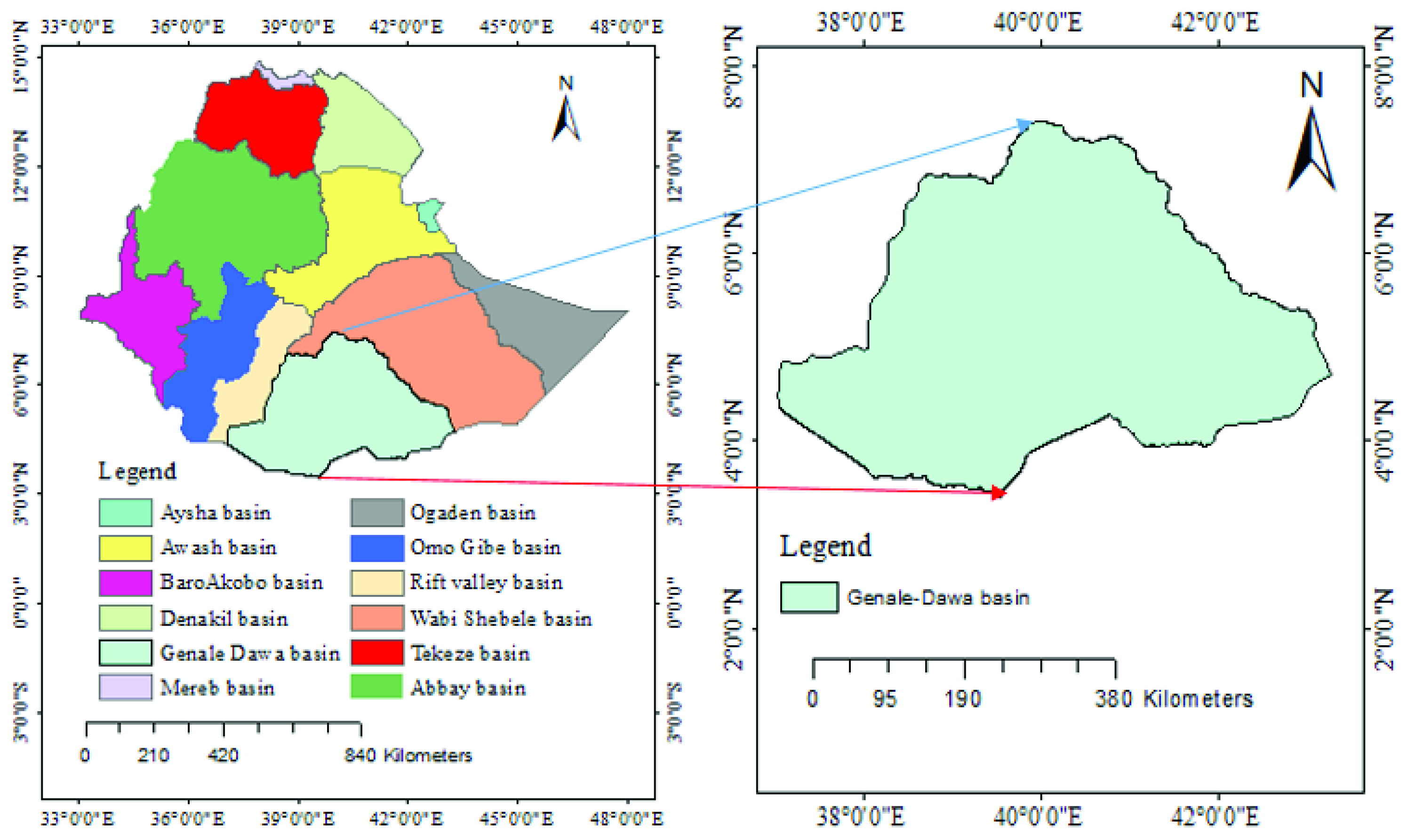
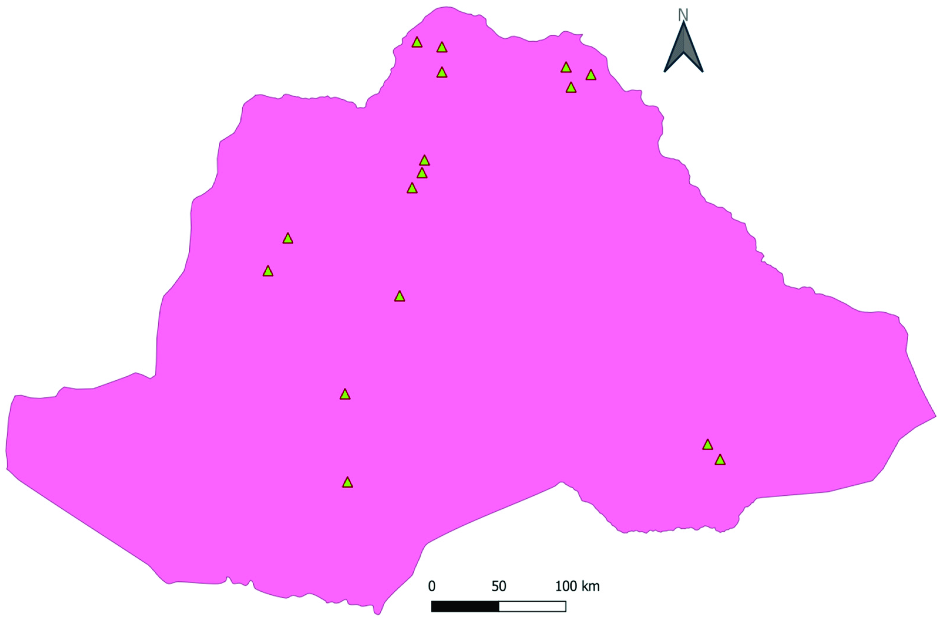
2.1. Description of the Study Area

The Genale–Dawa River Basin (GDRB) is the southernmost basin in Ethiopia, covering the western half of Bale and the southeastern, southwestern, and northeastern parts of Sidama and Somali regional states; it is geographically located (Figure 1) between 3°30′, 7°20′ north latitude and 37°05′, 43°20′ east longitude, covering 171,050 km². The basin comprises ~13.87% of the country’s total area, and is characterized by great geographical diversity, with high and rugged mountains, flat-topped plateaus, deep gorges, and plains.

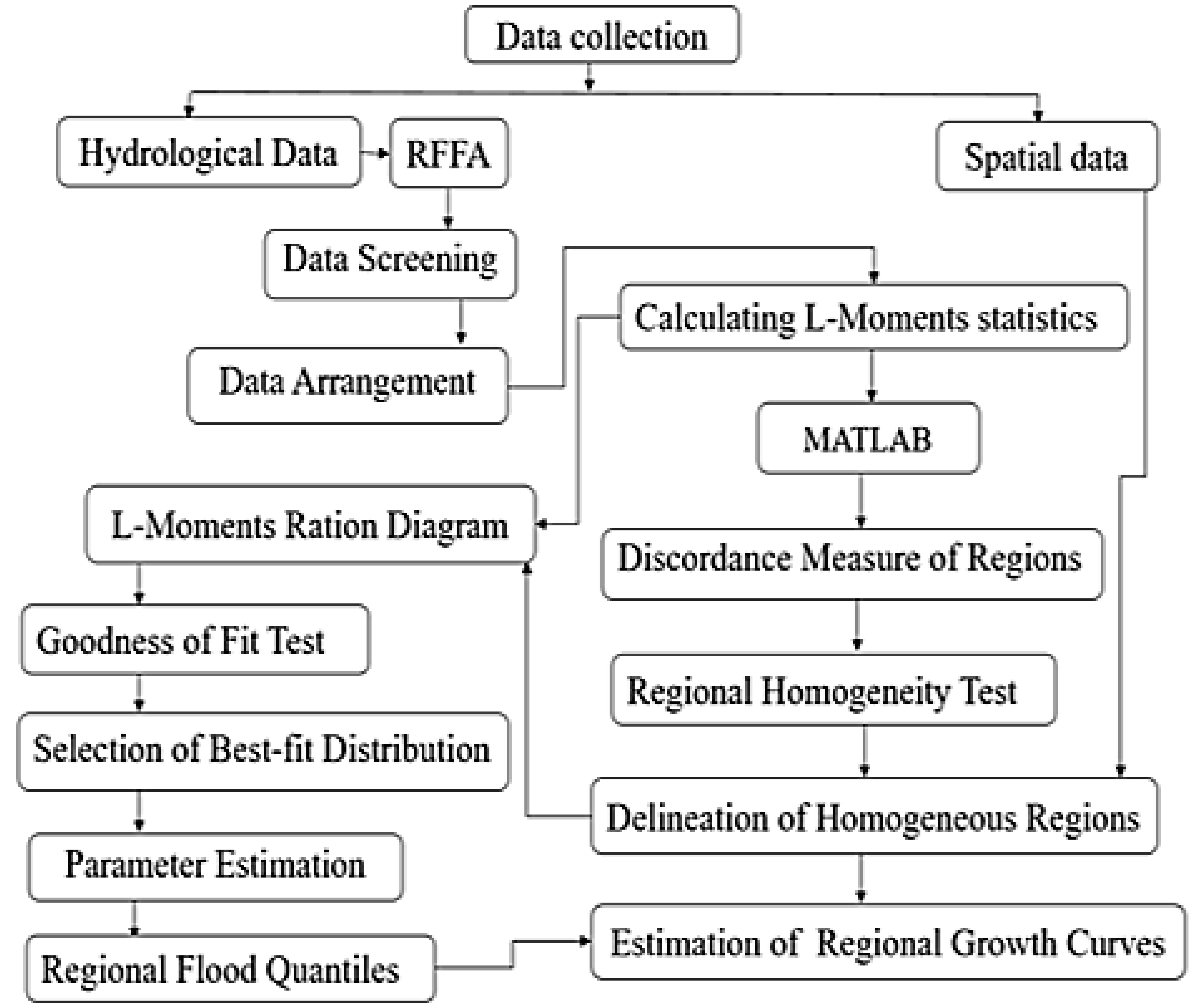
2.2. Screening, Sources, and Analysis of Data

The input proxy data layers were generated from remotely sensed satellite images with a digital image-processing algorithm and existing data. Flood frequency analysis primarily uses annual maximum flood data at gauging stations. Screening of data is the first step in regional flood frequency analysis [41], in which the engaged methods filter undesirable data series and sites from the study. This is used to check whether the data fit for the execution of regional research. The hydrological and digital elevation model (DEM) data were collected from the Ethiopian Water Irrigation and Electricity Ministry. DEM data were an essential input for delineating and specifying the location of the gauging stations in the basin. The site characteristics of stations for this study are as indicated in

Table 1. The site characteristics of gauging stations used in detailed analysis.

River	Location	Coordinate		Area (Km2)	Record Period	Time
		Latitude	Longitude			(Years)
Dawa	Melka Guba	4°52′	39°19′	19,611	1986–2015	30
Dawa	Near Digatty	4°17′	39°20′	12,710	1997–2015	19
Awatta	Near Odo Shakiso	5°54′	38°56′	1611	1997–2014	18
Genale	Chinamasa	5°31′	39°41′	10,574	1985–2008	24
Genale	Halwey	4°26′	41°50′	54,093	1985–2009	25
Genale	Kolle Bridge	4°32′	41°45′	83,219	1998–2008	13
Halgol	Near Gom-Goma	6°20′	39°50′	160	1990–2008	19
Mormora	Near Megado	5°41′	38°48′	1375	1985–2015	31
Shaya	Near Robe	7°10′	39°58′	433.8	1985–2014	30
Togona	Shallo Village	7°0′	39°58′	336.2	1985–2008	24
Weyib	Near Agarfa	7°12′	39°48′	7719	1985–2008	24
Weyib	Alemkerem	6°59′	40°58′	3576.9	1990–2009	20
Weyib	Near Denbel	7°2′	40°48′	1215	1986–2008	23
Weyib	Sofumer	6°54′	40°50′	3792.7	1990–2010	21
Welmel	Melka Amana	6°14′	39°46′	1048	1990–2009	20
Yadot	Near Dello Mena	6°25′	39°51′	531	1990–2008	19

. Accordingly, 16 gauging sites that satisfied the minimum of 10 years of records were carefully chosen for analysis. The minimum and maximum length of the at-site flood data records were 13 and 31 years, respectively. For all of the stations listed in

Table 2. Preliminary identified homogeneous regions for specific gauging sites.

Group Name	Station Name	Best Fit Distribution
Region-A	Chinamasa	GEV
	Kolle Bridge	GEV
	Halwey	GEV
	Melka Amana	GEV
	Gom-Goma	GEV
	Dello Mena	GEV
Region-B	Melka Guba	LPIII
	Megado	LPIII
	Digatty	LPIII
	Odo Shakiso	LPIII
Region-C	Robe	GPA
	Agarfa	GPA
	Shallo Village	GPA
	Alemkerem	GPA
	Denbel	GPA
	Sofumer	GPA

and shown in Figure 2, the flood data were later subjected to investigative data analysis in the study area. Based on the ability to achieve the predetermined objectives, ArcGIS10.4.1 delineates representative gauging stations and hydrologically homogeneous regions for the actual results. MATLAB2017a coding was employed to determine the discordancy of sites from the identified areas and plot regional growth curves. The general flowchart of the methodology was as indicated in Figure 3.

2.3. Hydrological Regionalization

Regionalization techniques are a vital option to address the shortage of streamflow data and provide sufficient flood control estimates. This is essential to estimate growth curves and peak flood quantiles for the tail of the frequency distribution [57]. The statistical values of flood statistics for the stations were checked using L-moments to see whether they could be classified under single or more regions. L-moments can give a balanced estimation, and cannot be easily biased by the presence of outliers [33,44,52,58]. Identification of similar regions is an extensive stage in hydrological regionalization; this is usually the most challenging stage, requiring the greatest number of significant decisions. This technique considers that the gauging stations were grouped into geographically continuous sites; the response of streams to physiographic variables should be similar. A DEM size of 30 m × 30 m was used to identify the site characteristics of the basin. Thus, the grouping of stations into a specific category was achieved by looking at stations’ site characteristics; then, stations with nearly the same site characteristics were clustered in the same region.

The method of L-moment ratio diagram (LMRD) is used as a means to give priority for identification of homogeneous regions and distributions based on the statistical principles. According to [29,36,51,52], the main suggestion of the LMRD is that if the maximum annual flows of dissimilar stations come from similar distribution, they form an identical region. This is a valuable way of representing the moments of different distributions depending on the statistical nature of the data. L-moment statistics are used to group stations in terms of geographical proximity and continuity of gauging stations. To use the statistical parameters, LCs and LCk are first computed. Those closely fitted stations are supposed to come from the same parent distribution, and are considered to belong to the same region and then tested with different homogeneity tests.

2.4. Discordancy Measure

The discordancy index (D_i) for sites in a region constitutes points in the three-dimensional space of sample L-moment ratios (LC_V, LCs, and LCk), as shown in [2]. The critical values D_i represent numbers of sites in a region at a significance level of 10%, as presented in [2]. These were used to assess each study site and identify whether they should be analyzed further to ensure homogeneity. If a vector, $U_i={\left({\mathsf{\tau }}_2^i,{\mathsf{\tau }}_3^i,{\mathsf{\tau }}_4^i\right)}^T$, which controls the L-moment ratios for site i, T is the transpose of the vector U_i. The discordancy measure of regions was tested and defined as follows:

$$D_i=\frac{1}{3}\left(U_i-{\overline{U}}_i\right)S^{-1}({\left(U_i-{\overline{U}}_i\right)}^T$$

(1)

$${\overline{U}}_i=\frac{1}{N}{\displaystyle \sum }_{i=1}^N{U}_i$$

(2)

$$S=\frac{1}{\left(N-1\right)}{\displaystyle \sum }_{i=1}^N(U_i-{\overline{U}}_i){\left(U_i-{\overline{U}}_i\right)}^T$$

(3)

where N is the total number of sites, D_i is the discordancy index, U_i is defined as a vector containing the L-moment ratios for site i, ${\overline{U}}_i$ is the group average of U_i, and S is the sample covariance matrix of U_i.

In this study, D_i is compared with the annual maximum flood series (AMF) of the 16 stream gauge stations in the GDRB to determine the relevance of the data used in the RFFA. The discordance index (D_i) values for different locations within the regions were calculated using MATLAB2017a, and are presented in

Table 3. Streamflow statistics for discordance tests and regional homogeneity tests.

Name of Station	LCv	LCs	LCk	Cv	Cs	Ck	Di
Region-A
Chinamasa	0.1999	0.0467	0.1142	0.3767	0.7377	1.3105	1.0313
Kolle Bridge	0.1386	0.0221	0.1017	0.2409	0.2473	−0.1652	1.1287
Halwey	0.2008	0.0893	0.0106	0.3457	0.3285	−1.2458	1.3149
Melka Amana	0.2079	−0.0830	−0.0070	0.3559	−0.2569	−1.1165	0.856
Gom-Goma	0.2575	0.0757	0.0285	0.4281	0.2689	−0.8923	0.9737
Dello Mena	0.2399	−0.0462	−0.0420	0.4025	−0.1339	−1.3512	0.6953
CC	0.1977			0.1814
Region-B
Melka Guba	0.2205	0.0750	0.0376	0.3900	0.3613	−0.5180	0.9999
Megado	0.2014	0.1444	−0.0181	0.3537	0.4413	−1.2430	0.9999
Digatty	0.1571	0.2078	0.2027	0.2891	0.9800	0.5214	0.9999
Odo Shakiso	0.1420	0.1718	0.2330	0.3117	0.2892	−1.1837	0.9999
CC	0.2043			0.1332
Region-C
Robe	0.1467	0.1152	0.1015	0.2864	0.3858	−0.5594	1.3966
Agarfa	0.2463	0.0904	−0.0704	0.4151	0.1876	−1.4661	1.5528
Shallo Village	0.1440	0.0074	0.0706	0.2424	−0.0296	−0.9363	0.6659
Alemkerem	0.1202	−0.2746	0.1009	0.2109	−0.9492	0.1508	0.5846
Denbel	0.1458	−0.0479	−0.0317	0.2303	−0.2159	−1.0681	0.5881
Sofumer	0.1458	−0.1523	−0.0428	0.2521	−0.4272	−1.2117	1.2120
CC	0.2806			0.2714

for the three regions. An appropriate standard to classify a station as discordant is if D_i ≥ 3. According to [54], a site is declared to be unusual if D_i is large.

2.5. Tests for Homogeneity of Stations and Regions

After a homogeneous region was identified, the degree of similarity of the aspirant region in terms of flow statistics was tested using L-moments. It was necessary that the region be satisfactorily homogeneous. No further division of the area into individual sites would improve the accuracy of flood estimates. The main benefit of L-moments is that they are a linear combination of data, are not influenced by outliers, and constitute unbiased model estimates [58]. Unbiased model estimators of the first four probability-weighted methods are recommended in [2]. The authors of [14,20,28,44,47] suggested a homogeneity test based on L-moments, which is possible. Different methods are available to inspect regional homogeneity in terms of the hydrological response of the stations. In this study, Cv- and LCv-based statistical homogeneity tests were applied to verify the acceptability of clustering techniques.

2.5.1. Conventional Homogeneity Test

The criterion used to check for regional homogeneity was based on the value of CC. The higher the values of Cv and CC, the lower the performance of the index flood method for the region under consideration. Hence, CC should be kept low for better confirmation of the index flood method [24,40]. The techniques used in this method to compute CC values are described below. The mean, standard deviation, and coefficient of variation were calculated for the delineated regions, as was the mean AMF of the station. The mean of AMF of the station was calculated as follows:

$${\overline{Q}}_i=\frac{1}{n}.{\displaystyle \sum }_{i=1}^n{Q}_i$$

(4)

The standard deviation of the AMF of the station:

$${\delta }_i=\sqrt{{\displaystyle \sum }_{i=1}^n\frac{{\left(Q_i-{\overline{Q}}_i\right)}^2}{n}}$$

(5)

$$C{v}_i=\frac{{\delta }_i}{{\overline{Q}}_i}$$

(6)

where Q_i is the flow rate in the region (m³/s) at site i, ${\overline{Q}}_i$ is the mean flow rate for the region (m³/s) at site i, $\delta i$ is the standard deviation for the region at site i, n is the number of the record year, and $C{v}_i$ is the coefficient of variation of a region at site i.

For each region, the corresponding CC value is calculated using the following relations:

Regional mean:

$${\overline{Cv}}_i=\frac{1}{N}.{\displaystyle \sum }_{I=1}^{N}C{v}_i$$

(7)

Regional standard deviation:

$${\delta }_c=\sqrt{\frac{{{\displaystyle \sum }}_{i=1}^N{\left(C{v}_i-{\overline{Cv}}_i\right)}^2}{N}}$$

(8)

The weighted regional Cv_i of all the sites, CC, is defined as follows:

$$CC=\frac{{\delta }_{Cv}}{{\overline{Cv}}_i}<\left(0.3\right)$$

(9)

where N is the number of the site in a region, ${\overline{Cv}}_i$ is the mean coefficient of the site’s Cv_i values, and $\delta Cv$ is the standard deviation of the site’s Cv_i values.

2.5.2. L-moment-Based Homogeneity Testing

L-moment-based homogeneity testing (LC_V) is a more accurate and effective way of testing the homogeneity of the site when compared with that of the C_v-based homogeneity test. The procedural calculation is the same as that of the C_v. The following are benefits of LC_v compared to C_v: LC_v can characterize a wide range of distribution, sample estimates are so robust that outliers in the dataset do not affect them, and they are less biased in estimation, yielding a more accurate estimate of the parameters of a fitted distribution [14,24,59]. The author [40], gave the unbiased estimators of ${\beta }_{0,} {\beta }_1,{\beta }_2,$ and ${\beta }_3$ as follows:

$${\beta }_0=\frac{1}{n}{\displaystyle \sum }_{i=1}^n{Q}_i$$

(10)

$${\beta }_1={\displaystyle \sum }_{i=1}^{n-1}\frac{\left(j-1\right)\left(Q_i\right)}{n\left(n-1\right)}$$

(11)

$${\beta }_2={\displaystyle \sum }_{i=1}^{n-2}\frac{\left(j-1\right)\left(j-2\right)\left(Q_i\right)}{n\left(n-1\right)\left(n-2\right)}$$

(12)

$${\beta }_3={\displaystyle \sum }_{i=1}^{n-3}\frac{\left(j-1\right)\left(j-2\right)\left(j-3\right)\left(Q_i\right)}{n\left(n-1\right)\left(n-2\right)\left(n-3\right)}$$

(13)

where $Q_i$ is the annual maximum flow (m³/s) from the station’s dataset, n is the number of years, j is the rank, and ${\beta }_o, {\beta }_1, {\beta }_2,\mathrm{and}{\beta }_3$ are L-moments estimators.

The first few moments are as follows:

$${\lambda }_1={\beta }_O$$

(14)

$${\lambda }_2=2{\beta }_1-{\beta }_O$$

(15)

$${\lambda }_3=6{\beta }_2-6{\beta }_1+{\beta }_O$$

(16)

$${\lambda }_4=20{\beta }_3-30{\beta }_2+12{\beta }_1-{\beta }_O$$

(17)

Specifically, λ₁ is the mean of the distribution or measure of location, λ₂ is a measure of scale, τ₃ is a measure of skewness, and τ₄ is a measure of kurtosis. L-skewness and L-kurtosis are defined relative to the L-scale, λ₂; sample estimates of L-moment ratios can be written as LCv, LCs, and LCk [44]. A region that confidently satisfies all criteria for being hydrologically homogeneous can be derived. L-moment ratios are independent of units of measurement, and are given as described in [2], as follows:

$${\tau }_2=\frac{{\lambda }_2}{{\lambda }_1},{\tau }_3=\frac{{\lambda }_3}{{\lambda }_2},{\tau }_4=\frac{{\lambda }_4}{{\lambda }_2}$$

(18)

Using the above procedural formula,

$${\overline{L}}_{Cvi}=\frac{1}{n}.{\displaystyle \sum }_{i=1}^N{L}_{Cvi}$$

(19)

$${\delta }_{Cv}=\sqrt{{\displaystyle \sum }_{i=1}^n\frac{\left(L_{Cvi}-{\overline{L}}_{Cvi}\right)}{n-1}}$$

(20)

The weighted regional L_CVi of all the sites, CC, is defined as follows:

$$CC=\frac{{\delta }_{LCv}}{{\overline{CV}}_i}<\left(0.3\right)$$

(21)

2.6. Delineation of Homogeneous Regions

The delineation of similar regions relates to the identification of regional distributions [24]. In this study, the DEM of the GDRB was used to delineate homogeneous areas by taking into account the drainage boundaries of the sub-basin with the ArcGIS 10.4.1 environment. Homogeneity tests were used to check the clustered regions, and all stations were positioned with latitude and longitude. For each station, the statistical values of LCs and LCk were calculated and measured linearly.

2.7. Selection of Regional Distribution

Regional distribution was determined based on goodness-of-fit measures, which direct which distribution fits the available data. In this analysis, annual maximum flow corresponding to a given return period can be predicted using various theoretical distributions [37,38,47,51,55,59,60]. In this study, the L-moment ratio diagram (LMRD) was used to select the best fit probability distribution. LMRD is an appropriate way of representing candidate distributions as the plot of LCs versus LCk, as described in [44,46,47,52,57,61]. This popular and widely accepted method is used to identify and select distribution for the sub-basin. Acceptable techniques are needed in order to select a model that reduces uncertainties in flood estimation. Distribution fitting using LMRD is highly dependent on regional mean weighted L-moment statistical values of LCs and LCk for all sites in the defined homogeneous regions. This shows the grouping of the datasets around the theoretical relationships between LCs and LCk of dissimilar probability distributions. Thus, acceptable design procedures are essentially required in order to indicate a model that minimizes uncertainties. Several flood frequency distributions have been practiced for modeling, but none has been universally accepted [2,52,62]. Generalized extreme value (GEV), generalized logistic (GLO), logistic, generalized Pareto (GPA), normal, log-Pearson type 3 (LPIII), and log-normal (LN) distributions are among the employed distributions in this study. Hence, these distributions were considered to represent the average distribution of the regional data of the basin.

A robust distribution should produce reasonably reliable estimates. Averages of L-skewness and L-kurtosis within a homogeneous region can be plotted on LMRDs along with theoretical curves for various candidate distributions. The nearest distribution should be a proper selection for the parent distribution in the region [19,59,63]. The distances separating group samples points from the curve for a specific distribution can be assumed to measure the goodness of fit. The graphical choice of distribution using LMRDs depends on the homogeneity of regional data [38]. LMRDs were used to make an initial choice of candidate distributions for the sub regions in this study. This is because the LMRDs can compare the fit of several distributions at once using a graphical tool. In using the LMRDs, sample L-moment ratios were compared to the population ones via the LMRD to obtain the best fit distribution for representing the sample data, providing a graphical judgment of L-moments; this involves plotting the L-moment ratios as a scatterplot and comparing them with the L-moment ratio points of the candidate distributions.

Comparing the results of the flood events over a 10,000-year return period is significant. This is because the dam safety risk analyses, the sizing of emergency spillways, the design of dam crest level and any other hydraulic structures, and the critical flood peaks are the main criteria of the 10,000-year flood return period [56,64]. This may help to make balanced engineering decisions on the choice of design floods used to ensure a satisfactory and reliable standard in the planning and design of flood control structures. The simulated dimensionless quantile estimates for each site and the region were calculated; it was then possible to get flood estimates for each site by multiplying the dimensionless quantiles by the sample means of each site. The more robust distribution is usually used for the RFFA when two or more distributions are acceptable to the regional data. Stations with computed values of scale, location, and shape parameters can determine the quantile with different return periods using other equations for various distributions. For GEV distribution, the flow quantile can be estimated as follows:

$$X_T=\mu +\frac{\delta }{k}\left(1-\left(-ln{\left(1-\frac{1}{T}\right)}^k\right)\right),\mathrm{for}k\ne 0$$

(22)

For GPA distribution, the flow quantile can be estimated as follows:

$$X_T=\mu +\frac{\delta }{k}\left(1-{\left(\frac{1}{T}\right)}^k\right),\mathrm{for}k\ne 0$$

(23)

where $\delta$ is the scale parameter, T is the return period, $\mu$ is the location parameter, and $k$ is the shape parameter.

The curve of the mean of sites’ growth was used to represent the frequency curve of regions. In this study, the index flood method utilized data of the gauged catchments to evaluate the regional correlation between the flood magnitudes of various return periods for the assessment of ungauged catchments [19,34,63]. The model parameters for the distributions for each station were used to calculate consistent flow estimates conforming to the return periods of 2–10,000 years. Regional growth curves were derived and generated by plotting Q/Q_m versus the Gumbel reduced variate (−ln (−ln(1 − 1/T)).

3. Results and Discussion

3.1. Identification of a Homogeneous Region

The homogeneity of the group with respect to extreme flow statistics had to be tested. The degree of homogeneity of a region was proposed based on site characteristics and the LMRD of flood statistics. The grouping of sites was carried out by cogitating geographically continuity (spatial proximity on the network of gauging stations) as the initial point, as shown in Figure 2. In clustering, the maximum flow of sites in the region should satisfy the homogeneity test criteria given in [2]. LMRD was then used to group stations to confirm the priority clustering. As indicated in Table 2, the accentuated distributions were designated to the same groups, since the stations lay close to the same distributions assigned as Region-A, Region-B, and Region-C, as shown in Table 2. Hence, three homogeneous subregions were identified based on L-moment statistics and the suitability of gauging site networks. The L-moments approach is a classic technique of hydrological homogeneity analysis, used by various researchers worldwide to obtain more consistent assessments with probability distributions in RFFA [39,41,42,46,63]. For this study, the L-moments approach was used as a tested criteria of the basin’s regional homogeneity [16].

3.2. Discordancy Measure

This approach was used to validate the defined regions and screen the data from unusual sites. The discordancy measure (D_i) for each site in the sub-basin is indicated in Table 3. All were less than the critical value of 2.491 for 10 locations, as shown in [2]. This suggests that all of the stations within the sub-basin satisfied the discordance test criteria. Hence, none of the sub-basin gauging stations was more significant than the critical value. This indicates that there were no unusual sites in the sub-basin. It was noted that the D_i values for all sites varied from 0.5846 to 1.5528. The critical values of the discordancy index D_i for various numbers of sites in a region at a significance level of 10% were obtained from [2]. A site is confirmed to be unusual if D_i is large in this condition; this would be considered entirely discordant, justifying the removal of sites from the defined regions, and can be redefined as a single site or fused into other regions. Hence, all of the stations grouped as homogeneous in Region-A, Region-B, and Region-C satisfied the discordance test criteria. According to [14,33,36,41,44,47,52,58,59,63], the regions under investigation were homogeneous if D_i was less than 3. As shown in Table 3, the D_i result was below the critical value, implying that all of the regions were homogeneous; thus, none of the identified areas revealed D_i greater than the critical value. This indicates that not all of the sites reflect outliers and discordancy.

3.3. Test for Regional Homogeneity

The streamflow statistical values identified in homogeneous regions have to be statistically homogeneous in order to verify their acceptability. Here, the internal homogeneity of regions was determined based on flow statistics. For better performance of the index flood method, the combined coefficient of variation (CC) should be kept low [24,58]. The combined coefficient of variation (CC) values for the region were calculated. The results in sites of each area were summarized as shown in Table 3. The value of CC varies from region to region, depending on flow data. In the Cv-based homogeneity test, the CC values were 0.1814, 0.1332, and 0.2714 for Region-A, Region-B, and Region-C, respectively. On the other hand, in the LCv-based homogeneity test, the CC values were 0.1977, 0.2043, and 0.2806 for Region-A, Region-B, and Region-C, respectively. A region was confirmed to be homogeneous if it was geographically contiguous [23,24,37,52,60,65]. Hence, for the better performance of the index flood method, CC should be kept low and small. Moreover, other authors, such as [58], note that a region can be affirmed to be homogeneous for the study region(s) under consideration if the CC value is less than 0.3. All regions were hydrologically homogeneous for Cv- and LCv-based homogeneity tests, since their CC values were less than 0.3, as shown in Table 3. As a result, it can be concluded that all regions in the GDRB were reasonably homogeneous.

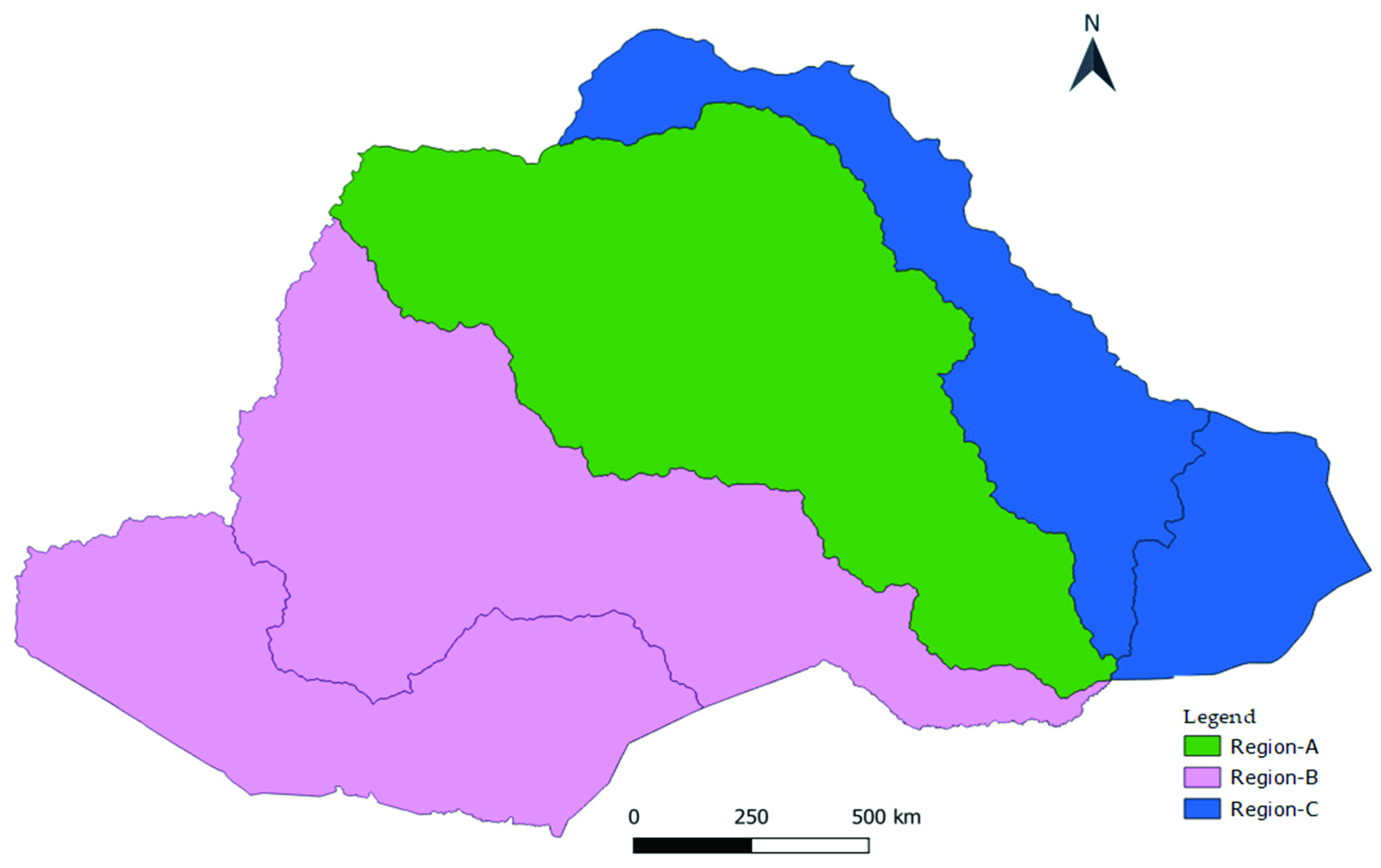
3.4. Demarcation of Homogeneous Regions

Delineation of regions was carried out because the statistical homogeneity tests were satisfied and proved wholly discordant. The regions covered areas of 56,343, 83,250, and 32,666 km² for Region-A, Region-B, and Region-C, respectively. This implies that 32.708, 48.328, and 18.963% of the basin is delineated under Region-A, Region-B, and Region-C, respectively. Having proven to be statistically homogeneous, the regions shown in Figure 4 could generate a regional growth curve at any site located in the study area. The delimitation of homogeneous regions is the most significant and exciting step in RFFA [25,37,41,59,66,67]. Various studies worldwide have developed regionalization techniques intended to create homogeneous areas, and applied probability distributions in RFFA as the most effective approach [2,16,32,37,38].

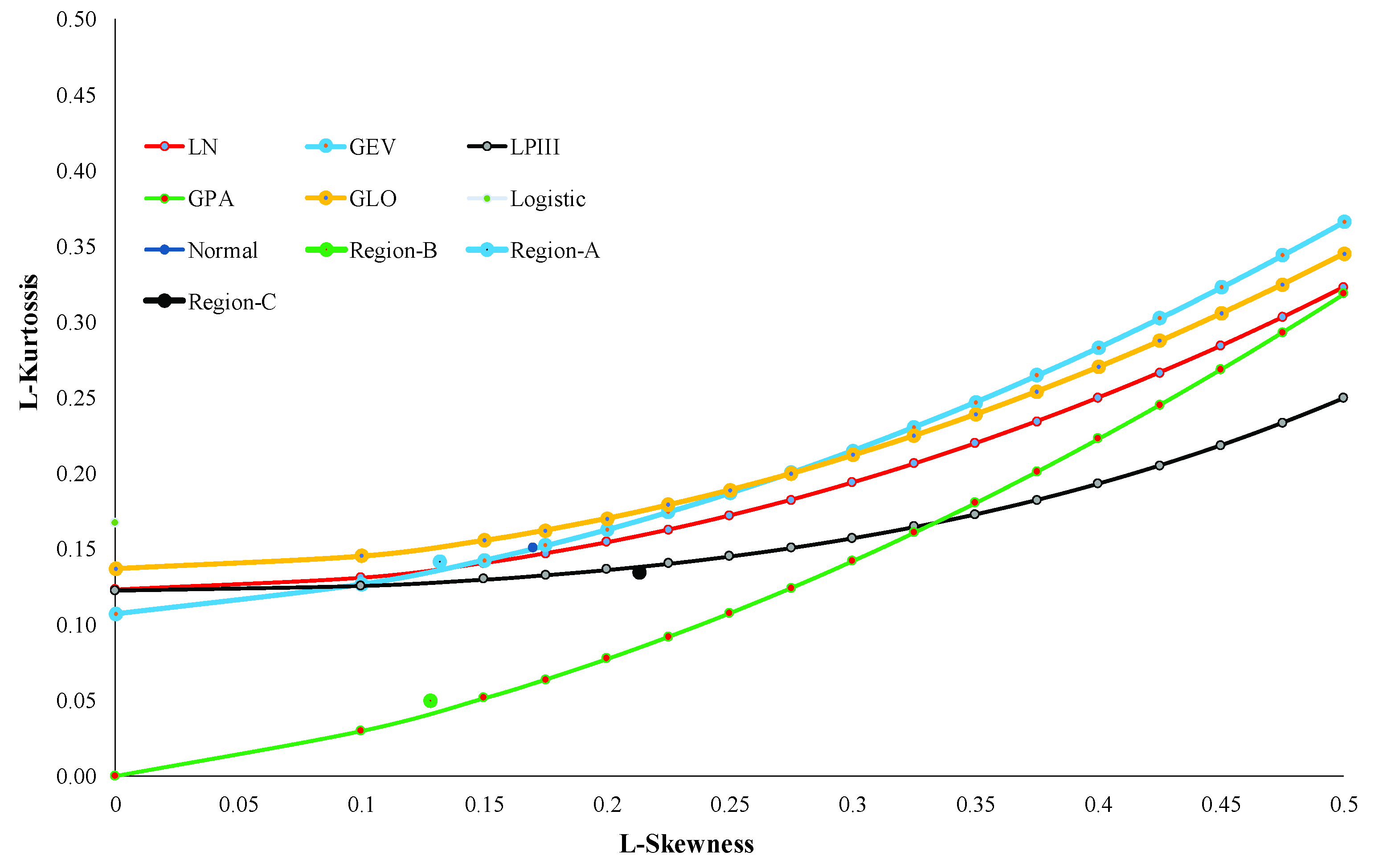
3.5. Selection of Best Fit Distribution

The corresponding average weighted values of L-moment statistics results were obtained from regional data as presented in Table 3, plotted along the theoretical lines for some distributions on LMRDs to determine a regional probability distribution. The points representing the regional average values of L-kurtosis versus L-skewness were fitted with LPIII, GPA, and GEV distributions, as shown in Figure 5. The record length’s weighted average proximity to a candidate distribution’s theoretical curve or position in L-skewness, L-kurtosis space was used to highlight the distribution’s suitability for defining regional data. The adequacy of a candidate distribution to describe regional data was shown by the resemblance of a line of best fit to the theoretical curve of that distribution in L-skewness, L-kurtosis space. Therefore, it appears that the LPIII, GEV, and GPA distributions were accepted as governing regional distributions in the GDRB to estimate regional floods for the three regions. LPIII is a statistical method of fitting frequency distribution values for predicting floods at a few areas of a specified river. A mathematical model of GEV, GPA, and LPIII frequency distribution was constructed by manipulating data statistics at a particular river site for maximum flood discharge, and a return period was developed for flood frequency analysis [21,68,69,70]. Other similar conclusions of a positive linear relationship between the dimensionless index flood and the GEV reduced variate were found by [10,52]. Studies indicate different degrees of accuracy in estimating flood quantiles.

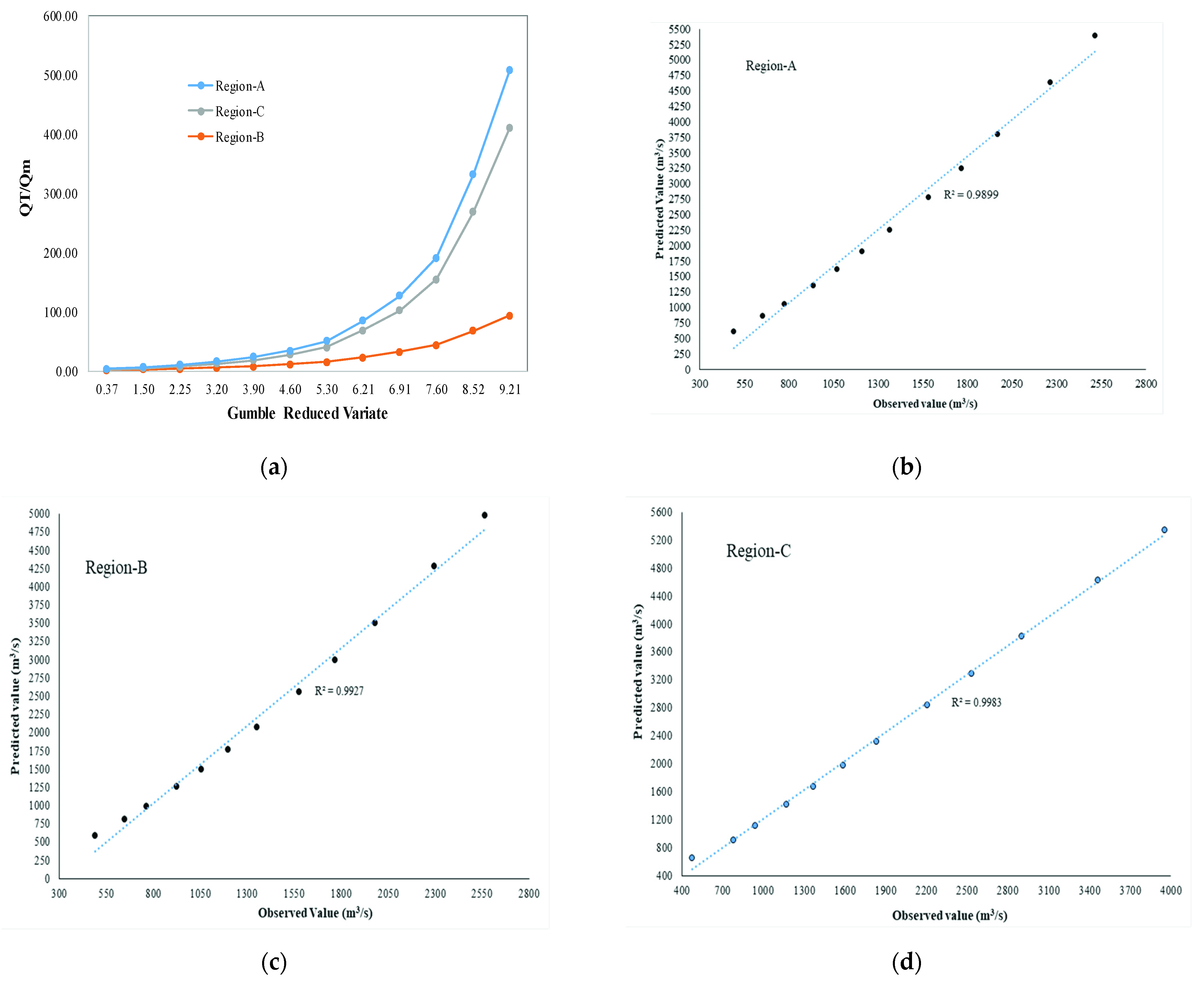
3.6. Performance Evaluation of Regional Flood Frequency Analysis

The performance of the regional L-moments algorithm depends on particular criteria used to measure the performance of estimators [68]. After regions were accepted as homogeneous, suitable distributions were identified for the areas. Index flood methods consider that the statistical nature of the selected gauging stations in a region is the same after scaling with the index flood value. This technique utilizes the data of the gauged catchments to evaluate regional relationships, based on which the flood magnitudes of various returns for ungauged catchments can be assessed. After the regional frequency distribution is determined, the flood quantile with a T-year return period within the sub-basin can be estimated. The common practice is to obtain the dimensionless data to divide the estimate of the at-site mean. Parameters of the distribution of X_T can be found from the combined set of regional data.

Analytical goodness-of-fit criteria are helpful to determine whether the elimination of particular data from the model is statistically significant or not. This implies that the frequency distributions chosen as the best distribution could fit regional flood models for the basin. For this analysis, the performance of the best distribution model for the respective regions was evaluated, comparing predicted with observed peak flood quantile plots, as shown in Figure 6b–d, indicating that almost all plots were well fitted to the line. These plots were used to compare the estimated quantiles and the observed flood values, as well as to check the validity of the estimates provided by a fitted theoretical distribution. Through all of the patterns, we found that the GEV, GPA, and LPIII distributions performed well for Region-A, Region-B, and Region-C in the GDRB. The flood quantile estimates based on the predicted peak flood quantiles were consistent with the flood quantile estimates based on the observed peak flood quantile data. The correlation (R²) coefficients were 0.9899, 0.9927, and 0.9983 for Region-A, Region-B, and Region-C, respectively; this indicates that the predicted peak flood quantile shows good agreement with the observed peak flood quantile. From Figure 6b–d, it can be observed that the R² values of predicted and observed peak flood quantiles plotted for the three regions were close to 1, showing the strongest correlation between the parameters and the validity of the applied RFFA in the study area; this implies that the developed scatterplots for observed and predicted flood quantiles are in good agreement. However, we observed that the relative error difference between the observed and predicted peak flood quantiles was high. There was uncertainty in the peak flood quantile estimates, as a perfectly homogeneous region is rarely attainable, and the distribution does not truly represent the pooled samples [51,64].

Moreover, quantile estimates are subject to sampling errors, as sample data estimate parameters that influence peak flood quantiles and large areas of the limited observed data [13,51,71]. The uncertainties in flood quantiles are due to the convolution of parameters during the prediction [64]. This might explain the overpredicted peak flood quantiles, although methods of L-moments are unbiased and do not suffer from sample-size-related limitations [72]. Some of the parameters that influence long-term recurrence intervals may not yield reasonable estimates, due to the variability of different physical processes and anthropogenic influences in the regions [39,52]. Better results can be attained by addressing variable input limitations [15,39,72]. This suggests that the index flood method produces higher errors in arid regions by overpredicting flood quantiles [68]. The selection of a frequency distribution in RFFA could lead to error and bias, particularly in higher return periods, resulting in overestimation of flood quantiles [56,64,73,74]; this results in a high probability of flooding, leading to loss of life and property [13,35]. Conversely, this can lead to large outlet structure design if used for design purposes, resulting in unreliable project costs [56,64]. Estimation of quantiles in a frequency distribution is governed by index flood variability, which is not addressed by index-flood-based regional L-moments algorithms [16,35]. Hence, the regionalization technique should be applied along with other physical catchment features, such as basin physiography and climatic characteristics, in order to improve the analysis and provide flood quantile estimates at gauged and ungauged sites [21,26,46,52].

The regional growth curve for the region was estimated after the region’s homogeneity was tested and the proper regional best fit frequency distribution was selected. The estimated growth curves are shown in Figure 6a. The higher deviations of regional curves may be due to the considerable spatial fluctuations of elevations with the spatially undulating topography of the basin. The regional standardized flood quantile for various return periods was predicted based on selected best fit distributions using the index flood method and growth curves, as depicted in Figure 6a. The flood frequency curves for each station were derived based on the proper distribution for various return periods. As a result, the selected distributions could be adopted as appropriate, and were found to be the dominating distributions in the GDRB for accurate evaluation and estimation of floods. The measurement of flood quantiles was applied for a 2–10,000-year return period [56]. From Figure 6a, it can be observed that the magnitude of flooding increases as the return period increases for selected distribution parameters in the three regions. This indicates that the growth curves of Region-A cause flooding in its lower reaches, facing high flood generation from the highlands. In addition, the Genale River might submerge low-lying areas in their outlets. Therefore, the lower reaches of homogeneous Region-A might be affected by flooding.

The growth curves of Region-B indicate a similar flooding problem in its lower reaches, suffering high flood generation from the highlands of the Awata sub-watershed. The flooding from the highlands might submerge the lower reaches of the sub-watershed; hence, this region’s middle and lower reaches are susceptible to the risk of flooding. Generally, Figure 6a reveals that lower elevation catchments have lower flood values but higher extreme flood variability than higher elevation catchments. The constructed regional curves from the three regions reflect the fact that all curves have different flood characteristics. This could be because the flooding in the various areas has different flood statistics. Furthermore, as indicated in Figure 6a, Region-C’s derived regional growth curve reveals higher quantile estimates than those of Region-A and Region-B for the same return periods. This high flooding within the region might cause tremendous damage and disruptions to local communities. This could be attributed to the variability in the flood management of the study basin. Therefore, our results confirm that the flood frequency of the regions was well addressed. Hence, using these distributions and annual maximum flow modeling could have a wide range of applications in agriculture, hydrology, engineering design, and future climate evaluation in the study area.

4. Conclusions

This study was performed using the data of 16 stream gauging stations to ensure reliable regional flood estimation in the Genale–Dawa River Basin for sustainable water resource management using the index flood and L-moments approach. The basin was defined and delineated into three hydrologically homogeneous regions, named Region-A, Region-B, and Region-C. Regional homogeneity and discordancy of the sites were used to verify the homogeneity of regions. All regions showed acceptable results for the discordancy index and statistical homogeneity tests using MATLAB and L-moments statistics. Thus, the L-moments method was found to be suitable for streamflow-based regionalization of the study area. Goodness-of-fit tests based on the L-moments ratio diagram were applied and found to be ideal for checking the adequacy of fitting an appropriate distribution for the recorded data of the basin. Generalized extreme value, log-Pearson type III, and generalized Pareto were identified as qualified distributions for Region-A, Region-B, and Region-C. Hence, the L-moments ratio diagram found an acceptable method for selecting the best fit distribution for estimating flood quantiles.

The derived regional growth curves were different for the three regions, confirming the heterogeneity of the areas. In addition, the derived results could be helpful as a reference in any hydrological considerations in the study area. This study found that delineation of homogeneous hydrological regions based on statistical parameters of gauged sites could be considered an acceptable method of regional analysis. We also confirmed the robustness of the L-moments-based index flood approach in identifying homogeneous regions. This method assigns a probability distribution to the regionally pooled groups in order to estimate the regional growth curve. This study consisted purely of statistical analysis using annual streamflow data, without considering other climatic variabilities and governing physics. Hence, the regionalization technique could be applied with other physical catchment features, such as basin physiography and climatic characteristics, in order to improve the analysis and provide flood quantile estimates at both gauged and ungauged sites. Hence, it is suggested that the established method should enhance testing under climate change scenarios to provide more reliable design flood estimates by applying hydraulic and hydrological models. The methodological outline of this study can be suitable for developing similar studies on river basins in other similar or different climatic zones.

References

1. Stedinger, J.R.; Griffis, V. Flood Frequency Analysis in the United States. J. Hydrol. Eng. 2008, 13, 199–204. [Google Scholar] [CrossRef] [Green Version]
2. Hosking, J.R.M.; Wallis, J.R. Regional Frequency Analysis: An Approach Based on L-Moments; Cambridge University Press: New York, NY, USA, 1997. [Google Scholar]
3. Kochanek, K.; Strupczewski, W.G.; Bogdanowicz, E. On seasonal approach to flood frequency modelling. Part II: Flood frequency analysis of Polish rivers. Hydrol. Process. 2012, 26, 717–730. [Google Scholar] [CrossRef]
4. Schendel, T.; Thongwichian, R. Considering historical flood events in flood frequency analysis: Is it worth the effort? Adv. Water Resour. 2017, 105, 144–153. [Google Scholar] [CrossRef]
5. Blöschl, G.; Bierkens, M.F.P.; Chambel, A.; Cudennec, C.; Destouni, G.; Fiori, A.; Kirchner, J.W.; McDonnell, J.J.; Savenije, H.H.G.; Sivapalan, M.; et al. Twenty-three unsolved problems in hydrology (UPH)—A community perspective. Hydrol. Sci. J. 2019, 64, 1141–1158. [Google Scholar] [CrossRef] [Green Version]
6. Machado, M.J.; Botero, B.A.; López, J.; Francés, F.; Díez-Herrero, A.; Benito, G. Flood frequency analysis of historical flood data under stationary and non-stationary modelling. Hydrol. Earth Syst. Sci. 2015, 19, 2561–2576. [Google Scholar] [CrossRef] [Green Version]
7. Lee, D.-H.; Kim, N.W. Regional Flood Frequency Analysis for a Poorly Gauged Basin Using the Simulated Flood Data and L-Moment Method. Water 2019, 11, 1717. [Google Scholar] [CrossRef] [Green Version]
8. Hassan, B.G.H.; Ping, F. Formation of Homogenous Regions for Luanhe Basin—By Using L-Moments and Cluster Techniques. Int. J. Environ. Sci. Dev. 2012, 3, 205–210. [Google Scholar] [CrossRef]
9. Javeed, Y.; Apoorva, K.V. Flow Regionalization Under Limited Data Availability—Application of IHACRES in the Western Ghats. Aquat. Procedia 2015, 4, 933–941. [Google Scholar] [CrossRef]
10. Hailegeorgis, T.T.; Alfredsen, K. Regional flood frequency analysis and prediction in ungauged basins including estimation of major uncertainties for mid-Norway. J. Hydrol. Reg. Stud. 2017, 9, 104–126. [Google Scholar] [CrossRef]
11. Lilienthal, J.; Fried, R.; Schumann, A. Homogeneity testing for skewed and cross-correlated data in regional flood frequency analysis. J. Hydrol. 2018, 556, 557–571. [Google Scholar] [CrossRef] [Green Version]
12. Nathanael, J.; Smithers, J.; Horan, M. Assessing the performance of regional flood frequency analysis methods in South Africa. Water SA 2018, 44, 387–398. [Google Scholar] [CrossRef] [Green Version]
13. Tanaka, T.; Tachikawa, Y.; Iachikawa, Y.; Yorozu, K. Impact assessment of upstream flooding on extreme flood frequency analysis by incorporating a flood-inundation model for flood risk assessment. J. Hydrol. 2017, 554, 370–382. [Google Scholar] [CrossRef]
14. Cassalho, F.; Beskow, S.; de Mello, C.R.; de Moura, M.M. Regional flood frequency analysis using L-moments for geographically defined regions: An assessment in Brazil. J. Flood Risk Manag. 2018, 12, e12453. [Google Scholar] [CrossRef]
15. Ekeu-wei, I.T. Evaluation of Hydrological Data Collection Challenges and Flood Estimation Uncertainties in Nigeria. Environ. Nat. Resour. Res. 2018, 8, 44. [Google Scholar] [CrossRef] [Green Version]
16. Malekinezhad, H.; Nachtnebel, H.P.; Klik, A. Regionalization approach for extreme flood analysis using L-moments. J. Agric. Sci. Technol. 2011, 13, 1183–1196. [Google Scholar]
17. Komi, K.; Amisigo, B.; Diekkrüger, B.; Hountondji, F. Regional Flood Frequency Analysis in the Volta River Basin, West Africa. Hydrology 2016, 3, 5. [Google Scholar] [CrossRef] [Green Version]
18. Ahn, J.; Cho, W.; Kim, T.; Shin, H.; Heo, J.H. Flood frequency analysis for the annual peak flows simulated by an event-based rainfall-runoff model in an urban drainage basin. Water 2014, 6, 3841–3863. [Google Scholar] [CrossRef] [Green Version]
19. Abida, H.; Ellouze, M. Probability distribution of flood flows in Tunisia. Hydrol. Earth Syst. Sci. 2008, 12, 703–714. [Google Scholar] [CrossRef] [Green Version]
20. Zhang, Q.; Gu, X.; Singh, V.P.; Sun, P.; Chen, X.; Kong, D. Magnitude, frequency and timing of floods in the Tarim River basin, China: Changes, causes and implications. Glob. Planet. Chang. 2017, 139, 44–55. [Google Scholar] [CrossRef] [Green Version]
21. Ibeje, A.O.; Ekwueme, B.N. Regional Flood Frequency Analysis using Dimensionless Index Flood Method. Civ. Eng. J. 2020, 6, 2425–2436. [Google Scholar] [CrossRef]
22. Seckin, N.; Haktanir, T.; Yurtal, R. Flood frequency analysis of Turkey using L-moments method. Hydrol. Process. 2011, 25, 3499–3505. [Google Scholar] [CrossRef]
23. Hassan, B.G.H.; Ping, F. Regional Rainfall Frequency Analysis for the Luanhe Basin—By Using L-moments and Cluster Techniques. APCBEE Procedia 2012, 1, 126–135. [Google Scholar] [CrossRef] [Green Version]
24. Gebregiorgis, A.S.; Moges, S.A.; Awulachew, S.B. Basin Regionalization for the Purpose of Water Resource Development in a Limited Data Situation: Case of Blue Nile River Basin, Ethiopia. J. Hydrol. Eng. 2013, 18, 1349–1359. [Google Scholar] [CrossRef]
25. Wiltshire, S.E. Grouping basins for regional flood frequency analysis. Hydrol. Sci. J. 1985, 30, 151–159. [Google Scholar] [CrossRef] [Green Version]
26. Ahn, K.-H.; Palmer, R. Regional Flood Frequency Analysis Using Spatial Proximity and Basin Characteristics. J. Hydrol. 2016, 540, 329–338. [Google Scholar] [CrossRef]
27. Bogdanowicz, E.; Kochanek, K.; Strupczewski, W.G. The weighted function method: A handy tool for flood frequency analysis or just a curiosity? J. Hydrol. 2018, 559, 209–221. [Google Scholar] [CrossRef]
28. Cassalho, F.; Beskow, S.; Vargas, M.M.; de Moura, M.M.; Ávila, L.F.; de Mello, C.R. Hydrological regionalization of maximum stream flows using an approach based on L-moments. RBRH 2017, 22, 2318–2331. [Google Scholar] [CrossRef]
29. Wu, Y.; Lall, U.; Lima, C.H.R.; Zhong, P. Local and regional flood frequency analysis based on hierarchical Bayesian model: Application to annual maximum streamflow for the Huaihe River basin. Hydrol. Earth Syst. Sci. Discuss. 2018, 12, 253–262. [Google Scholar] [CrossRef] [Green Version]
30. Odry, J.; Arnaud, P. Comparison of Flood Frequency Analysis Methods for Ungauged Catchments in France. Geosciences 2017, 7, 88. [Google Scholar] [CrossRef] [Green Version]
31. Cassalho, F.; Beskow, S.; de Mello, C.R.; de Moura, M.M.; Kerstner, L.; Ávila, L.F. At-Site Flood Frequency Analysis Coupled with Multiparameter Probability Distributions. Water Resour. Manag. 2018, 32, 285–300. [Google Scholar] [CrossRef]
32. Burn, D.H. Evaluation of Regional Flood Frequency Analysis with a Region of Influence Approach Evaluation of Regional Flood Frequency Analysis with a Region of Influence Approach. Water Resour. Res. 1990, 26, 2257–2265. [Google Scholar] [CrossRef]
33. Hussain, Z.; Pasha, G.R. Regional flood frequency analysis of the seven sites of Punjab, Pakistan, using L-moments. Water Resour. Manag. 2009, 23, 1917–1933. [Google Scholar] [CrossRef]
34. Kyselý, J.; Picek, J. Regional growth curves and improved design value estimates of extreme precipitation events in the Czech Republic. Clim. Res. 2007, 33, 243–255. [Google Scholar] [CrossRef]
35. Nobert, J.; Mugo, M.; Gadain, H. Estimation of design floods in ungauged catchments using a regional index flood method. A case study of Lake Victoria Basin in Kenya. Phys. Chem. Earth 2014, 67–69, 4–11. [Google Scholar] [CrossRef]
36. Noto, L.V.; La Loggia, G. Use of L-Moments Approach for Regional Flood Frequency Analysis in Sicily, Italy. Water Resour. Manag. 2009, 23, 2207–2229. [Google Scholar] [CrossRef]
37. Parida, B.P.; Kachroo, R.K.; Shrestha, D.B. Regional Flood Frequency Analysis of Mahi-Sabarmati Basin (Subzone 3-a) using Index Flood Procedure with L-Moments. Water Resour. Manag. 1998, 12, 1–12. [Google Scholar] [CrossRef]
38. Peel, M.C.; Vogel, R.M.; Mcmahon, T.A. The utility of L-moment ratio diagrams for selecting a regional probability distribution. Hydrol. Sci. Bull. 2001, 46, 147–155. [Google Scholar] [CrossRef]
39. Yang, T.; Xu, C.; Shao, Q.; Chen, X. Regional flood frequency and spatial patterns analysis in the Pearl River Delta region using L-moments approach. Stoch. Environ. Res. Risk Assess. 2010, 24, 165–182. [Google Scholar] [CrossRef]
40. Hosking, J.R.M.; Wallis, J.R. Some Statistics Useful in Regional Frequency Analysis. Water Resour. Res. 1993, 29, 271–281. [Google Scholar] [CrossRef]
41. Drissia, T.K.; Jothiprakash, V.; Anitha, A.B. Flood Frequency Analysis Using L Moments: A Comparison between At-Site and Regional Approach. Water Resour. Manag. 2019, 33, 1013–1037. [Google Scholar] [CrossRef]
42. Kumar, R.; Goel, N.K.; Chatterjee, C.; Nayak, P.C. Regional Flood Frequency Analysis using Soft Computing Techniques. Water Resour. Manag. 2015, 29, 1965–1978. [Google Scholar] [CrossRef]
43. Hussain, Z. Application of the Regional Flood Frequency Analysis to the Upper and Lower Basins of the Indus River, Pakistan. Water Resour. Manag. 2011, 25, 2797–2822. [Google Scholar] [CrossRef]
44. Atiem, I.A.; Harmanciŏlu, N.B. Assessment of Regional Floods Using L-Moments Approach: The Case of The River Nile. Water Resour. Manag. 2006, 20, 723–747. [Google Scholar] [CrossRef]
45. Seckin, N.; Yurtal, R.; Haktanir, T. Regional flood frequency analysis for gauged and ungauged cathments of seyhan river basin in Turkey. J. Eng. Res. 2014, 2, 48–71. [Google Scholar]
46. Eregno, F.E. Regional Flood Frequency Analysis Using L-Moment in the Tributaries of Upper Blue Nile River, South Western. Merit Res. J. 2014, 2, 12–21. [Google Scholar]
47. Kar, K.K.; Yang, S.-K.; Lee, J.-H.; Khadim, F.K. Regional frequency analysis for consecutive hour rainfall using L-moments approach in Jeju Island, Korea. Geoenviron. Disasters 2017, 4, 18. [Google Scholar] [CrossRef]
48. Castellarin, A.; Burn, D.H.; Brath, A. Homogeneity testing: How homogeneous do heterogeneous cross-correlated regions seem? J. Hydrol. 2008, 360, 67–76. [Google Scholar] [CrossRef]
49. Zhang, Z.; Stadnyk, T.A. Investigation of Attributes for Identifying Homogeneous Flood Regions for Regional Flood Frequency Analysis in Canada. Water 2020, 12, 2570. [Google Scholar] [CrossRef]
50. Wang, X.; Guo, Y.; Ren, J. The Coupling Effect of Flood Discharge and Storm Surge on Extreme Flood Stages: A Case Study in the Pearl River Delta, South China. Int. J. Disaster Risk Sci. 2021, 12, 495–509. [Google Scholar] [CrossRef]
51. Arnaud, P.; Cantet, P.; Odry, J. Uncertainties of flood frequency estimation approaches based on continuous simulation using data resampling. J. Hydrol. 2017, 554, 360–369. [Google Scholar] [CrossRef] [Green Version]
52. Saf, B. Regional Flood Frequency Analysis Using L-Moments for the West Mediterranean Region of Turkey. Water Resour. Manag. 2009, 23, 531–551. [Google Scholar] [CrossRef]
53. Khan, B.; Iqbal, M.J.; Yosufzai, M.A.K. Flood risk assessment of river Indus of Pakistan. Arab. J. Geosci. 2011, 4, 115–122. [Google Scholar] [CrossRef]
54. Gebrehiwot, S.G.; Ilstedt, U.; Gärdenas, A.I.; Bishop, K. Hydrological characterization of watersheds in the Blue Nile Basin, Ethiopia. Hydrol. Earth Syst. Sci. 2011, 15, 11–20. [Google Scholar] [CrossRef] [Green Version]
55. Hailegeorgis, T.T.; Abdella, Y.S.; Alfredsen, K.; Kolberg, S. Evaluation of Regionalization Methods for Hourly Continuous Streamflow Simulation Using Distributed Models in Boreal Catchments. J. Hydrol. Eng. 2015, 20, 04015028. [Google Scholar] [CrossRef] [Green Version]
56. Zhou, R.D.; Donnelly, R.C.; Judge, D.G. On the relationship between the 10,000 year flood and probable maximum flood. In Proceedings of the HydroVision International Conference, Denver, CO, USA, 12–14 July 2008; pp. 1–16. [Google Scholar]
57. Rao, A.R.; Srinivas, V.V. Regionalization of Watersheds: An Approach Based on Cluster Analysis; Springer: Dordrecht, The Netherlands, 2008; ISBN 9781402068515. [Google Scholar]
58. Sine, A.; Ayalew, S. Identification and Delineation of Hydrological Homogeneous Regions—The Case of Blue Nile River Basin. In Proceedings of the Lake Abaya Research Symposium 2004; Volume 4, pp. 59–72. Available online: https://www.uni-siegen.de/zew/publikationen/fwu_water_resources/volume0405/preface.pdf (accessed on 19 December 2021).
59. Abida, H.; Ellouze, M. Hydrological Delineation of Homogeneous Regions in Tunisia. Water Resour. Manag. 2006, 20, 961–962. [Google Scholar] [CrossRef]
60. Kachroo, R.K.; Mkhandi, S.H.; Parida, B.P. Flood frequency analysis of southern Africa: I. Delineation of homogeneous regions. Hydrol. Sci. J. 2000, 45, 437–447. [Google Scholar] [CrossRef]
61. Rao, A.R.; Hamed, K.H. Flood Frequency Analysis; CRC Press: Washington, DC, USA, 2000. [Google Scholar]
62. Silva, A.T.; Naghettini, M.; Portela, M.M. On some aspects of peaks-over-threshold modeling of floods under nonstationarity using climate covariates. Stoch. Environ. Res. Risk Assess. 2014, 28, 1587–1599. [Google Scholar] [CrossRef]
63. Lim, Y.H. Regional Flood Frequency Analysis of the Red River Basin Using L-moments Approach. In Proceedings of the World Environmental and Water Resources Congress 2007; American Society of Civil Engineers: Reston, VA, USA, 2007; Volume 1, pp. 1–10. [Google Scholar]
64. Halbert, K.; Nguyen, C.C.; Payrastre, O.; Gaume, E. Reducing uncertainty in flood frequency analyses: A comparison of local and regional approaches involving information on extreme historical floods. J. Hydrol. 2016, 541 Pt A, 90–98. [Google Scholar] [CrossRef]
65. Kjeldsen, T.R.; Smithers, J.C.; Schulze, R.E. Flood frequency analysis at ungauged sites in the KwaZulu-Natal province, South Africa. Water SA 2001, 27, 315–324. [Google Scholar] [CrossRef] [Green Version]
66. Lin, G.; Chen, L. Identification of homogeneous regions for regional frequency analysis using the self-organizing map. J. Hydrol. 2006, 324, 1–9. [Google Scholar] [CrossRef]
67. Chen, L.; Singh, V.; Xiong, F. An Entropy-Based Generalized Gamma Distribution for Flood Frequency Analysis. Entropy 2017, 19, 239. [Google Scholar] [CrossRef] [Green Version]
68. Smith, A.; Sampson, C.; Bates, P. Regional flood frequency analysis at the global scale. Water Resour. Res. 2015, 51, 539–553. [Google Scholar] [CrossRef]
69. Samantaray, S.; Sahoo, A. Estimation of flood frequency using statistical method: Mahanadi River basin, India. H2Open J. 2020, 3, 189–207. [Google Scholar] [CrossRef]
70. Lima, C.H.R.; Lall, U.; Troy, T.; Devineni, N. A hierarchical Bayesian GEV model for improving local and regional flood quantile estimates. J. Hydrol. 2016, 541 Pt B, 816–823. [Google Scholar] [CrossRef]
71. England, J.F.; Jarrett, R.D.; Salas, J.D. Data-based comparisons of moments estimators using historical and paleoflood data. J. Hydrol. 2003, 278, 172–196. [Google Scholar] [CrossRef]
72. Chen, Y.D.; Huang, G.; Shao, Q.; Xu, C.-Y. Regional analysis of low flow using L-moments for Dongjiang basin, South China. Hydrol. Sci. J. 2006, 51, 1051–1064. [Google Scholar] [CrossRef]
73. Rahman, A.S.; Rahman, A.; Zaman, M.A.; Haddad, K.; Ahsan, A.; Imteaz, M. A study on selection of probability distributions for at-site flood frequency analysis in Australia. Nat. Hazards 2013, 69, 1803–1813. [Google Scholar] [CrossRef]
74. Coast, G.; Rahman, A.; Haddad, K.; Kuczera, G. Features of Regional Flood Frequency Estimation (RFFE) Model in Australian Rainfall and Runoff. In Proceedings of the 21st International Congress on Modelling and Simulation, Gold Coast, Australia, 29 November–4 December 2015; pp. 2207–2213. [Google Scholar]
Figure 1. Location of the study area (GDRB).
Water 14 00637 g001
Figure 2. Spatial distribution of gauging stations in the GDRB.
Water 14 00637 g002
Figure 3. Flowchart of the study methodology.
Water 14 00637 g003
Figure 4. Spatial distribution of delineated homogeneous regions in the GDRB.
Water 14 00637 g004
Figure 5. LMRD for regional distribution fitting.
Water 14 00637 g005
Figure 6. (a) Regional growth curves for delineated homogeneous regions. (bd) Scatterplots of observed and predicted peak flood quantiles (m3/s) for RFFA of the GDRB (Region-A–C, respectively).
Water 14 00637 g006