River Stage Modeling with a Deep Neural Network Using Long-Term Rainfall Time Series as Input Data: Application to the Shimanto-River Watershed

Abstract

The increasing frequency of devastating floods from heavy rainfall—associated with climate change—has made river stage prediction more important. For steep, forest-covered mountainous watersheds, deep-learning models may improve prediction of river stages from rainfall. Here we use the framework of multilayer perceptron (MLP) neural networks to develop such a river stage model. The MLP is constructed for the Shimanto river, which lies in southwestern Japan under a mild, rain-heavy climate. Our input for stage estimation, as well as prediction, is a long-term rainfall time series. With a one-year time series of rainfall, the model estimates the stage with RMSE less than 67 cm for about 10 m of stage peaks, as well as accurately simulating stage-time fluctuations. Furthermore, the forecast model can predict the stage without rainfall forecasts up to three hours ahead. To estimate the base flow stages as well as flood peaks with high precision, we found that the rainfall time series should be at least one year. This indicates that the use of a long rainfall time series enables one to model the contributions of ground water and evaporation. Given that the delay between the arrival time of rainfall at a rain-gauge to the outlet change is well-simulated, the physical concepts of runoff appear to be soundly embedded in the MLP.

1. Introduction

Global warming is expected to increase the water-vapor content in the atmosphere, thus fueling more intense tropical cyclones and producing heavier precipitation [1]. In Japan, the water vapor at about 1500 m asl is increasing, as is the number of days with precipitation exceeding 200 mm [2]. One study argued that the precipitation from Tropical Cyclone Hagibis, which fell over the Kanto area in October 2019, was higher by 10.9% due to the increase of ocean temperature [3]. Furthermore, record-breaking heavy rainfall events occur in Japan more frequently than before due to stagnant squall lines and other precipitation systems. For instance, quasi-stationary squall lines stayed over northern Kyushu from 5 to 6 July in 2017, setting new 6- and 12-h precipitation records [4]. Also, water vapor associated with a tropical cyclone circulation flowed into a stationary front from 28 June to 8 July 2018, releasing devastatingly heavy rainfall over western Japan and breaking 48- and 72-h precipitation records [5].

About 67% of the area on the Japanese main islands are covered by forests [6], with most watersheds being composed of steep slopes from mountains to alluvial plains. In such a watershed, the concentration time, defined as the time when the rainfall farthest from the drainage basin reaches the river outlet, is estimated to be 400 min for the basin area of 1000 km² (240 min for 100 km²) under an effective rain intensity of 30 mm h⁻¹ [7]. For the smallest mountain basins (area of 1–10 km²), heavy rainfalls have concentration times less than 100 min [8], which are too short to produce flood forecasts and thus basin residents must decide on their own whether or not to evacuate.

Although the flooding risk has increased under climate change, the willingness of residents to evacuate has not increased. For example, heavy rains in 2018 threatened flooding of the Monobe river in Kochi, Japan, triggering evacuation advice and orders. Yet most of the residents did not evacuate, presumably because flooding had not occurred there for over 100 years [9]. One way that might have helped to convince the residents to evacuate would have been to provide them with an accurate estimate of when a given heavy rainfall would produce a flood downstream. That is, we need a way to obtain accurate concentration times and river stage (or water level) forecasts over mountainous regions, and improve early-warning systems to ensure time for evacuation [10].

Recent availability of free, full sets of machine-learning libraries and powerful GPUs has motivated the use of deep neural networks (DNN) in various fields including hydrology [11]. Particularly for watersheds in continents with small gradients, LSTM (long short-term memory networks) have been successfully applied to predict river stages in hourly time scales with uncertainty estimates [12]. Simpler multilayer perceptron (MLP) models have produced accurate river-flow forecasts [13,14,15]. However, the previous studies considered daily to monthly forecasts, which are not applicable to the steep watersheds in Japan that have flood events over hourly time scales. MLP models using DNN for flood stage forecasts in Japanese rivers have reduced prediction errors [16]. Their approach has the limitation of requiring upstream stage observations as well as precipitation observations as the input data. Thus, they cannot be applied to the mountainous watersheds or rivers with small drainage areas, where stage-gauge observation is not available in the upstream of the forecasting location.

When considering the development of DNN models for steep rivers in a moist and humid climate, the required input variables likely differ from those needed for rivers that are affected by early-spring melting of the snow that has accumulated over the winter and that drains over a large catchment with small gradients. In general, the water stored in rivers and underground balances precipitation, evaporation, and runoff such that in any long-term analyses the storage term can be neglected. In the Japanese forest watersheds, where annual precipitation is more than 1500 mm, the annual evaporation is almost constant [17]. Kochi prefecture, where the target watershed of this study is included, receives annual precipitation of about 2500 mm, and thus it is speculated that the annual evaporation is constant, and annual runoff and precipitation are in a linear relationship. In forested catchments, the accumulated interception loss of rainfall is linearly related to accumulated rainfall amount under moderate rainfall events [18]. These suggest that long-term precipitation and runoff time series can be digested into a DNN to construct a relationship that includes evaporation. Nakane and Wakatsuki [19] proposed a modeling approach in which a river stage is estimated solely by inputting upstream long-term precipitation time series into DNN; this directly models the characteristics of runoffs and infiltration processes in the watersheds from the time series. Their study shows that a DNN can learn the river stage (or discharge) at a certain time. Furthermore, the same method was applied to three rivers with different influences of dams [20], and it was showed that using a longer precipitation time series improved not only the estimated flood peak, but also the stage estimate during the dry season.

The purpose of this study is to discuss the estimation and forecast of river stages during flood events in the framework of the DNN model proposed by Nakane et al. [20] in detail. When the estimation and forecast errors are not negligible, it is of practical importance to be able to explain the reasons behind them, and the reliability of the modeling can be enhanced by showing that fundamental physical relationships are appropriately represented in the model. We, therefore, discuss whether any physical concepts of runoffs are represented with the DNN model, and hereby we aim to establish the DNN modeling framework with a long-term precipitation time series that enables us to automatically include runoff processes.

2. Study Watershed and Dataset

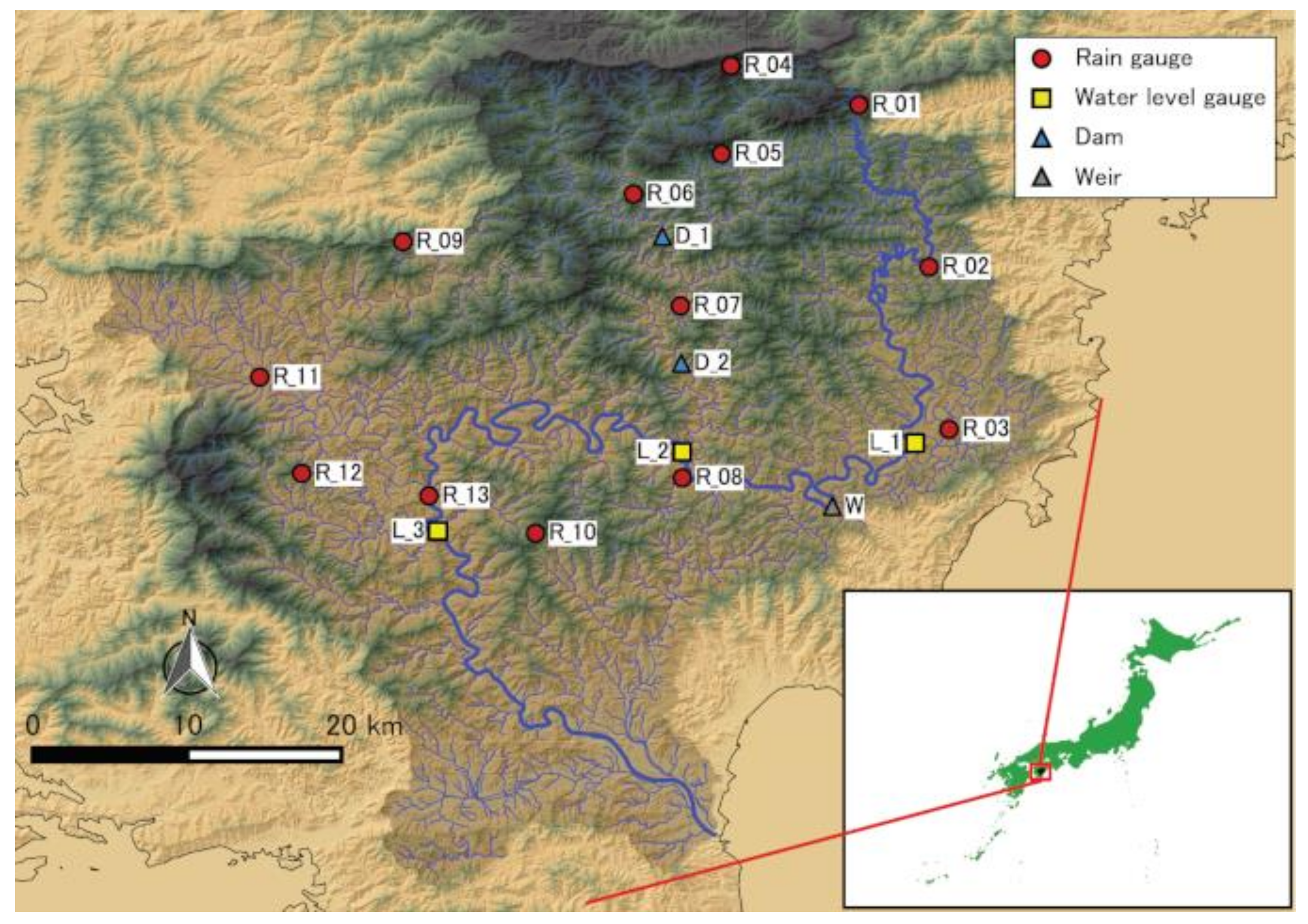
2.1. The Shimanto Watershed

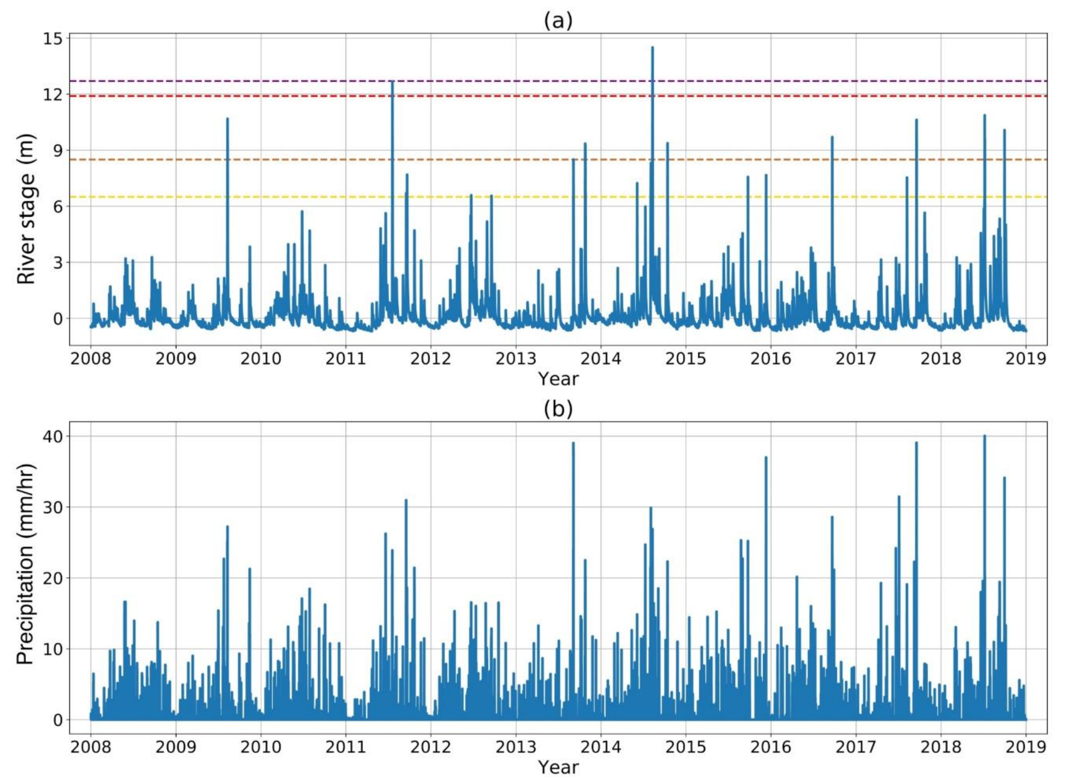
The drainage basin of this study is the Shimanto river, which is the longest river in Shikoku, the smallest of the four main Japanese islands. The official name of the river is the Watari river, but the name Shimanto is well-known to the public as “Japan’s last remaining limpid stream” [21]. The Shimanto watershed lies in the island’s southwest (Figure 1). Here, 95% of the land is forest, 4% is farmland, and 1% is residential or urban. The drainage area is 2186 km². The annual precipitation reaches about 2900 mm in the headwaters, where it is designated as a heavy rain area [22]. The source of the Shimanto has an elevation of 1336 m and the length of the main stream is 196 km, giving an average stream gradient of 0.68%. The average gradient of the upper basin ranges from 1/100 to 1/650, that of the middle basin from 1/380 to 1/1300, and that of the lower basin from 1/1200 to 1/2200. It flows into the Pacific after 319 tributaries merge. Although one of the tributaries, the Yusuhara, has two reservoirs for power generation purpose, the main stream has an 8-m weir only. The weir cannot be operated for managing the river stage, making estimation of the stage during a flood event crucial for residents.

2.2. Dataset

The target estimation/forecast was for the Tsunokawa stage observatory, which is 40 km upstream of the estuary (L_3 in Figure 1). The stage observations were from a hydrology and water-quality database [23] and arranged to an hourly dataset. The input precipitation observation data came from 13 rain gauges upstream of Tsunokawa (Figure 1) that we obtained from the hydrology and water-quality database and from the Japan Meteorological Agency (JMA, [24]). This data covers 2002 to the present with resolution of either 10 min or 1 h, but due to possible land use changes earlier in that period, we used just the hourly data for the 11 years of 2008–2018. Figure 2a shows the changes in the stage at Tsunokawa from 2008 to 2018. The stage is low during winter, then rises from summer to fall when the heavy rainfall events tend to occur, usually exceeding the level at which the flood prevention team is put on standby (yellow dashed line). During this period, the red-dashed flood-danger level was exceeded twice. The average precipitation from the 13 rain gauges (Figure 2b) shows that an hourly rainfall of 30 mm was often exceeded after 2013 and that short-term precipitation intensified.

3. Method

3.1. Modeling Concept

Water in the atmosphere precipitates in a watershed, infiltrates into the ground, moistens the soil, and then forms an interflow [25,26,27]. Some of the infiltrated water further percolates into the groundwater. Once the soil is saturated, the rain flows over the surface (overland flow) and directly flows into a channel. The interflow may emerge to the surface in a valley or saturated area, and then flow into the channel. When a pulse of rain falls to a region with a short timescale for its overland runoff, then the river stage may form a pulse-like increase [27]. However, depending on the depth of infiltration and geological characteristics, the interflow and the groundwater flow can possess various timescales that affect the river stage [25,28]. In addition, the time series of spatially distributed rainfall will influence the river stage [29]; that is, the stage is affected by soil moisture and groundwater from previous rainfall. Moreover, the river stage can respond nonlinearly to the upstream rainfall as suggested by the data in Figure 2. Therefore, the stage at a certain time t at an observatory is a complicated function of the spatial and temporal distribution of rainfall. Such a phenomenon can be inductively modeled with machine learning, in which the precipitation time series going back from time t are set as the input data, and the downstream stage as the output data (labeled data). This downstream stage is not at the estuary to avoid influences from the tide.

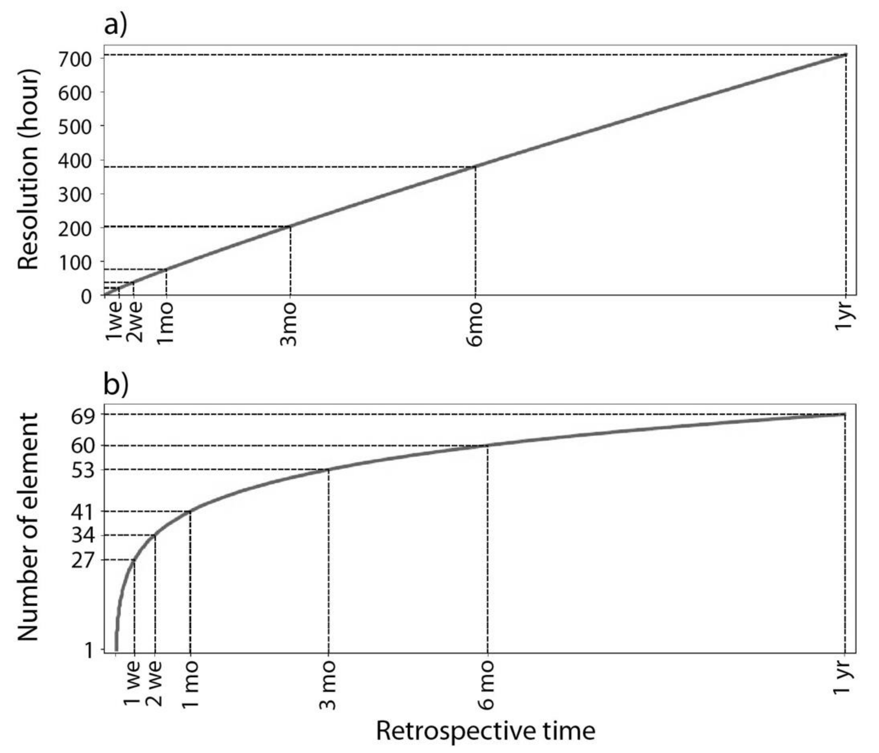
3.2. Precipitation Time Series Data as Input Data

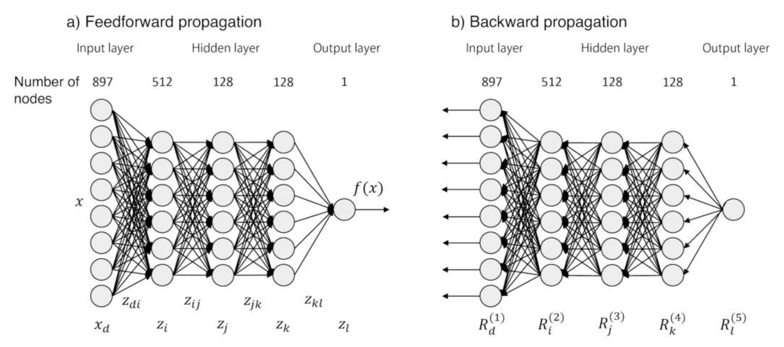
As input, we used the individual hourly time series of the 13 rain gauges upstream, not the time series averaged over these gauges, so that the model could capture the spatial relationships of rain gauges to the Tsunokawa stage, which also provided hourly stage data. Moreover, the specific slopes and geology of each branch where a rain gauge is located can presumably affect the stage.

Our preliminary investigation of the DNN modeling showed that the use of hourly rainfall time series directly as input produced a noisy time series of stage estimates. Also, after a pulse-like rainfall, the river stage would rise to a peak and then fall off with a long relaxation timescale. The hourly rainfall amount in the previous hours and days can be represented as averages over a certain time window, assuming that such past precipitation can impact the current stage through changes in the base flow. Based on these considerations, we changed to a running average method in which the number of samples to be averaged increased with the time going back from the current time. The duration of the moving, averaging y was determined for a period x hours previous to the time of evaluation to satisfy two conditions: (1) Precipitation reported within the past six hours has a one-hour resolution. (2) Precipitation one year back (365 days times 24 h) from the current time has a one-month resolution (30 days times 24 h).

$$y=\mathrm{floor}(6^{\frac{-\log 719}{\log 1460}}·x^{\frac{\log 719}{\log 1460}}+1)$$

(1)

As shown in Figure 3a, the duration of averaging (or time resolution) of rainfall that occurred 1 week back was 21 h, and that of 3 months back was 204 h. We assigned “element” numbers to these averages (Figure 3b). This averaging essentially compresses the data; for example, a 1-year time series has 8760 samples, but the manipulation reduced the sample size to 69 (Figure 3b). Thus, the method reduced the computational burden for the DNN modeling.

3.3. MLP Model

We developed a DNN model with two or more hidden layers for the regression task, using a simple multilayer perceptron (MLP). A fully-connected MLP structure consists of input, hidden, and output layers as sketched in Figure 4. It is a feedforward network in which each node weights the inputs from the previous layer and the information moves from the input to the output layer. Each connecting line has a weight, and the linear sum of node values and the weights are incremented with the biases of the layer. An activation function acts on the resulting sum to propagate the information to the next layer. The weights and biases were updated to minimize the cost function [30], a step that involves evaluating the gradients (partial derivatives). This procedure was repeated N times, where N is the number of batches multiplied by the learning epochs.

The number of nodes in the input layer of the MLP model is varied from 27 to 69 for each rain gauge, depending on the length of time gone back. The output layer has only one node. We applied the activation function PReLU [31] to each hidden layer before the output layer. As the river stage is regressed on the nodes of the last hidden layer, the mean squared error (MSE) was applied as the cost function without activation function on the output layer [32]. To avoid overfitting, a penalty term of L1 norm was added to the cost function.

We divided the above data from 2008 January to 2018 December into training, validation, and test datasets. Most of the period was used for training. The validation set was then used to examine the model structures or hyperparameters (e.g., number of hidden layers), and the test set was used to evaluate the model performance. The exact data breakdown is 2008–2014: training; 2016: validation; and 2017–2018: test. As a result, the numbers of samples for training, validation, and test sets were 61,368, 8784, and 17,520, respectively.

To optimize the structure of the MLP model, the number of hidden layers, the number of nodes, and the parameter for L1 regularization were set as hyperparameters, the combination of which were examined with the grid search method [33]. The search range is listed in

Table 1. Set of hyperparameters for the grid search method.

Hidden Layers	Nodes	L1-Regularization
2	64	0
3	128	${10}^{-8}$
4	256	${10}^{-7}$
	512	${10}^{-6}$
	1024

. Concerning the number of nodes, the structures with layers that had more nodes than the previous layer were excluded from the search (such a search operation would increase the number of input dimensions, which seems inappropriate given that the input information has to be compressed from the first layer to the last layer). The selection of hyperparameters was run for each length of the input time series to determine the best combination. In total, 480 combinations of hyperparameters were examined for each length of input time series. We set the batch size during the optimization to 100 and applied the Nesterov-accelerated Adam (Nadam) optimization method [34]. We found that for each combination of hyperparameters the errors started to converge after 25 epochs of learning, so to save on computational cost we set the number of epochs to 25. Then, the root mean squared errors (RMSEs) were calculated over the validation set by using MLP models having parameters that were obtained from 16 to 25 epochs. Among the above combinations of hyperparameters, we decided that the model with minimum average RMSE had the best structure for the length of input time series.

3.4. Model Evaluation Criteria

To examine the model performance, we used the root mean squared error (RMSE), skill score (SS), and absolute errors (AE) calculated between observed stages and model estimates. RMSE is the measure of accuracy between the observation $x_i$ and estimate $f_i$ [35]:

$$\mathrm{RMSE}=\sqrt{\frac{1}{N}{{\displaystyle \sum }}_{i=1}^N{\left(f_i-x_i\right)}^2},$$

(2)

where $N$ is the total number of samples. RMSE can be normalized by the variance of the observation to give an SS [36]:

$$\mathrm{SS}=1-\frac{{\mathrm{RMSE}}^2}{{\sigma }_x^2},$$

(3)

where ${\sigma }_x^2$ is the variance of the observation. SS is equivalent to the Nash–Sutcliffe efficiency (NSE) [37], and is a measure of the skill relative to the reference forecast being the mean of the observation, and SS = 1 means a perfect forecast. The forecast with RMSE less than the half of ${\sigma }_x$ can be considered acceptable [38,39], which corresponds to 0.75 of SS. The SS can be further decomposed into three terms:

$$\mathrm{SS}={\rho }_{fx}^2-{\left[{\rho }_{fx}-\left(\frac{{\sigma }_f}{{\sigma }_x}\right)\right]}^2-{\left[\left({\mu }_f-{\mu }_x\right)/{\sigma }_x\right]}^2.$$

(4)

The first term, ${\rho }_{fx}^2$, is the correlation coefficient squared and indicates the fraction of the total variance explained by a linear regression, and can be considered as a relative measure of potential performance among cases with various magnitude of peak stages. The second term is a measure of conditional bias or reliability (Rel), which disappears for a linear regression of a 45-degree line. The third is a measure of unconditional bias scaled by the standard deviation ${\sigma }_x$ (Bias). The mean absolute error, MAE, was calculated as:

$$\mathrm{MAE}=\frac{1}{N}{{\displaystyle \sum }}_{i=1}^N\left|f_i-x_i\right|.$$

(5)

Furthermore, the absolute error was evaluated for the time of peak level for each case.

4. Results and Discussion

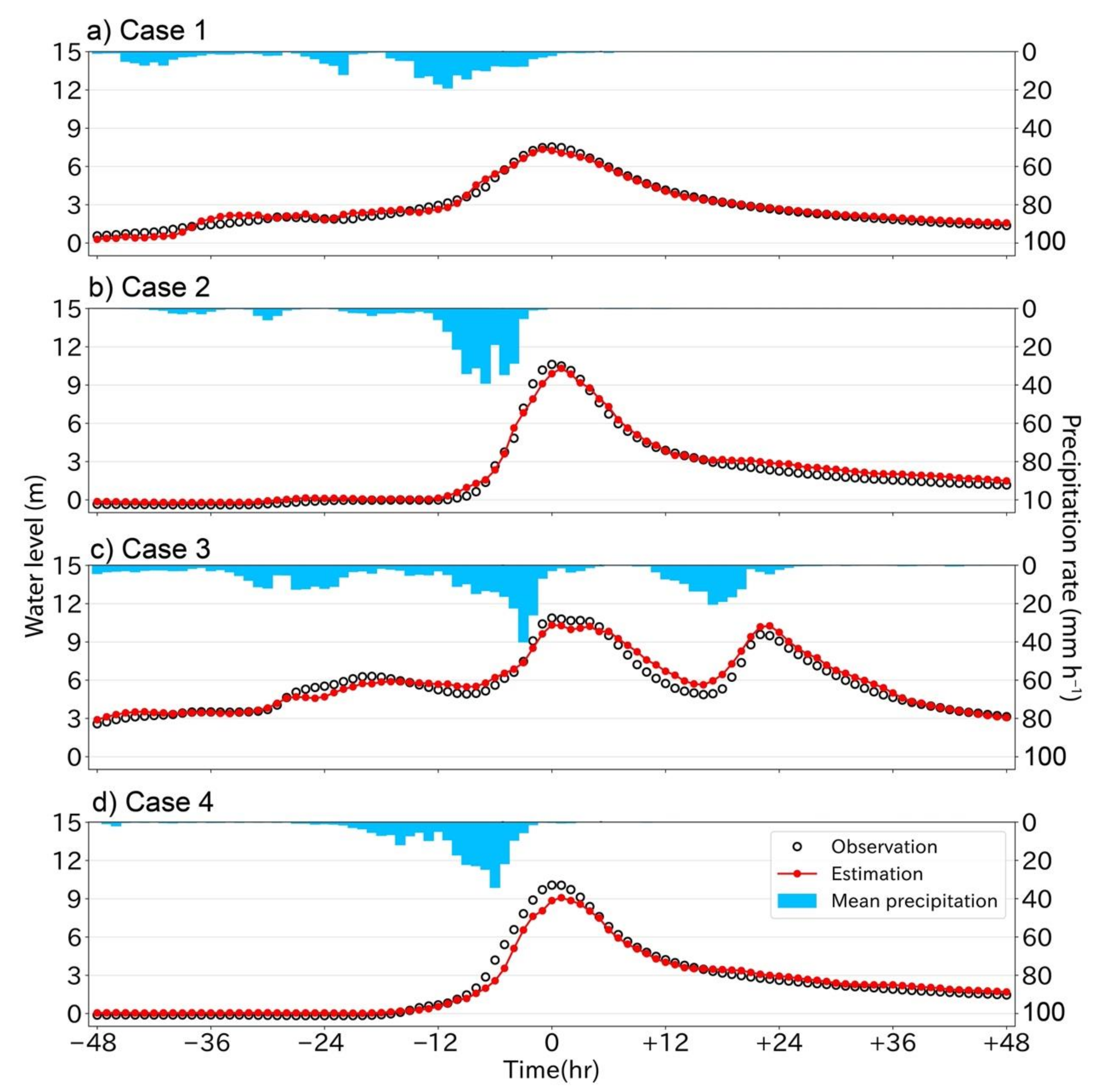
4.1. Stage Estimation

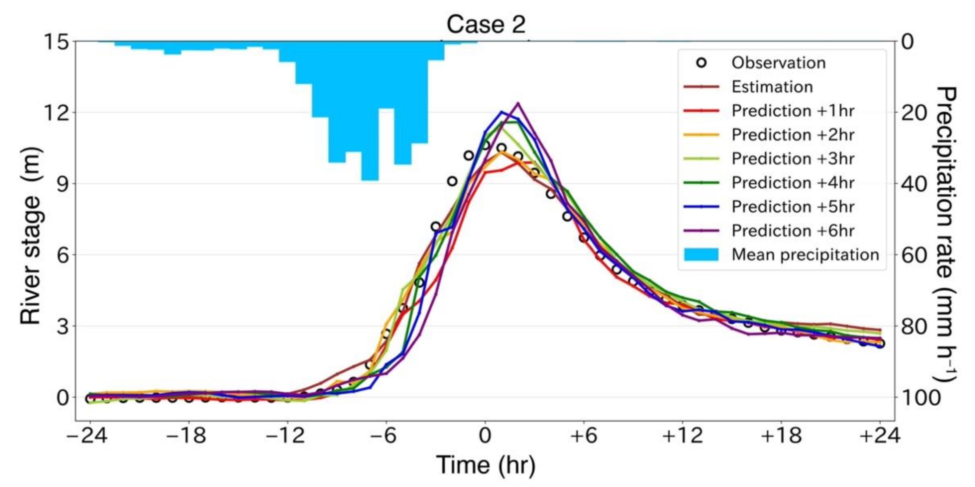
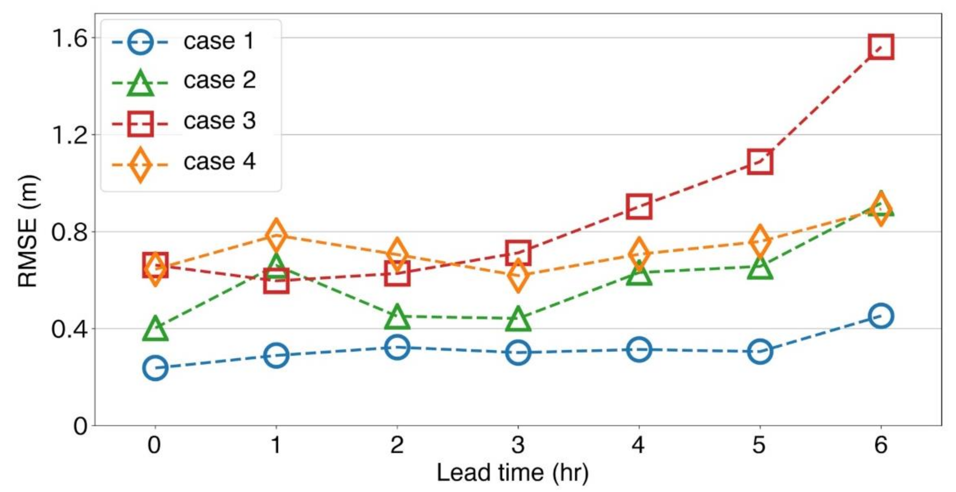
First, we examined the highest four stages in the test set. These high-stage events are as follows: case 1 on 7 August 2017, case 2 on 17 September 2017, case 3 on 7 July 2018, and case 4 on 30 September 2018. The MLP model we discuss in this section was constructed using a precipitation time series that goes back one year from the time of estimation, starting with hourly resolution. This model possesses small errors for the training set and performed qualitatively better during low-stage periods, compared with the other models with different input time lengths.

Evaluation measures were calculated within 24 h of the peak stage (

Table 2. Evaluation measures of the four flood events in the test dataset. All the measures except for AE at peak were calculated within 24 h of the peak level. The standard deviations of observed stages during the 48 h are 181, 339, 200, and 323 cm for cases 1, 2, 3, and 4, respectively.

Case	SS	${\mathit{\rho }}_{\mathit{f}\mathit{x}}^2$	Rel	Bias	AE at Peak (cm)	MAE (cm)	RMSE (cm)
	Estimation
1	0.972	0.978	0.002	0.004	50	24	30
2	0.988	0.990	0.000	0.001	55	29	37
3	0.889	0.892	0.003	0.001	69	60	67
4	0.968	0.981	0.006	0.008	89	36	57
	1-h lead time prediction
1	0.974	0.979	0.005	0.000	32	21	29
2	0.961	0.970	0.003	0.005	115	33	67
3	0.909	0.912	0.002	0.001	114	49	60
4	0.940	0.972	0.019	0.013	140	49	79
	3-h lead time prediction
1	0.972	0.983	0.005	0.006	32	24	30
2	0.983	0.986	0.002	0.001	40	33	45
3	0.870	0.879	0.003	0.006	48	57	72
4	0.963	0.983	0.013	0.007	68	42	62
	5-h lead time prediction
1	0.971	0.982	0.000	0.010	11	21	31
2	0.962	0.966	0.005	0.000	55	39	66
3	0.697	0.714	0.003	0.014	321	80	110
4	0.944	0.967	0.009	0.014	67	48	77

). The time series of estimated and observed levels are compared in Figure 5 along with hourly precipitation. Overall, the estimated stages match well with the observed stages, which is indicated by the high potential skill ${\rho }_{fx}^2$ exceeding 0.97 except for case 3. Both of the Rel and Bias values are less than 0.01, and the resulting SS values of all the cases are much higher than the acceptable criterion (>0.75). The RMSE are about 30–67 cm in the time window, relatively small compared to the peaks of about 7–11 m and ${\sigma }_x$ (see the caption of Table 2). The AEs at peak are larger than 50 cm but within 1 m. Considering the individual cases, case 1 had relatively low precipitation and river stage, which likely contributed to the small MAE. Cases 2 and 4, which had heavier rain about 12 h before their peaks, both show a delay of the rising limb, with the estimated peak time behind by about one hour, and both cases underestimated the peak levels (Figure 5). Later, as the river stages ease, they are slightly overestimated. Case 3 has three rainfall peaks exceeding 10 mm h⁻¹, with each stage peak well-captured by the model. However, the stages between the stage peaks are slightly overestimated, which resulted in the lowest potential skill, and therefore the lowest SS.

In cases where a precipitation time series similar to the test dataset is not available in the training and validation sets, the estimation errors can be large. Even though case 2 shows a similar change of stage over time to case 4, the latter had a larger underestimate and a much larger AE at peak (=89 cm) (Table 2). This is not desirable given that the evacuation judgment stage is 11.9 m (Figure 2). According to the time series in Figure 6, case 2 had little rainfall within one month of the stage peak, whereas case 4 had several notable rainfall events within the month preceding the flood. The difference in the precipitation pattern during that preceding period probably led to a difference in soil moisture in the watershed, and hence to the retarded accuracy of case 4. With regard to the soil moisture and precipitation occurrences, a condition such as case 2 was probably better learned from the training and validation sets, but a condition such as case 4, in which soil moisture increased with time, was probably not learned as well. Physically, the model simulated a situation where the rainfall over-infiltrated into the soil, leading to an underestimate of the overland flow and thus underestimation of the peak.

When there are not enough samples of heavy rainfall events in the training and validation sets that are spatially similar to those in the test set, the estimation errors can be potentially large. To compare the characteristics of precipitation in the training and test sets, we investigated the fraction of total precipitation at each rain gauge for each flood event. For the statistics, we used the top 12 flood events from 2008–2014 in the training set, and the four events for the above test set. As defined below, the precipitation accumulation p_iⁿ for flood event $n$ and for rain gauge i was calculated by the 24-h window centered on the stage peak:

$$p_i^n={\displaystyle \sum }_{t=t_p^n-12}^{t_p^n+12}{r}_{i,t}^n$$

(6)

where $t_p^n$ is the peak time of the stage. Summing over all 13 gauges, the total accumulation $p^n$ is:

$$p^n={{\displaystyle \sum }}_{i=1}^{13}{p}_i^n$$

(7)

Thus, the fraction for the gauge $i$ is:

$$P_i^n=\frac{p_i^n}{p^n}.$$

(8)

Figure 7 shows the fraction of the 24-h accumulation centered on the time of stage peak $P_i^n$. A larger fraction may indicate a larger contribution to the flood (the area coverage of each gauge is not considered for simplicity). The rain gauges are arranged from the most upstream at left (R_01) to the most downstream at right (R_13). The generally decreasing trend shows that the precipitation at the upstream gauges at higher altitudes contributed more than those further downstream. Cases 1, 2, and 4 show a pattern similar to the training set, and they are within the 25 to 75 percentiles except for R_01. However, case 3 indicates a quite different pattern compared with the training set, with the fraction at the upstream gauges relatively small and those downstream relatively large. Furthermore, several gauges have values outside the 25th and 75th percentiles. This difference in the spatial distribution of accumulation is most likely the reason why the ${\rho }_{fx}^2$ and RMSE of case 3 are the worst.

4.2. Stage Forecast

Here we examine an MLP model that learns the relationships between the one-year precipitation time series up to the present and the river stage at t h later. In other words, this is the model that forecasts the stage at t h from the current time. Note that the MLP models were constructed for each lead time t (t = 1, 2, …, 6 h). The same precipitation time series and hyperparameters were used to construct the MLP models as used for that in the previous section.

The time series of the forecast stage with lead times t of 1, 2, …, 6 h are shown for case 2 in Figure 8. The evaluation measures are listed for lead times of 1, 3, and 5 h in Table 2. Forecasts with 1 and 2 h lead times show high ${\rho }_{fx}^2$ (>0.97). However, due to delays of the level peaks, AE at peak reaches about 110 and 92 cm, respectively. The 3-h forecast predicts a larger peak than the observation, as do those for the 4–6-h forecasts. As a result, the AEs at peak were improved compared to 1 and 2 h lead times. A closer look at the 4-h forecast indicates that the stage is about half of that observed at −6 h, and the predicted flood peak is late. The same issues also occur for the 5- and 6-h forecasts. The errors are probably caused by a lack of precipitation information during t h. The accurate prediction from the 3-h forecast suggests that the precipitation producing the stage peak arrived via surface runoff at Tsunokawa after about three hours.

Figure 9 shows the dependence of the RMSE on the lead time for all four cases. For cases 2–4 with the large magnitude of stage peak the RMSEs are similar among the forecasts when the lead time is three hours or less. However, case 3 shows a rapid increase of the RMSE after a 2-h lead time. This case has a larger fraction of precipitation downstream (Figure 7). This suggests that when stage forecasts are made without the use of precipitation forecasts, especially cases with large fraction of precipitation occurring in the downstream, the errors can dramatically increase with the lead time.

Considering the MLP framework above, a MLP model for a t-hour stage forecast may be developed with a combined time series of observed and forecast precipitation to learn the stage observed at t hours. In this section, we discussed the case where the forecast precipitation data is not available up to the time when the stage forecast is made. Given that JMA produces precipitation forecasts up to 15 h ahead, then by using their time series, a stage forecasting may be produced with a 15-h lead time by using the current MLP framework for estimation. In such a case, any decrease in the accuracy of the precipitation forecast would likely decrease the accuracy of the river-stage forecast.

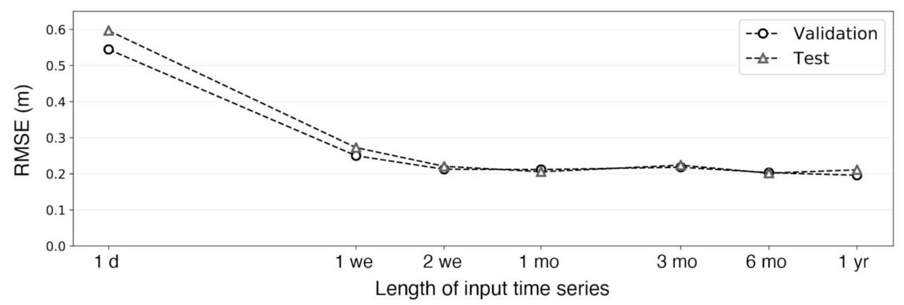
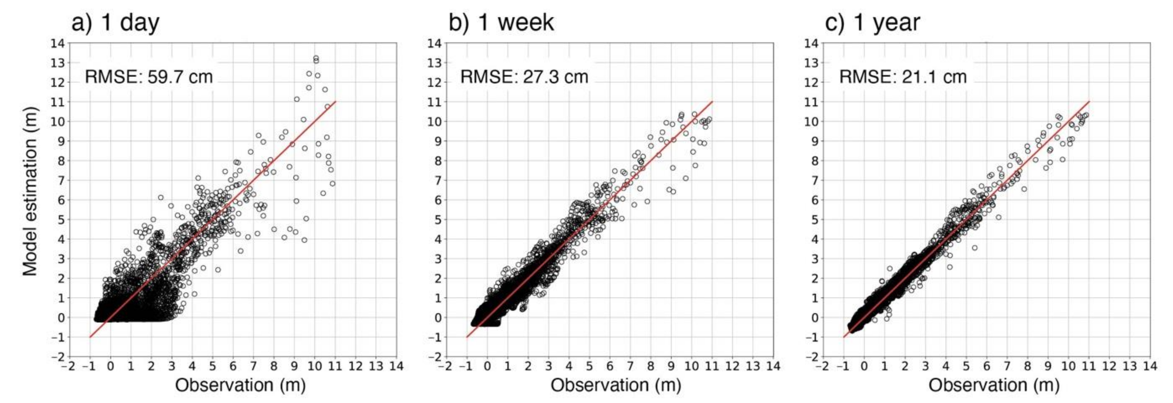
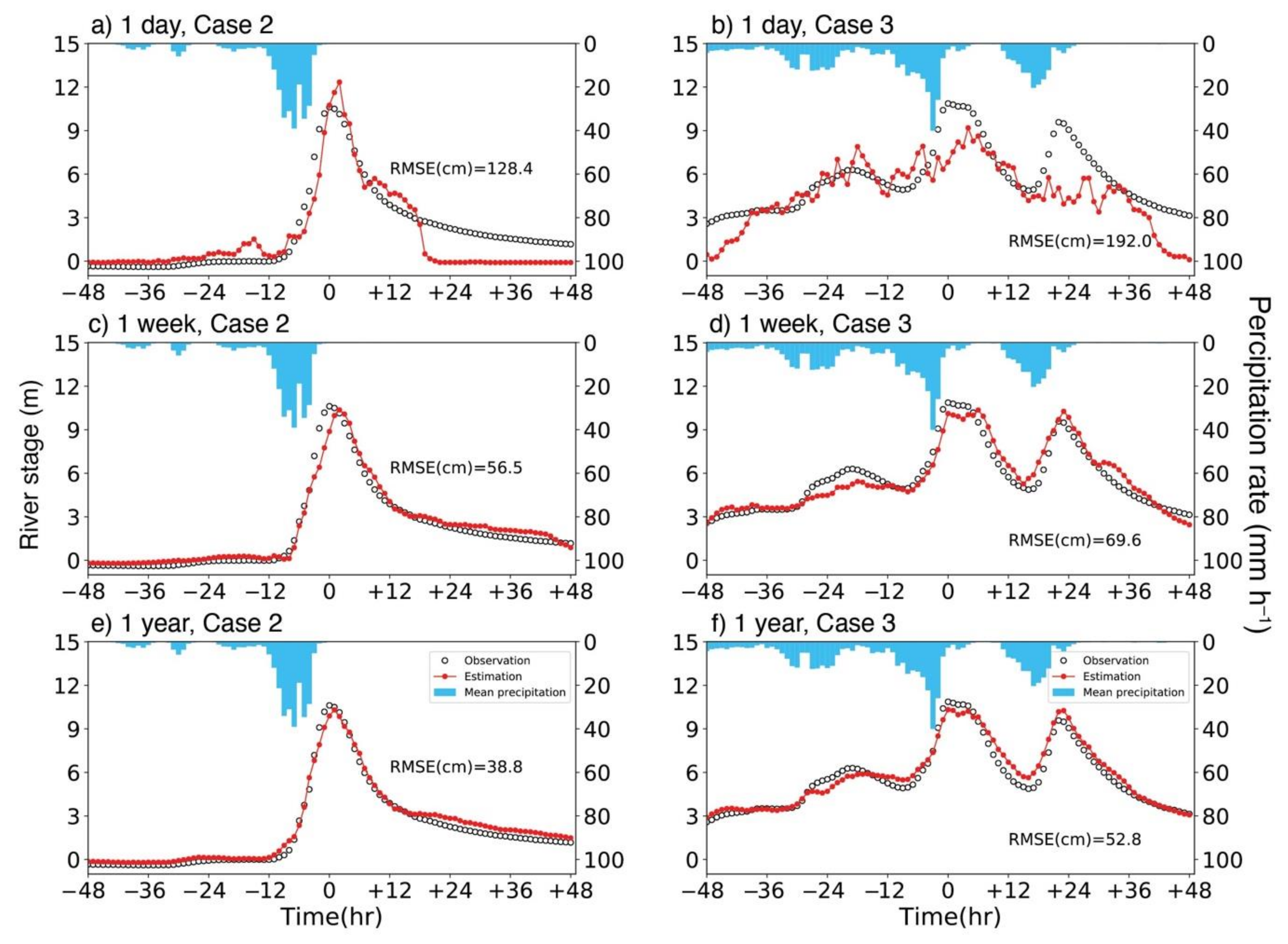
4.3. Effects of Precipitation Time Series Length on Stage Estimation

In above sections we discussed the stage estimation and forecast based on MLP models that use a one-year precipitation time series as the input dataset. Here, we examine how changing the precipitation time series length affects the stage estimation. This length was set to one day, one week, two weeks, one month, three months, six months, and one year. For a given length, an MLP model was developed and its hyperparameters were optimized.

Figure 10 shows the RMSEs between the estimated stage and observation for the seven MLP models for both the validation and the test datasets. For both datasets, the RMSEs dramatically decrease from one day to one week, reaching about 0.2 m after one month. Note that Nakane et al. [20] found that the RMSE continued to decrease monotonically to 0.156 m after 720 days they used a method involving similar MLP models, but shorter time-averaging.) Therefore, we cannot assert that the information of precipitation that was observed more than one-month ago is not necessary.

The improvement in modeling fit for longer precipitation time series can also be seen in the scatterplots (Figure 11). For the one-year precipitation time series, the points are distributed close to the 1:1 line (red, in Figure 11c). The one-week case is similar, but with more spread, corresponding to the larger RMSE than the one-year case (Figure 11b). The case with a one-day time series shows a large number of points are located below the red line over the range of observation of 3 m, indicating that the model tends to underestimate the stage. The reason behind the large one-day RMSE compared to one week is examined next.

Consider the relation of stage estimate to precipitation pattern for the one-day, one-week, and one-year MLP models for flood cases 2 and 3 in Figure 12. The importance of the length of input time series is evident in the one-day series for case 2 (Figure 12a) when the stage estimate suddenly dropped just after 12 h and then stayed near 0 m. At 24 h, the average precipitation during the past 24 h was 0, which explains the estimate being about 0 m. Case 3 (Figure 12, right column) had intermittent heavy rainfall observed in the upstream. The one-day MLP model poorly estimated the second stage peak and essentially missed the third peak (Figure 12b). This model’s estimate is remarkably noisy presumably due to the absence of precipitation information before 24-h back. When the length of input time series increased to one week, the three peaks in case 3 were reproduced nicely (Figure 12d), but the match between the estimates and observations was even better with the one-year input time series (Figure 12f). From these results, we concluded that during flooding events the role of soil moisture and ground water is extremely important one day to one week before a rainfall event, and the runoff process with larger timescales associated with precipitation that occurred one week to one year in the past also cannot be ignored.

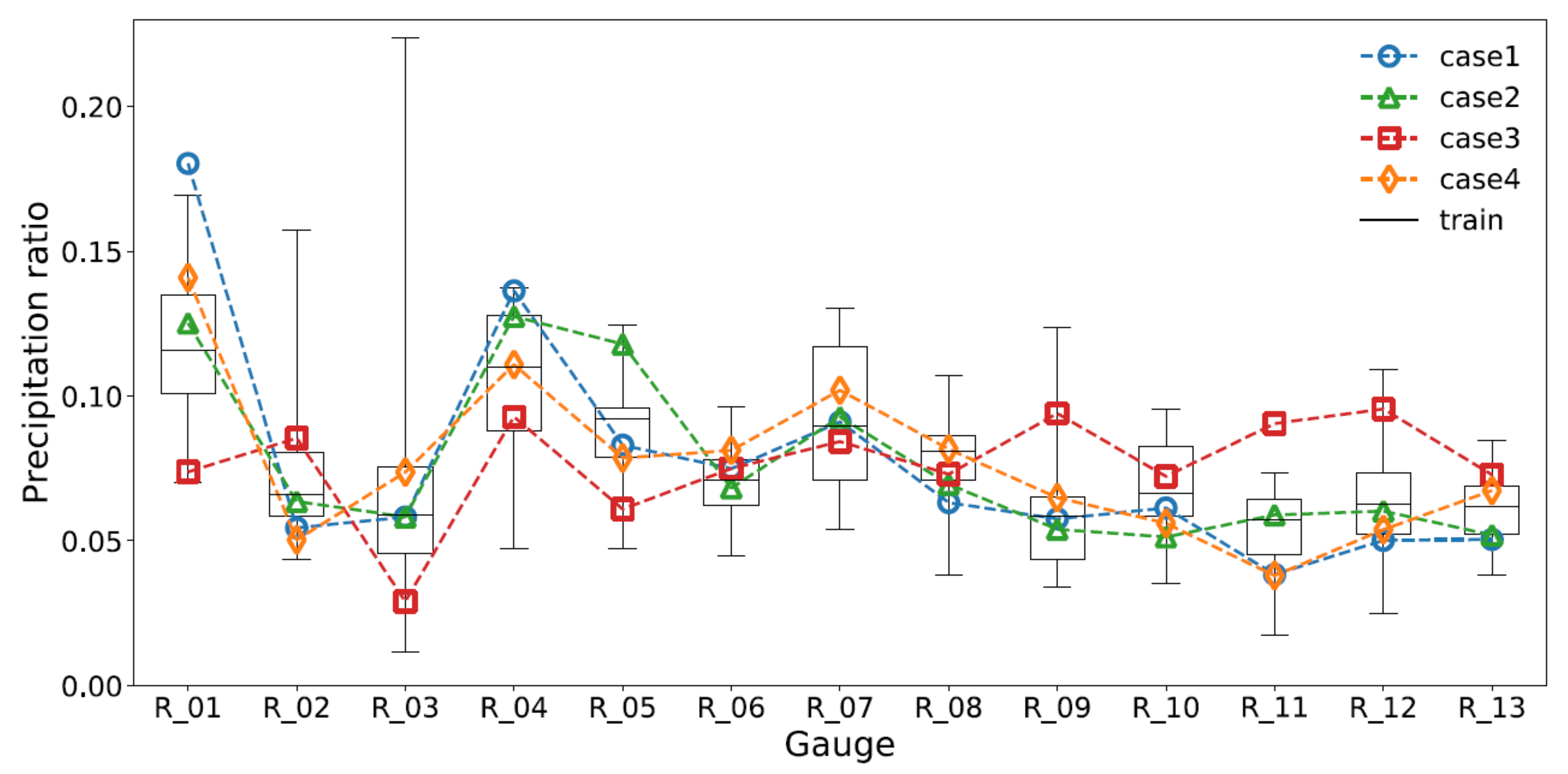
4.4. Stage Estimation Sensitivity to the Rain Gauges

How does a given rain gauge and rainfall event affect the flood stage? The typical way to measure an output’s sensitivity to an input is by perturbing the input and noting the change in output. However, in this case there are hundreds of input variables for the single output variable (the stage). Thus, we used layer-wise relevance propagation (LRP) [40], a visualization technique, to determine the relationship between stage and precipitation time series. The relationship enables us to examine the time of precipitation arrival to the stage, as well as the sensitivity of the stage, to a given precipitation event from a given rain gauge.

LRP measures the overall contribution of each input variable by propagating the contribution through the learned neural network for a specific instance of output. Rises in the river stage are, in general, formed not by the independent precipitation event at a certain moment in the past, but by a distribution of precipitation over a period of time. Therefore, for the MLP models here, it is more appropriate to measure the overall relevance of the past precipitation time series than to calculate the stage’s sensitivity to the precipitation at a certain moment. Also, LRP can be run for estimates and forecasts for real flood events, providing an explanation of the model behavior for a given flood event. Therefore, it is an appropriate method to characterize the MLP models.

LRP quantifies the contribution of a given precipitation input to the model output, calling it the “relevance” of that input. A higher numerical value for the relevance indicates a higher contribution. Details on its calculation are in the Appendix A; here, we focus on the results.

The relevance of the precipitation inputs for the stage estimate at a certain time was calculated for case 2 over 24 h of the flood event. In Figure 13, the relevance of precipitation inputs for the stage at a certain time, shown as the black contours, can be examined by specifying the time on the abscissa and examining the contours from top down, which corresponds to the retrospective time. The top panel has results for the gauge furthest upstream, the bottom panel being for the gauge closest to Tsunokawa, L3 (see Figure 1). For the precipitation inputs, we analyze just the first 14 (of the total 69).

Figure 13. Relevance map of the stage estimation MLP model for case 2 and three rain gauges along the main stream (Figure 1). The abscissa is the time from the stage peak. The left ordinate is the precipitation element (

Table 3. Time elements prior to current time t and their time resolutions.

Element	Time (h)	Resolution (h)
E_01	t	1
E_02	t − 1	1
E_03	t − 2	1
E_04	t − 3	1
E_05	t − 4	1
E_06	t − 5	1
E_07	t − 6~t − 7	2
E_08	t − 8~t − 9	2
E_09	t − 10~t − 11	2
E_10	t − 12~t − 13	2
E_11	t − 14~t − 16	3
E_12	t − 17~t − 19	3
E_13	t − 20~t − 22	3
E_14	t − 23~t − 26	4

), with its relevance marked as black contours. The right ordinate is the stage, with the white dashed curves showing observed (white-filled circles) and estimated (red-filled circles) stages. Color fill is input precipitation. (a) Gauge R_01. (b) Gauge R_08. (c) Gauge R_13. The red arrows indicate the estimation of the arrival time of precipitation.

Figure 13. Relevance map of the stage estimation MLP model for case 2 and three rain gauges along the main stream (Figure 1). The abscissa is the time from the stage peak. The left ordinate is the precipitation element (Table 3), with its relevance marked as black contours. The right ordinate is the stage, with the white dashed curves showing observed (white-filled circles) and estimated (red-filled circles) stages. Color fill is input precipitation. (a) Gauge R_01. (b) Gauge R_08. (c) Gauge R_13. The red arrows indicate the estimation of the arrival time of precipitation.

In general, precipitation at a certain time shifts toward a larger element number as the estimation time progresses, and the time resolution gets worse, combining more precipitation events as the time goes back from the estimation time. For instance, in Figure 13a, the precipitation (color fill) of E_01 at −9 h is the same as that of E_02 at −8 h, and at −3 h the precipitation is contained in the E_07 element through the two-hour average. The sequence of precipitation that started at −10 h lasted up to −4 h, and the number of elements in the sequence gradually decreases along the vertical axis toward +12 h so as to remain as the input information.

Consider first the relevance for R_01 (Figure 13a). The sequence of precipitation events that started at −10 h show a rise in relevance (black contours) at −4 h and at E_07. At −4 h the most contributed precipitation to the stage estimate (about 5 m) is the one observed at −10 h, the time when the stage started to rise. For 0–4 h the relevance shows a peak at E_08, indicating that the precipitation that fell 8 or 9 h prior contributed to the stage up to four h after the peak. Then, from 4 to 6 h the maximum relevance values occur at E_08 and E_09, as marked with the red arrows. Based on this pattern, the time for precipitation that fell at R_01 to reach the Tsunokawa stage observatory is about 8–11 h. Furthermore, there are large values of relevance associated with the sequence of precipitation events up to 7 h, and precipitation peaks follow the relevance peaks closely. Moreover, as the relevance value is particularly large after the stage peak, this rain gauge has the geographical characteristic of being a significant contributor when the stage decreased rather than when it increased.

Now consider the relevance for gauge R_08 (Figure 13b). The relevance starts to increase at −4 h and at E_06, reaching a maximum value at 1 h and E_08. This pattern indicates an arrival time of precipitation of about 8–9 h. In contrast with R_01 further upstream, this gauge makes its maximum contribution at the time of the stage peak. Thus, for the same arrival time of precipitation, the gauge further downstream has a different timing of its largest contribution. In addition, it has a narrower spread of relevance along the estimation time, suggesting that the precipitation that contributes to the flood peak occurred over a shorter time period.

Finally, consider R_13, the gauge furthest downstream and closest to the stage. Its relevance starts to increase at −6 h and E_02, reaching a maximum at either −5 h and E_03 or at 0 h and E_07. This pattern indicates an arrival time of precipitation of about 2–7 h. The relevance is larger before the peak, so for this gauge the precipitation contributed most from the rising limb to the peak.

Let d_{R_n} be the distance between the Tsunokawa station and R_n. Figure 1 indicates that d_{R_13} < d_{R_08} < d_{R_01}. The relevance analyzed above suggests the arrival time of precipitation t_{R_n} follows t_{R_13} (2–7) < t_{R_08} (8–9) $\le$ t_{R_01} (8–11). The t_{R_13} and t_{R_08} are clearly different, and at most about 6–7 h traveling time in between. This suggests that the MLP model represents the geographical distance in the arrival time of precipitation. On the other hand, the nearly equal timescales between gauges 1 and 8 are unclear. Gauge R_01 experienced about twice the precipitation than that at R_08 during case 2 and lies in a steeper, higher region than R_08 (Figure 1). The steeper slope could reduce the arrival time of R_01, but other factors such as vegetation, soil types, and local topography may also influence the relevance. Future research is required to clarify the physical implication of the relevance in detail.

4.5. Comparison with a Previous Research

In this section the method proposed in this research is compared against a MLP model of Hitokoto et al. [16]. The main difference lies in the type and number of input data. The Hitokoto’s model, hereafter H_t model (t being the lead time), uses (1) river stages at a target location (L_3 of Figure A1), (2) temporal changes in stages at upstream locations, and (3) rainfall forecasts in the upstream (

Table 4. The input and output variables for the Hitokoto’s MLP model. The time of each piece of data is shown relative to the current time, and the lead time t given in hours.

	Input		Output
Type	Number of gauges	Time	Change in the river stage measured at the Tsunokawa observatory between 0 and t hour.
River stage	1	−1, 0
Hourly change in stage	3	−2, −1, 0
Hourly rainfall	13	t − 5 to t − 1

). In order to construct the model for the Shimanto river basin, temporal changes in stages were calculated at the three locations (L_1, L_2, and L_3). As in [16], the observed rainfall at 13 gauges was used as a “perfect” forecast. Note that the rainfall data is required from t − 5 to t − 1 h in the future for the forecast with t hour lead time.

Since the observed rainfall was used as forecast up to one hour before the forecast in the H_t model, we can compare it against the proposed model with one-hour lead time discussed in Section 4.2. It is called the P_L model. Furthermore, as H_t model predicts stage changes, we constructed another MLP model, P_CL_t that predicts changes in stage instead of the stages themselves and uses rainfall data from up to one hour before the forecast. For instance, 6-h lead time forecasts of H_6 and P_CL_6 both require one- to five-hour rainfall forecasts to make a water change between current and 6 h later. P_CL_6 basically replaces the stage observations required for H_6 with year-long rainfall time series observations.

The evaluation measures for H_t and P_CL_t are listed in

Table 5. Same as Table 2 except for this is for H_t and P_CL_t. The lead time is defined with respect to the latest time of stage observation at Tsunokawa.

Case	SS	${\mathit{\rho }}_{\mathit{f}\mathit{x}}^2$	Rel	Bias	AE at Peak [cm]	MAE [cm]	RMSE [cm]
	H_1 1-h lead time prediction
1	0.999	0.999	0.000	0.000	0	4	7
2	0.991	0.992	0.000	0.001	10	13	33
3	0.982	0.983	0.000	0.001	14	15	26
4	0.998	0.998	0.000	0.000	5	8	16
	PCL_1 1-h lead time prediction
1	0.997	0.998	0.000	0.000	11	6	9
2	0.994	0.995	0.000	0.000	1	12	25
3	0.990	0.991	0.000	0.000	20	15	20
4	0.998	0.998	0.000	0.000	6	8	14
	H_2 2-h lead time prediction
1	0.996	0.997	0.001	0.000	7	7	11
2	0.970	0.974	0.001	0.003	50	25	59
3	0.929	0.932	0.000	0.003	100	32	53
4	0.991	0.992	0.001	0.001	15	16	31
	PCL_2 2-h lead time prediction
1	0.978	0.982	0.004	0.000	52	20	27
2	0.974	0.977	0.002	0.000	85	25	54
3	0.926	0.935	0.008	0.001	139	36	54
4	0.992	0.994	0.003	0.000	80	19	29
	H_3 3-h lead time prediction
1	0.992	0.994	0.001	0.000	19	11	16
2	0.945	0.953	0.003	0.005	152	37	80
3	0.862	0.870	0.001	0.007	194	48	74
4	0.982	0.985	0.002	0.001	68	21	44
	PCL_3 3-h lead time prediction
1	0.950	0.960	0.010	0.000	94	30	40
2	0.942	0.947	0.005	0.000	230	41	82
3	0.819	0.840	0.021	0.000	240	60	85
4	0.974	0.981	0.007	0.000	149	33	52

. The one-hour lead time predictions by these models show very high SSs (>0.98) for the four flood cases, and the RMSEs are about one third of the P_L model (see 1-h lead time prediction in Table 2). The AEs at peak are less than 20 cm, and better than the P_L model. Those for two-hour lead time predictions still maintain higher SSs and slightly lower AEs at peak than the P_L model. Therefore, use of stage changes as a label of MLPs instead of the level itself may lead to more accurate forecasts with one- and two-hour lead times. Since H_t and P_CL_t show similar high evaluation measures for these short lead times, it is possible to replace river stage and stage changes with rainfall time series in the input.

Actually, H_t predictions show increases in RMSEs and MAEs with lead time although the information on stages is included in the model. This is probably because the relationship between the stage changes in the future and those in the past become unclear with the lead time. P_CL_t also shows monotonic increases in RMSEs with lead time, which is larger than H_t and indicates that the rainfall in the past has weaker association with the stage changes in the future than with the stage changes in the past.

It turned out that P_L outperforms H_t and P_CL_t for lead times of three (Table 5) and four to six hours (not shown). This indicates that the direct prediction of stages is better used as the label of MLPs than that of stage changes in the case of using long-term rainfall time series as input and for the longer lead times. As described in Section 3.1, the rainfall in the past and the stage downstream are correlated to some extent. On the other hand, the stage changes are more associated with the changes in the storage as further improvement was evidently achieved by introducing the storage information to the input [41]. Therefore, when precipitation forecast products with high accuracy are available, use of stages as a label, i.e., the P_L model, is more desirable than use of of stage changes. Another interesting point is that the proposed models with even three- and five-hour lead time predictions can produce smaller AEs at peak and RMSEs for some cases than H_t and P_CL_t (see Table 2), even though the rainfall information is absent three or five hours before the forecast stage. Thus, it is worthy of constructing the simple proposed MLP models even if the latest rainfall data is not available.

5. Conclusions

In this study, we developed multilayer perceptron (MLP) models to estimate and forecast a river stage in the Shimanto river watershed. This watershed lies in a mild, rain-heavy mountain region covered with forests. The models were developed solely based on the observed long-term precipitation and stage time series, and then tested. The main findings are:

• Models that estimated the stage at the latest time of the input precipitation time series captured the time fluctuation of stages with RMSEs between 30 and 67 cm for flood peaks of about 10 m.
• Stage forecasts were made 1 to 6 h after the latest precipitation observation with the MLP framework. The performance was highly accurate with up to a 3 h lead time. This suggests that the current precipitation information in the watershed contributes significantly to the stage 3 h later.
• Input of precipitation that occurred one day to one week prior to a flood influences the river stage estimate during flood events, which is likely related to the infiltration to soils and interflow processes. Precipitation further back, up to one year, has non-negligible impacts on the base flow, which implies that the MLP models learned the ground water flow over long timescales.
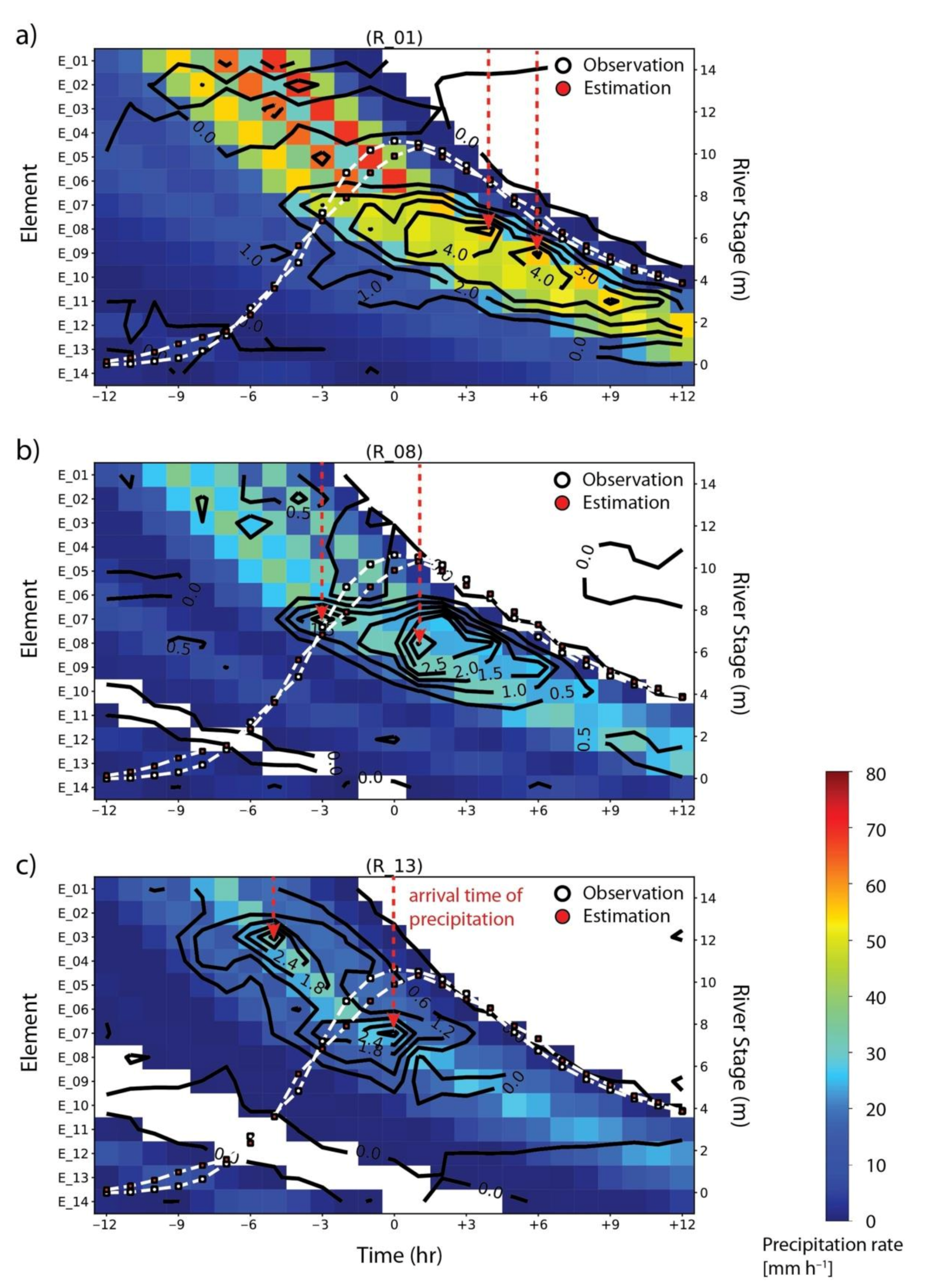
• Use of LRP (layer-wise relevance propagation) enabled us to estimate the arrival time of precipitation based on the increase of the contribution (called relevance). The arrival time correlated to the distance between rain gauge and stage observatory, indicating that the MLP models likely captured the geographical characteristics of the watershed. However, more detailed analysis is required to relate the arrival time to physical parameters such as gradients and vegetation.
• Comparison with a previous MLP modeling and the proposed modeling indicates that use of stage changes as a label gives more accurate prediction for one- to two-hour forecasts than the use of stages themselves, and rainfall time series can substitute the stage changes observed upstream in the input. Furthermore, the proposed models with the lead time of three and five hours performed better than the previous models in some cases.

The inductive (or empirical) modeling proposed in this study does not include relevant physical processes explicitly. Even so, the models exhibited reasonable physical behavior. Visualization techniques such as LRP help users to interpret the model characteristics, and it can enhance the reliability of the MLP models as a practical hazard-prevention tool. However, due to the inductive nature of the method, accurate predictions require that the model developers carefully select training sets that are expected to be similar to any anticipated flood events.

The advantage of the MLP modeling is in allowing one to construct models for forest-covered watersheds with complicated topography only from long-term time series of precipitation and stage. In contrast, physical-based modeling typically requires information on topography, gradient, vegetation, and soil type that can be cumbersome to acquire. Also, the MLP modeling does not require involved parameter tuning, which can save on manpower and cost. Furthermore, if accurate precipitation forecast datasets are available as the input, a stage forecast MLP model can be constructed. Future research is warranted to examine the ability of the MLP model to remove biases in the precipitation forecast and to effectively use the precipitation forecasts.

References

1. Intergovernmental Panel on Climate Change (IPCC). Climate Change 2013, The Physical Science Basis. Available online: https://archive.ipcc.ch/report/ar5/wg1/ (accessed on 12 December 2021).
2. Japan Meteorological Agency (JMA). Special Feature: To Protect Lives and Livelihoods from the Intensifying Torrential Rain Disaster. Available online: https://www.jma.go.jp/jma/kishou/books/hakusho/2020/index1.html (accessed on 12 December 2021).
3. Kawase, H.; Yamaguchi, M.; Imada, Y.; Hayashi, S.; Murata, A.; Nakaegawa, T.; Miyasaka, T.; Takayabu, I. Enhancement of extremely heavy precipitation induced by Typhoon Hagibis (2019) due to historical warming. SOLA 2021, 17, 7–13. [Google Scholar] [CrossRef]
4. Kato, R.; Shimose, K.; Shimizu, S. Predictability of precipitation caused by linear precipitation systems during the July 2017 Northern Kyushu heavy rain event using a cloud-resolving numerical weather prediction model. J. Disaster Res. 2018, 13, 846–859. [Google Scholar] [CrossRef]
5. Uchida, T.; Akamatsu, Y.; Suzuki, Y.; Moriguchi, S.; Oikawa, Y.; Shirahata, H.; Izumi, N. Special issue on the heavy rain event of July 2018 in western Japan. J. JSCE 2021, 9, 1–7. [Google Scholar] [CrossRef]
6. Ministry of the Environment; Government of Japan. Natural Environment of Japan. Available online: https://www.env.go.jp/en/nature/npr/ncj/section1.html (accessed on 12 December 2021).
7. Kadoya, M.; Fukushima, A. Concentration time of flood in small or medium river basin. Disaster Prev. Res. Inst. Annu. 1976, 19, 143–152. [Google Scholar]
8. Kanda, T.; Kanki, K.; Yoshioka, Y. Estimation of time of concentration for overland flow on a sloping plane. J. JSCE 1990, 417, 53–62. [Google Scholar] [CrossRef] [Green Version]
9. Kubo, T.; Yamaji, H.; Okabayashi, F.; Shinkawa, K.; Kakehi, Y. Report of the Monobe river flood in July 2018. J. JSCE 2019, 75, 208–213. [Google Scholar] [CrossRef]
10. Kikumori, Y.; Ikeuchi, K.; Egashira, S.; Ito, H. Development of flood early warning methodologies using rational formula model in mountainous rivers. J. JSCE 2018, 74, I_1345–I_1350. [Google Scholar] [CrossRef]
11. Shen, C. A Transdisciplinary Review of Deep Learning Research and Its Relevance for Water Resources Scientists. Water Resour. Res. 2018, 561, 918–929. [Google Scholar] [CrossRef]
12. Gude, V.; Corns, S.; Long, S. Flood prediction and uncertainty estimation using deep learning. Water 2020, 12, 884. [Google Scholar] [CrossRef] [Green Version]
13. Rao, G.S.; Giridhar, M.V.S.S. Daily Runoff Forecasting using Artificial Neural Network. Int. J. Sci. Eng. Res. 2016, 7, 478–484. [Google Scholar]
14. Chanu, S.N.; Kumar, P. Modelling of Daily Rainfall-Runoff Using Multi-Layer Perceptron Based Artificial Neural Network and Multi-Linear Regression Techniques in A Himalayan Watershed. Indian J. Hill Farming 2018, 31, 166–176. [Google Scholar]
15. Oluwatobi, A.; Gbenga, O.; Joy, A.; Oluwole, A. Modeling and simulation of river discharge using artificial neural networks. J. Sci. 2018, 20, 362–370. [Google Scholar] [CrossRef]
16. Hitokoto, M.; Sakuraba, M.; Sei, Y. Development of the real-time river stage prediction method using deep learning. J. JSCE 2017, 5, 422–429. [Google Scholar] [CrossRef] [Green Version]
17. Nakano, H. Forest Hydrology; Kyoritsu Publisher: Tokyo, Japan, 1976; p. 228. [Google Scholar]
18. Hashino, M.; Yao, H.; Yoshida, H. Studies and evaluations on interception processes during rainfall based on a tank model. J. Hydrol. 2002, 255, 1–11. [Google Scholar] [CrossRef]
19. Nakane, H.; Wakatsuki, Y. Startup of Deep Learning Application to Environmental Research. Kochi Univ. Technol. Res. Bull. 2018, 15, 111–120. [Google Scholar]
20. Nakane, H.; Wakatsuki, Y.; Yamamoto, K.; Takeda, T.; Hashino, T. Application of Deep Learning to River Disaster Prevention and Environmental Conservation—On the Shimanto River and Kagami River Water Levels, and the Ohdo Dam Inflow of the Niyodo River. Kochi Univ. Technol. Res. Bull. 2019, 16, 227–244. [Google Scholar]
21. Organization for Promotion of Tourism in SHIKOKU, Shimanto River. Available online: https://shikoku-tourism.com/en/see-and-do/10071 (accessed on 12 December 2021).
22. Ministry of Land, Infrastructure, Transport and Tourism (MLIT). River Maintenance Plan, Overview of Watari-Gawa Basin. Available online: http://www.skr.mlit.go.jp/nakamura/seibikeikaku/about/outline.html (accessed on 12 December 2021).
23. Ministry of Land, Infrastructure, Transport and Tourism. Water Information System. Available online: http://www1.river.go.jp/ (accessed on 12 December 2021).
24. Japan Meteorological Agency. Available online: http://www.jma.go.jp/jma/indexe.html (accessed on 12 December 2021).
25. Maidment, D.R. Chapter 9 Flood Runoff. In Handbook of Hydrology; McGaw-Hill: New York, NY, USA, 1992. [Google Scholar]
26. Takasao, T. Occurrence area of direct runoff and its variation process. Disaster Prev. Res. Inst. Annu. 1963, 6, 166–180. [Google Scholar]
27. Tanaka, T.; Yasuhara, M.; Sakai, H. The Hachioji Experimental Basin Study—Storm Runoff Processes and the Mechanism of its Generation. J. Hydrol. 1988, 102, 139–164. [Google Scholar] [CrossRef]
28. Sayama, T.; McDonnell, J.J. A new time-space accounting scheme to predict stream water residence time and hydrograph source components at the watershed scale. Water Resour. Res. 2009, 45, W07401. [Google Scholar] [CrossRef] [Green Version]
29. Mejia, A.I.; Moglen, G.E. Spatial distribution of imperviousness and the space-time variability of rainfall, runoff generation, and routing. Water Resour. Res. 2010, 46, W07509. [Google Scholar] [CrossRef] [Green Version]
30. Rumelhart, D.E.; Hinton, G.; Williams, R.J. Learning representations by back-propagating errors. Nature 1986, 323, 533–536. [Google Scholar] [CrossRef]
31. Maas, A.L.; Hannun, A.Y.; Ng, A.Y. Rectifier Nonlinearities Improve Neural Network Acoustic Models; Stanford University: Stanford, CA, USA, 2013. [Google Scholar]
32. Gulli, A.; Pal, S. Regression Network. In Deep Learning with Keras; Packt: Birmingham, UK, 2017; pp. 223–228. [Google Scholar]
33. Gorr, W.L.; Nagin, D.; Szczypula, J. Comparative study of artificial neural network and statistical models for predicting student grade point averages. Int. J. Forecast. 1994, 10, 17–34. [Google Scholar] [CrossRef]
34. Dozat, T. Incorporating Nesterov Momentum into Adam. In Proceedings of the ICLR 2016 Workshop Paper, San Juan, Puerto Rico, 2–4 May 2016; p. 107. [Google Scholar]
35. Moriasi, D.; Arnold, J.G.; Van Liew, M.W.; Bingner, R.L.; Harmel, R.D.; Veith, T.L. Model evaluation guidelines for systematic quantification of accuracy in watershed simulations. Trans. ASABE 2007, 50, 885–900. [Google Scholar] [CrossRef]
36. Katz, R.W.; Murphy, A. Economic Value of Weather and Climate Forecasts; Cambridge University Press: Cambridge, UK, 1997. [Google Scholar]
37. Nash, J.; Sutcliffe, J.V. River flow forecasting through conceptual models part I—A discussion of principles. J. Hydrol. 1970, 10, 282–290. [Google Scholar] [CrossRef]
38. Kastridis, A.; Kirkenidis, C.; Sapountzis, M. An integrated approach of flash flood analysis in ungauged Mediterranean watersheds using post-flood surveys and unmanned aerial vehicles. Hydrol. Process. 2021, 34, 4920–4939. [Google Scholar] [CrossRef]
39. Singh, J.; Knapp, H.V.; Arnold, J.G.; Demissie, M. Hydrological modeling of the iroquois river watershed using hspf and swat1. J. Am. Water Resour. Assoc. 2005, 41, 343–360. [Google Scholar] [CrossRef]
40. Bach, S.; Binder, A.; Montavon, G.; Klauschen, F.; Müller, K.R.; Samek, W. On Pixel-Wise Explanations for Non-Linear Classifier Decisions by Layer-Wise Relevance Propagation. PLoS ONE 2015, 10, e0130140. [Google Scholar] [CrossRef] [Green Version]
41. Hitokoto, M.; Sakuraba, M. Hybrid Deep Neural Network and Distributed Rainfall-Runoff Model for Real-Time River-Stage Prediction. J. JSCE 2020, 8, 46–58. [Google Scholar] [CrossRef] [Green Version]
Figure 1. The Shimanto river watershed and location of rain gauges and stage observatories. Rain gauges are labeled R_01 to R_13. The stage observations are from L_3 (Tsunokawa).
Water 14 00452 g001
Figure 2. Observational data of (a) river stages at Tsunokawa Observatory, and (b) mean precipitation of the 13 rain gauges. The yellow dashed line indicates the stage at which the flood prevention team are put on standby (6.50 m). The orange dashed line is the stage for flood warning (8.50 m), the red is the level for evacuation judgement (11.90 m), and the purple is the flood danger level (12.70 m).
Water 14 00452 g002
Figure 3. Time resolution (a) and number of sample elements (b) of input precipitation data. The abscissa is the time to which the precipitation time series goes back from the current time. “we”, “mo”, and “yr” denote weeks, months, and years, respectively.
Water 14 00452 g003
Figure 4. A fully connected multilayer perceptron (MLP) with three hidden layers. Here, the output layer is just the river stage at a target station. The input layer nodes are the precipitation long-term time series data in the watershed.
Water 14 00452 g004
Figure 5. Stage estimation for the four flood events in the test dataset within 48 h of the peak stage; case 1 is on 7 August 2017 (a), case 2 on 17 September 2017 (b), case 3 on 7 July 2018 (c), and case 4 on 30 September 2018 (d). The observed stage data are marked as open circles, the model estimate with red circles. Precipitation time series averaged over all gauges are in blue bars at top. Peak hours for cases 1–4 were 11 JST (=UTC + 9), 22 JST, 11 JST, 21 JST.
Water 14 00452 g005
Figure 6. Time series of average precipitation (gray bars) and stage (solid line) in the test dataset. (a) For the cases in 2017. (b) For the cases in 2018.
Water 14 00452 g006
Figure 7. Ratios of 24-h accumulated precipitation at each rain gauge to the total of all 13 gauges during the four flood cases in the test dataset. Ratios for 16 flood events in the training set are indicated with the whisker plots where the minimum, 25th, 50th, 75th percentiles and the maximum are shown.
Water 14 00452 g007
Figure 8. Case 2 observations and model runs. River stage is indicated by the left axis, precipitation by the right axis.
Water 14 00452 g008
Figure 9. RMSEs for the four flood cases at 0- to 6-h lead times. RMSEs were calculated over ±24 h centered at the time of peak.
Water 14 00452 g009
Figure 10. RMSEs for various lengths of the precipitation time series. A given length corresponds to an MLP model constructed with that length. Open circles are for the validation dataset, open triangles for the test dataset.
Water 14 00452 g010
Figure 11. Scatter plots between stage observation and estimate for the test dataset for models using three lengths of the precipitation time series. (a) With a one-day time series. (b) With a one-week time series. (c) With a one-year time series. Red solid lines give the 1:1 relation. RMSEs are shown in the box.
Water 14 00452 g011
Figure 12. Stage estimates for three lengths of input precipitation time series, examined within 48 h of two flood events. (a,c,e) is for case 2 and (b,d,f) for case 3. (a,b) is for the one-day time series, (c,d) for the one-week time series, and (e,f) for the one-year time series.
Water 14 00452 g012