Calibration of Adjustment Coefficient of the Viscous Boundary in Particle Discrete Element Method Based on Water Cycle Algorithm

Abstract

The viscous boundary has a direct influence on the accuracy of structural dynamic response analysis, and the absorbing effect of the viscous boundary is controlled by the adjustment coefficient. Therefore, a calibration model of the viscous boundary’s adjustment coefficient based on the water cycle algorithm is established for the particle discrete element to improve the accuracy of dynamic response analysis. First, the traditional viscous boundary theory is utilized to realize the viscous boundary’s application method in the particle discrete element via programming. This avoids the reflection and superposition of seismic waves at the boundary and makes the structural dynamic response with the particle discrete element more real and accurate. Second, for the complex and time-consuming adjustment coefficients determination, a calibration model based on the water cycle algorithm and Latin hypercube sampling is established for the adjustment coefficients in the particle discrete element method. Finally, this calibration model is employed for the seismic response analysis of a rockfill slope, the maximum velocity of rock in this rockfill slope being about 1.30 times that of a seismic wave. Comparing the rockfill slope response with fixed and viscous boundaries, the calibration’s accuracy and the viscous boundary’s feasibility are demonstrated, further expanding the research and application of the particle discrete element method in dynamic response analysis.

1. Introduction

As a vital measure to overcome the epidemic impact and restore economic development, infrastructure construction will usher in a new development climaxing in the future. It includes the macroscopic characteristics of building materials, microscopic damage mechanism, catastrophic structural evolution, and safe operation throughout the life cycle. Therefore, it is urgent to adopt novel theories and methods to solve these problems. The discrete element method (DEM) has been widely utilized in the microscopic mechanism and engineering practice of granular materials due to its advantages, including simple basic assumptions and clear physical and mechanical relations [1,2,3]. For instance, the particle discrete element method (PDEM) has been extensively utilized in the microscopic mechanism, rolling compaction test, and structural deformation of the rockfill [4], a kind of granular material with high compaction, strong water permeability, and high shear strength [5]. Compared with other DEMs, PDEM adapts the disk or the ball as the basic unit to simulate various complex objects. The rockfill has been widely utilized in dam construction, high airport fill, road foundation, embankment, port, and other projects [6,7]. To develop the PDEM advantages in structural large deformation calculation [8], the numerical simulation technology has been further improved in dynamic structural analysis, which is of great significance to expand the PDEM application and simulate the structural dynamic response.

At present, the DEM-based structural dynamic response research is still in its infancy, and the related research has developed rapidly. For example, Tang et al. [9] simulated the mechanism and process of an earthquake-triggered landslide by directly applying seismic waves to the bottom of the PDEM. Zhou et al. [10] employed the PDEM to explore the formation mechanism of the Yangjiagou barrier lake in the Wenchuan earthquake and study the dam break process over the barrier lake. The coupling calculation method of the finite element method (FEM) and the DEM have been adopted by Chen et al. [11] to study the seismic failure process of rock slope behavior. Mendes et al. [12] analyzed the seismic response of ancient buildings and the seismic fragility of building walls by using the DEM. Zhu et al. [13] adopted the DEM to simulate the granular chute test and study the effect of low-frequency vibration on particle liquefaction. The dynamic response law and failure mechanism of reinforced anti-dip bedding rock slopes are studied by Zheng et al. [14] using the DEM. Although the above mentioned structural dynamic response research using the DEM has achieved positive results, the artificial boundary has not been considered, and the continuous reflection and superposition of seismic waves are still in the model stage. Accordingly, the structural dynamic response analysis results are significantly greater than the actual situation.

A variety of artificial boundary methods have been proposed for the FEM-based dynamic response analysis [15,16], including viscous boundary, uniform boundary, superposition boundary, paraxial boundary, time-domain transmission boundary, viscoelastic boundary, artificial stress boundary, and multiple transmission boundary. According to the Liu et al. [17] study, since both the viscous and viscoelastic boundaries have good absorption effects with similar structural responses, they can be utilized as the energy-absorbing boundary in the structural seismic model. At present, although the viscous and the free field boundaries have been applied in the discrete element method [18,19,20,21,22], their application in the PDEM is rare. In civil engineering, the block discrete element method has been mainly employed for the stability analysis of jointed rock, while the PDEM has been utilized for multiphase media, large deformation, microscopic mechanism, and discontinuous phenomenon. Therefore, this paper focuses on the realization and application of the viscous boundary in the PDEM [23]. Zhou et al. [24,25,26] derived a suitable equation for the viscous boundary for discrete materials and discussed the feasibility of applying the viscous boundary in a simple model. In practical applications, the artificial boundary setting in the PDEM can be affected by many engineering variables and constraints, and the adjustment coefficient value can directly affect the absorbing effect of viscous boundary and the simulation accuracy of the PDEM.

According to the above analysis, it can be seen that the adjustment coefficient of the viscous boundary is a crucial parameter to the simulation accuracy of the PDEM. Therefore, accurate and efficient determination of the viscous boundary’s adjustment coefficient is a fundamental problem in the application and research of the PDEM. In recent years, the continuous progress and rapid development of intelligence optimization algorithms provide efficient tools for accurate and fast solving inversion analysis problems [27,28]. Therefore, the water cycle algorithm (WCA) [29] and Latin hypercube sampling (LHS) [30] will be introduced to calibrate the viscous boundary’s adjustment coefficient to improve the absorbing effect of the viscous boundary in the PDEM and provide support for accurate seismic response analysis of engineering structures.

2. Construction of Viscous Boundary in the PDEM

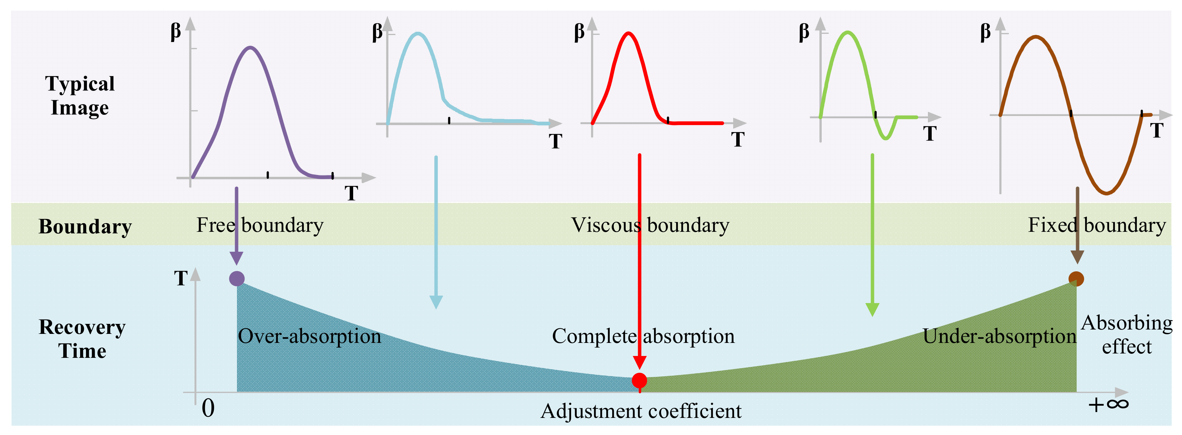
2.1. Basic Principles of the Viscous Boundary

Although the seismic wave can propagate freely in the infinite medium below the ground in the natural environment, the cost and efficiency of calculation necessitate that we intercept the infinite foundation medium as the calculation area artificially. Then, an artificial boundary is formed outside the intercepted area. The seismic wave will reflect at the boundary due to improper artificial boundary, which makes the seismic wave unable to transmit freely in the calculation area, and repeatedly stack and dissipate slowly within the model. For the research object, seismic waves’ superposition will seriously disturb or amplify the seismic response of structures, leading to an inaccurate or even wrong dynamic analysis. Therefore, the artificial boundary type and parameters can effectively influence the accuracy of structural seismic response analysis. Thus, in this paper, a viscous boundary is constructed in the PDEM, making the calculation results closer to the actual earthquake conditions than with a fixed boundary. The traditional advantages of the PDEM still exist in the dynamic structural analysis of the above implementation.

Unlike the continuum model such as the FEM, the PDEM model boundary is usually composed of spherical particles with different radii, making the PDEM model boundary surface uneven. According to the continuum theory, the principles equation of viscous boundary should be appropriately modified to be converted to a discrete material [18]. According to the continuum mechanics theory, the calculation formula of stress applied by the viscous boundary is given as follows:

$$\left\{\begin{array}{l}\sigma =C_{\mathrm{P}}\gamma {\nu }_{\mathrm{nor}}\\ \tau =C_{\mathrm{S}}\gamma {\nu }_{\mathrm{she}}\end{array}\right.$$

(1)

where $\sigma$ and $\tau$ are normal and shear forces applied to the viscous boundary, respectively. $C_{\mathrm{P}}$ and $C_{\mathrm{S}}$ are P-wave and S-wave velocities of the material, respectively. $\gamma$ is the density, while ${\nu }_{\mathrm{nor}}$ and ${\nu }_{\mathrm{she}}$ are normal and shear vibration velocities of the particles on the viscous boundary. For the PDEM, Equation (8) unit length stress of the viscous boundary in the FEM should be rewritten as the force for a single particle so that the viscous boundary for the PDEM is installed. For the reflection boundary, the external force applied by the viscous boundary can be described as:

$$\left\{\begin{array}{l}{F}_{\mathrm{nor}}=-F_{\mathrm{app}.\mathrm{nor}}-2R\xi \gamma C_{\mathrm{P}}{\nu }_{\mathrm{nor}}\\ F_{\mathrm{she}}=-F_{\mathrm{app}.\mathrm{she}}-2R\eta \gamma C_{\mathrm{S}}{\nu }_{\mathrm{she}}\end{array}\right.$$

(2)

where $F_{\mathrm{nor}}$ and $F_{\mathrm{she}}$ are the normal and shear forces applied to the boundary particles, respectively, while their directions are referred to the extension direction of the boundary interface. $F_{\mathrm{app}.\mathrm{nor}}$ and $F_{\mathrm{app}.\mathrm{she}}$ are the normal and shear forces provided by the wall under static state, respectively, and $R$ is the particle radius. Considering the dispersion effect of the seismic wave and the random distribution of particle radius, the adjustment coefficients of the longitudinal wave $\xi$ and the Transverse wave $\eta$ are introduced to achieve the best absorbing effect of the viscous boundary [18]. These are the governing equations of the viscous boundary in the PDEM.

To avoid the interaction between the Wall force and the viscous boundary force, the external force by programming replaces the application of the Wall force and the viscous boundary force. Therefore, in the dynamic calculation, the wall in the balance calculation process needs to be deleted, so the $F_{\mathrm{app}.\mathrm{nor}}$ and $F_{\mathrm{app}.\mathrm{nor}}$ are calculated and reapplied. To maintain the overall balance of the PDEM model, it is necessary to impose a constraint by commanding the particles at the boundary after the wall is deleted. For the PDEM, the forces acting on a single particle can be divided into indirect contact force ${\mathit{F}}_{\mathrm{contact}}$, gravity force ${\mathit{G}}_{\mathrm{gravity}}$, and external force ${\mathit{F}}_{\mathrm{app}}$ [1]. The resultant force is the unbalanced force of the sphere as follows:

$${\mathit{F}}_{\mathrm{unbal}}={\mathit{F}}_{\mathrm{contact}}+{\mathit{G}}_{\mathrm{gravity}}+{\mathit{F}}_{\mathrm{app}}$$

(3)

Since the unbalanced force of the particles on the PDEM boundary is zero after the initial equilibrium calculation, the force applied by the command on boundary particles can be calculated as follows:

$${\mathit{F}}_{\mathrm{app}}=\left[\begin{array}{l}{F}_{\mathrm{app}.\mathrm{nor}}\\ F_{\mathrm{app}.\mathrm{she}}\end{array}\right]=-{\mathit{F}}_{\mathrm{contact}}-{\mathit{G}}_{\mathrm{gravity}}$$

(4)

Moreover, for the input boundary of the seismic wave, the external force applied by the viscous boundary can be calculated as:

$$\left\{\begin{array}{l}{F}_{\mathrm{nor}}=-F_{\mathrm{app}.\mathrm{nor}}-2R{\xi }_{\mathrm{inp}}\gamma C_{\mathrm{P}}\left({\nu }_{\mathrm{nor}}-2{\nu }_{\mathrm{wave}.\mathrm{P}}\right)\\ F_{\mathrm{she}}=-F_{\mathrm{app}.\mathrm{she}}-2R{\eta }_{\mathrm{inp}}\gamma C_{\mathrm{S}}\left({\nu }_{\mathrm{she}}-2{\nu }_{\mathrm{wave}.\mathrm{S}}\right)\end{array}\right.$$

(5)

where ${\xi }_{\mathrm{inp}}$ and ${\eta }_{\mathrm{inp}}$ are the longitudinal wave and Transverse wave adjustment coefficients at the input boundary, respectively. ${\nu }_{\mathrm{wave}.\mathrm{P}}$ and ${\nu }_{\mathrm{wave}.\mathrm{S}}$ are normal and shear vibration velocities of the particles on the input boundary. Since half of the input wave energy will be absorbed by the viscous boundary, the coefficient equals 2 [24].

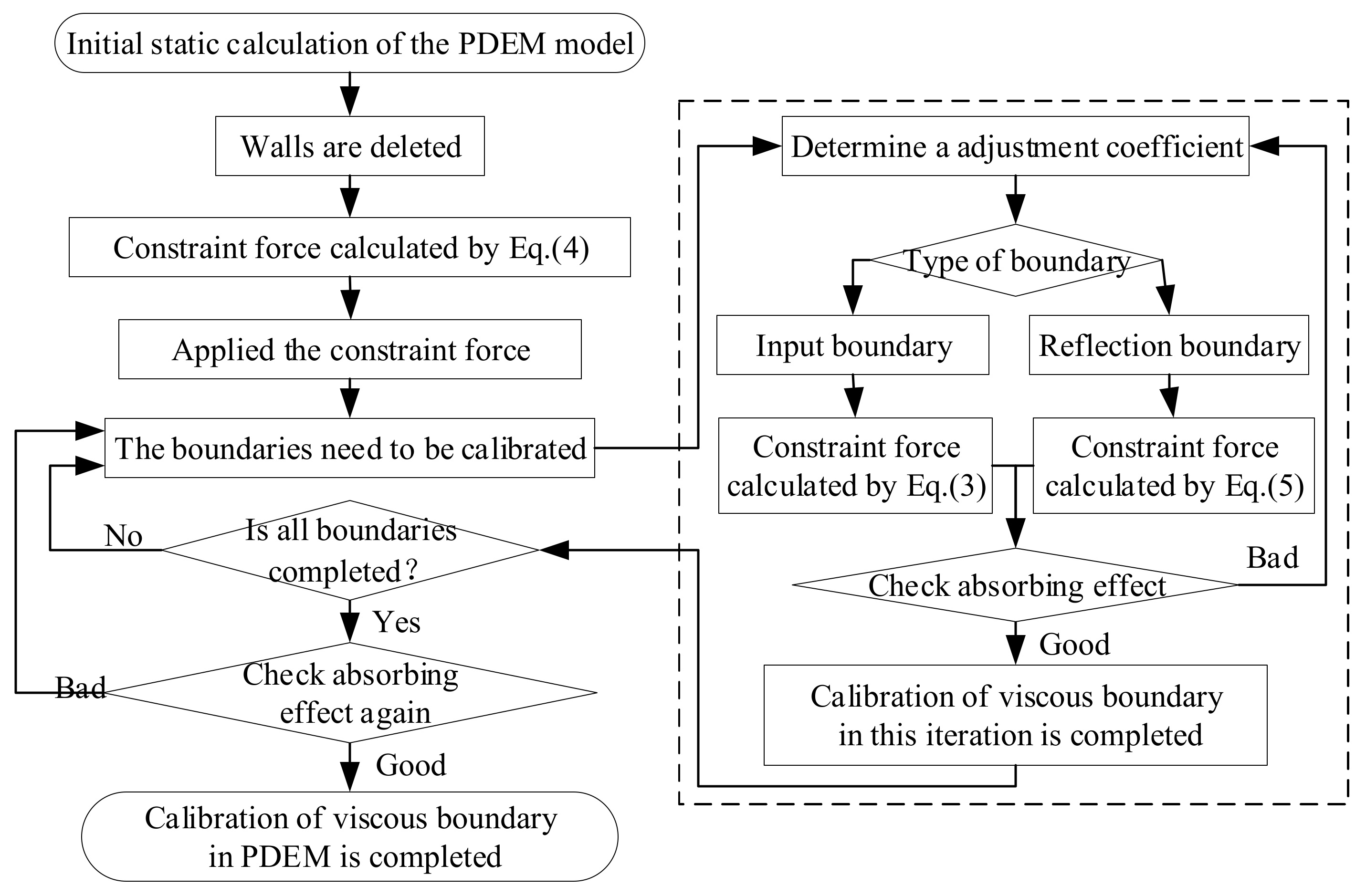
2.2. Application of Viscous Boundary in the PDEM

The disk and wall are essential elements in the PDEM. The rigid disk is allowed to overlap to simulate the structural deformation. The rigid wall is usually utilized as a boundary. In the previous dynamic response analysis with the PDEM, the vibration or seismic wave was directly applied to the wall [31] or several layers of the disk near the wall [8], closer to the fixed boundary. The viscous boundary application should be based on the static calculation, and then applying the corresponding viscous boundaries.

Figure 1 shows the flow chart of applying the viscous boundary in the PDEM, where its steps are given. (a) The calculation is completed to obtain the initial stress field under gravity. (b) The wall restricting the displacement of the particles on the boundary is removed; the constraint force is then calculated and applied to the particle to stabilize the PDEM model after the walls are deleted. (c) Indicate whether the boundary is an input boundary or a reflection boundary. The constraint force is then determined according to (4) or (5) to install the damper at the viscous boundary. (d) The adjustment coefficients of the longitudinal wave and Transverse wave of each boundary are calibrated in the PDEM model. (e) Since the subsequent change of the adjustment coefficient can influence the calibrated adjustment coefficients, each boundary’s absorbing effect will be rechecked after a calibration operation round until all the boundaries meet the absorbing effect requirements. The calculation and application of the viscous boundary are realized by programming in the PFC5.0 software. Since the influence of boundary location, boundary type, seismic wave type, and calibration sequence should be considered in determining the adjustment coefficient of the viscous boundary, the whole calibration process is usually complicated and requires a lot of calculations and practical experience. Therefore, it is necessary to develop a fast and efficient method for calibrating the adjustment coefficients in the PDEM.

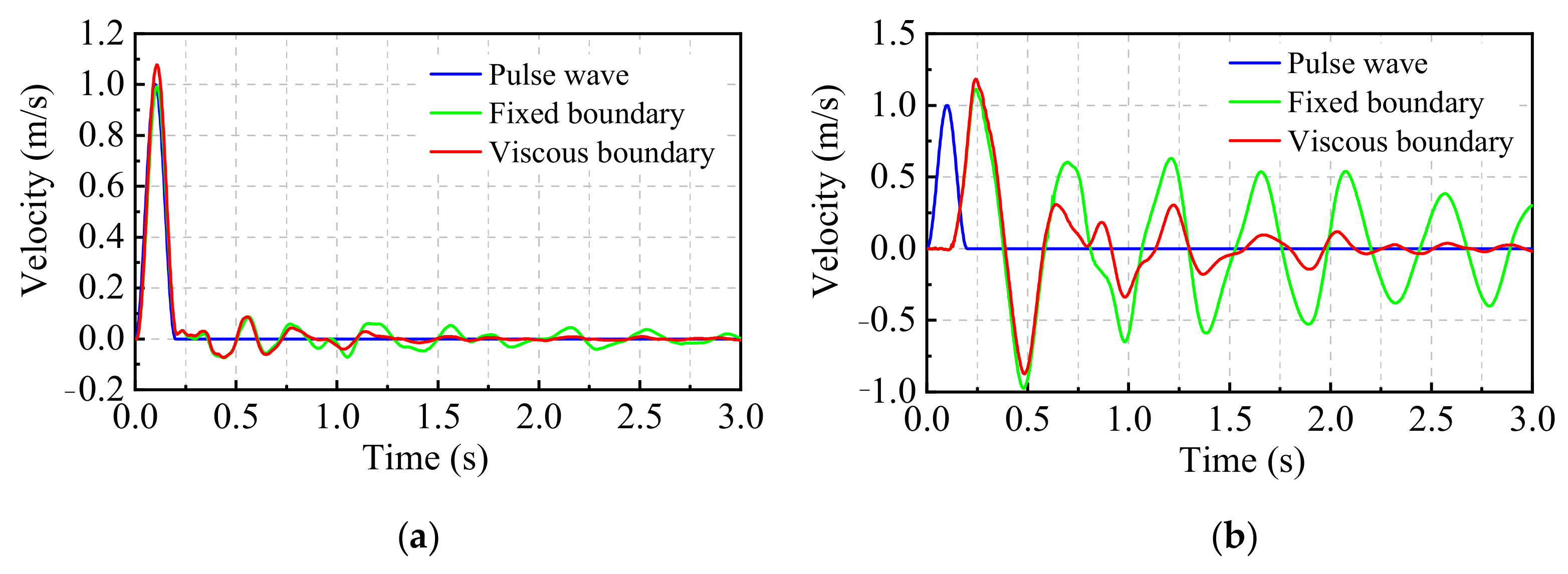
2.3. Verification of the Viscous Boundary in the PDEM

A strip PDEM model of the foundation is established like the Hopkinson bar test to verify the correctness of the viscous boundary in the PDEM and its absorbing effect. As shown in Figure 2, the foundation model size is 1000 × 50 m (horizontal × vertical). The model can remain stable after the wall is deleted if the vertical and horizontal constraints are applied to the bottom, and the left and right boundaries, respectively. To prevent the bond between particles from seismic damage, the particle’s bond strength should be increased appropriately. Meanwhile, five monitoring points (T1–T5) are adjusted to monitor the dynamic response of the model.

During excitation, a horizontal periodic harmonic longitudinal wave pulse is applied to the left boundary of the model, which is given by:

$$P_{\mathrm{vel}}=\left\{\begin{array}{ll}0.5A\left(1-\cos \left(2\pi t/T\right)\right)& \left(t\le T\right)\\ 0& \left(t>T\right)\end{array}\right.$$

(6)

where $P_{\mathrm{vel}}$ is the horizontal wave velocity of the particle at the input boundary. $A$ is the pulse wave amplitude, where its value is considered as 1 m/s in this paper. $T$ is the pulse cycle, and its value is chosen as 0.2 s in this paper. After applying the above pulse wave to the PDEM model, the internal response with a fixed or viscous boundary can be monitored to verify the viscous boundary effect in the PDEM.

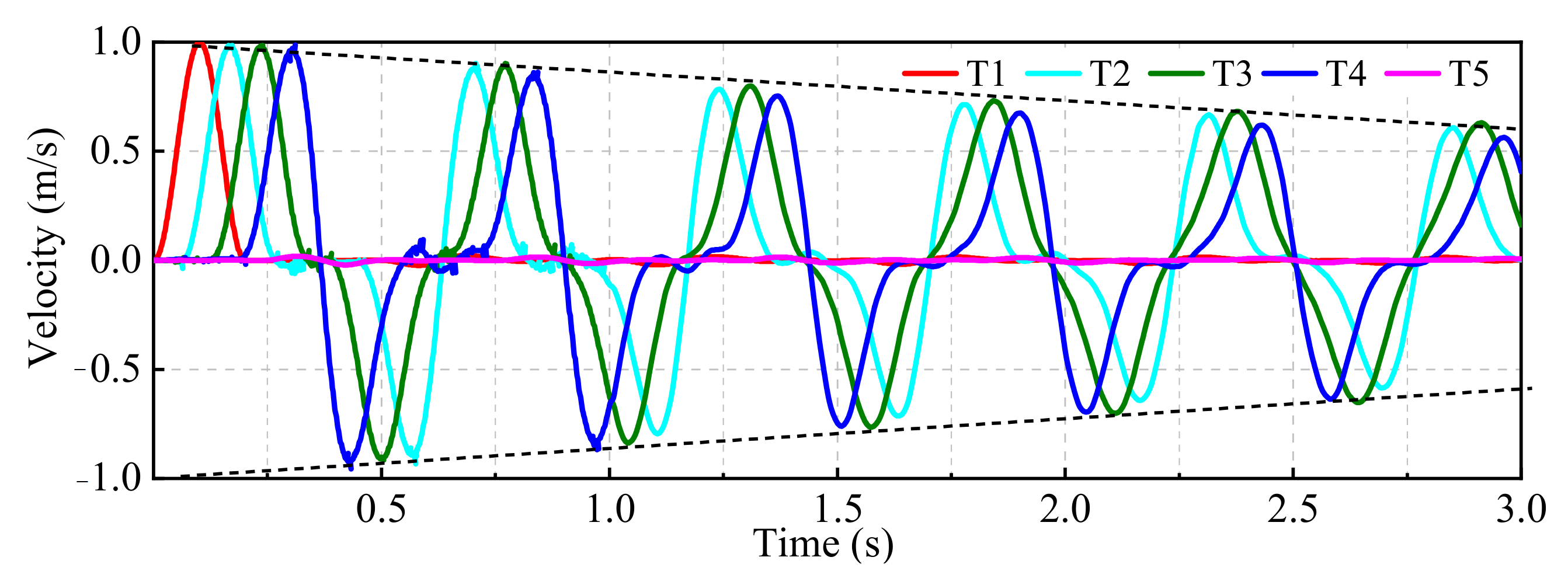
2.3.1. Dynamic Response Analysis of the Fixed Boundary

By fixing the particle’s velocity at 0 m/s or the particle’s position, the left and right boundaries of the PDEM model become fixed boundaries. Then, a pulse wave is applied to the left boundary (see Figure 3). The variation of horizontal velocity with time at T1–T5 monitoring points is shown in Figure 4.

(1) The T1 monitoring point is close to the left boundary. Its horizontal velocity history is similar to that of the pulse wave because the left boundary is the input boundary of the pulse wave in the DEM model. The T1 monitoring point starts to vibrate immediately under the pulse wave action to reach a peak velocity of 1 m/s at 0.1 s. Then, the T1 monitoring point’s velocity recovers to 0m/s with the end of the pulse wave after 0.2 s. Since the T5 monitoring point is located at the right fixed boundary, its velocity is always kept at 0 m/s.

(2) The time required from the exciter to peak is about 0.1s for T2, T3, and T4 monitoring points, that is T/2. During the pulse wave propagation, the velocity peak value of monitoring points decreases gradually. Then, T4, T3, and T2 monitoring points’ velocities become negative, indicating that the pulse wave is reflected by the right fixed boundary and its propagated direction switches from right to left. After that, T2, T3, and T4 monitoring points velocities showed positive and negative periodic transitions, illustrating that the pulse wave was reflected continuously by the left and right fixed boundary. This means that the pulse wave can propagate back and forth in the model with the fixed boundary and cannot dissipate quickly.

(3) The horizontal velocity extremum of T2, T3, and T4 monitoring points showed a linear attenuation trend with time, implying that the seismic wave energy gradually lost in the foundation’s propagation process.

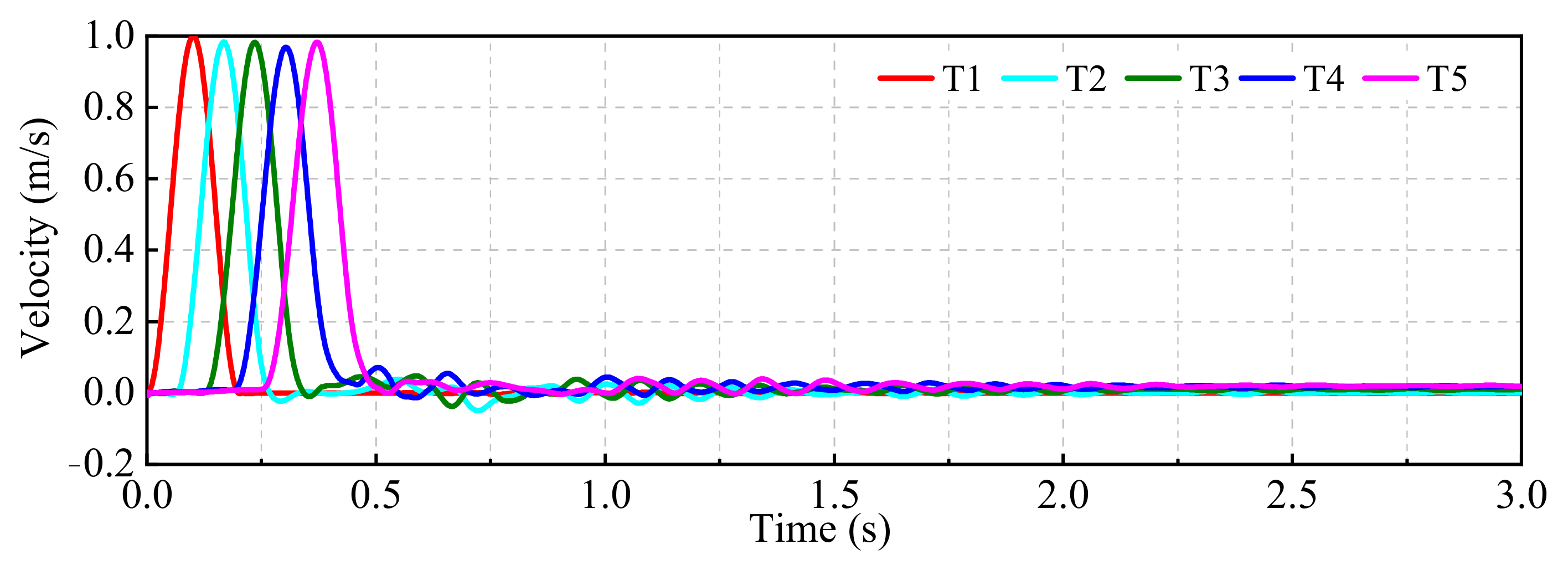
2.3.2. Dynamic Response Analysis of the Viscous Boundary

To verify the viscous boundary’s absorbing effect, the left boundary of the PDEM model is considered the fixed boundary, while the right reflecting boundary is chosen as the viscous boundary. As shown in Figure 5, the pulse wave is applied from the left boundary. According to the application method of the viscous boundary in Section 3.2, the longitudinal wave adjustment coefficient of the viscous boundary at the right boundary is 0.91, and the horizontal velocity history of the T1–T5 monitoring points is presented in Figure 6.

When the right reflection boundary is viscous, the vibration of the T1, T2, T3, and T4 monitoring points is similar to that of the fixed boundary in the first period. Then, each measuring point’s velocity decreases rapidly and fluctuates slightly in the range of −0.05~0.06 m/s and gradually approaches 0 m/s. Figure 6 shows that most of the pulse wave is absorbed by the right viscous boundary, which has a desirable absorbing effect. Besides, some vibration still exists in the DEM model, which may be due to the fixed boundary’s uneven surface profile at the top and bottom. Therefore, there is weak reflection and interference on the fixed boundary at the top and bottom during the pulse wave transmission, causing the pulse wave to be entirely absorbed by the viscous boundary in a short time. Simultaneously, since the right viscous boundary is not constrained, a change in the T5 monitoring point’s velocity can be observed.

Besides, when the pulse wave’s input boundary is viscous, the adjustment coefficient of the longitudinal wave is 0.65, indicating an excellent absorbing effect. According to the above analysis and references [24,25], it is feasible to set the viscous boundary in the PDEM. Compared with the fixed boundary, the viscous boundary shows a strong absorbing effect such that the pulse wave can freely spread out of the PDEM boundary. However, determining the adjustment coefficient of the viscous boundary is still a complicated process.

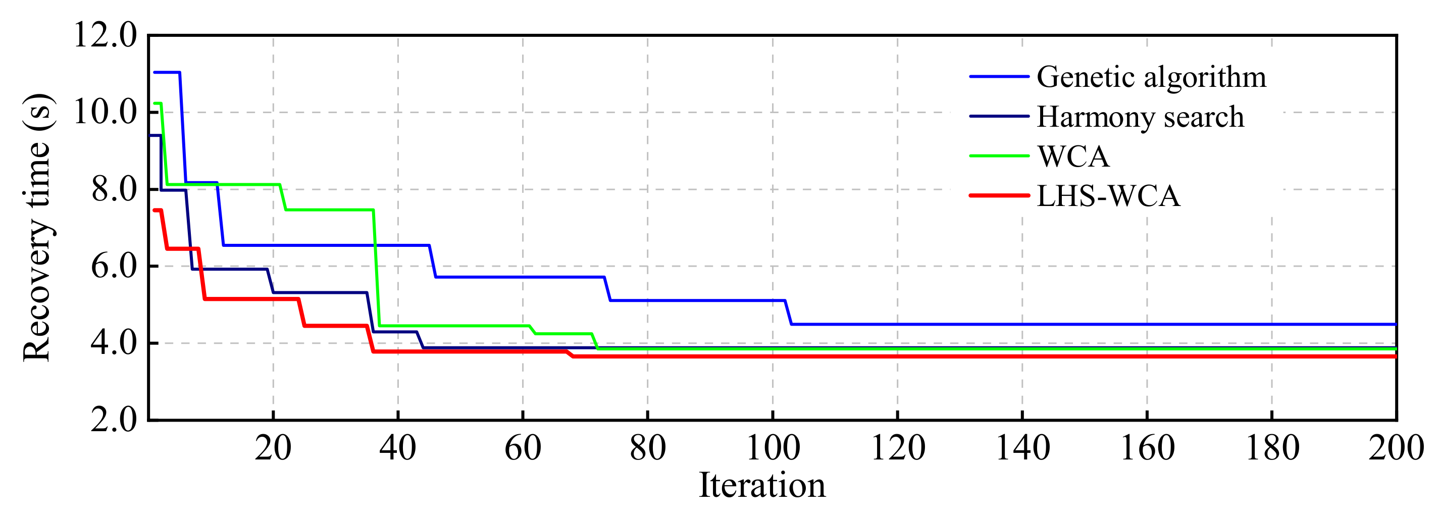
3. Establishment of LHS-WCA Algorithm

3.1. Basic Principles of the WCA

After a rainfall, land water always flows downward due to gravity, continuously merges with other rivers, and finally, at the lowest elevation, flows into the sea. Inspired by the water cycle process in nature, Eskandardeng et al. [29] proposed the WCA, a heuristic algorithm based on population in 2012. The WCA abstractly simulates the water cycle process of rainfall forming streams, streams merging into rivers, rivers flowing into the sea, and evaporation reforming as rainfall in nature. To find the approximate optimal solution, the WCA guides the flow concentration by the fitness, and it can simulate the water constantly searching for the path to the sea. Evaporation and rainfall are used to jump out of the local optical solution in this process. The advantages of the WCA have been gradually proved in the fields of mathematics [32], mechanical engineering [33], electrical engineering [34], control engineering [35], structural engineering [36], and civil engineering [37]. The flow chart of the WCA is shown in Figure 7, which shows that the calculation steps of WCA are as follows:

(1) Initial parameters of WCA are set, including initial population number $N_{pop}$, the number of rivers and seas $N_{sr}$, the number of variables to be optimized $N$, upper limit $UB$, lower limit $LB$, the speed of the adjusting parameter $C$, the readjust range parameter $u$, the evaporation judge parameter $d_{max}$, the maximum iterations $I{T}_{max}$.

(2) The initial population $\left[Water\right]$ is generated as shown in Equation (1), of which the individuals are called $Raindrop$. The fitness of the initial population is calculated, and the $Raindrop$ is divided into $X_{sea},X_{river}$, $X_{stream}$. According to the fitness of the river and the sea, the number of streams and stream individuals connected with them are determined [38,39].

$$\left[\mathit{W}\mathit{a}\mathit{t}\mathit{e}\mathit{r}\right]=\left[\begin{array}{c}Raindro{p}_1\\ Raindro{p}_2\\ ⋮\\ Raindro{p}_{N_{pop}}\end{array}\right]=\left[\begin{array}{c}{X}_{sea}\\ X_{river,1}\\ X_{river,2}\\ ⋮\\ X_{stream,1}\\ X_{stream,2}\\ ⋮\end{array}\right]=\left[\begin{array}{ccc}{x}_1^1& \cdots & x_N^1\\ ⋮& \ddots & ⋮\\ x_1^{N_{pop}}& \cdots & x_N^{N_{pop}}\end{array}\right]$$

(7)

(3) In the $t+1$ iterative calculation, for the $i\mathrm{th}$ stream flowing to the river, its position is determined according to Equation (8). For $i\mathrm{th}$ stream flowing to the sea, its position is determined according to Equation (9). For $i\mathrm{th}$ river flowing to the sea, its position is determined according to Equation (10). If each new position of an individual is better than its flowing object, the others’ positions are exchanged.

$$X_{stream,i}\left(t+1\right)=X_{stream,i}\left(t\right)+rand\times C\times \left(X_{river,i}\left(t+1\right)-X_{stream},i\left(t\right)\right)$$

(8)

$$X_{stream,i}\left(t+1\right)=X_{stream,i}\left(t\right)+rand\times C\times \left(X_{sea}\left(t+1\right)-X_{stream,i}\left(t\right)\right)$$

(9)

$$X_{river,i}\left(t+1\right)=X_{river,i}\left(t\right)+rand\times C\times \left(X_{sea}\left(t+1\right)-X_{river,i}\left(t\right)\right)$$

(10)

(4) The evaporation and rainfall conditions concur. With the iterative progress, rivers and streams gradually approach the sea. To enhance the searchability and prevent falling into the local optimal, evaporate and rainfall is carried out to form a new stream [29]. For streams flowing to the sea, rainfall is carried out near the sea to generate new streams, according to Equation (11). For rivers flowing to the sea, rainfall operation will be carried out in the entire basin to generate new streams, according to Equation (12). Then, the judgment condition of evaporation is updated according to Equation (13) and $d_{max}$.

$$X_{stream,i}^{new}\left(t+1\right)=X_{sea,i}\left(t\right)+\sqrt{u}\times randn\left(1,N\right), if \Vert X_{sea}-X_{stream,i}\Vert <d_{max}$$

(11)

$$X_{stream,i}^{new}\left(t+1\right)=LB+rand\times \left(UB-LB\right), if \Vert X_{sea}-X_{river,i}\Vert <d_{max}$$

(12)

$$d_{max}\left(t+1\right)=d_{max}\left(t\right)-\frac{d_{max}\left(t\right)}{I{T}_{max}}$$

(13)

(5) The iteration number is checked with the maximum iterations $I{T}_{max}$ to determine whether the stop condition realize. If not, steps (3) and (4) are repeated until the maximum iterations $I{T}_{max}$ are reached.

In other population algorithms, the individual moves directly to the optimal solution. In contrast, the individuals (stream) move indirectly to the optimal solution (ocean) because of the three-level architecture (stream, river, and sea) of the WCA, which can avoid falling into the local optimal solution. At the same time, in the search process, the individuals (streams) are guided to move towards better positions (rivers) to avoid searching inappropriate areas, which is conducive to the search efficiency of the WCA [40,41].

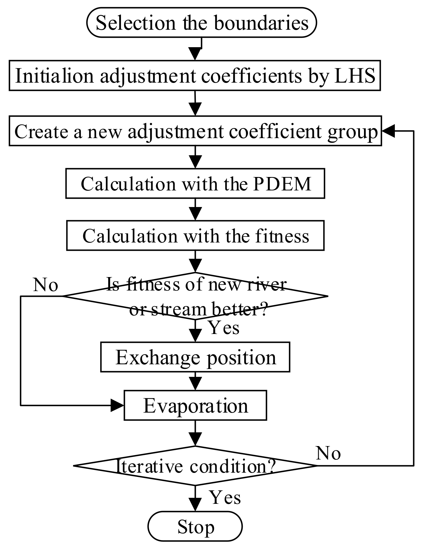
3.2. LHS-WCA Algorithm

From the above analysis, it can be seen that the search speed and quality of the WCA are greatly influenced by the quality of the initial population. Under the limited initial population, a more representative initial population within the upper and lower limits of variables should be constructed to improve the search speed and quality of WCA. Therefore, in this paper, Latin Hypercube Sampling (LHS) is introduced to establish the initial population of the WCA. The LHS divides each variable into several intervals with the same probability, and randomly selects sampling points in each interval to maintain the independence of samples and obtain higher sampling accuracy. Compared with other sampling algorithms, such as the random sampling method and orthogonal design method, the LHS has the advantages of wide application range, stable sampling estimation, better representativeness, and uniformity of samples [31,42]. Therefore, in this paper, the optimization algorithm LHS-WCA was established with Python to reduce the search time of the WCA, in which the smallest number of the initial population can represent a wider range of variable combinations.

4. Calibration Model of Adjustment Coefficients of the Viscous Boundary

4.1. The proposition of Calibration Problem

To attain the best absorbing effect, it is usually necessary to calibrate the viscous boundary’s adjustment coefficient. A large number of the FEM calculations demonstrate that the artificial boundary’s adjustment coefficient has good robustness, and the model shows a noticeable absorbing effect when the adjustment coefficient is within a value range shown in

Table 1. Range of adjustment coefficients for the viscous boundary.

Dimension	Type of Wave	Range	Recommendation [43]
2D	Transverse wave	0.35–0.65	1/2
	longitudinal wave	0.8–1.2	2/2
3D	Transverse wave	0.5–1.0	2/3
	longitudinal wave	1.0–2.0	4/3

.

For the PDEM, it is also necessary to find the optimal value of the adjustment coefficient to make a viscous boundary with the best absorbing effect due to the influence of the following factors. (a) In the PDEM model of an engineering structure, the boundary can reflect the seismic waves due to the particle distribution randomness and the particle size inconsistency. The random arrangement of particles in the PDEM and the non-uniform contact force can also affect seismic wave propagation. (b) Since the harmonic components of different frequencies have different phase velocities, the initial waveform is continuously scattering in the propagation process and forms the seismic wave’s dispersion effect. (c) Due to the engineering structure’s variable shapes, there are significant differences in the reflection angle and time of the seismic wave, leading to a complex superposition and dissipation of the seismic wave in the PDEM model. (d) Since there are various kinds of building materials with different properties in engineering structures, their elastic modulus and wave velocities are quite different. There is an apparent gap between the single wave velocity and the actual situation in the viscous boundary calculation. Therefore, for the PDEM model, the viscous boundary’s adjustment coefficient value is influenced by many factors, where cannot be determined by experience. Simultaneously, there is a nonlinear relationship between the longitudinal wave and Transverse wave adjustment coefficients of viscous boundaries. Thus, it is necessary to employ an optimization algorithm to calibrate the adjustment coefficients of the PDEM.

4.2. Well-Posedness of the Calibration Problem

Before solving the calibration problem, the solution’s well-posedness, including its existence, uniqueness, and stability, should be verified. First, the variation rule of the individual adjustment coefficient of the viscous boundary of the PDEM should be discussed. The different values of the adjustment coefficients indicate different magnitudes of the restraint applied to the boundary particles, leading to different absorption effects of the viscous boundary (see Figure 8). When the adjustment coefficient is less than the optimal value, the constraint force on the boundary is less than the particles’ force by the fluctuation, leading to incomplete absorption of the viscous boundary, and the residual fluctuation will cause a recurrence of reflection and interference within the model. If the adjustment coefficient reaches its minimum value (zero), the artificial boundary appears as a free boundary. When the adjustment coefficient is greater than the optimal value, the constraint force is greater than the particle’s force by the fluctuation, and the excess constraint force will cause new vibration. If the adjustment coefficient is infinitely large, the artificial boundary appears as a fixed boundary. Therefore, for a single viscous boundary, there is an optimal adjustment coefficient that can entirely absorb seismic waves, serving as the critical value for over- and under-absorption [25]. For a single viscous boundary, the time to restore to the static state generally decreases first and then increases with the adjustment coefficient’s gradual increase, which is easy to obtain. Thus, the optimal adjustment coefficient can make the PDEM model in the static state again in the shortest time. For the actual complex PDEM model, the recovery time is affected by the model size, boundary conditions, particle arrangement, and other factors, so the accurate recovery time can not be obtained directly. However, there must be a unique set of adjustment coefficients of viscous boundaries for multiple viscous boundaries, making the best absorbing effect for the PDEM model [25]. Therefore, the calibration analysis of adjustment coefficients of viscous boundaries is well-posed.

4.3. Feasibility and Construction of the Calibration Model

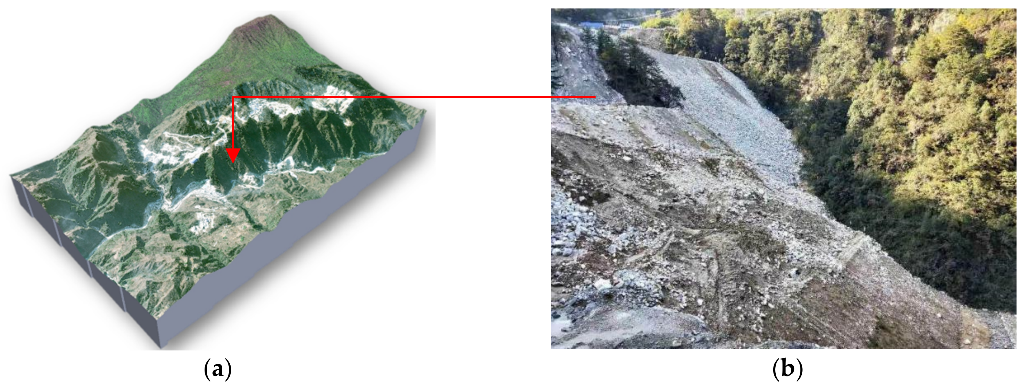
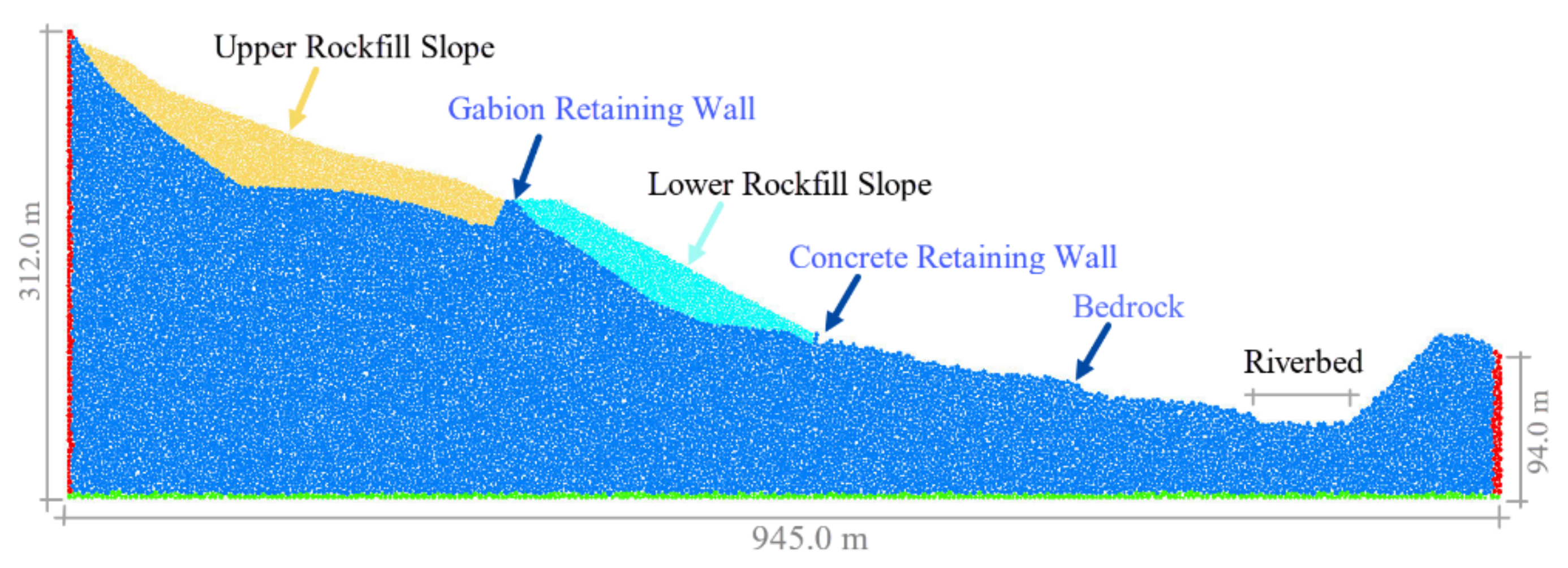
According to the above analysis, the nonlinear relationship between adjustment coefficients of the PDEM makes it challenging to quickly and accurately determine the adjustment coefficients of the viscous boundaries. On the other hand, the variation law of the viscous boundary’s adjustment coefficient ensures the existence and uniqueness of the calibration problem solution. Therefore, the adjustment coefficients can be uniquely determined in theory according to the dynamic response of the PDEM model. In this paper, the LHS-WCA algorithm with global search ability is introduced to construct the calibration model of the adjustment coefficients, which can calibrate the adjustment system array according to the dynamic response of the DEM, where its objective function is given by:

$$S_{\mathrm{vis}}\left(x_{\mathrm{RP}},x_{\mathrm{RS}},x_{\mathrm{LP}},x_{\mathrm{LS}},x_{\mathrm{BP}},x_{\mathrm{BS}},\cdots ,x_M\right)=\min \left\{\frac{1}{q}{\displaystyle \sum _{i=1}^q\left[TimeDE{M}_i\left(x_{\mathrm{RP}},x_{\mathrm{RS}},x_{\mathrm{LP}},x_{\mathrm{LS}},x_{\mathrm{BP}},x_{\mathrm{BS}},\cdots ,x_M\right)\right]}\right\}$$

(14)

where $x_{\mathrm{RP}},x_{\mathrm{RS}},x_{\mathrm{LP}},x_{\mathrm{LS}},x_{\mathrm{BP}},x_{\mathrm{BS}},\cdots ,x_M$ are $M$ adjustment coefficients of viscous boundaries to be calibrated, including the longitudinal wave and transverse wave adjustment coefficients of each viscous boundary. $q$ is the number of monitoring points arranged near the boundaries. $TimeDE{M}_i$ is the time required for the measuring points to drop below the permissible speed.

The flow chart of the LHS-WCA based calibration model of adjustment coefficients of viscous boundaries in the PDEM model is shown in Figure 9, and its specific implementation steps are as follows:

(1) The engineering structure characteristics, the PDEM model, the seismic wave’s input mode, and the type of seismic wave are employed to determine the artificial boundaries, which should be calibrated.

(2) Since the uniformity and representativeness of initial samples directly affect the WCA algorithm’s convergence rate, the LHS is utilized to generate multiple groups of adjustment coefficients of the viscous boundary within the parameter range. Then, the PDEM is adopted to calculate the total time required for each monitoring point to drop below the acceptable velocity, and it is also the fitness of the corresponding adjustment coefficient group. This completes the initialization population of the WCA.

(3) New adjustment coefficient groups will generate in the WCA’s calibration process, and the PDEM results are employed to obtain the corresponding fitness. If the new adjustment coefficient group’s fitness is superior to the worst, the new adjustment coefficient group is exchanged to update the river and sea in the WCA; Otherwise, the next step is directly executed.

(4) The iteration time is checked to determine whether the calculation needs to stop. If not, step (3) is repeated until the iteration time reaches its final value; Otherwise, the optimal parameter group and its fitness are chosen as the calibration results of the adjustment coefficient of the viscosity boundary in the PDEM model.

5. Case Study

A pumped storage power station is responsible for peak regulation, countering power shortfalls, frequency modulation, phase modulation, and an emergency standby of the power system with an average annual power generation of 2.341 billion kW·h. In the engineering construction, several platforms should be constructed, where the construction materials are discarded dregs of the road. One is a rockfill slope with a maximum height difference of 199.8 m. This rockfill slope not only has a large slag scale but also has a direct impact on the overall safety of the project (see Figure 10).

To verify the influence degree and range of the rockfill slope instability under the most unfavorable conditions, the PDEM model is established for the most unfavorable 2D section of the rockfill slope in the operation period by comprehensively considering the original topography, slope shape, and slag characteristics of the rockfill. Compared with the 3D model, the 2D PDEM model ignores the rolling and collision buffering effect, which increases the safety margin of the rockfill slope and makes the 2D model more unfavorable than the 3D one. In the operation period, the seismic condition has an unfavorable influence on slope stability. As shown in Figure 11, the rockfill slope’s PDEM model is established with the viscous boundary to investigate the instability process under seismic conditions. Simultaneously, a total of 37 monitoring points are arranged in the PDEM model to master the wave absorbing effect of the viscous boundary and the seismic response of the rockfill slope (see Figure 12).

The PDEM model size of the rockfill slope is 945 × 312 m (horizontal × vertical). According to the grain-size distribution curve obtained from the field investigation, after cutting off the small size, the particle size of 0.2–0.7 m is used to simulate the rockfill in the slope. For the bedrock in the slope, a 5 m particle size is adopted to transmit seismic waves. There are 12,798 disks in the bedrock, 4614 disks in the rockfill slope above the gabion retaining wall, and 2667 disks in the rockfill between the gabion retaining wall and concrete retaining wall. The horizontal velocity is positive along the slope. Spherical particles simulate the foundation to simulate the seismic propagation in the foundation and the foundation force on the rockfill slope, while the left, right, and bottom boundaries of the PDEM model are considered viscous boundaries.

5.1. Calibration of Microscopic Parameters of the Rockfill

For the PDEM, the selection of the microscopic contact model and its parameters has an obvious and direct influence on the simulation results. Therefore, before the dynamic response analysis with the PDEM, the microscopic contact model of the rockfill should be selected, and its microscopic parameters should be accurately calibrated. Although there is no cohesive force between the rockfill, the irregular shape produces an apparent biting force between the rockfill so that the contact bond model can be adapted to the simulation rockfill. Field sampling and large-scale triaxial tests are performed for the rockfill slope to attain accurate and reliable microscopic parameter values. The specimen size is Φ300 × 600 mm, and the shear rate is 0.4 mm/min with 200 kPa, 500 kPa, 800 kPa, 1200 kPa confining pressures. The deformation characteristic curve calibrates the rockfill’s microscopic parameters using the calibration method proposed in [44]. Accordingly, the normal stiffness $k_n=3.5\mathrm{MN}/\mathrm{m}$, shear stiffness $k_s=2.6\mathrm{MN}/\mathrm{m}$, friction coefficient $\mu =0.09$, normal bond force $b_n=2.2\mathrm{kN}$, and shear bond force $b_s=1.6\mathrm{kN}$ of rockfill particles are determined.

In this paper, the parallel bond model is utilized to simulate the bedrock. According to [17], the following relationship can be written between the elastic modulus and the longitudinal wave velocity for the rock

$$\left\{\begin{array}{l}{C}_{\mathrm{P}}=\sqrt{\frac{E_{\mathrm{d}}(1-{\mu }_{\mathrm{d}})}{\rho (1+{\mu }_{\mathrm{d}})(1-2{\mu }_{\mathrm{d}})}}\\ C_{\mathrm{S}}=\sqrt{\frac{E_{\mathrm{d}}}{\rho (1+{\mu }_{\mathrm{d}})}}\end{array}\right.$$

(15)

where $E_{\mathrm{d}}$ and ${\mu }_{\mathrm{d}}$ are the dynamic elastic modulus and the dynamic Poisson’s ratio, respectively. $\rho$ is the density. The wave velocity and the Poisson’s ratio can be determined according to the bedrock type. The microscopic parameters can then be determined according to the weathering, fracture, empirical range of longitudinal wave velocity, the ratio of the longitudinal wave to Transverse wave, and the relationship between dynamic elastic modulus and elastic modulus. Since the rockfill slope’s bedrock is marble, the weak weathering depth is generally higher than 15~20 m. Furthermore, the rock mass is relatively complete, and fracture development is general. Therefore, the bedrock’s microscopic parameters in the rockfill slope are determined as macroscopic elastic modulus $E_{\mathrm{ball}}=4\mathrm{GPa}$ and stiffness ratio $K=k_n/k_s=1.67$.

5.2. Calibration of Adjustment Coefficients of the Viscous Boundary and Its Effect Analysis

To determine adjustment coefficients of viscous boundaries, a periodic pulse wave is applied to the bottom boundary of the rockfill slope’s PDEM model, and the proposed LHS-WCA based calibration model of adjustment coefficients is utilized. The calibration results are shown in

Table 2. Values of adjustment coefficients of viscous boundaries in the rockfill slope.

		Longitudinal Wave		S-Wave
Adjustment coefficients	Boundary	Range	Calibration results	Range	Calibration results
	Left (reflection)	[0.5, 2.0]	0.97	[0.2, 1.5]	0.65
	Right (reflection)	[0.5, 2.0]	0.96	[0.2, 1.5]	0.68
	Bottom (input)	[0.5, 2.0]	1.02	[0.2, 1.5]	0.61
Simulated wave velocity (m/s)		3512		1853

. The longitudinal wave adjustment coefficients are greater than the Transverse wave, following the understanding law of adjustment coefficients in the FEM. Besides, the distance between measuring points and the wave peak difference time is utilized to calculate the simulated wave velocity, and its closeness to the actual demonstrates the correctness of the bedrock’s microscopic parameters.

In the calibration process, the maximum iteration IT_max of the WCA algorithm is selected as 80 times, and the initial population size is 40 groups. At the same time, the sum of velocity recovery time of 8 monitoring points (1-1, 1-4, 1-8 on the left boundary; 5-1, 5-2 on the right boundary; 2-1, 3-1, 4-1 on the bottom boundary) is considered as the fitness of the corresponding adjustment coefficient of the viscous boundary. The convergence rate of the LHS-WCA is compared with other optimization algorithms in Figure 13. It can be seen that the computational efficiency of the LHS-WCA is obviously superior to the genetic algorithm and harmony search, and it can rapidly determine the optimal values of the adjustment coefficients. Compared with the WCA, the LHS-WCA significantly improves the search accuracy at the initial stage of the calculation and overall speed. When the iteration number reaches 44, the total recovery time reaches the minimum value of 3.654 s. Otherwise, in the process of calibration of adjustment coefficient of viscous boundary, the absorbing effect of model boundary is constantly adjusted, and the recovery time of monitoring points is continuously reduced. It shows that the calibration model established in this paper can achieve the best absorbing effect of the PDEM boundary in a short time via the LHS-WCA.

The typical measuring points in the artificial boundary and inside the bedrock are shown in Figure 14 through considering a fixed or viscous boundary in the PDEM model of the rockfill slope, while monitoring points 2-1 are located inside an artificial boundary, and monitoring points 2-4 are located inside the bedrock near the ground surface. It can be seen from Figure 14a that the pulse wave can dissipate rapidly and recover to 0 m/s at 1.34 s with the viscous boundary. Although the pulse wave is attenuated continuously on the fixed boundary, it is not easy to recover to the static state in a short time due to the repeated reflection. Therefore, the established viscous boundary has an excellent absorbing effect and effectively avoids reflection, echo, and seismic wave interference. It can be seen from Figure 14b that monitoring points 2-4 are always in the vibration state under the influence of reflected waves after the earthquake, while the attenuation amplitude is small. In the viscous boundary case, the 2-4 monitoring points and the bedrock’s interior can be restored to the static state quickly. Besides, compared with the dynamic response of the boundary, the interior DEM model’s dynamic response is greatly influenced by the artificial boundary conditions due to the “whiplash effect” and the superposition of reflected waves. In summary, after calibration of the adjustment coefficient by the LHS-WCA, the viscous boundary in the PDEM model can absorb the reflected wave and reproduce the natural dissipation process of vibration in the foundation, which improves the accuracy and reasonable dynamic response analysis of the rockfill slope.

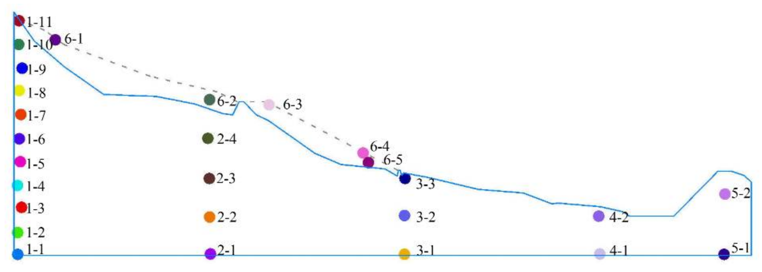
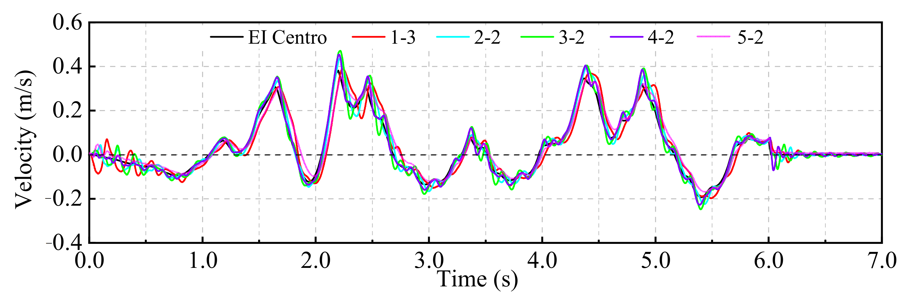
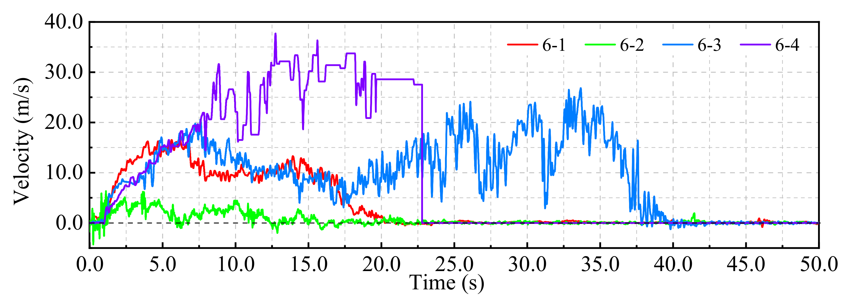
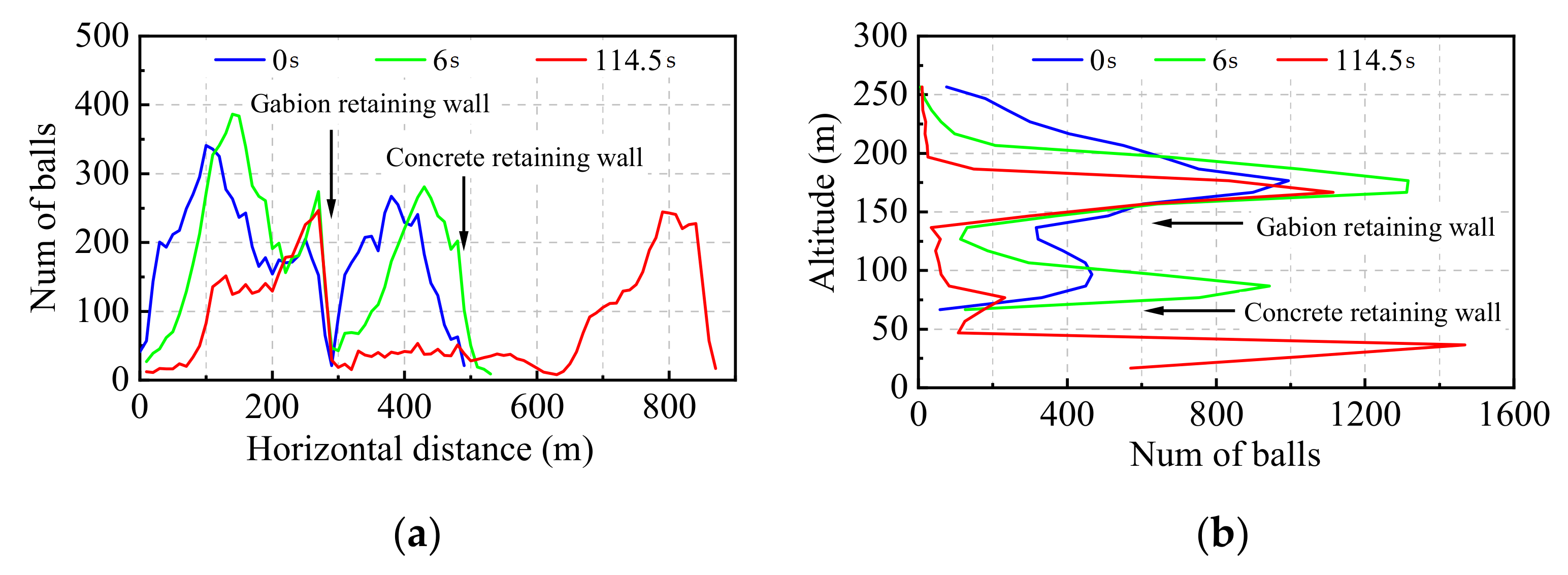
5.3. Time History Analysis of the Rockfill Slope

After calibrating the adjustment coefficients of the viscous boundary, the rockfill slope’s PDEM model is adopted to perform the time history analysis of the rockfill slope under seismic conditions. In general, since the vertical seismic wave has a more noticeable effect on the slope failure [45], the first 6 s of EI Centro seismic waves are applied to the viscous bottom boundary as a form of the Transverse wave. When the average unbalanced force ratio is less than 0.01, the instability evolution of the rockfill slope is completed. The entire process lasts 114.5 s, which takes 71 h and 23 min.

To evaluate the bedrock’s seismic response, a group of horizontal monitoring points in the bedrock and near the bottom of the model are selected. The horizontal velocity time history curve is shown in Figure 15. (a) The variation trend and the horizontal velocity law of each measuring point are similar to that of the seismic wave, indicating that the viscous boundary can effectively absorb the seismic wave. (b) In the initial stage, the velocity of monitoring points 1-3 and 5-2 fluctuates and remains relatively constant after 0.8 s. The possible reason is that the particles on the boundary need to adjust iteratively after the viscous boundary replaces the fixed boundary. (c) The maximum velocity of this monitoring point group is the peak velocity 0.47m/s of 3-3 monitoring point points at 2.22 s, which is about 1.30 times of the seismic wave. (d) Generally, when the velocity of monitoring points reaches its extreme value, the velocity of 3-2 monitoring points is the largest, followed by 2-2 and 4-2 monitoring points, while 1-3 and 5-2 monitoring points are the smallest. It shows that the particle velocity is small on the left and right sides of the PDEM model and large on the central section. (e) After the earthquake, each monitoring point’s velocity shows a small amplitude oscillation and gradually decreases and tends to 0 m/s after 7.1 s, indicating that the viscous boundary can absorb the seismic wave quickly. The viscous boundary in the PDEM model can simulate the natural and rapid dissipation process of the seismic wave in the foundation, establishing a foundation for accurate analysis of the rockfill slope’s seismic response.

To master the movement of rock blocks on the rockfill slope under seismic conditions, 6-1 and 6-2 monitoring points are arranged at the top and bottom of the upper slope, and 6-3 and 6-4 monitoring points at the top and bottom of the lower slope. The velocity-time history curve is shown in Figure 16. (a) The 6-1 stone at the top of the upper slope slides rapidly when the earthquake starts and then slows down under the block of the front of the upper slope. Thus, the velocity of 6-1 stone generally increases first, then becomes stable and stops at the upstream side of the gabion retaining wall after the 20 s. (b) The 6-2 block stone at the front of the upper slope slides downstream under the upper slope push, and it stays at the upstream side of the gabion retaining wall. The velocity of 6-2 stone always maintains a small value and shows a noticeable fluctuation. (c) The velocity of stones 6-3 at the top of the lower slope shows the sliding stage and accelerating sliding to the riverbed stage, reaching and staying at the riverbed in 41.2 s. (d) The movement speed of stones 6-4 on the lower slope increases continuously and crosses the concrete retaining wall. Moreover, it collides with the opposite bank at 23 s and stays at the riverbed.

Under the seismic condition, the rock stone distribution in the rockfill slope at the initial state (0 s), end of the earthquake (6 s), and final state (114.5 s) is shown in Figure 17. In the horizontal direction, the rockfill slope expands from 0–480 m in the initial state to 82–870 m after instability, while the peak number of the rockfill slope decreases significantly from 321 to 246. With the development of slope instability, the horizontal distribution curve moves to the right, indicating that the rockfill stone’s movement trend in the horizontal direction is to the downstream. Finally, it mainly accumulates in the upstream side of the gabion retaining wall and riverbed. In the vertical direction, the rockfill stones’ distribution curve moves downward, and the primary accumulation position changes from centralized distribution to distribution on the upstream side of the gabion retaining wall and riverbed. Therefore, after calibrating the adjustment coefficients, the movement characteristics of the rockfill slope and the distribution range of rock blocks after an earthquake can be accurately obtained with the PDEM model, establishing a strong foundation for dividing the dangerous area defining the earthquake influence scope.

6. Conclusions

To improve the accuracy of structural response dynamic analysis, a calibration model of the viscous boundary’s adjustment coefficient based on the LHS-WCA algorithm was established for the PDEM model in this study.

(1) The viscous boundary is constructed in the PDEM, and its application method was explained in detail. Like the Hopkinson bar test, a strip DEM model was utilized for the response analysis of the fixed and viscous boundaries. Accordingly, the feasibility of the viscous boundary in the PDEM was demonstrated.

(2) Then, since the adjustment coefficient could be affected by many factors and there was a nonlinear relationship between adjustment coefficients, the LHS-WCA algorithm was utilized to construct a calibration model of adjustment coefficients, which benefited from the well-posedness of adjustment coefficient calibration.

(3) Finally, the PDEM model with adjustment coefficients was adopted for a rockfill slope’s dynamic response analysis. The calibration of microscopic parameters of the rockfill and the adjustment coefficients of the viscous boundary were employed for an in-depth analysis of the movement and the distribution of the rockfill stone.

In a word, the LHS-WCA based calibration model could accurately determine the adjustment coefficients of the viscous boundary and effectively improve the simulation accuracy of dynamic response analysis with the PDEM. The accurate dynamic response results of PDEM could guide the design of structural seismic measures, which is of great significance to expand PDEM applications.

References

1. Cundall, P.A.; Strack, O.D. A discrete numerical model for granular assemblies. Geotechnique 1979, 29, 47–65. [Google Scholar] [CrossRef]
2. Liu, Q.; Sun, L.; Tang, X. Investigate the influence of the in-situ stress conditions on the grout penetration process in fractured rocks using the combined finite-discrete element method. Eng. Anal. Bound. Elem. 2019, 106, 86–101. [Google Scholar] [CrossRef]
3. Chen, Q.; Zhang, C.; Yang, C.; Ma, C.; Pan, Z. Effect of fine-grained dipping interlayers on mechanical behavior of tailings using discrete element method. Eng. Anal. Bound. Elem. 2019, 104, 288–299. [Google Scholar] [CrossRef]
4. Zhou, W.; Ma, G.; Liu, J.Y.; Chang, X.L.; Li, S.L.; Xu, K. Review of macro- and mesoscopic analysis on rockfill materials in high dams. Sci. Sin. Technol. 2018, 48, 1068–1080. (In Chinese) [Google Scholar] [CrossRef]
5. Maranha, D.N.E. Advances in Rockfill Structures; Springer: New York, NY, USA, 1991; pp. 11–23. [Google Scholar] [CrossRef]
6. Zhang, R.; Sun, Y.; Song, E. Simulation of dynamic compaction and analysis of its efficiency with the material point method. Comput. Geotech. 2019, 116, 103218.1–103218.19. [Google Scholar] [CrossRef]
7. Shahzadi, G.; Soulaïmani, A. Deep Neural Network and Polynomial Chaos Expansion-Based Surrogate Models for Sensitivity and Uncertainty Propagation: An Application to a Rockfill Dam. Water 2021, 13, 1830. [Google Scholar] [CrossRef]
8. Xiao, Q. Simulating the hydraulic heave phenomenon with multiphase fluid flows using cfd-dem. Water 2020, 12, 1077. [Google Scholar] [CrossRef] [Green Version]
9. Tang, C.L.; Hu, J.C.; Lin, M.L.; Yuan, R.M.; Cheng, C.C. The mechanism of the 1941 Tsaoling landslide, Taiwan: Insight from a 2D discrete element simulation. Environ. Earth Sci. 2013, 70, 1005–1019. [Google Scholar] [CrossRef] [Green Version]
10. Zhou, J.W.; Cui, P.; Fang, H. Dynamic process analysis for the formation of Yangjiagou landslide-dammed lake triggered by the Wenchuan earthquake, China. Landslides 2013, 10, 331–342. [Google Scholar] [CrossRef]
11. Chen, X.; Wang, H. Slope failure of noncohesive media modelled with the combined finite–discrete element method. Appl. Sci. 2019, 9, 579. [Google Scholar] [CrossRef] [Green Version]
12. Mendes, N.; Zanotti, S.; Lemos, J.V. Seismic Performance of Historical Buildings Based on Discrete Element Method: An Adobe Church. J. Earthq. Eng. 2018, 24, 1270–1289. [Google Scholar] [CrossRef]
13. Zhu, C.; Huang, Y.; Sun, J. Solid-like and liquid-like granular flows on inclined surfaces under vibration—Implications for earthquake-induced landslides. Comput. Geotech. 2020, 123, 103598. [Google Scholar] [CrossRef]
14. Zheng, Y.; Wang, R.; Chen, C.; Sun, C.; Zhang, W. Dynamic analysis of anti-dip bedding rock slopes reinforced by pre-stressed cables using discrete element method. Eng. Anal. Bound. Elem. 2021, 130, 79–93. [Google Scholar] [CrossRef]
15. Zhang, J.W.; Zhang, M.X.; Li, M.C.; Min, Q.L.; Shi, B.W.; Song, L.G. Nonlinear dynamic response of a CC-RCC combined dam structure under oblique incidence of near-fault ground motions. Appl. Sci. 2020, 10, 885. [Google Scholar] [CrossRef] [Green Version]
16. Karabulut, M.; Kartal, M.E. Seismic analysis of Roller Compacted Concrete (RCC) dams considering effect of viscous boundary conditions. Comput. Concr. 2020, 25, 255–266. [Google Scholar] [CrossRef]
17. Wang, Q.; Liu, Y.; Peng, G. Effect of water pressure on mechanical behavior of concrete under dynamic compression state. Constr. Build. Mater. 2016, 125, 501–509. [Google Scholar] [CrossRef]
18. Bao, H.; Hatzor, Y.H.; Xin, H. A new viscous boundary condition in the two-dimensional discontinuous deformation analysis method for wave propagation problems. Rock Mech. Rock Eng. 2012, 45, 919–928. [Google Scholar] [CrossRef]
19. Cui, F.P.; Xiong, C.; Wu, Q.; Xu, Q.; Li, N.; Wu, N.A.; Cui, L. Dynamic response of the Daguangbao landslide triggered by the Wenchuan earthquake with a composite hypocenter. Geomat. Nat. Hazards Risk 2021, 12, 2170–2193. [Google Scholar] [CrossRef]
20. Gu, J.; Zhao, Z.Y. Considerations of the discontinuous deformation analysis on wave propagation problems. Int. J. Numer. Anal. Met. 2009, 33, 1449–1465. [Google Scholar] [CrossRef]
21. Yang, C.W.; Zhang, J.J.; Zhang, M. A prediction model for horizontal run-out distance of landslides triggered by Wenchuan earthquake. Earthq. Eng. Eng. Vib. 2013, 12, 201–208. [Google Scholar] [CrossRef]
22. Yang, C.W.; Feng, N.; Zhang, J.J.; Bi, J.W.; Zhang, J. Research on time-frequency analysis method of seismic stability of covering-layer type slope subjected to complex wave. Environ. Earth Sci. 2015, 74, 5295–5306. [Google Scholar] [CrossRef]
23. Shi, C.; Zhang, Q.; Wang, S.N. Numerical Simulation Technology and Application with Particle Flow Code (PFC5.0); China Architecture and Building Press: Beijing, China, 2018; pp. 11–23. [Google Scholar]
24. Zhou, X.; Sheng, Q.; Cui, Z. Dynamic boundary setting for discrete element method considering the seismic problems of rock masses. Granul. Matter 2019, 21, 66. [Google Scholar] [CrossRef]
25. Zhou, X.T.; Sheng, Q.; Leng, X.L.; Fu, X.D.; Cui, Z. Viscous artificial boundary for seismic dynamic time-history analysis with granular discrete element method and its application. Chin. J. Rock Mech. Eng. 2017, 4, 154–165. (In Chinese) [Google Scholar] [CrossRef]
26. Zhou, X.T.; Wei, P.F.; Fu, X.D.; Li, L.H.; Xue, X.H. Dynamic Process and Mechanism of the Catastrophic Taihongcun Landslide Triggered by the 2008 Wenchuan Earthquake Based on Field Investigations and Discrete Element Method Simulations. Front. Earth Sci. 2021, 9, 710031. [Google Scholar] [CrossRef]
27. Wang, J.; Chi, S.; Shao, X.; Zhou, X. Determination of the mechanical parameters of the microstructure of rockfill materials in triaxial compression DEM simulation. Comput. Geotech. 2021, 137, 104265. [Google Scholar] [CrossRef]
28. Zhang, P.T.; Sun, X.J.; Zhou, X.J.; Zhang, Y.X. Experimental simulation and a Rapid reliable calibration method of rockfill microscopic parameters by considering flexible boundary. Powder Technol. 2021, 396, 279–290. [Google Scholar] [CrossRef]
29. Eskandar, H.; Sadollah, A.; Bahreininejad, A.; Hamdi, M. Water cycle algorithm—A novel metaheuristic optimization method for solving constrained engineering optimization problems. Comput. Struct. 2012, 110–111, 151–166. [Google Scholar] [CrossRef]
30. Shields, M.D.; Zhang, J.X. The generalization of Latin hypercube sampling. Reliab. Eng. Syst. Safe. 2016, 148, 96–108. [Google Scholar] [CrossRef] [Green Version]
31. Yang, Z.P.; Lai, Y.L.; Liu, S.L.; Tian, X.; Hu, Y.X.; Ren, S.P. Dynamic stability and failure mode of slopes with overlying weak rock mass under frequent micro-seismic actions. Chin. J. Geotech. Eng. 2019, 41, 131–140. (In Chinese) [Google Scholar] [CrossRef]
32. Qiao, S.; Zhou, Y.; Zhou, Y.; Wang, R. A simple water cycle algorithm with percolation operator for clustering analysis. Soft Comput. 2016, 23, 4081–4095. [Google Scholar] [CrossRef]
33. Mahdavi-Nasab, N.; Abouei Ardakan, M.; Mohammadi, M. Water cycle algorithm for solving the reliability-redundancy allocation problem with a choice of redundancy strategies. Commun. Stat. Theory Methods 2019, 49, 2728–2748. [Google Scholar] [CrossRef]
34. Ghosh, P.K.; Sadhu, P.K.; Basak, R.; Sanyal, A. Energy efficient design of three phase induction motor by water cycle algorithm—sciencedirect. Ain Shams Eng. J. 2020, 11, 1139–1147. [Google Scholar] [CrossRef]
35. Hadjaissa, A.; Ameur, K.; Boutoubat, M. AWCA-based optimization of a fuzzy sliding-mode controller for stand-alone hybrid renewable power system. Soft Comput. 2019, 3, 7831–7842. [Google Scholar] [CrossRef]
36. Mahdavi, S.H.; Rofooei, F.R.; Sadollah, A.; Xu, C. A wavelet-based scheme for impact identification of framed structures using combined genetic and water cycle algorithms. J. Sound Vib. 2019, 443, 25–46. [Google Scholar] [CrossRef]
37. Xu, Y.; Mei, Y. A modified water cycle algorithm for long-term multi-reservoir optimization. Appl. Soft Comput. 2018, 71, 317–332. [Google Scholar] [CrossRef]
38. Heidari, A.A.; Ali Abbaspour, R.; Rezaee Jordehi, A. An efficient chaotic water cycle algorithm for optimization tasks. Neural Comput. Appl. 2017, 28, 57–85. [Google Scholar] [CrossRef]
39. Osaba, E.; Del Ser, J.; Sadollah, A.; Bilbao, M.N.; Camacho, D. A discrete water cycle algorithm for solving the symmetric and asymmetric traveling salesman problem. Appl. Soft Comput. 2018, 71, 277–290. [Google Scholar] [CrossRef]
40. Nasir, M.; Sadollah, A.; Choi, Y.H.; Kim, J.H. A comprehensive review on water cycle algorithm and its applications. Neural Comput. Appl. 2020, 32, 17433–17488. [Google Scholar] [CrossRef]
41. Sayyaadi, H.; Sadollah, A.; Yadav, A.; Yadav, N. Stability and iterative convergence of water cycle algorithm for computationally expensive and combinatorial internet shopping optimisation problems. J. Exp. Theor. Artif. Intell. 2019, 31, 701–721. [Google Scholar] [CrossRef]
42. Kleijnen, J. Kriging metamodeling in simulation: A review. Eur. J. Oper. Res. 2009, 192, 707–716. [Google Scholar] [CrossRef] [Green Version]
43. Liu, J.P.; Li, B. 3D viscoelastic artificial boundary unified in static and dynamic state. Sci. China Ser. E Eng. Mater. Sci. 2005, 9, 72–86. (In Chinese) [Google Scholar] [CrossRef]
44. Ma, C.H.; Jie, Y.; Zenz, G.; Staudacher, E.J.; Cheng, L. Calibration of the microparameters of the discrete element method using a relevance vector machine and its application to rockfill materials. Adv. Eng. Softw. 2020, 147, 102833. [Google Scholar] [CrossRef]
45. Liu, Y.F. Damic Response of Slope Based on Particle Flow Theory. Master’s Thesis, Southwest Jiaotong University, Chengdu, China, 2016. (In Chinese). [Google Scholar]
Figure 1. Application of the viscous boundary in the PDEM.
Water 14 00439 g001
Figure 2. A strip PDEM model of the foundation and measuring points.
Water 14 00439 g002
Figure 3. Setting the left and right boundaries as fixed boundaries.
Water 14 00439 g003
Figure 4. Horizontal velocity history of measuring points with a fixed boundary.
Water 14 00439 g004
Figure 5. Setting the viscous boundary on the right reflecting boundary.
Water 14 00439 g005
Figure 6. Horizontal velocity history of measuring points under the pulse wave with right reflecting boundary.
Water 14 00439 g006
Figure 7. Flow chart of the WCA.
Water 14 00439 g007
Figure 8. Variation of single adjustment coefficient and absorbing effect of the viscous boundary.
Water 14 00439 g008
Figure 9. The calibration process of adjustment coefficients of viscous boundaries based on the LHS-WCA.
Water 14 00439 g009
Figure 10. Original topography and current situation of the rockfill slope: (a) The topography where the rockfill slope is located; (b) Construction status.
Water 14 00439 g010
Figure 11. The PDEM model of the rockfill slope.
Water 14 00439 g011
Figure 12. Distribution of monitoring points of the rockfill slope.
Water 14 00439 g012
Figure 13. Comparison of the search speed between the LHS-WCA and other optimization algorithms.
Water 14 00439 g013
Figure 14. Dynamic responses of the rockfill slope’s PDEM model with different boundary conditions: (a) 2-1 monitoring point; (b) 2–4 monitoring point.
Water 14 00439 g014
Figure 15. Horizontal velocity time history curve of monitoring points in the bedrock.
Water 14 00439 g015
Figure 16. Velocity time history curves of some rock stones on the rockfill slope.
Water 14 00439 g016
Figure 17. Distribution of the rockfill stone before and after slope instability: (a) Horizontal distribution; (b) Vertical distribution.
Water 14 00439 g017