Dynamization of Urban Runoff Pollution and Quantity

Abstract

At present, the annual loads from long-term series simulations are mostly used for the evaluation of rainwater management and treatment measures although the relevance of the temporal distribution of both pollution and quantity has a recognizable influence on the performance of the treatment. With the idea of dynamizing the simulation output values in relation to (i) single rainfall events, (ii) specific catchment characteristics, and (iii) the duration of the dry period between two rainfall events measurement devices and scenario studies were established in a joint research project in Lower Saxony. First measurement results of surface runoff qualities of an urban sub-catchment in Braunschweig/Germany are presented in a high temporal definition for several pollution parameters. A correlation analysis was performed identifying additional explanatory parameters that have an influence on the first flush effect, such as rainfall characteristics or antecedent dry period. First calculations of the possible reduction in the decentralized storm water treatment by disconnecting the first flush showed values of 42–65%, depending on the pollution parameters. The comparative evaluation of the data with different statistical methods shows that the uncertainties in the calculation of rainwater pollution, or the duration of the first flush, are still very high and do not yet allow researchers to derive a pollution forecast for, e.g., a throttle control solely from the recording of the rain and area characteristics.

1. Introduction

Stormwater management, dealing with heavy rainfall events and taking precautions against overheating are important factors in a climate change adaption strategy that numerous cities in Germany must implement. Blue-green infrastructures can only act as cooling elements in urban spaces if a reliable water supply is ensured both in sufficient quantity and quality. Previous studies clearly show that stormwater in urban areas is often significantly polluted [1,2,3]. The level and type of pollution is strongly dependent on the respective land use [4,5,6] resulting in the need for comprehensive stormwater treatment systems. At the same time, however, especially in large cities, there is considerable capacity for centralized treatment of stormwater. Stormwater, historically often discharged to combined sewer systems, is nowadays often separated from wastewater as a result of infrastructure amendments. Reducing the volume of water discharged to centralized treatment plants creates large spare capacities for water treatment. Facing this situation, the TransMiT project has set the path for a fundamentally new approach for stormwater management. An innovative and resource-efficient urban drainage concept that enables quality-based drainage and treatment of urban rainwater for existing quarters through smart use of existing infrastructure was developed [7] and conceptually tested. A key factor of this concept is a more qualified differentiation of rainwater pollution considering the type of pollution and its spatial and temporal variation. The parameter “water-quality” is to be used to prioritize the discharge path of the surface runoff during each rainfall event depending on the current quality. The goal of this study is to determine the extent to which this is automated on the basis of preconfigured pollution profiles to prioritize the discharge path. As a consequence, the general trend of pollution and flow would be more important than, e.g., absolute values of pollutant concentrations. This dynamization of urban runoff pollution and quantity can facilitate short-term decisions that are an essential part of a quality-based drainage concept.

Currently, annual pollutant loads from long-term simulations are primarily used to evaluate stormwater management and treatment measures. The temporal variation of runoff pollution and quantity is not considered, even though this impacts treatment performance and efficiency. Based on on-site measurements, the research work presented here shows the pollution dynamics for various pollutants as a function of rainfall events and catchment types.

On the basis of on-site measurements and statistical processing. As a result, these data can be used as input variables for control strategies for stormwater treatment achieved by the following:

• the flexible use of different discharge routes based on stormwater quality;
• maximizing the storage and treatment capacities of existing drainage and treatment facilities.

The synergetic use of existing infrastructure will lay the foundation for a resource and environmentally friendly transformation towards a future-oriented, resilient and economical urban drainage system. Consequently, knowledge of the dynamics of urban runoff pollution and volume is of crucial importance for quality-based drainage. The aim of this study is to investigate possible initial aspects of quality-based drainage. For this purpose, the stormwater pollution and quantity dynamics of a residential sub-catchment in Braunschweig, Germany, are determined focusing on partial flow pollution as a first step towards quality-based drainage. In addition, a correlation analysis is performed to identify explanatory additional parameters which could have an influence on the first flush effect. Potential correlations can be used to predict the first flush intensity

1.1. Theoretical Background

1.1.1. First Flush

If a significant pollutant load is discharged early, compared to the corresponding low pollutant load later during the storm event, this is referred to as the first flush phenomenon. Typically, stormwater is considered to have significant pollutant loads comparatively early during storm events, although factors influencing the first flush are mostly unknown. Various different definitions for first flush have been presented in the literature [8,9,10,11,12,13]. Plotting the normalized cumulative load of a pollutant at each time (L′) versus the normalized cumulative volume at each time (V′) is a frequently used method to illustrate the first flush effect. The relationships are shown in Equations (1) and (2):

$$L^{\prime }=m \left(t\right)/M$$

(1)

$$V^{\prime }=v \left(t\right)/V$$

(2)

where m (t) and v (t) are the cumulative mass loads and cumulative volumes of runoff at time t during a storm event, and M and V are the total pollutant load and total volume for the entire runoff event. The dimensionless L′V′ curve shows the proportion of total pollutant load discharged from the catchment in relation to the proportion of runoff volume that has left the catchment. This relation offers the possibility to easily compare the pollutant loads of different storm events for different catchments. Helsel et al. [8] define the occurrence of a first flush by the L′V′ curve being above the 45° bisector line at all times during the rainfall event without a specific value of the differential. According to Geiger [9,10], a first flush is present when the difference between the L′V′ curve and the bisector is >0.2 and the initial slope of the L′V′ curve is >1. Furthermore, L′V′ curves can be approximately described by a power function (Equation (3)). The exponent (b) represents the difference to the 45° bisector line and thus the strength of the first flush effect. To calculate the exponent b, the data are first log transformed (Equation (4)) and then a linear regression is performed, in which the graph must pass through the coordinate origin to ensure that 100% of the load has been discharged at 100% of the volume.

$$L^{\prime }=V{\prime }^b$$

(3)

$$\ln L^{\prime }=b \ln V^{\prime }$$

(4)

This method allows a classification of the first flush strength and a comparison to explanatory parameters. A classification of the first flush strength can be taken from

Table 1. Classification of the first flush strength according to Saget et al. [12] and Hathaway et al. [14].

Range of b Values	Strength of First Flush
0.000–0.185	strong first flush
0.185–0.862	moderate first flush
0.862–1.000	weak first flush
1.000	uniform pollutant load
1.000–1.159	weak dilution
1.159–5.395	moderate dilution
5.395–∞	strong dilution

, where the b values are adapted from Saget et al. [12] and the respective classification of the first flush strength is adapted from Hathaway et al. [14]:

Further common methods to analyze the first flush effect are threshold methodologies. These methods have in common that they all define a threshold for the first flush [15,16]. In this threshold analysis, the normalized cumulative load is set in a predetermined relationship with the normalized cumulative volume. The 30/80 definition by Bertrand-Krajewski et al. [16] specifies that a first flush is present if 80% of the total pollutant load has already run off at a cumulative volume of 30%. The 30/80 definition corresponds to a b value of 0.185 and thus separates strong and moderate first flush effects according to the definition of Saget et al. [12].

The presence of the first flush for several pollutants has been evaluated in previous studies well summarized by Hathaway et al. [14].

1.1.2. Factors Affecting the First Flush

Several different factors are assumed to influence the occurrence and strength of the first flush effect. The most important factors include rainfall and catchment characteristics. Rainfall characteristics such as total rainfall depth and rainfall duration, combined with the total impervious area, affect the total amount of discharged volume and therefore the mean and maximum flow depths in the sewer system. Furthermore, mean and maximum rainfall intensity have an influence on atmospheric deposition and leaching behavior on the surface and in the sewer. In addition, the duration of an antecedent dry period can affect the accumulation of (leachable) pollutants on the surface. Catchment characteristics that could have an influence on first flush include land use, total impervious surface area and individual channel system characteristics including maximum flow paths to sampling.

1.1.3. Land Use Characterization

In addition to conventional pollutant parameters such as total suspended solids (TSS), chemical or biochemical oxygen demand (COD/BOD), trace metals and nutrients, emerging pollutants such as microplastics, micro pollutants and pesticides are becoming increasingly important. The amount and type of pollution is mainly dependent on anthropogenic activities, atmospheric deposition and drainage surfaces. For example, runoff from traffic or industrial areas can be heavily polluted with solids, heavy metals, microplastics and micropollutants [17].

To gain a first idea of the runoff characteristics of different catchment areas, a classification into “Industry/Commercial”, “Streets”, “Mixed” (mixed areas with commercial and residential areas) and “Residential” and the assignment of pollution classes is recommended. This classification can be based on an administrative land-use plan. Industry/Commercial areas and streets can then be defined as pollution class III (high pollution), mixed areas as pollution class II (moderate pollution) and residential areas as pollution class I (low pollution). The rainwater quantities can be estimated by considering average sealing degrees for the individual areas, a 10-year rainfall series and an average runoff coefficient.

2. Materials and Methods

2.1. Residential Catchment in Braunschweig

A comprehensive stormwater database collected between October 2020 and May 2021 from a residential catchment in Braunschweig, Germany, was used to determine temporal variation of runoff pollution and quantity. Braunschweig is located in the transitional area from maritime and continental climate with a mean annual temperature of 9.9 °C [18] and a mean annual precipitation of 615 mm [19]. The total catchment size is 5 ha with approximately 1.8 ha total imperviousness consisting essentially of apartment buildings from the 1970s and roads (pollution class II (moderate pollution) and pollution class I (low pollution)). The existing separate sewer system has a maximum pipe length, equal to the maximum length the water is transported before sampling, of 526.6 m and a channel diameter at sampling site of 600 mm. With the focus on preconfiguration of pollution profiles, this catchment was chosen for comparatively clear delimitation to different land uses (industrial, commercial, mixed) considering location-independent results. Thus, this catchment area can be considered as a characteristic residential urban area with existing quarters and the presence of a separate sewer system. The studied residential catchment area is shown in Figure S1 (Supplementary material) and its characteristics are summarized in

Table 2. Catchment characteristics of the studied residential catchment in Braunschweig, Germany.

Location	Catchment Type	Total Catchment Size (Total Imperviousness) 1 [ha]	Max. Distance Catchment 1 [m]	Channel Diameter @ Sampling Site [mm]
Braunschweig/Germany	Residential	5 (1.8)	526.6	600

¹ estimated using open source GIS Software QGIS Version 3.16.4.

.

2.2. Sampling Methodology and Precipitation Data

An auto sampling unit consisting of a POA Correlation Wedge Flow Sensor (Nivus GmbH, Eppingen, Germany), a NivuFlow Mobile 750 Ex flow meter (Nivus GmbH, Germany) and a Basic Ex 1 mobile autosampler (ORI Abwassertechnik GmbH Co. KG, Hille, Germany) was used for time-proportional sampling on-site. The POA Correlation Wedge Flow Sensor and sampling tube were installed inside the sewer using clamping rings. All samples were taken from a height of 4 cm with the opening of the sampling hose pointing in flow direction. Sampling was triggered by a rise in water level during targeted storm events to a water level of 4 cm to avoid collection of potential baseflow. Event-controlled time-proportional sampling was performed with 12 glass bottles with a maximum volume of 0.5 L. Thereby, the individual time intervals between each sampling varied between 5 and 18 min. The sampling program is summarized in Table S1 (Supplementary Material). Flow data (water level and flow velocity) were recorded every minute to characterize the hydrographs. Precipitation data was collected by a tipping bucket rain gauge every 5 min.

2.3. Sample Analysis

Stormwater samples were collected within 48 h after the rainfall event, with samples being held in refrigeration at 4 °C in the laboratory prior to analysis. Samples were analyzed for the concentration of chemical oxygen demand (COD), total suspended solids (TSS), total phosphorous (TP), dissolved phosphorous (DP), nitrate (NO₃⁻), ammonium (NH₄⁺), as well as pH and conductivity. Detailed information about the analytical methods is given in Table S2 (Supplementary Material). It should be noted that even though the baseflow has some influence on pollutant dynamics, a potential baseflow and stormwater runoff cannot be discretely separated during rainfall events. It is especially not possible to sample water quality merely from stormwater flow, as the base flow contributes at all times.

2.4. Data Analysis

All samples are collected in-stream. Consequently, the start and end time of each storm event inside the sewer system must be defined to differ between potential baseflow and rainfall runoff. The time at which sampling was triggered by the level measuring was defined as the start time. The end time was defined as the time at which the baseflow returned to the level that existed prior to the rainfall event. For each rainfall event, the event mean concentration (EMC) was calculated for each pollutant. Described by Hathaway et al. [14] the event mean concentration represents an average runoff concentration calculated from the ratio of total pollutant load mass and total runoff volume during the corresponding duration of the rainfall event (t), as shown in Equation (5):

$$EMC=\frac{M}{V}=\frac{{\int }_0^{t}c\left(t\right)q\left(t\right)dt}{{\int }_0^{t}q\left(t\right)dt}$$

(5)

where M = total pollutant load over entire storm event; V = total volume over storm event; c (t) = time variable pollutant concentration; t = time, and q (t) = time variable flow. The dimensionless cumulative pollutant load mass and cumulative volume are denoted by L′ and V′, respectively. The following methods utilized a combination of L′, V′ and time to evaluate occurrence, time of occurrence and intensity of a first flush effect. Several different definitions and methods have been presented in the literature to define and quantify the first flush effect. In this study, the approaches of Gupta and Saul [11] (method 1), Geiger [9] (method 2) and Saget et al. [12] (method 3) proposed by Hathaway et al. [14] are used to determine the general occurrence, timing and intensity of the first flush effect. In detail, these three methods were used to determine the following main aspects:

• Method 1 by Gupta and Saul [11]: general occurrence of a first flush behavior by calculating the maximum divergence between L′ and V′
• Method 2 by Geiger [9]: initial classification of the first flush strength behavior using a single threshold value
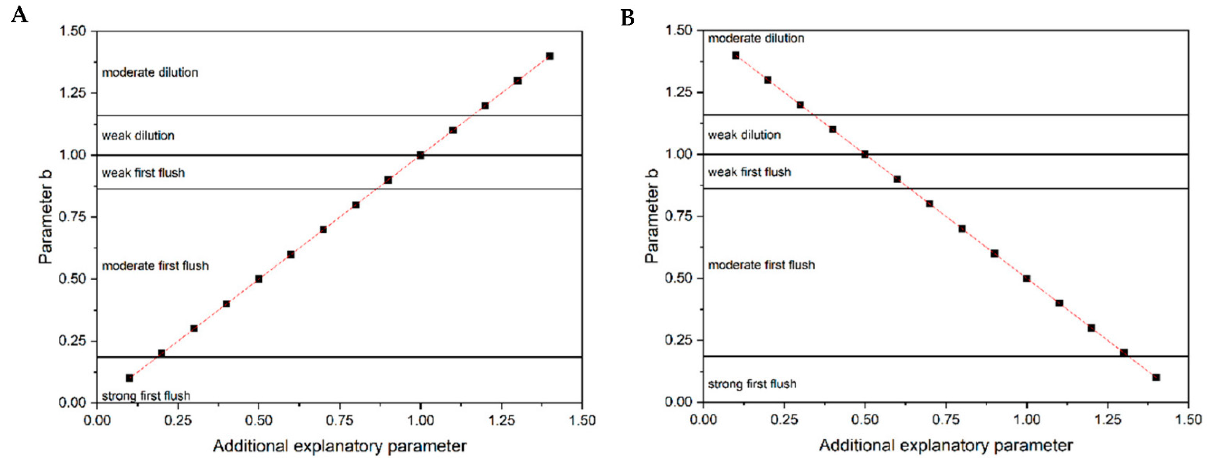
• Method 3 by Saget et al. [12]: differentiated classification of the first flush behavior into weak, moderate and strong using several thresholds

A detailed description of the methods used can be found in the Supplementary Data.

2.5. Additional Explanatory Parameters

As described in Section 1 the first flush effect can be affected by numerous parameters. In this study, 8 parameters were determined that may have an influence on the general occurrence, timing, and intensity of the first flush effect for all studied rainfall events. The following 8 parameters were calculated:

• Total rainfall depth [mm]: is defined as the total amount of precipitation that has fallen within a rainfall event. A rainfall event is finished when no precipitation has been recorded for 30 min.
• Average rainfall intensity [mm/h]: is defined as the average value of the recorded precipitation depth divided by the corresponding time interval of 5 min.
• Max 5 min intensity [mm/h]: is defined as the maximum recorded precipitation depth divided by the corresponding time interval of 5 min.
• Rainfall duration [min]: is defined as the time between the first and last recorded rainfall depth of a targeted rainfall event.
• Antecedent dry period [d]: is defined as the time prior a targeted rainfall event in which the total amount of rainfall depth is 1 mm.
• Average runoff depth [m]: is defined as the average recorded runoff inside the sewer system evoked by a targeted rainfall event.
• Total runoff volume [m³]: is defined as the total amount of water which passed the sampling site during a targeted rainfall event.
• Runoff peak [m]: is defined as the maximum recorded runoff depth.

2.6. Statistical Analysis

The calculated total pollutant load, pollutant-EMCs, described additional explanatory parameters and the calculated parameter b for the respective pollutant from all sampled rain events were used for correlation analysis using spearmen rank correlation. OriginPro 2021 (OriginLab Corporation, Northampton, MA, USA) including correlation plot app was used for statistical analysis. p ≤ 0.05, p ≤ 0.01 and p ≤ 0.001 were chosen as the levels of significance.

3. Results and Discussion

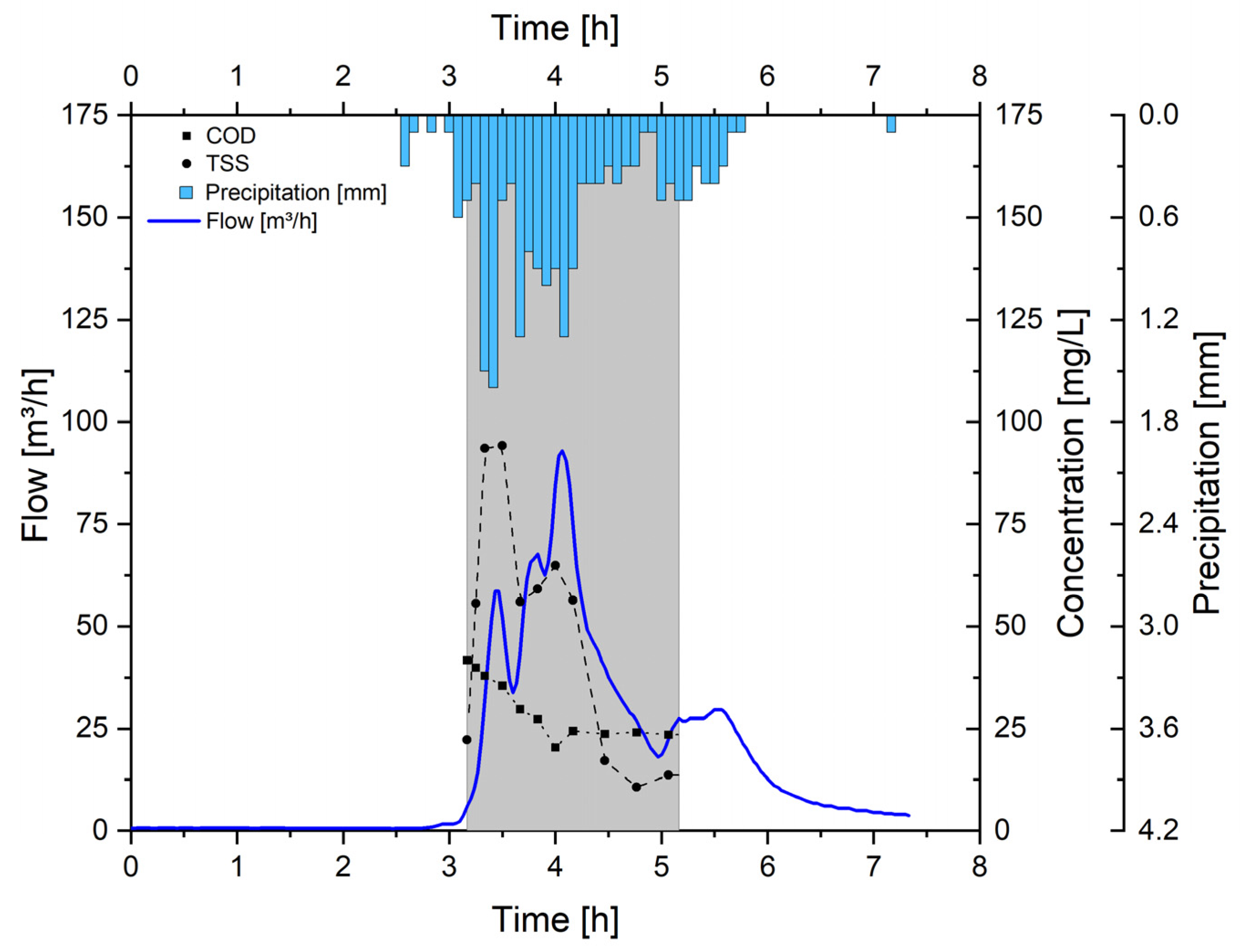
3.1. Temporal Variation in Runoff Pollution and Quantity

Table 3. Precipitation data of the 10 studied rainfall events.

Date	Total Rain [mm]	Mean Intensity [mm/h]	Max. Intensity [mm/h]	Rain Duration [min]	Antecedent Dry Period [d]
11 October 2020	1.60	2.13	4.80	90	1.07
18 October 2020	1.40	3.36	6.00	25	3.41
20 October 2020	3.20	1.60	3.60	126	0.04
23 October 2020	19.50	6.16	19.20	190	2.13
30 October 2020	6.50	1.44	4.80	430	0.70
12 January 2021	2.80	1.20	1.20	445	0.49
13 January 2021	2.00	4.00	6.00	25	1.03
18 January 2021	1.60	1.20	1.20	135	0.31
6 May 2021	2.70	2.16	4.80	110	3.75
11 May 2021	1.60	1.20	1.20	170	0.86

presents an overview of the rainfall characteristics during the studied rainfall events. The total precipitation ranges from 0.90 mm to 19.50 mm, while the mean rainfall intensity ranges from 1.20 mm/h to 6.16 mm/h. The highest rainfall intensity was measured on 23 October 2020 with 19.20 mm/h, which is 16 times higher than the lowest measured rainfall intensity. At this point it should be noted that lower intensities could not be determined due to the precipitation measurement system. The rainfall duration of the sampled rainfall events varies between 25 min and 1180 min, while the longest antecedent dry period was almost 18 days.

The routine water quality parameters studied provide important information about the general condition of stormwater.

Table 4. Stormwater quality parameters.

		This Study a	Ref. [20] b	Ref. [14] c	Ref. [21] d	Ref. [6] e
		Mean (Min–Max)	Average (Min-Max)	Mean ± Standard dev.	Median (Min-Max)	Mean (Max)
COD	mg/L	36.69 (9.97–72.20)	125 (48–230)	N/A	89 (14–320)	89 (354)
TSS	mg/L	29.13(0.04–238.34)	193 * (58–430)	140.7 ± 111.7	106 (11–430)	68 (352)
TP	mg P/L	1.13 (0.14–5.00)	1.52 (0.47–3.52)	0.29 ± 0.15	0.87 (0.30–3.52)	0.32 (0.92)
DP	mg P/L	0.70 (0.09–4.64)	N/A	0.09 ± 0.09	N/A	0.038 (0.15)
TKN	mg N/L	N/A	3.10 (1.5–5.94)	2.25 ± 1.41	2.8 (<2–16)	N/A
NO3	mg N/L	3.86 (0.79–11.06)	N/A	0.46 ± 0.35	N/A	N/A
NH4	mg N/L	0.92 (0.04–2.67)	N/A	0.45 ± 0.32 **	N/A	0.47 (1.1)

N/A Data not available; ^a Residential catchment, 5 ha, Braunschweig, Germany; ^b Dense urban area (commercial center, apartments, buildings), 2.30 km², Paris, France; ^c Dominated by roadways, 1.94 ha, Raleigh, NC, USA; ^d Three watersheds, residential, dense urban area and high-density urban area, Paris, France, including data from Zgheib et al. [20]; ^e Residential catchment, 16.2 ha, Berlin, Germany; * Suspended particulate matter (SPM); ** Data given as NO₃-N (mg/L).

presents results obtained for routine water quality parameters from this study and data adapted from other databases [6,16,20,21]. The data presented in Table 4 can be used for a general classification of the pollution potential based on measured concentrations. For the quality-based drainage concept, however, the general trend of pollution and flow and the derivation of pollution profiles in dependence of the individual rainfall characteristics are the relevant key factors and will be discussed in detail in the following. The concentration range and EMCs of all investigated pollutants are given in Figure S2 and Table S5, respectively (Supplementary Material).

In this study, the measured COD and TSS concentrations were low compared to existing measurement data. It is assumed that low COD concentrations could be related to the sampling period (October to May), since the majority of COD in stormwater is originated from surrounding vegetation or animals [22]. This assumption indicates additional seasonal stormwater quality dynamics. Typical sources of solids are tire wear, roadway wear, construction sites, atmospheric deposition, anthropogenic waste and soil particles transported by wind erosion [22,23]. The predominantly residential character of the watershed with low traffic intensity could result in low solid concentrations. In contrast, the mean nutrient concentrations are comparatively high indicating an intensive nutrient leaching during rain events or a contamination by infiltration of nutrient rich water. According to Yang and Lusk [24], atmospheric deposition, chemical fertilizers, organic materials, soil, and microbial sources (nitrification) are common sources for nitrogen and phosphorous in stormwater. At this point, a garden plot area in the immediate surrounding of the catchment area must be mentioned, as this area can operate as a source for fertilizer emissions into resulting in high nutrient concentrations in stormwater runoff. However, only the mean DP-concentrations reach similar concentrations compared to combined sewer overflows (CSO), while all other nutrient concentrations in this study do not reach concentration levels of nutrients measured in CSOs, e.g., obtained by Gasperi et al. [25]. A review of sources contributing to urban stormwater pollution is given by Müller et al. [17].

Figure 1 shows an exemplary rainfall event from October 2020 for potential pollutant dynamics during rainfall events. The runoff regime follows the rainfall patterns, with an increase in runoff immediately after beginning of the rainfall and a corresponding rapid decrease when the rainfall ends.

Runoff peaks are evident with maximum rainfall intensities. In this example, concentrations of COD decrease continuously throughout the sampling period regardless of flow. In contrast, TSS increases significantly at the beginning and is much more dependent on flow than COD as it progresses. Apparently, the first runoff water mobilizes solids deposited depending on flow. Furthermore, the concentration of TSS shows a rapid decrease with a simultaneous rapid decrease in flow as rainfall intensity and the discharge in the channel decreased consequently.

3.2. Results Method 1

Table 5. Method 1 results summary.

Pollutant	No. of Storms	Max. L′V′		Cumulative Flow @ Max. L′V′		Sampling Time [h] @ Max. L′V′
		Mean	Standard Dev.	Mean	Standard Dev.	Mean	Standard Dev.
COD	10	0.0583	0.0357	0.4692	0.2565	0.6542	0.3552
TSS	9	0.2282	0.1552	0.4577	0.2223	0.5521	0.3152
TP	10	0.0881	0.0610	0.4795	0.2148	0.6222	0.3707
DP	10	0.0510	0.0374	0.5572	0.3306	0.9021	0.6869
NO3	10	0.0477	0.0379	0.5135	0.2478	0.4905	0.2838
NH4	10	0.0845	0.0510	0.4837	0.1884	0.6033	0.3814

presents a summary of the results from method 1 analysis. The calculated maximum divergence between L′ and V′ for the investigated pollutants is between 0.0477 (NO₃⁻) and 0.2282 (TSS). Thus, a first flush behavior is observed on average for each pollutant. The higher the divergence value between L′ and V′ and the smaller the cumulative percentage of flow at maximum divergence, the more pronounced the first flush effect. Based on method 1, NO₃ appears to have the weakest first flush since the mean maximum divergence value is small. However, the mean cumulative percentage of flow at maximum divergence for NO₃ is slightly higher than the mean cumulative percentage of flow for NH₄. Conversely, TSS had the most prominent first flush effect with the largest obtained mean divergence value. Dissolved or partially dissolved pollutants have a maximum divergence value < 0.09 indicating no significant first flush effect for dissolved or partially dissolved pollutants compared to TSS. Furthermore, the mean maximum divergence for nutrient parameters occurs after a cumulative percentage of flow between 47.95% and 55.72%.

While the maximum divergence between L′ and V′ gives an indication of the intensity of the first flush effect, the cumulative flow and the absolute time after start of the sampling can be used to give a temporal and volumetric range of when a first flush occurs. Based on TSS as an indicator parameter, the mean cumulative discharges, calculated times and the described specific catchment, an exemplary scenario A for quality-based drainage can be defined as follows:

• The largest divergence between cumulative volume and cumulative load for TSS occurs on average after 45.77 % of the discharge volume or 0.55 h after a significant rise in water level inside the sewer or start of sampling, respectively (Table 5).
• If the stormwater is discharged separately to a centralized/decentralized treatment until the time of maximum divergence of the TSS, an average of 65.02% TSS load can be treated. For the investigated catchment area, this would also mean that an average of 1.41 m³/ha of stormwater and the specific pollution loads given in

  Table 6. Summary of specific volume and pollutant loads for scenario A.

  Cumulative TSS Load @ Max. L′V′	Specific Volume [m3/ha]	Specific Pollutant Load [g/ha]
  		COD	TSS	TP	DP	NO3	NH4
  Mean (Standard Dev.)
  0.6502 (0.1792)	1.41 (2.20)	46.37 (66.16)	71.69 (165.61)	2.27 (4.66)	1.29 (2.72)	3.89 (4.14)	0.84 (0.70)

  are discharged to treatment.

It should be noted that only average values were assumed for this consideration. The calculated standard deviations clearly show that a large volumetric and temporal range was determined for all investigated pollutants. Therefore, a specific characterization of stormwater pollution dynamics, and thus also a possible scenario for a quality-based drainage, is very complex. In addition, the investigation period (October–May) with no or very few heavy rainfall events must be considered.

3.3. Results Method 2

While method 1 does not provide any specific threshold to quantify the first flush effect, method 2 defines the first flush effect by the occurrence of a positive gap between the L′V′ curve and the bisector greater than 0.2 (Geiger [9]). The method 2 results are presented in

Table 7. Method 2 results summary.

Pollutant	No-of Storms	>0.2 Gap	%
COD	10	0	0
TP	10	0	0
DP	10	0	0
NO3	10	0	0
NH4	10	0	0
TSS	9	6	66.67

. Using method 2, only TSS exhibit a first flush effect in 66.67% of the storm events. Consequently, a further differentiation of the first flush intensity is necessary regarding a quality-based drainage.

3.4. Results Method 3

The results from method 3 provide further differentiation regarding the first flush intensity. The calculated mean b values for each pollutant are listed in

Table 8. Method 3 results summary.

Pollutant	Mean (Standard Dev.) b Coefficients
DP	1.077 (0.111)
TP	0.988 (0.136)
COD	0.977 (0.095)
NO3	0.966(0.120)
NH4	0.921 (0.141)
TSS	0.802 (0.233)

. Due to these investigations, the first flush intensity increases in the order DP < TP < COD < NO₃ < NH₄ < TSS. All pollutants except DP show an overall first flush nature, with mean b values less than 1. TSS shows the strongest and most frequent first flush behavior with mean b values of 0.802, while DP shows the weakest and least frequent first flush behavior with mean b values of 1.077 on average, indicating a dilution effect.

Saget et al. [12] suggested ranges of b values that correspond to the strength of the first flush effect (see Section 1.1.1). According to data analysis, DP has mean values (1.077) that fit into the weak dilution range, while TP, COD, NO₃ and NH₄ have mean b values (0.921–0.988) that fit into the weak first flush range. The mean b value for TSS is 0.802 and thus fits into the moderate first flush range. Hathaway et al. [14] determined mean b values of 0.75, 0.73, 0.76, 0.83, 0.97 and 1.13 for TSS, NH₃, TKN, TP, NO₃/NO₂ and DP, respectively. According to the results from Hathaway et al. [14], a first flush effect occurs on average for all parameters, except for DP. Thus, Hathaway et al. [16] determined similar b values for TSS, NO₃ and DP. Furthermore, Peng et al. [26] calculated b values for COD, NH₃-N, TP and suspended solids (SS) ranging 0.86–1.53, 0.77–1.47, 0.77–1.61 and 0.72–1.62, respectively, indicating the possible occurrence from moderate first flush to moderate dilution for all four pollutants. The calculated b values determined in this study were used as an indicator of the first flush effect in the correlation analysis (Section 3.6.) regarding a quality-based drainage.

3.5. Summary of Methods and Comparison of Pollutant First Flush Strength Regarding a Quality-Based Treatment

Considering all three analysis methodologies, TSS clearly shows the strongest first flush effect. The most intense first flush effect for TSS has been established by several previous studies [27,28,29,30]. Nitrogen species appeared to have stronger first flush effects than phosphorous, with orthophosphate showing the weakest first flush characteristics of all pollutants considered. Moreover, using method 3 for data analysis, DP even shows frequent dilution. Of all nitrogen species considered/measured, NH₄ appeared to have the strongest first flush effect, while NO₃ appeared to have the weakest. Nevertheless, both nitrogen species tended to have a stronger first flush behavior than COD. In contrast, Lee et al. [27] showed that the relative strength of the first flush effect for DP can be greater than the first flush effect of TKN and TP for a residential catchment, although the study shows no further differentiation between nitrogen species. Egemose et al. [30] published that in approximately 50% of the considered rainfall events, a larger part of SS and P was transported and discharged in the first part of the event, indicating a first flush tendency. The authors’ additional classification regarding dissolved or undissolved pollutants does not show a clear tendency. TSS, COD and TP showed a first flush effect as well as the dissolved nitrogen species, while a dilution effect was determined for DP.

Based on the results of this study, TSS is the most suitable indicator parameter for quality-based discharge, since trends with regard to the occurrence of first flush effects are more clearly recognizable than for any other pollutant investigated. A possible exemplary approach for quality-based discharge based on the TSS results has already been briefly explained in Section 3.2. Since building up knowledge about the behavior of TSS in sewer systems involves complex measurements and analytics, correlations between the first flush behavior of TSS (or other pollutants) with rainfall characteristics and antecedent dry periods could improve predictions about the occurrence and intensity of the first flush effect and thus contribute to an optimized quality-based drainage.

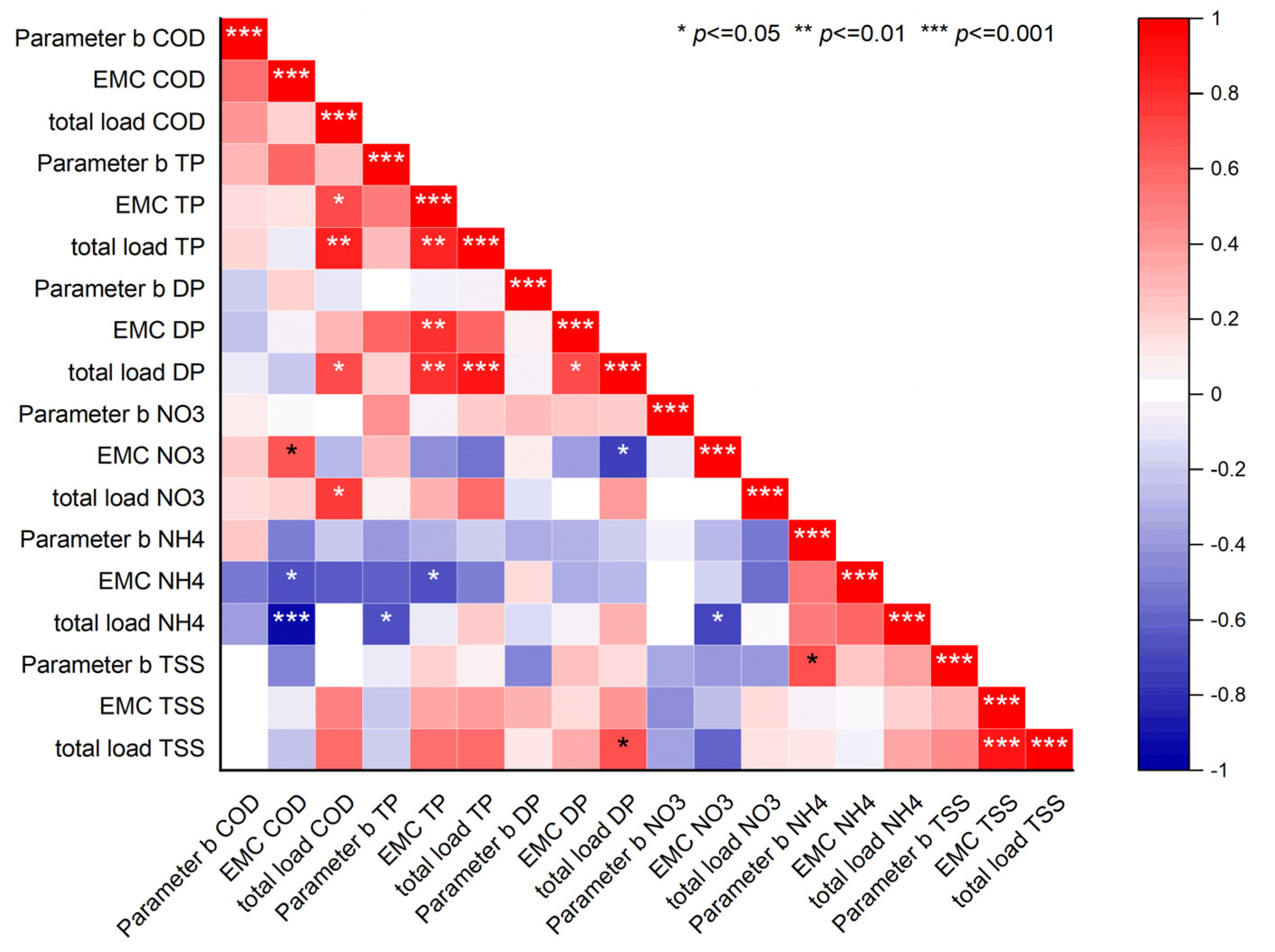
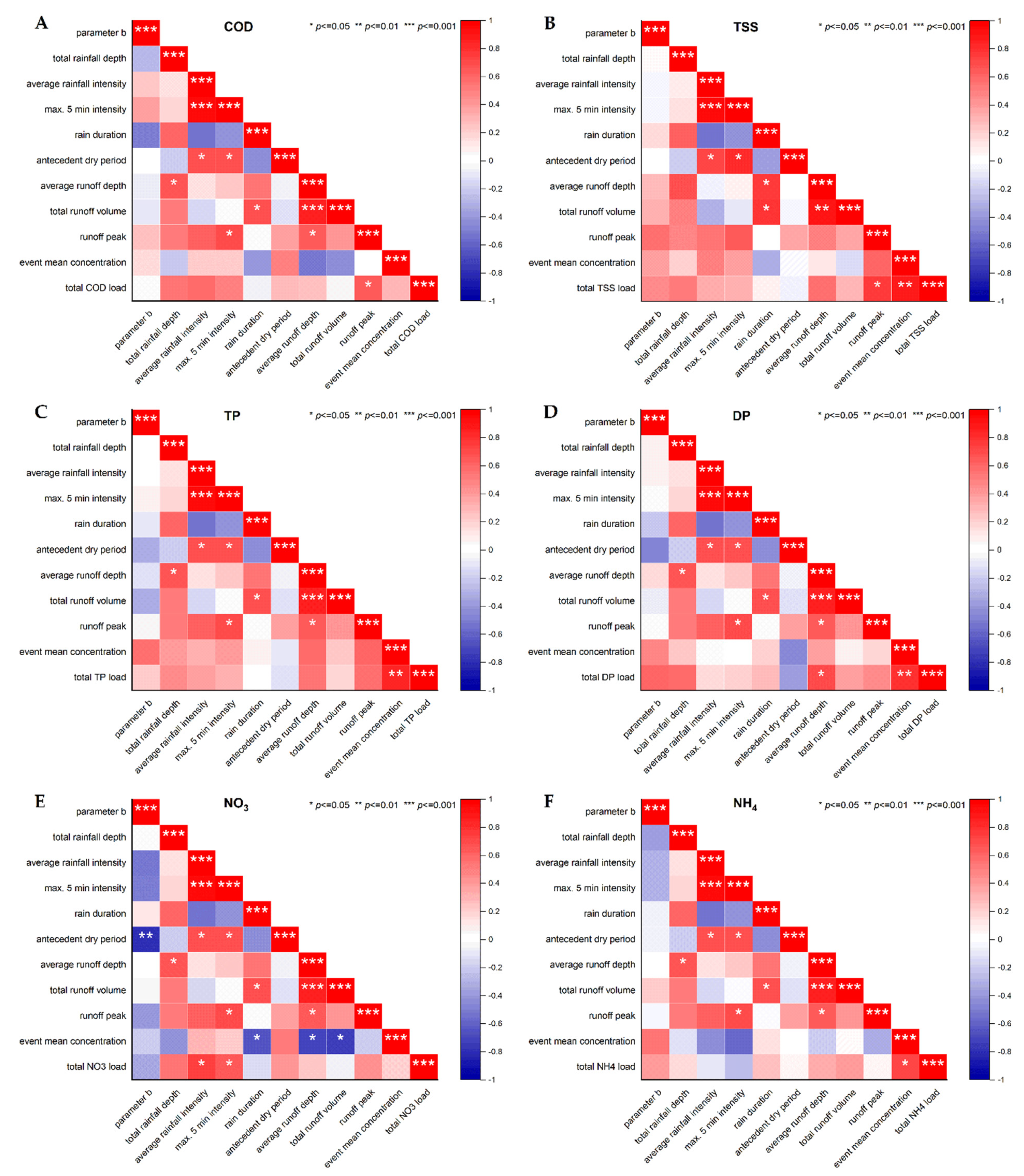
3.6. Correlation Analysis

To investigate possible correlations between the first flush effect and the given catchment and rainfall characteristics, spearman rank correlations for each pollutant were performed between the calculated parameter b and the described additional explanatory parameters with parameter b indicating the strength of the first flush. In addition, the EMCs and the total pollutant load were included. The level of significance was defined at p ≤ 0.05, additionally differentiated according to p ≤ 0.01 and p ≤ 0.001 indicted by *, ** or ***, respectively. The correlation patterns include red and blue squares. Red squares indicate a positive correlation. This means that a statistical increase in one value results in a statistical increase in the corresponding value. On the contrary, blue squares indicate a negative correlation. Here, a statistical increase in one value results in a statistical decrease in the corresponding value. Examples for both positive and negative correlation including the parameter b are given in Figure 2.

It should be noted, as shown in Figure 2A, a positive correlation of an explanatory parameter with the parameter b leads to a decreasing first flush behavior according to Table 1. In contrast, a negative correlation consequently leads to an increasing first flush behavior (see Figure 2B).

Figure 3 shows the results of the correlation analysis. The determined p-values for all cor-relation patterns are given in Figures S3 and S4, respectively (Supplementary Material).

The results of the correlation analysis for the investigated pollutants are very heterogeneous. For COD, no significant correlation between the parameter b and explanatory parameters were determined. While Park et al. [29] determined weak correlations for organic matter concentration during dry days, no significant correlation between the COD EMC and the antecedent dry period was calculated in this study. Costa et al. [31] observed an increasing COD EMC with an increasing average rainfall volume during flood events. In contrast, a decrease in COD EMC was determined in this study as the average runoff depth and peak flow in the channel increased.

No significant correlations were determined for the TSS parameter b. However, the explanatory parameters average runoff depth, total runoff volume and runoff peak tend to have a positive correlation (red squares) with parameter b, indicating that a dilution effect occurs for the TSS with increasing flow intensity inside the sewer. In contrast, the total TSS load has a significant positive correlation with the runoff peak. A positive correlation between the total TSS load and peak flow was also observed by Costa et al. [31] and Szelag et al. [32]. Furthermore, Egemose et al. [30], Costa et al. [31] and Szelag et al. [32] found a significant positive correlation between total TSS load and total discharged volume and Park et al. [29] showed a significant correlation between rainfall intensity and suspended solids (SS), while in this study no significant correlation between these parameters was determined. Egemose et al. [30] have also shown that the total TSS load depends additionally on the catchment size, the maximum sewer length and the intensity of previous rain events. In summary, the different results in these studies clearly show that further research for TSS variation and correlation is necessary in the investigated catchment.

No significant correlations were determined for the parameter TP and DP either. While the first flush effect for TP tends to correlate negatively (blue squares) with the parameters rain duration, antecedent dry period and total runoff volume, the analysis for DP tends to have a negative correlation only for rain duration and antecedent dry period. Egemose et al. [30] found a significant dependence of particulate P transport with catchment and rainfall characteristics which was not observed in this study. In addition, the previous rainfall event has an important influence on TP transport [30]. Besides the possibility of fertilizer emissions in the catchment area, Yang and Toor [33] hypothesize that in most residential catchments, natural sediments or soil materials are sources of DP. In addition to dissolution and desorption effects of these materials, DP may origin from dust particles and the degradation of organic material. These P sources could contribute to the TP and DP concentrations measured in this study. The influence of land use on phosphorous export in the catchment area is exemplary shown by Zhou [34] by determining a significant correlation between grass land and phosphorous export.

For both investigated nitrogen species, the tendency of a negative correlation of the additional explanatory parameters and parameter b for NO₃ and NH₄ was predominantly determined. Nevertheless, a significant correlation can only be shown between the parameter b and the antecedent dry period. In addition, a significant negative correlation between NO₃ EMC, rain duration, average runoff depth and total runoff volume were observed indicating a dilution effect for the EMC with increasing rain duration and the corresponding average and total runoff volume. In contrast, Costa et al. [31] showed that the greater the total volume, the greater the NO₃ concentrations and the greater the average rainfall volume, the higher the EMCs for NH₄ and NO₃. Yang and Toor [33] did not observe any relationship between measured variables and rainfall amount and intensity, although storm characteristics such as rainfall intensity and rainfall amount can influence N in stormwater runoff, due to atmospheric deposition. According to Yang and Toor [33], important sources of nitrogen in stormwater, besides atmospheric deposition, are dry deposition from vehicles, chemical fertilizers and soil. According to Taylor et al. [35], high variability of nitrogen during storm events is caused by variations in aerial deposition and rainfall quality, catchment soils and past and present catchment activities. Furthermore, Yang and Toor [33] attribute the variability to the switching of N sources over wet season such as runoff of fertilizer from turf, runoff of soil particles containing N and the depletion of N present in atmospheric deposition. All of the nitrogen sources mentioned could also be present in the investigated catchment area, which could explain the significant correlation between the first flush effect of NO₃ and the antecedent dry period due to a possible accumulation of nitrogen compounds in the catchment.

A classification of the parameters into dissolved and undissolved parameters does not give a clear tendency. For the pollutants that are present as solids or partially as solids (COD, TSS and TP), the parameter b for COD and TP tends to a negative correlation with most of the explanatory parameters. Thus, the strength of the first flush effect increases with increasing value of the respective explanatory parameter. However, only the described correlation between COD first flush strength and rain duration reaches a significant level. In contrast, the parameter b for TSS tends to show a positively correlated behavior with most of the explanatory parameters. It is noticeable that the rainfall characteristics (total rainfall depth, average rainfall intensity and max 5 min intensity) and the antecedent dry period are in a neutral range, although it seems reasonable to assume that the first flush for TSS should be more intensive due to intense rain or long antecedent dry periods. Perera et al. [36] investigated variables in terms of their importance in predicting first flush occurrence and ranked them with decreasing importance based on SS as follows: total rainfall depth, maximum 5 min rainfall intensity, rainfall duration, runoff depth, runoff peak, average rainfall intensity, antecedent dry period, effective impervious area, time of concentration and event mean concentration. The results of Perera et al. [36] support the poor correlation between TSS and antecedent dry period calculated in this study and show a comparatively low influence of the antecedent dry period on the first flush effect. The dissolved parameters also show a heterogenous behavior. While the parameter b for the nitrogen species tends to correlate negatively with most of the explanatory parameters, the parameter b for dissolved phosphorus tends to show a negative correlation only with the rain duration and antecedent dry period.

While the correlation analysis for the individual pollutants with explanatory parameters mainly gives a heterogenous picture, a correlation analysis of the different pollutants with each other could provide additional information with regard to the first flush behavior. The level of significance was defined at p ≤ 0.05, p ≤ 0.01 and p ≤ 0.001 indicated by *, ** or ***, respectively. Figure 4 shows the results of the correlation analysis between parameter b, pollutant EMCs and total pollutant loads.

The correlation pattern for the investigated pollutants (Figure 4) shows a significant negative correlation between COD EMC, NH₄ EMC and total NH₄ load, respectively, while a significant positive correlation between COD EMC and NO₃ EMC was calculated. Furthermore, the total NO₃ load increase with increasing COD EMC. For NO₃ and NH₄, Costa et al. [31] and Zhao et al. [37] also determined a positive correlation with EMC COD. Consequently, the results for NO₃ are in line with results from previous studies, indicating that COD an NO₃ originate from the same or very similar source. However, for the correlation between COD and NH₄, contradictory results were obtained in this study. Furthermore, a significant positive correlation between TP EMC, DP EMC and total DP load as well as a significant correlation between total TP load and total DP load were obtained indicating that a considerable part of TP is dissolved as DP, which is similar to results obtained by Egemose et al. [30]. The obtained positive correlation between total DP load and total TSS load indicating that a fraction of DP might be either particulate bound or loosely adsorbed P [30]. Only the parameter b for TSS correlates positively with the parameter b for NH₄, which suggests that with decreasing or increasing first flush behavior of TSS, the first flush of NH₄ shows a corresponding behavior.

3.7. Summary of Correlation Analysis Regarding a Quality-Based Treatment

The correlation analysis clearly shows that further research is required in order to obtain a more specific relationships between first flush intensity, pollutant properties and the boundary conditions. It also shows that in addition to explanatory parameters, individual pollutant properties and sources must be considered with regard to quality-based discharge, which makes the control of quality-based discharge more complicated. For this purpose, in-depth and frequent measurements of indicator parameters, such as TSS, and the respective correlation analysis could be used for controlling a quality-based discharge. As a result, TSS and other pollutants can be specifically eliminated, e.g., by partial flow treatment.

4. Conclusions

The stormwater quality determined in this study does not differ particularly from stormwater qualities of previous studies, as the studied sub-catchment does not represent a focal point of pollution for the receiving water body with regard to the investigated pollutants. Based on method 3, the ranking of the first flush strength among the pollutants was TSS > NH₄ > NO₃ > COD > TP > DP. Nitrogen species show a stronger first flush behavior than phosphorous, with DP showing an average dilution effect. Both aspects were also determined by Hathaway et al. [14]. It should be noted that dissolved nitrogen species can have a moderate first flush behavior, highlighting the necessity of an adequate treatment as standard treatment technologies for stormwater are mainly based on filtration and not nutrient removal.

Quality-based management of stormwater can allocate all stormwater runoff classified as highly polluted to a centralized treatment. However, the implementation of discharge differentiation requires knowledge about the first flush behavior of one or more target pollutants. The statistical analysis methods to classify the first flush effect used in this study show a wide volumetric and temporal range for all investigated pollutants.

Due to the uncertainties explained, the correlation of the first flush behavior with additionally explanatory parameters such as total rainfall depth, average rainfall intensity, max 5 min intensity, rain duration, antecedent dry period, average runoff depth, total runoff volume and runoff peak is essential for the prediction of a first flush behavior. The additional explanatory parameters investigated in this study showed a mainly heterogenous correlation. Both, when considering the pollutants individually and among themselves, possibly due to an insufficient quantity of data. While the parameter b representing the slope of the linear regression equation tends to show a negative correlation with the pollutants that are present partially as solids, the parameter b for TSS tends to show a positive correlation with most of the explanatory parameters. In addition, dissolved nitrogen species tend to correlate negatively with most of the explanatory parameters, while the parameter b for DP tends to show a negative correlation only with the antecedent dry period. In summary, general pollution trends are identifiable and can thus be used for the dynamization of runoff pollution and quantity representing key parameters within a quality-based drainage concept. Knowledge about the temporal variation of urban runoff pollution can support short term decision making, e.g., as an input parameter for the regulation of a quality-based sewage switch. However, further research is needed to identify additional explanatory parameters with significant influence on pollution and runoff trends.

The general principle of the first flush, as well as the described methods for characterizing its strength, are increasingly important for stormwater management concepts. However, attempts to identify, classify and describe the first flush effect often result in considerable uncertainties, due to an extraordinary variety of influencing factors. The variation of pollutant sources, catchment characteristics, rainfall characteristics, physical and chemical properties of the pollutant show the necessity of further stormwater quality measurements and multivariable statistical methods to identify significant influences on the prediction of the first flush occurrence and intensity. In addition, future research should consider a land use characterization regarding the potential pollution from different surfaces to enhance the assessment of catchment characteristics. The results of this study explicitly focus on quality-based drainage to enhance climate-adapted transformation of existing urban neighborhoods. This concept was developed for dense urban structures and is directed towards the development of neighborhood-oriented water drainage and supply. The infrastructural settings of rural areas differ significantly from this, so that neither the concept nor the results of this study are transferable to rural areas. In the urban context, supplementary scenario analysis on the influence of rainfall characteristics on the behavior of emerging pollutants such as biocides could improve quality-based drainage management.

References

1. Lundy, L.; Ellis, J.B.; Revitt, D.M. Risk prioritisation of stormwater pollutant sources. Water Res. 2012, 46, 6589–6600. [Google Scholar] [CrossRef] [PubMed]
2. Sillanpää, N.; Koivusalo, H. Stormwater quality during residential construction activities: Influential variables. Hydrol. Process. 2015, 29, 4238–4251. [Google Scholar] [CrossRef]
3. Kozak, C.; Fernandes, C.V.S.; Braga, S.M.; do Prado, L.L.; Froehner, S.; Hilgert, S. Water quality dynamic during rainfall episodes: Integrated approach to assess diffuse pollution using automatic sampling. Environ. Monit. Assess. 2019, 191, 402. [Google Scholar] [CrossRef] [PubMed]
4. Ellis, J.B.; Mitchell, G. Urban diffuse pollution: Key data information approaches for the Water Framework Directive. Water Environ. J. 2006, 20, 19–26. [Google Scholar] [CrossRef]
5. Song, H.; Qin, T.; Wang, J.; Wong, T.H.F. Characteristics of Stormwater Quality in Singapore Catchments in 9 Different Types of Land Use. Water 2019, 11, 1089. [Google Scholar] [CrossRef] [Green Version]
6. Wicke, D.; Matzinger, A.; Sonnenberg, H.; Caradot, N.; Schubert, R.-L.; Dick, R.; Heinzmann, B.; Dünnbier, U.; von Seggern, D.; Rouault, P. Micropollutants in Urban Stormwater Runoff of Different Land Uses. Water 2021, 13, 1312. [Google Scholar] [CrossRef]
7. Köster, S.; Beier, M.; Kabisch, N.-K. Quality-based drainage of urban rainwater: Potential analysis for the catchment of Hildesheim, GER; Oral presentation and abstract. In Proceedings of the 15th International Conference on Urban Drainage, Melbourne, Australia, 25–28 October 2021. [Google Scholar]
8. Helsel, D.R.; Kim, J.I.; Grizzard, T.J.; Randall, C.W.; Hoehn, R.C. Land use influences on metals in storm drainage. J. Water Pollut. Control. Fed. 1979, 51, 709–717. [Google Scholar]
9. Geiger, F.W. Characteristics of combined sewer runoff. In Proceedings of the 3rd International Conference on Urban Storm Drainage; Balmer, P., Malmquist, P.-A., Sjöberg, A., Eds.; Chalmers University of Technology: Göteborg, Sweden, 1984; pp. 851–860. [Google Scholar]
10. Geiger, F.W. Flushing effects in combined sewer systems. In Proceedings of the 4th International Conference on Urban Storm Drainage; Gujer, W., Krejci, V., Eds.; École polytechnique fédérale de Lausanne: Lausanne, Switzerland, 1987; pp. 40–46. [Google Scholar]
11. Gupta, K.; Saul, A.J. Specific relationships for the first flush load in combined sewer flows. Water Res. 1996, 30, 1244–1252. [Google Scholar] [CrossRef]
12. Saget, A.; Chebbo, G.; Bertrand-Krajewski, J.-L. The first flush in sewer systems. Water Sci. Technol. 1996, 33, 101–108. [Google Scholar] [CrossRef]
13. Bach, P.M.; McCarthy, D.T.; Deletic, A. Redefining the stormwater first flush phenomenon. Water Res. 2010, 44, 2487–2498. [Google Scholar] [CrossRef]
14. Hathaway, J.M.; Tucker, R.S.; Spooner, J.M.; Hunt, W.F. A Traditional Analysis of the First Flush Effect for Nutrients in Stormwater Runoff from Two Small Urban Catchments. Water Air Soil Pollut. 2012, 223, 5903–5915. [Google Scholar] [CrossRef]
15. Deletic, A. The first flush load of urban surface runoff. Water Res. 1998, 32, 2462–2470. [Google Scholar] [CrossRef]
16. Bertrand-Krajewski, J.-L.; Chebbo, G.; Saget, A. Distribution of pollutant mass vs volume in stormwater discharges and the first flush phenomenon. Water Res. 1998, 32, 2341–2356. [Google Scholar] [CrossRef]
17. Müller, A.; Österlund, H.; Marsalek, J.; Viklander, M. The pollution conveyed by urban runoff: A review of sources. Sci. Total Environ. 2020, 709, 136125. [Google Scholar] [CrossRef] [PubMed]
18. DWD. Climate Data Center (CDC): Annual Mean of Station Observations of Air Temperature at 2 m above Ground in °C for Germany, Station-ID 662 Braunschweig, Germany, 1990–2020, version v21.3. Available online: https://cdc.dwd.de/portal/202107291811/mapview (accessed on 10 December 2021).
19. DWD. Climate Data Center (CDC): Annual Station Observations of Precipitation in mm for Germany, Station ID 662 Braunschweig, Germany, 1990–2020, version v21.3. Available online: https://cdc.dwd.de/portal/202107291811/view1 (accessed on 10 December 2021).
20. Zgheib, S.; Moilleron, R.; Saad, M.; Chebbo, G. Partition of pollution between dissolved and particulate phases: What about emerging substances in urban stormwater catchments? Water Res. 2011, 45, 913–925. [Google Scholar] [CrossRef]
21. Zgheib, S.; Moilleron, R.; Chebbo, G. Priority pollutants in urban stormwater: Part 1—Case of separate storm sewers. Water Res. 2012, 46, 6683–6692. [Google Scholar] [CrossRef]
22. Barbosa, A.E.; Fernandes, J.N.; David, L.M. Key issues for sustainable urban stormwater management. Water Res. 2012, 46, 6787–6798. [Google Scholar] [CrossRef]
23. Aryal, R.; Vigneswaran, S.; Kandasamy, J.; Naidu, R. Urban stormwater quality and treatment. Korean J. Chem. Eng. 2010, 27, 1343–1359. [Google Scholar] [CrossRef]
24. Yang, Y.-Y.; Lusk, M.G. Nutrients in Urban Stormwater Runoff: Current State of the Science and Potential Mitigation Options. Curr. Pollut. Rep. 2018, 4, 112–127. [Google Scholar] [CrossRef]
25. Gasperi, J.; Zgheib, S.; Cladière, M.; Rocher, V.; Moilleron, R.; Chebbo, G. Priority pollutants in urban stormwater: Part 2—Case of combined sewers. Water Res. 2012, 46, 6693–6703. [Google Scholar] [CrossRef] [Green Version]
26. Peng, H.-Q.; Liu, Y.; Wang, H.-W.; Gao, X.-L.; Ma, L.-M. Event mean concentration and first flush effect from different drainage systems and functional areas during storms. Environ. Sci. Pollut. Res. Int. 2016, 23, 5390–5398. [Google Scholar] [CrossRef] [PubMed]
27. Lee, J.H.; Bang, K.W.; Ketchum, L.H.; Choe, J.S.; Yu, M.J. First flush analysis of urban storm runoff. Sci. Total Environ. 2002, 293, 163–175. [Google Scholar] [CrossRef]
28. Hathaway, J.M.; Hunt, W.F. Evaluation of First Flush for Indicator Bacteria and Total Suspended Solids in Urban Stormwater Runoff. Water Air Soil Pollut. 2011, 217, 135–147. [Google Scholar] [CrossRef]
29. Park, M.; Choi, Y.S.; Shin, H.J.; Song, I.; Yoon, C.G.; Choi, J.D.; Yu, S.J. A Comparison Study of Runoff Characteristics of Non-Point Source Pollution from Three Watersheds in South Korea. Water 2019, 11, 966. [Google Scholar] [CrossRef] [Green Version]
30. Egemose, S.; Petersen, A.B.; Sønderup, M.J.; Flindt, M.R. First Flush Characteristics in Separate Sewer Stormwater and Implications for Treatment. Sustainability 2020, 12, 5063. [Google Scholar] [CrossRef]
31. Costa, M.E.L.; Carvalho, D.J.; Koide, S. Assessment of Pollutants from Diffuse Pollution through the Correlation between Rainfall and Runoff Characteristics Using EMC and First Flush Analysis. Water 2021, 13, 2552. [Google Scholar] [CrossRef]
32. Szeląg, B.; Górski, J.; Bąk, Ł.; Górska, K. The Impact of Precipitation Characteristics on the Washout of Pollutants Based on the Example of an Urban Catchment in Kielce. Water 2021, 13, 3187. [Google Scholar] [CrossRef]
33. Yang, Y.-Y.; Toor, G.S. Sources and mechanisms of nitrate and orthophosphate transport in urban stormwater runoff from residential catchments. Water Res. 2017, 112, 176–184. [Google Scholar] [CrossRef]
34. Zhou, L. Correlations of Stormwater Runoff and Quality: Urban Pavement and Property Value by Land Use at the Parcel Level in a Small Sized American City. Water 2019, 11, 2369. [Google Scholar] [CrossRef] [Green Version]
35. Taylor, G.D.; Fletcher, T.D.; Wong, T.H.F.; Breen, P.F.; Duncan, H.P. Nitrogen composition in urban runoff—Implications for stormwater management. Water Res. 2005, 39, 1982–1989. [Google Scholar] [CrossRef]
36. Perera, T.; McGree, J.; Egodawatta, P.; Jinadasa, K.B.S.N.; Goonetilleke, A. Taxonomy of influential factors for predicting pollutant first flush in urban stormwater runoff. Water Res. 2019, 166, 115075. [Google Scholar] [CrossRef] [PubMed]
37. Zhao, L.; Liu, X.; Wang, P.; Hua, Z.; Zhang, Y.; Xue, H. N, P, and COD conveyed by urban runoff: A comparative research between a city and a town in the Taihu Basin, China. Environ. Sci. Pollut. Res. Int. 2021, 28, 56686–56695. [Google Scholar] [CrossRef] [PubMed]
Figure 1. Variation in pollution dynamics during a rainfall event showing the runoff flow (1st y-axis), pollutant concentration (2nd y-axis, parameters COD (■) and TSS (●)) and precipitation data (3rd y-axis) over time.
Water 14 00418 g001
Figure 2. Examples for a positive (A) and negative (B) correlation including parameter b.
Water 14 00418 g002
Figure 3. Correlation pattern for investigated pollutants COD (A), TSS (B), total P (C), dissolved P (D), NO3 (E) and NH4 (F) with level of significance * = p ≤ 0.05, ** = p ≤ 0.01 and *** = p ≤ 0.001. Red squares indicating a positive, blue squares indicating a negative correlation coefficient.
Water 14 00418 g003
Figure 4. Correlation pattern for investigated pollutants with parameter b, pollutant EMCs and total pollutant loads with level of significance * = p ≤ 0.05, ** = p ≤ 0.01 and *** = p ≤ 0.001. Red squares indicating a positive, blue squares indicating a negative correlation coefficient, respectively.
Water 14 00418 g004