An Urban Water Pollution Model for Wuhu City

Abstract

An in-depth study of the temporal and spatial distribution of pollution loads can assist in the development of water pollution remediation. The research scope of this paper was the highly developed Wuhu City located south of the Yangtze River. Chemical oxygen demand (COD), NH₃-H, and total phosphorus (TP) were chosen as the pollutant research objects of this study. Then, by combining the natural and social conditions within the scope of the study, a balanced system of pollution load generation and migration was described. A pollution load model of Wuhu City based on Load Calculator, MIKE 11, and ArcGIS was established. The results indicate that, in terms of the time distribution, the changes in the influx of the different pollutants were consistent. In terms of the spatial distribution, the major contributions to the annual pollution load were domestic pollution, urban surface runoff pollution, and poultry breeding pollution. The major contributors to the annual pollution load into the river were domestic pollution, urban surface runoff pollution, and sewage plant tail water pollution. This analysis provides references for the comprehensive management of local water environments.

1. Introduction

Aquatic environmental pollution and secondary disasters have become global environmental issues. Based on the causes, aquatic environmental pollution can be divided into two categories: point source pollution and non-point source (NPS) pollution [1]. Compared with point source pollution, NPS pollution is characterized by an extensive distribution, complicated causes, and control difficulties. NPS pollution has become the primary pollution source in aquatic environments. In China, the quality of the aquatic environment has declined sharply due to the increasing pollution loads (such as ammonia, total phosphorus (TP), and chemical oxygen demand (COD)) from NPS pollution. Therefore, a comprehensive understanding of the temporal and spatial distribution characteristics of the pollution load would improve regional aquatic environmental treatment.

Since the 1970s, numerous scholars have investigated pollution load issues using quantitative data and mathematical models. Sator [2] conducted a study on the pollution characteristics of surface sediments, demonstrating that the pollutant content significantly correlated with particle size. Collins and Ridgway [3] studied the runoff characteristics of different pollutants in urban surface runoff, indicating that biochemical oxygen demand (BOD), suspended sediment (SS), NH₃-N, TP, and other common pollutants had good correlations.

Model simulation is regarded as the most effective and direct method to estimate NPS pollutants [4]. There are many models to quantify the effect of temporal–spatial changes on NPS pollution. Whipple et al. [5] proposed a cumulative scoring model that described the laws governing surface runoff and sewage discharge. Researchers in the United States successively introduced the storm water management model (SWMM) and the storage treatment overflow runoff model (STORM) to simulate urban runoff pollution [6,7]. In 2019, Korean scholars [8] selected three basins with different land cover characteristics for NPS pollution monitoring. Their results showed that COD correlated strongly with SS and TOC in all watersheds. It was challenging to explain the NPS pollution runoff based on specific characteristics, such as land cover. Anna Malagó et al. [9] used the Soil and Water Assessment Tool (SWAT) based on grid cells of 5 min of resolution to assess the processes involved in nitrate load generation and transport into aquifers and rivers. It provides basin management strategies for nitrate reduction in the Po River basin (Italy).

The study of NPS pollution in China began with an investigation of lake eutrophication in the early 1980s [10]. Zhu et al. [11] established an empirical statistical model to analyze the water quality data of receiving waters. The model obtained the output of NPS pollution from a catchment. Elsewhere, a method that quantitatively divides the rainfall intensity to calculate the urban runoff pollution load was proposed [12]. The integration of water quality models [13], 3S technology [14], and basin water quality management has become a new direction for pollution load research in the new century. Using BOD₅ as an example, another study [15] calculated the pollution load of Shenzhen Bay based on the total maximum daily loads (TMDLs) to propose water quality improvement routes. Long et al. [16] used the annual output coefficient and the river inflow coefficient to create a temporal and spatial distribution model of NPS pollution load in the Three Gorges Reservoir area. Moreover, Chen et al. [17] used a mass balance approach to quantify the sources of N discharge and analyzed the effect of land-use composition on riverine N export, taking Zhejiang Province, China, as a case study. This research suggests that human activities dominantly influence riverine nitrogen export, while land use only mediates it. Jiang et al. [18] built a coastal water pollution load model using system dynamics coupled with water pollution load and the “concentration loss” model. In 2019, Zhang et al. [19] modified the runoff module of SWAT to study the distribution properties and NPS control in the Binjiang watershed, southern China. The northeast sub-basins in lower terrain, used mainly for agricultural applications, were the critical source areas (CSAs). A year later, Ren [20] used multiple remote sensing images to predict the total pollution load of drinking water sources. The SWAT model studied the NPS pollution in the Miyun Reservoir Watershed. The results show that the total nitrogen load was much higher than that of the total phosphorus.

The pollution loads resulting from various land-use types showed significant spatial differences: agricultural land (followed by grassland) had the highest TN and TP loads per unit area [21]. Xie et al. [22] analyzed the spatial distribution characteristics of Beijing’s pollution load using inventory, equivalent standard load, cluster, and ArcGIS analyses. In 2021, Zhao [23] used the InfoWorks ICM model to obtain basic urban information and urban NPS pollution emission parameters. They also calculated the urban NPS pollution load of Kunming. Moreover, using a GIS-based empirical model, Liu et al. [24] identified the output and spatial characteristics of the pollution emissions in Dongguan City in South China. The method was effective for systematically studying the characteristics of runoff pollution in some highly urbanized regions. Another report [25] proposed an integrated approach to estimate agricultural and urban NPS pollution in an urban agglomeration watershed. It involves combining SWAT, the event mean concentration (EMC) method, and the Storm Water Management Model (SWMM) to guide water environment management plans considering agricultural and urban NPS pollution in an urban catchment.

According to the open literature, the models for calculating the NPS pollution load in watersheds may be divided into export coefficient models, empirical-based models, and physically based models [26]. The export coefficient model is usually used to evaluate and predict the effects of management policies annually. It calculates the pollution load as TN and TP but ignores the movement and transformation of pollutants in the water cycle. The empirical-based model is mainly based on the statistical analysis of rainfall, hydrology, and water quality monitoring data. These two models also ignore pollutants’ migration and transformation.

In contrast, physically based models may aid in simulating pollutant behavior in watersheds. These models combine detailed mathematical descriptions of soil erosion, rainfall runoff, pollutant transport, and transformation, and they provide a temporal and spatial view of water pollution. Therefore, these models have been widely used globally with satisfactory results. Popular models for NPS calculation include ANSWERS, AnnAGNPS, HSPF, SWAT, SWMM, etc. (

Table 1. Comparison of five hydrological models.

Model	Module	Time Step	Enabled Application
ANSWERS	Runoff/infiltration, sediment, evaporation	One-minute/daily time step	Suitable for medium-sized agricultural watersheds; designed for ungauged watersheds; evaluates the effect of best management practices on reducing soil erosion and nutrients; capable of simulating pollutant transport and transformation [4].
AnnAGNPS	Hydrology, erosion, pollutant transportation, chemicals	Daily time step	Suitable for agriculture watersheds; efficient for annual and monthly simulation; efficient for large-scale simulation of runoff, soil erosion, and nutrient runoff; evaluates the effect of conservation practices [27].
HSPF	Hydrology, erosion, pollutants	One-minute/daily time step	Suitable for agricultural and urban watersheds in a long time series; accesses the effect of the point or NPS pollution treatment and land-use change [28].
SWAT	Hydrology, meteorology, sediment, soil, crop growth, pollutants and agricultural chemicals	Daily time step	Much suitable for large agriculture watersheds; excellent for calculating total maximum daily loads; evaluates the effect of best management practices on reducing sediment and nutrient runoffs [29].

)

The Danish Hydraulic Institute (DHI) developed a pollution load assessment tool, the Load Calculator, in November 2018. This integrated tool is convenient and has a relative universality; it combines hydrology with pollutant migration and transformation processes. The different modules in this tool involve the above three models, and they have their advantages. This tool estimates various point sources and NPS pollution loads, and it evaluates the water quality of river basins and urban water bodies [30]. Currently, the Load Calculator is used in the preliminary planning of aquatic environmental comprehensive management strategies [31]. Few studies have used this tool to assess pollution’s temporal and spatial distribution.

Wuhu City, a vital transit city on the Yangtze River, was selected as the research object in this study. The “Yangtze River Conservation” and “Yangtze River Economic Belt” strategies have demanded relatively high standards for the water environment of this city in recent years. Thus, the water environment protection of Wuhu City is strategically significant. A comprehensive investigation of the temporal and spatial distribution of the pollution load of Wuhu can help guide the aquatic environmental management of Wuhu City. Meanwhile, this study’s research methods and conclusions also have reference significance for other cities along the Yangtze River, promoting the conservation of the Yangtze River and the healthy development of the Yangtze River Economic Belt.

Based on this, the objectives of this study were to establish a pollution load model of Wuhu City using the Load Calculator and to discuss the distribution characteristics of the regional pollution load.

2. Materials and Methods

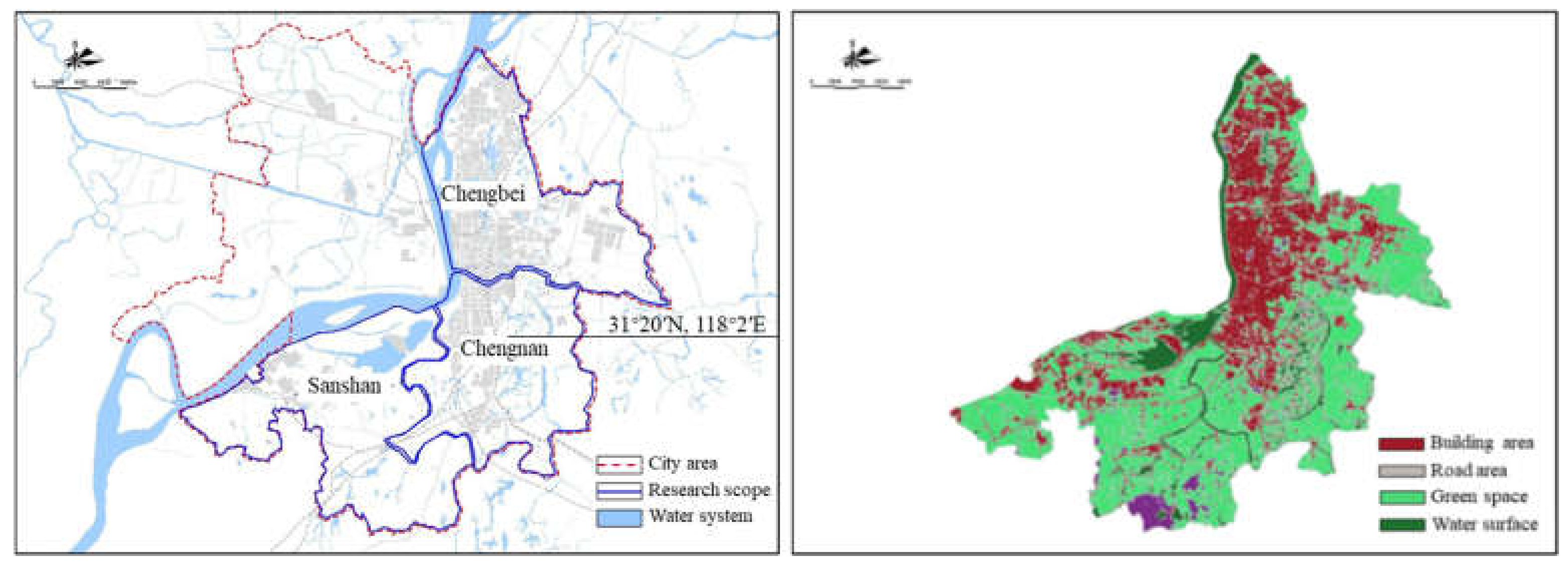
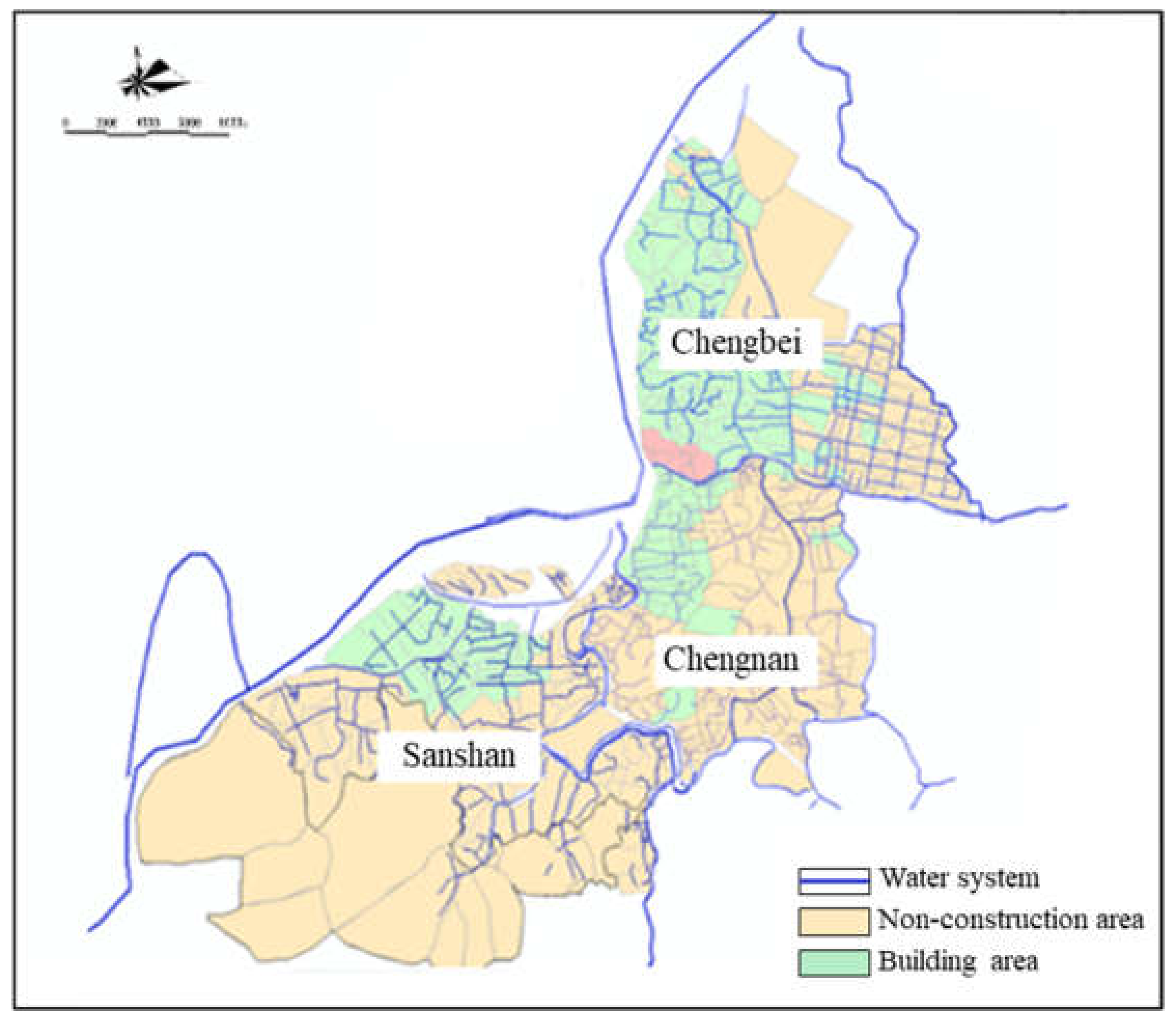
2.1. Study Area

Wuhu City is located in the southeast of Anhui Province and belongs to the lower reaches of the Yangtze River. The geographic coordinates of the center are 31°20′ N, 118°2′ E, and the total area of the primary urban area is 6026 km². It is primarily composed of floodplains and terraces. The overall topography is higher in the southwest and lower in the northeast, and the plain elevation is generally between 6.0 m and 12.0 m (Wusong elevation). The multi-year average (1956–2010 series) precipitation is 1227 mm, and the annual average rainfall in the area south of the Yangtze River is 1271 mm. The rainfall is unevenly distributed during the year, but the annual rainfall is primarily concentrated during the flood season from May to September, and this time accounts for greater than 60% of the annual rainfall. The inter-annual rainfall variation is three times greater between the wet and dry years.

Wuhu City belongs to the Yangtze River basin, which contains more than 50 rivers and 20 lakes. The total length of the rivers can reach up to 869 km, and the total water area is approximately 797 km². The primary rivers in the territory include the Yangtze River, Qingyi River, Shuiyang River, Zhang River, Xi River, and Yuxi River. The primary lakes include Zhusi Lake, Heisha Lake, Longwo Lake, Nantang Lake, Kui Lake, and Fengming Lake.

The aquatic environmental condition in Wuhu City has a significant effect on the lower reaches of the Yangtze River. This study scope was divided into three areas, namely, the Chengbei area, the Chengnan area, and the Sanshan area, and the study considered the drainage patterns and administrative divisions. Refer to

Table 2. Statistics of the study area.

Surface Type	Building Area (km2)	Road Area (km2)	Green Space (km2)	Water Surface (km2)	Other Areas (km2)	Total (km2)
Chengbei	116.49	1.10	11.06	7.24	108.28	243
Chengnan	25.52	0.27	176.59	0.08	7.24	210
Sanshan	16.23	0.26	194.34	0.76	22.24	234

for the statistics of the study area, and Figure 1 for the general boundary divisions and land use in each area.

To simulate the changes in the hydrodynamics and the migration of pollutants within the scope of the study, a corresponding model was established in this study. By utilizing DHI series software, in combination with the hydrodynamic model, the water quality model, and the pollution load model, the water pollution load in the study area was analyzed and simulated. The construction schematic of the model is shown in Figure 2. The data processed in the hydrodynamic model and pollution load model in the early stage included the statistical divisions, the catchment area distribution, the river network distribution, and land-use types.

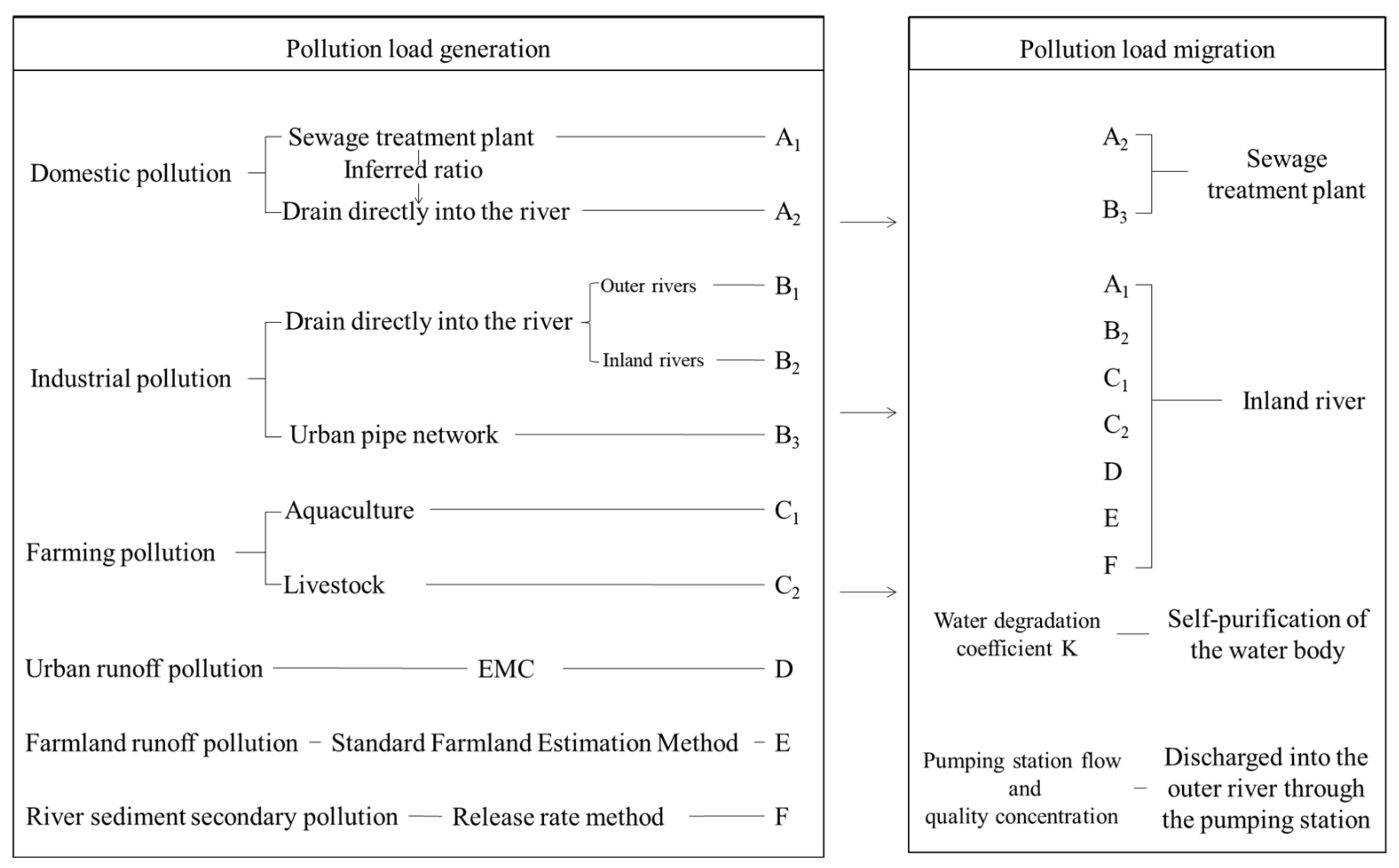
2.2. Pollution Load Generation and Migration Balance

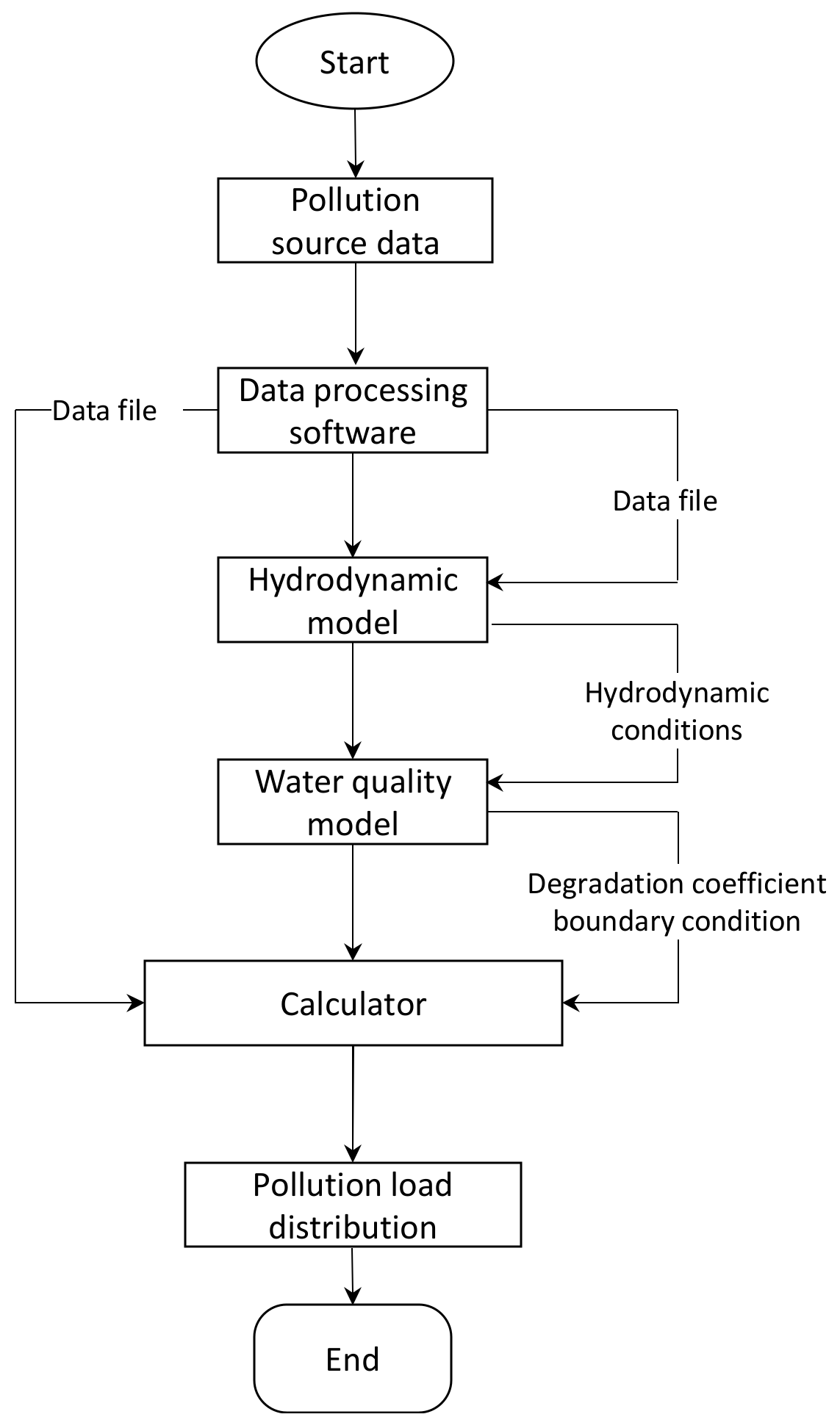
Using an investigation and analysis of the study area, the water pollution load generation and migration balance system was described. The pollution load primarily originated from six major sources, which included domestic pollution, industrial pollution, farming pollution, farmland runoff pollution, urban runoff pollution, and river sediment secondary pollution. In addition, the pollution load traveled through four migration routes: into the sewage plant, into the inland river, self-purification in the water body along the route, and then discharged into the outer river through a pumping station. The detailed relationship between the pollution load generation and migration is shown in Figure 3.

2.3. Coupling Model

2.3.1. Hydrodynamic Model

(1) Control equation

The hydrodynamic model uses the one-dimensional unsteady flow Saint-Venant equations to describe the movement of river flow.

Continuous equation:

$$\frac{\partial Q}{\partial s}+\frac{\partial A}{\partial t}=q$$

(1)

Momentum equation:

$$\frac{1}{\mathrm{g}}\left(\frac{\partial v}{\partial t}+v\frac{\partial v}{\partial s}\right)+\frac{\partial h}{\partial s}=i-J_f$$

(2)

where $A$ (m²) is the cross-sectional area of the water; $Q$ (m³/s) is the flow of the overflow; $\mathrm{g}$ (m/s²) is the acceleration of gravity; $t$(s) is the time; $s$(m) is the distance from a certain fixed cross-section of the waterway along the process; $t$ and $s$ are the independent variables; and $h$ and $v$ are the dependent variables. Equation (1) is a continuous equation that reflects the water balance in a river channel; that is, the rate of change in the storage capacity (the first term) should be equal to the rate of change in discharge along the route (the second term). Equation (2) is the equation of motion in which the first term reflects the local acceleration at a fixed point, and the second term reflects the convective acceleration caused by the uneven spatial distribution of the velocity.

The talent factor required in the model is related to factors such as the shape of the cross-section, the wall surface roughness, and the Reynolds number. It is often expressed by Manning’s equation:

$$C=\frac{1}{n}{R}^{\frac{1}{6}}$$

(3)

where n is the Manning roughness, which is related to the roughness of the river bed and needs to be verified by model calibration.

(2) Condition of the definite solution

The definite solution conditions include the initial conditions and the boundary conditions. The influence of the initial conditions on the flow field will disappear quickly as the calculation progresses. The initial conditions were set to the measured water level of the cross-section, and the flow rate was set to zero.

Open boundary: the upstream river channel boundary condition adopts the flow process, as shown in the following equations:

$$\begin{gathered} Q=Q\left(x,y,t\right), \\ z=z\left(x,y,t\right) \end{gathered}$$

(4)

Closed boundary: At a fixed boundary, the normal flow velocity was set to zero, as shown in the following equation:

$$\overrightarrow{V}·\overrightarrow{n}=\mathbf{0}$$

(5)

(3) Solution method

MIKE 11 (V2014, Danish Hydraulic Institute, Copenhagen, Denmark) uses the Abbott–Ionescu six-point implicit difference format to discretize the Saint-Venant equations. The discrete format calculates the water level or flow alternately in sequence when each grid point is different, and these points are called the h point and the Q point. The format is unconditionally stable and can maintain stable calculations under a large number of crowns. A longer time step may be used to save the calculation time.

2.3.2. Water Quality Model

(1) Control equation

The water quality model uses a one-dimensional convection–diffusion equation to simulate the water quality. The basic assumptions of the convection–diffusion equation are the following: the material is completely mixed on the section; the material is conserved or conforms to the first-order reaction kinetics (linear attenuation); and the material conforms to the Fick diffusion law (that is, the diffusion is proportional to the concentration gradient). Theoretically, it can simulate the temporal and spatial distribution of pollution during the diffusion process under the influence of the water flow and the concentration gradient.

The one-dimensional convection–diffusion equation is

$$\frac{\partial AC}{\partial t}+\frac{\partial QC}{\partial x}-\frac{\partial }{\partial x}\left(AD\frac{\partial C}{\partial x}\right)=-AKC+C_{s}q,$$

(6)

where $C$ (mg/L) is the water quality concentration; $Q$ (m³/s) is the flow; $A$ (m²) is the cross-sectional area of the flow; $D$ (m²/s) is the longitudinal diffusion coefficient; $C_s$ (mg/L) is the source/sink concentration; and $K$ (1/d) is the attenuation coefficient.

(2) Condition of the definite solution

The initial concentration field of the water quality will have a certain influence on subsequent calculations, and this influence does not disappear as quickly as the hydrodynamic field. Therefore, a reasonable initial concentration field is required. The initial concentration is generally obtained by interpolation based on the actual measured value. Alternatively, by extending the calculation time forward, a stable concentration field is obtained as the initial condition.

$$C\left(x,y,t\right){|}_{t=0}=C_{*}\left(x,y,t\right).$$

(7)

On the closed boundary, the normal flux of distribution is zero, that is,

$$D_n\frac{\partial C}{\partial n}=0,$$

(8)

where $n$ is the outer normal direction of the closed boundary, and D_n is the normal diffusion coefficient.

The boundary conditions at the upstream inflow of the river are

$$C\left(x,y,t\right)=C_{*}\left(x,y,t\right),$$

(9)

where $C_{*}$ is the actual measured value or the concentration process obtained by dividing the pollution load by the flow rate. For the outer rivers lacking actual measured data, the concentration at the inflow can be approximated as the concentration at the outflow.

For the river outflow boundary, the boundary condition with a zero-concentration gradient was adopted as the boundary condition:

$$\frac{\partial C}{\partial t}+V_n\frac{\partial C}{\partial n}=0$$

(10)

where $n$ is the normal direction of the outer boundary, and $V_n$ is the normal flow velocity of the outer boundary.

(3) Discrete method

To reduce the numerical dispersion and ensure the conservation of mass, the time and space center implicit difference scheme was used to discretize the convection–diffusion equation. In the same way as the hydrodynamic model, the discrete equations can be solved using the “catch-up method.”

2.3.3. Load Calculator

The Load Calculator estimation and evaluation tool (V2.0, Danish Hydraulic Institute, Copenhagen, Denmark) was divided into a river basin module and a city module, which could be directly coupled with the MIKE 11 water quality model to provide a load boundary for it. In this, the river basin module automatically allocated the pollution load of each statistical district to the catchment area designated by the user according to the area weight; then, this was combined with the rainfall runoff, terrain slope, pollution outflow rate, and other factors to determine the pollution load into the river reach and the load amount. The watershed module was used in this study. Omap (V9.1.6, Beijing Yuanshenghuawang Software Co., Ltd, Beijing, China) and ArcGIS (V10.7, Environmental Systems Research Institute, Inc., RedLands, CA, USA) were used to process information, such as the statistical divisions, the catchment area distribution, the river network distribution, and the land-use types, into shp files, which could be imported into the Load Calculator. The runoff information and the other parameters could then be imported into the model through excel files or manually. The runoff information used the rainfall runoff data of Wuhu City in 2017.

2.4. Pollution Source Calculation Method

The complexity of pollution sources and the incompleteness of basic data might challenge the accuracy of the pollution load estimation, especially for NPS estimation methods. Pollution load estimation methods primarily include the survey method, the production and discharge coefficient method, the model method, the analogy method, and the inverse deduction method. The analogy method is utilized to analyze pollution emissions by analogy with similar regions or similar industrial enterprises, and it is primarily used in rough pollution load estimations. The model method calculates the pollution load by modeling and calculating the pollution load based on the actual rainfall, the underlying surface, and other factors under the condition of more detailed data. In most cases, the time distribution law of the pollution load can be obtained through a model simulation. The inverse deduction method is used to reverse the amount of pollution load generated based on water quality monitoring data, and it needs to be used in conjunction with the survey method. With reference to various studies, this study utilized different calculation methods for the estimation of the NPS pollution load.

2.4.1. Domestic Pollution

The amount of domestic pollution produced was estimated based on the population size using the pollution production and discharge coefficient method.

$$\begin{gathered} W=W_p-\theta \\ {W}_p=N\times \alpha , \end{gathered}$$

(11)

where $W$ is the amount of domestic pollution entering the river; $W_p$ is the total amount of domestic pollution discharged; $\theta$ is the amount of pollution processed by the sewage treatment plant; $N$ is the population, which is the number of permanent residents; and $\alpha$ is the domestic pollution discharge coefficient. Both the urban domestic pollution discharge coefficient and the rural domestic pollution discharge coefficient refer to the handbook of the pollution source census production and emission coefficient [32].

2.4.2. Industrial Pollution

The industrial wastewater pollution data were directly provided by the Wuhu Environmental Protection Bureau and distributed to specific computing units through ArcGIS software.

2.4.3. Farmland Runoff Pollution

The farmland runoff pollution was calculated using the standard farmland estimation method.

$$W_{fp}=M\times {\alpha }_f,$$

(12)

where $W_{\mathit{fp}}$ is the agricultural planting pollutant emissions; $M$ is the area of arable land; and ${\alpha }_f$ is the pollution discharge coefficient. The coefficient refers to the handbook of the pollution source census production and emission coefficient [32].

2.4.4. Farming Pollution

Farming pollution primarily includes livestock and poultry farming and aquaculture, all of which were calculated using the production and discharge coefficient method.

(1) Livestock and poultry farming pollution

$$W_{pp}=N_p\times T\times \left(X_1\times {\alpha }_1+X_2\times {\alpha }_2\right),$$

(13)

where $W_{\mathit{pp}}$ is the pollution emissions from livestock and poultry breeding; $N_p$ is the number of poultry raised; $X_1$ is the daily manure production of individual livestock and poultry; $T$ is the feeding period; ${\alpha }_1$ is the average content of pollution in manure; $X_2$ is the daily urine production of individual livestock and poultry; and ${\alpha }_2$ is the average content of pollutants in the urine. The values of ${\alpha }_1$ and ${\alpha }_2$ refer to the handbook of the pollution source census production and emission coefficient [19].

(2) Aquaculture pollution

$$W_{ap}=W_a\times {\alpha }_a,$$

(14)

where $W_{ap}$ is the amount of pollutants produced by aquaculture; $W_a$ is the amount of aquaculture; and ${\alpha }_a$ is the aquaculture discharge coefficient. The value of ${\alpha }_a$ refers to the Manual for the First National Pollution Source Survey issued by the Leading Group for the First National Pollution Source Survey of the State Council of China [32].

2.4.5. Urban Runoff Pollution

The urban surface runoff pollution was calculated using the event mean concentration (EMC) method.

$$L=0.01C_F\psi PCA,$$

(15)

where $L$ is the annual pollution load of a certain drainage area, kg/a; 0.01 is the unit conversion factor; $C_F$ is the runoff correction coefficient; $\psi$ is the comprehensive runoff coefficient of the drainage area, which depends on many factors; $P$ is the annual rainfall, Mm/a; $C$ is the average concentration of pollutants per rainfall (EMC), mg/L; and $A$ is the area of the drainage area. The value of $C$ refers to the relevant research of Zhenjiang City [33], which is also a plain river network area and combines the actual measurement results to determine the value.

2.4.6. River Sediment Secondary Pollution

The secondary pollution of river sediments was estimated using the release coefficient method.

$$F=\frac{\left[V\left(C_n-C_0\right)+{{\displaystyle \sum }}_{j=1}^n{V}_{J-1}\left(C_{j-1}-C_a\right)\right]}{\left(S\times t\right)},$$

(16)

where $F$ is the release rate (mg/(m²·d)); $V$ is the volume of water in the experimental column (L); $C_n$, $C_0$, and $C_{j-1}$ are the sampling concentrations of the nth, 0, and j−1th, respectively (mg/L); $C_a$ is the content of the substance in the post-added water (mg/L); $V_{J-1}$ is the j−1th sampling volume (L); $S$ is the water–sludge contact area (m²); and $t$ is the release time (d).

The release rate and release amount of the sediment pollution in the different river sections can be obtained by simulating the release experiment of pollution at the mud–water interface. In addition, combined with the results of the Study on Restoration of Water Body in Urban River Network of the Sunan Area [34], the release rates of sediment pollution in the different areas of the river in the study area were determined.

2.5. Pollution Migration Calculations

2.5.1. Into the Sewage Treatment Plant

The pollution load of the sewage plant was recorded as M₁. The actual operation data of the Wuhu sewage treatment plant in 2017 comprised the daily influent water quality, the influent water volume, the effluent water quality, and the effluent water volume. The value of M₁ was obtained by processing these data.

2.5.2. Into the River

The river load was entered as M₂. The amount of this portion was output from the Load Calculator model.

2.5.3. Self-Purification of the Water Body along the Route

This factor was calculated as follows:

$$M_3=K\times V\times C_3,$$

(17)

where $M_3$ is the pollution load degraded by the water body; $K$ is the degradation coefficient, which was calibrated using the water quality model; $V$ is the water body volume; $C_3$ is the water quality concentration, which was obtained from the 2017 water quality monitoring data of Wuhu City.

2.5.4. Discharged into the Outer River

This factor was calculated as follows:

$$M_4=Q_4\times T\times C_4,$$

(18)

where $M_4$ is the pollution load discharged into the outer river through the pumping station; $Q_4$ is the flow of the pumping station; $T$ is the opening time of the pumping station; and $C_4$ is the water quality concentration. The specific data were obtained from the 2017 operation data of the pumping station in Wuhu City.

3. Results and Discussion

3.1. Analysis of the Time Distribution Characteristics

Domestic sewage, industrial wastewater, farming pollution, sewage treatment plant tail water, and river sediment pollution had no correlation with the runoff, considering the fact that the daily average pollution load was calculated directly. The farmland runoff pollution and urban surface runoff pollution were related to the rainfall runoff. Therefore, the daily average pollution load was distributed by considering the necessary factors, such as farmland retreat and rainfall. Using this method, the daily pollution loads into the rivers in the Chengbei, Chengnan, and Sanshan areas were estimated, and the results are shown in Figure 4. As shown in Figure 5 and Figure 6, the daily distribution of COD, NH₃-N, and TP in the different areas revealed that the daily inflow of the different pollutants was consistent with time change and was similar to the rainfall distribution, which indicated that the loads of the three main pollutants were significantly affected by rainfall.

3.2. Analysis of the Spatial Distribution Characteristics

3.2.1. Migration Balance

According to the output results of the Load Calculator model, combined with the balance system addressed in the previous article, the total pollution load generated and the proportion of the river inflow in the entire research range were obtained (

Table 3. Model estimation results.

Study Area	Pollutants	Total (t/a)	Inland River (t/a)		Sewage Treatment Plant (t/a)		Into the Yangtze River (t/a)	Other Migration Degradation (t/a)	Inland River Load Ratio (%)
			In-Coming	Amount Treated by Inland River	In-Coming	Amount Treated by Sewage Plant
Chengbei	COD	48,600	12,500	8300	23,600	21,000	8700	10,600	25.72
	NH3-N	5790	1230	740	2160	1930	1020	2100	21.24
	TP	453	100	43	319	249	141	20	22.08
Chengnan	COD	23,800	7500	5800	4500	3900	3400	10,700	31.51
	NH3-N	2940	720	600	510	460	272	1610	24.49
	TP	141	57	56	69	49	30	6	40.43
Sanshan	COD	19,100	9400	8100	2600	1900	2000	7100	49.21
	NH3-N	1200	600	610	280	180	90	320	50.00
	TP	168	74	61	27	15	24	68	43.79
Whole area	COD	91,500	29,400	22,200	30,700	26,800	14,100	28,400	32.13
	NH3-N	9930	2550	1950	2950	2570	1382	4028	25.68
	TP	642	231	160	415	313	195	94	30.28

). The proportion of COD, NH₃-N, and TP entering the inland river was 32.13%, 25.68%, and 30.28%, respectively.

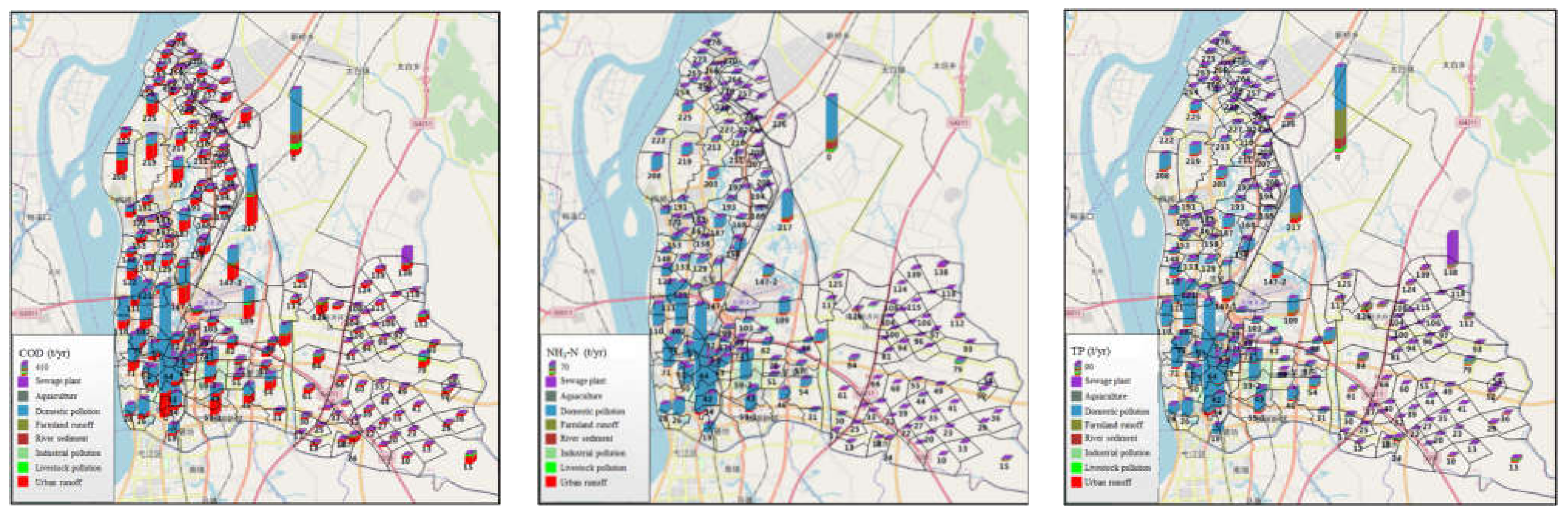
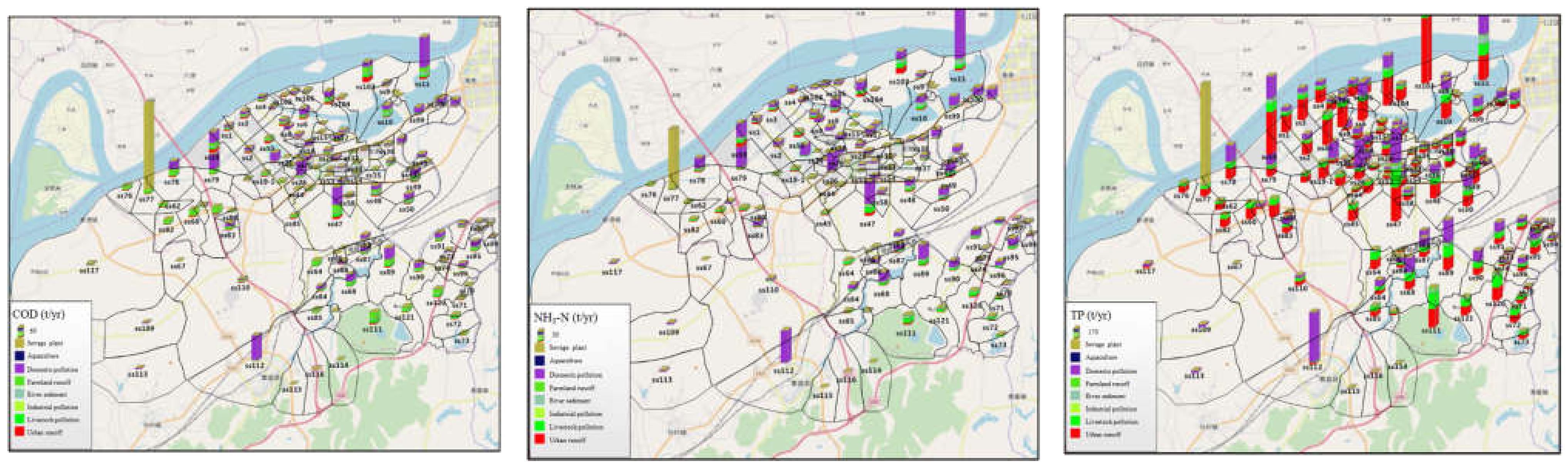
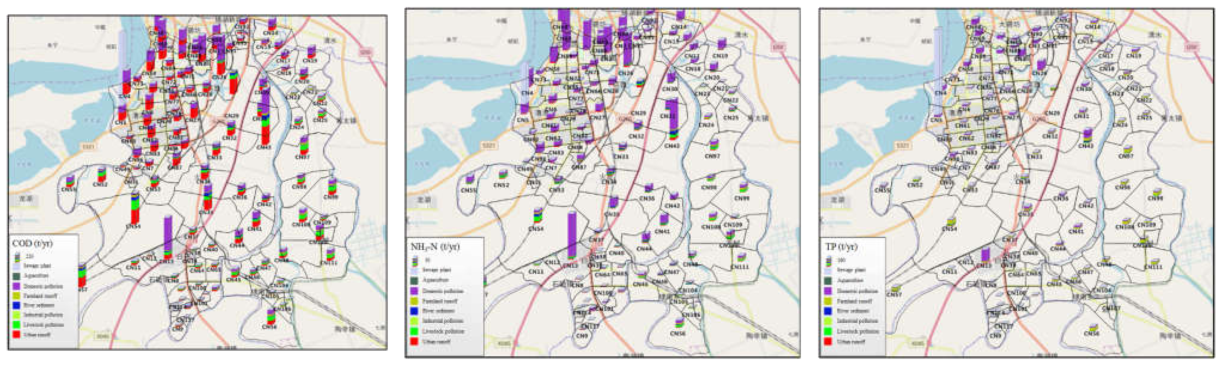
3.2.2. Source Distribution

By combining the model output results of the study scope, the amount of the total pollution load distribution by source and the amount of water entering the river were obtained, as shown in Figure 7 and Figure 8. In the annual pollution load, domestic pollution (40.85%–58.56%) accounted for the highest proportion, followed by urban surface runoff pollution (5.96%–25.92%) and breeding pollution (18.88%–23.01%). Among the annual pollution load into the river, domestic pollution (39.63%–58.68%) accounted for the highest proportion, followed by urban surface runoff pollution (3.50%–27.36%) and sewage treatment plant tail water (12.52%–22.35%). This meant that the domestic pollution and the urban surface runoff pollution were the main pollution sources of Wuhu City, and the control of domestic pollution direct discharge and NPS pollution is likely aneffective means to improve the water environment quality.

3.2.3. Spatial Distribution

As shown in Figure 9, a comprehensive analysis of the pollution load distribution map shows that the distribution of the different pollutants was spatially consistent. Figure 10, Figure 11 and Figure 12 show that the spatial distribution of the same pollutant was significantly different and had a close correlation with the type of land. In general, the concentration in the construction areas was higher than that in other land-use types. In addition, the concentration of pollutants in the highly urbanized Chengbei area was higher than that in the Chengnan area and the Sanshan area, as shown in Figure 9. Additionally, the spatial distribution of the pollution load into the river revealed similar characteristics, but the spatial distribution of the same pollutants varied greatly. The pollution load into the river of the Chengbei area was meaningfully higher than that of the Chengnan area and the Sanshan area. The higher pollutant production and the pollution loads into the river of the Chengbei area might be caused by the higher domestic pollution production and discharge. The spatial distribution of the pollution load indicated that the highly urbanized Chengbei area should be an important target of pollution control for Wuhu City.

4. Conclusions

COD, NH₃-N, and TP were used as examples to establish a pollution load model for the area south of the Yangtze River in Wuhu City using MIKE 11, ArcGIS, and Load Calculator software. The pollution load generation and migration in 2017 in the research area were simulated. By comparing the output results of the model, the following conclusions were obtained:

(1)

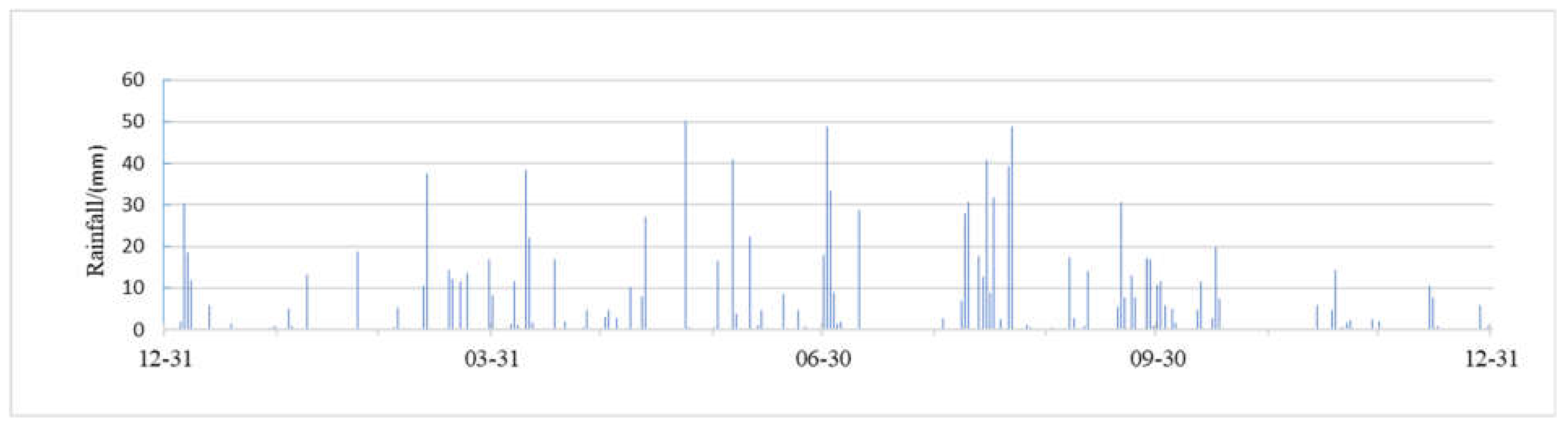
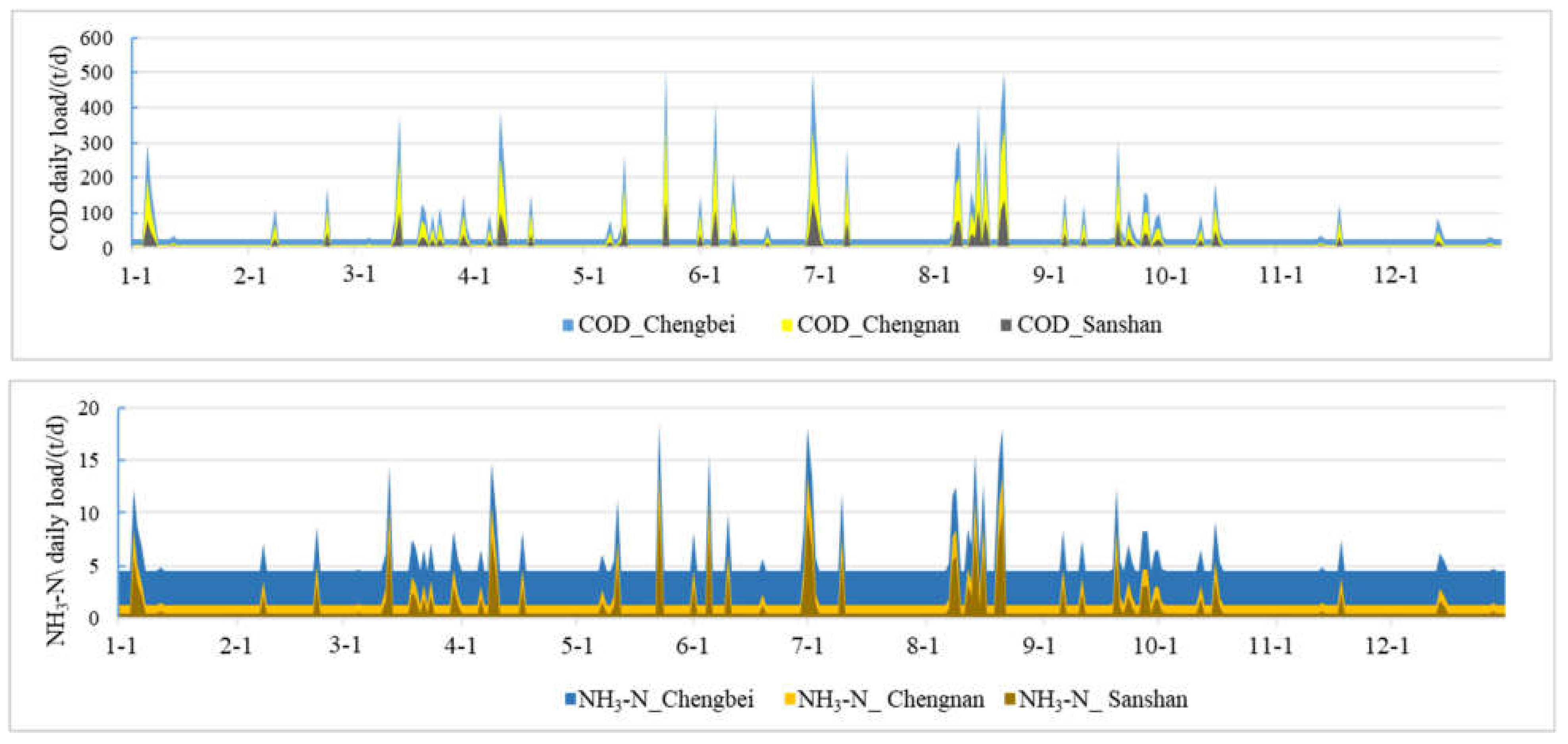
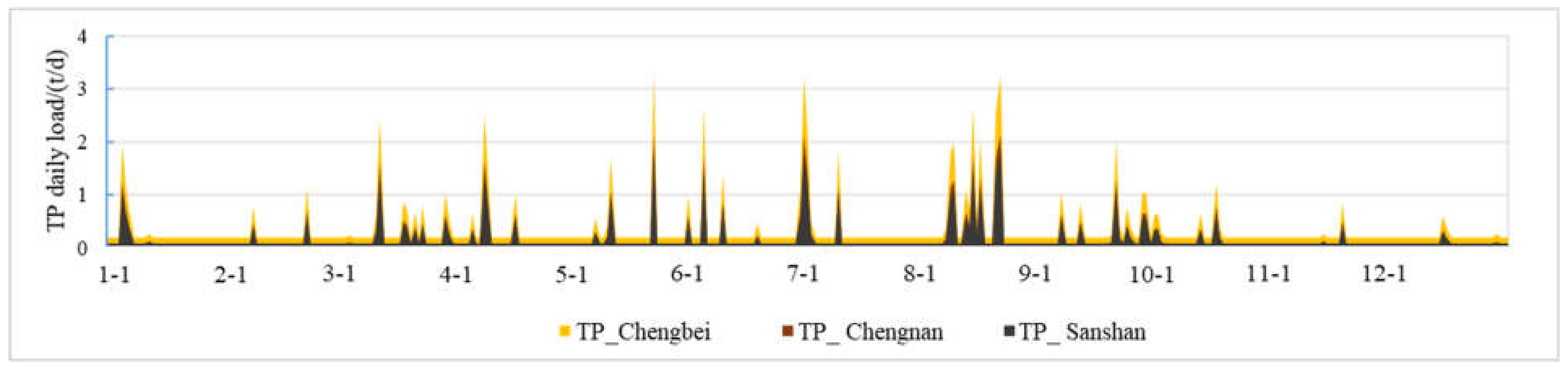
The pollutants entering the river of the study area had significant time consistency, and this was related to the rainfall events.

(2)

According to the production and migration balance system, the proportion of various pollution loads entering the river was obtained with percentages greater 25%. The proportion of COD entering the river was 32.13%. The proportion of NH3-N entering the river was 25.68%. Finally, the proportion of TP entering the river was 30.28%.

(3)

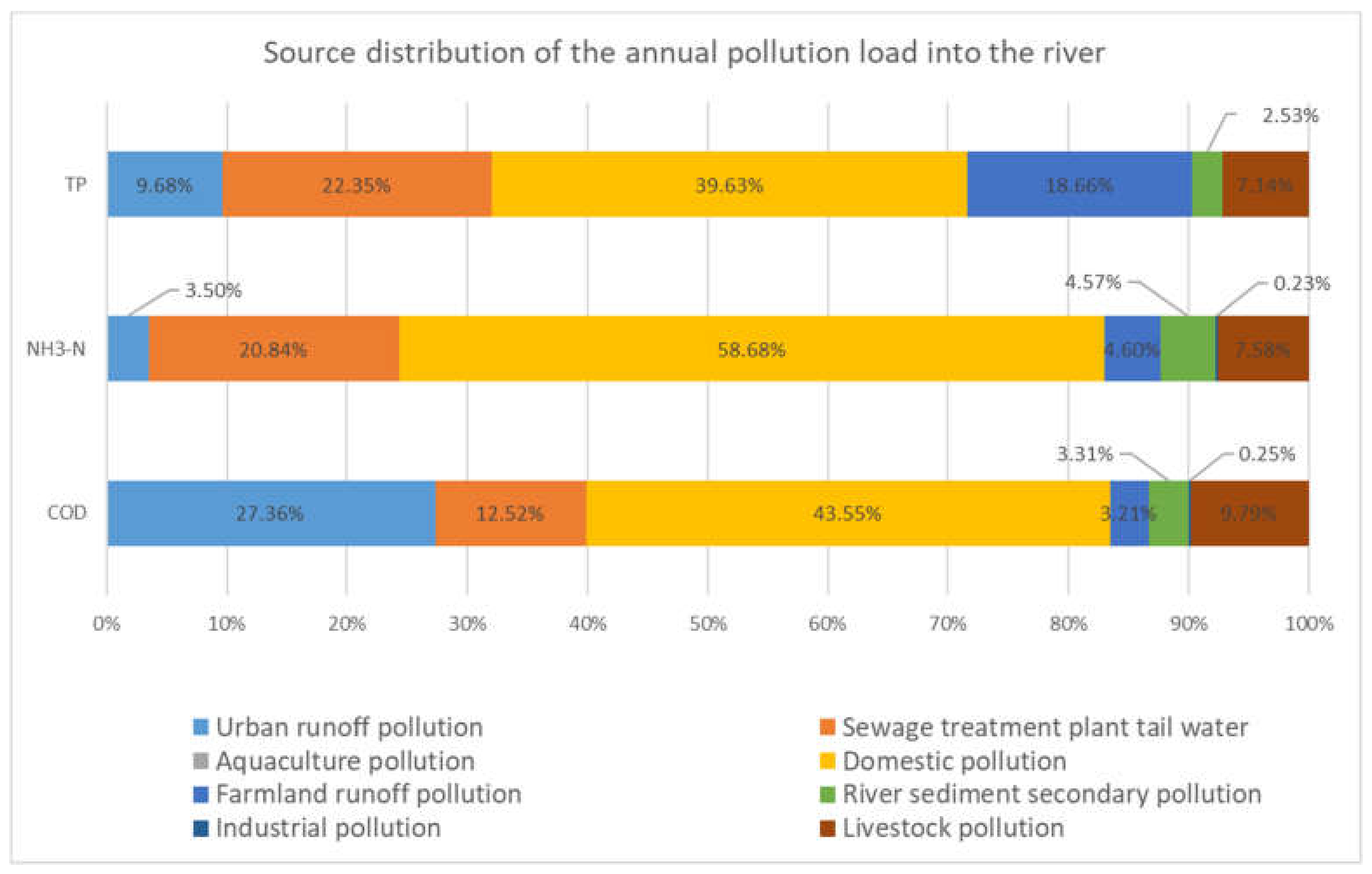
The distribution of sources revealed that the domestic pollution and urban surface runoff pollution had higher contributions to the local pollution load. It is recommended to take targeted measures against domestic pollution and urban surface runoff pollution to reduce the amount of production.

(4)

The amount of pollution load generated and the pollution load entering the river showed that the contribution from construction areas was significantly spatially higher than that of other land types. On the basis of this, it can be concluded that in order to reduce the pollution load of urban construction, planners should focus on highly urbanized areas.

(5)

The comprehensive investigation of the temporal and spatial distribution of the pollution load of Wuhu City can help guide the aquatic environmental management of Wuhu City. Meanwhile, the research methods and conclusions of this study also have reference significance for other cities along the Yangtze River and, therefore, promote the conservation of the Yangtze River and the healthy development of the Yangtze River Economic Belt.

(6)

Meanwhile, this study was conducted through the establishment of the one-dimensional river network model, and the endogenous pollution and self-purification process of the two-dimensional lake model needs further investigation.

References

1. Li, C.L.; Hu, Y.M.; Liu, M.; Tu, Y.Y.; Sun, F.Y. Urban non-point source pollution: Research progress. Chin. J. Ecol. 2013, 32, 492–500. [Google Scholar]
2. Sartor, J.; Boyd, G.; Agardy, F. Water Pollution Aspects of Street Surface Contaminants. J. Water Pollut. Control. Fed. 1974, 46, 458–467. [Google Scholar] [PubMed]
3. Collins, P.G.; Ridgway, J.W. Urban storm runoff quality in southeast Michigan. Am. Soc. Civ. Eng. 1980, 106, 153–162. [Google Scholar] [CrossRef]
4. Li, H.Z.; Zhang, M.X. A review on the calculation of non-point source pollution loads. IOP Conf. Ser. Earth Environ. Sci. 2019, 344, 012138. [Google Scholar] [CrossRef]
5. Whipple, W., Jr.; Hunter, J.V.; Yu, S.L. Effects of storm frequency on pollution from urban runoff. J. Water Pollut. Control. Fed. 1977, 49, 2243–2248. [Google Scholar]
6. Zaghloul, N.A.; Kiefa, M.A.A. Neural network solution of inverse parameters used in the sensitivity-calibration analyses of the SWMM model simulations. Adv. Eng. Softw. 2001, 32, 587–595. [Google Scholar] [CrossRef]
7. Gao, Q.X.; Li, T. Review on Nonpoint Source Runoff Quality Simulation Models in Foreign Cities. Saf. Environ. Eng. 2003, 10, 11–14. [Google Scholar]
8. Park, M.; Choi, Y.S.; Shin, H.J.; Song, I.; Yoon, C.G.; Choi, J.D.; Yu, S.J. A Comparison Study of Runoff Characteristics of Non-Point Source Pollution from Three Watersheds in South Korea. Water 2019, 11, 966. [Google Scholar] [CrossRef] [Green Version]
9. Malagó, A.; Bouraoui, F.; Pastori, M.; Gelati, E. Modelling Nitrate Reduction Strategies from Diffuse Sources in the Po River Basin. Water 2019, 11, 1030. [Google Scholar] [CrossRef] [Green Version]
10. Wang, X.Y. Non-Point Source Pollution and Its Management; China Ocean Press: Beijing, China, 2003. [Google Scholar]
11. Zhu, X.; Lu, J.X.; Bian, J.Z.; Wu, Y.F.; Han, Y.Y.; Song, J.L. Discussion on the characteristics of non-point source pollution of farmland runoff and the quantitative method of load. Environ. Sci. 1985, 5, 6–11. [Google Scholar]
12. Shi, W.G. Discussion on Long-term Pollution Load Model of Urban Rainfall Runoff. Urban Environ. Urban Ecol. 1993, 6, 6–10. [Google Scholar]
13. Chen, M.Z.; Ruan, X.H. Research on non-point source water quality model. Shanghai Environ. Sci. 1993, 12, 4. [Google Scholar]
14. Chen, X.P. CIS model and calculation of river pollution caused by urban runoff. J. Hydraul. Eng. 1993, 2, 57–63. [Google Scholar]
15. Tao, Y.; Zhao, X.L.; Li, S.W.; Xia, J.X. On-spot study of the waste load allocation in Shenzhen Bay basin based on TMDL. J. Saf. Environ. 2013, 13, 46–51. [Google Scholar]
16. Long, T.Y.; Liu, M.; Liu, J. Development and application of non-point source pollution load model of spatial and temporal distribution in Three Gorges Reservoir Region. Trans. Chin. Soc. Agric. Eng. 2016, 32, 217–223. [Google Scholar]
17. Chen, B.H.; Chang, S.X.; Lam, S.K.; Erisman, J.W.; Gu, B.J. Land use mediates riverine nitrogen export under the dominant influence of human activities. Environ. Res. Lett. 2017, 12, 094018. [Google Scholar] [CrossRef] [Green Version]
18. Jiang, N.; Chen, Z.H.; Zhao, Z.M.; Long, Y.X.; Huang, P. Study of water pollution load prediction and pollution economic loss in coastal zone based on system dynamics: A case study of Jiangmen city. Mar. Environ. Sci. 2018, 37, 720–727. [Google Scholar]
19. Zhang, Z.; Huang, P.; Chen, Z.H.; Li, J.M. Evaluation of Distribution Properties of Non-Point Source Pollution in a Subtropical Monsoon Watershed by a Hydrological Model with a Modified Runoff Module. Water 2019, 11, 993. [Google Scholar] [CrossRef] [Green Version]
20. Ren, J.S. Prediction Method of Total Pollution Load of Drinking Water Source Based on Multi-phase Remote Sensing Images. Environ. Sci. Manag. 2020, 45, 98–102. [Google Scholar]
21. Li, M.; Guo, Q. SWAT Model Simulation of Non-Point Source Pollution in the Miyun Reservoir Watershed. IOP Conf. Ser. Earth Environ. Sci. 2020, 428, 012075. [Google Scholar] [CrossRef]
22. Xie, P.; Gong, J.; Chen, C. Analysis of pollution load characteristics and control zones division of agricultural non-point sources in Beijing City. J. Environ. Eng. Technol. 2020, 10, 613–622. [Google Scholar]
23. Zhao, N.R. Discussion on Urban Surface Pollution Load Calculation and Prevention and Control Measures—Case of Kunming. Water Purif. Technol. 2021, 40, 71–75. [Google Scholar]
24. Liu, Q.M.; Zeng, J.N.; Wu, H.Y.; Rong, Q.Q.; Yue, W.C. Characteristics of runoff pollution in a highly urbanized region: A case study in the Dongguan City. E3S Web Conf. 2021, 236, 03004. [Google Scholar] [CrossRef]
25. Zong, M.; Hu, Y.m.; Liu, M.; Li, C.l.; Wang, C.; Liu, J.X. Quantifying the Contribution of Agricultural and Urban Non-Point Source Pollutant Loads in Watershed with Urban Agglomeration. Water 2021, 13, 1385. [Google Scholar] [CrossRef]
26. Wang, J. Calculation of river pollution load in plain area of middle and lower reaches of Liaohe river based on generalized model method. Water Resour. Plan. Des. 2021, 11, 56–60. [Google Scholar]
27. Polyakov, V.; Fares, A.; Kubo, D.; Jacobi, J.; Smith, C. Evaluation of a non-point source pollution model, AnnAGNPS, in a tropical watershed. Environ. Model. Softw. 2007, 22, 1617–1627. [Google Scholar] [CrossRef]
28. Chen, W.J.; He, B.; Nover, D.; Duan, W.L.; Luo, C.; Zhao, K.Y.; Chen, W. Spatiotemporal patterns and source attribution of nitrogen pollution in a typical headwater agricultural watershed in Southeastern China. Environ. Sci. Pollut. Res. 2018, 25, 2756–2773. [Google Scholar] [CrossRef] [PubMed]
29. Xu, Z.X.; Pang, J.P.; Liu, C.M. Assessment of runoff and sediment yield in the Miyun Reservoir catchment by using SWAT model. Hydrol. Processes 2009, 23, 3619–3630. [Google Scholar] [CrossRef]
30. Danish Hydraulic Institute. Manual for Load Calculator; Danish Hydraulic Institute: Copenhagen, Denmark, 2018. [Google Scholar]
31. Huang, L. Estimation Method of Water Environment Capacity and Target Reduction Amount: A Case Study of Liangtan River Basin in Chongqing. Ecol. Environ. Monit. Three Gorges 2020, 5, 65–72. [Google Scholar]
32. First National Pollution Source Census Data Compilation Committee. Handbook of Pollution Source Census Production and Emission Coefficient; China Environmental Science Press: Beijing, China, 2011. [Google Scholar]
33. Zheng, L. Study on the Characteristics of Rainfall Runoff Pollution in Zhenjiang City. Ph.D. Thesis, Jiangsu University of Science and Technology, Zhenjiang, China, 2012. [Google Scholar]
34. Chen, Y.H. Research on River Water Pollution and Restoration in a Typical Town in the River Network Area of Jiangsu Province. Ph.D. Thesis, East China University of Science and Technology, Shanghai, China, 2010. [Google Scholar]
Figure 1. Research scope of the pollution load in Wuhu City.
Water 14 00386 g001
Figure 2. Model building schematic map.
Water 14 00386 g002
Figure 3. Schematic of the pollution source generation and migration.
Water 14 00386 g003
Figure 4. Model input file.
Water 14 00386 g004
Figure 5. Distribution map of the daily rainfall in Wuhu City in 2017.
Water 14 00386 g005
Figure 6. Distribution of the daily pollution load into the river.
Water 14 00386 g006aWater 14 00386 g006b
Figure 7. Source distribution of the annual pollution load.
Water 14 00386 g007
Figure 8. Source distribution of the annual pollution load into the river.
Water 14 00386 g008
Figure 9. Distribution map of the total pollution load.
Water 14 00386 g009
Figure 10. Distribution of the pollution load into the river in the Chengbei area.
Water 14 00386 g010
Figure 11. Distribution of the pollution load into the river in the Chengnan area.
Water 14 00386 g011
Figure 12. Distribution of the pollution load into the river in the Sanshan area.
Water 14 00386 g012