Article

Application of a Developed Numerical Model for Surfactant Flushing Combined with Intermittent Air Injection at Field Scale

1
SG Institute of Environment Science & Technology, Gunsan City 54012, Korea
2
Korea Institute of Geoscience and Mineral Resources, Daejeon 34132, Korea
3
Graduate Institute of Applied Geology, National Central University, Taoyuan City 320, Taiwan
4
Department of Geology, Kyungpook National University, 80 Daehak-ro, Buk-gu, Daegu 41566, Korea
*
Author to whom correspondence should be addressed.
Water 2022, 14(3), 316; https://doi.org/10.3390/w14030316
Submission received: 20 December 2021 / Revised: 17 January 2022 / Accepted: 19 January 2022 / Published: 21 January 2022
(This article belongs to the Special Issue Remediation of NAPL-Contaminated Groundwater Aquifers)

Abstract

:
Surfactant flushing with intermittent air injection, referred to as enhanced flushing, has been proposed at a site in Korea contaminated by military activity to overcome the difficulty of treatment caused by a layered geological structure. In this study, we developed a simple numerical model for exploring the effects of various physical and chemical processes associated with enhanced flushing on pollutant removal efficiency and applied it in a field-scale test. This simple numerical model considers only enhanced hydraulic conductivity rather than all of the interacting parameters associated with the complex chemical and physical processes related to air and surfactant behavior during enhanced flushing treatment. In the numerical experiment, the removal efficiency of residual non-aqueous phase liquid (NAPL) was approximately 12% greater with enhanced, rather than conventional, flushing because the hydraulic conductivity of the low-permeability layer was enhanced 5-fold, thus accelerating surfactant transport in the low-permeability layer and facilitating enhanced dissolution of residual NAPL. To test whether the enhanced flushing method is superior to conventional flushing, as observed in the field-scale test, successive soil flushing operations were simulated using the newly developed model, and the results were compared to field data. Overall, the simulation results aligned well with the field data.

1. Introduction

The duration and cost of in situ treatment in an unconfined aquifer increases with increasing heterogeneity of the soil, and such treatment has limited applicability in layered subsurface structure. Additionally, it is regarded as a difficult situation for non-aqueous phase liquid (NAPL) remediation when solutes are released from the low-permeability zone due to back diffusion after primary sources are removed.
Because of the inefficiency of the conventional pumps and treatment technologies used to remediate aquifers, including the low permeability mentioned above, which are contaminated with non-aqueous phase liquid, considerable effort has been expended to develop alternative remediation technologies, such as surfactant-enhanced aquifer remediation. Shen et al. [1] measured the relative permeability of sandstone and showed that the reduction in interfacial tension associated with the addition of a surfactant caused the relative permeability of both the aqueous and oil phases to increase in a water–oil system. Moreover, Torabzadeh and Handy [2] showed experimentally that, at a certain temperature, the relative permeability of both the oil and water phases increases with decreasing interfacial tension at a given water saturation in a water–oil system. In addition to relative permeability, interfacial tension changes induced by the addition of surfactant affect the capillary pressure-saturation relationship in unsaturated flow. Desai et al. [3] evaluated the influence of surfactant on the capillary pressure-saturation relationship and reported that lower surface tension enhanced drainage from unsaturated soil.
Surface tension reduction has been exploited to allow air sparing to be used as a subsurface remediation technique, referred to as the “surfactant-enhanced air sparging” method [4,5,6]. As the surface tension reduction induced by the addition of surfactant decreased the water-holding capacity of sand, the ability of air to displace groundwater could be enhanced, thereby increasing the area of air sparging compared to that without surfactant and increasing the contact between air and NAPL. Furthermore, the flow of gas and surfactant solution through porous media results in foam generation in situ, which leads to increased viscosity and has the tendency to preferentially block channels and high-permeability regions in porous media, thus diverting gas to lower-permeability regions [7,8,9].
A few studies have used numerical modeling to investigate the mechanism of enhanced remediation associated with various physical and chemical processes involved in surfactant flushing combined with air injection [10,11]. Similarly, with the aim of enhancing oil recovery, numerical simulations have been conducted to investigate the effectiveness of SAG injection for increasing displacement efficiency; these studies have considered surfactant foam transport in terms of the gas mobility reduction and relative permeability changes associated with a reduction of interfacial tension [12,13,14,15,16,17,18,19]. However, most of these works considered only some, and not all, of the processes that improve remediation when surfactant flushing is combined with air injection. For example, Lee et al. [10] simulated foam flow process using method of characteristics (MOC)-based three-phase fractional flow theory (water, NAPL, foam), in which gas mobility reduction factor was calculated. However, they did not consider surfactant transport and interphase mass transfer of residual NAPL into the aqueous phase, such as dissolution, and they only considered a one-dimensional problem. However, Lee and Kam [11] performed MOC-based modelling and simulation of foam-enhanced oil recovery processes (EOR) in a multi-layered system. Lee and Kam [11] considered the surfactant transport advection effect but not the dispersion process. Zoeir et al. [14] simulated the foam EOR process using commercial software such as CMG STARS. The CMG STARS explicitly solves three-phase saturation equations and phase-pressure equations to account for capillary, viscous and gravitational forces affecting multiphase flow. However, in their study, surfactant transport was not explicitly considered even in homogenous porous media. Majidaie et al. [13] conducted numerical simulation using CMG STARS to investigate the potential of chemically enhanced water alternating gas injection as a new, enhanced oil-recovery method. They used alkaline, surfactant and polymer additives as a chemical slug, which is injected during the water alternating gas process to reduce the interfacial tension and simultaneously improve the mobility ratio. Additionally, due to immiscible carbon dioxide dissolution, oil viscosity reduction was simulated. However, Majidale et al. [13] did not explicitly consider surfactant transport. Hosseini-Nasab et al. [12] applied a local equilibrium with an implicit texture foam model for numerical modelling of foam flow in the sandstone rock in the presence of oleic phase. This model assumes that a local steady state of foam dynamics is reached instantaneously wherever gas and surfactant coexist in porous media. Additionally, this model calculated reduction of gas mobility due to the presence of a foaming agent and gas-relative permeability reduction, but surfactant concentration was assumed to be constant across simulation domain. In other words, surfactant transport was not considered. Commonly, all of above works simulated foam transport, interfacial tension reduction, relative permeability change, gas-phase mobility reduction, and viscosity change in their works, but did not explicitly simulate surfactant transport, or interphase mass transfer of residual NAPL phase to the aqueous phase, such as surfactant enhanced dissolution.
Although a comprehensive and sophisticated model considering all relevant processes, including foam transport, interfacial tension reduction, relative permeability change, gas-phase mobility reduction, viscosity change, surfactant-enhanced mass transfer, dissolved NAPL transport, and the capillary effect, is desirable, this would require numerous physical parameters that are not easily determined for field applications, making numerical simulations impractical to perform.
In the present study, we developed a numerical model and used it to investigate the effects of various physical and chemical processes associated with surfactant flushing and air injection on removal efficiency in a field-scale test. Here, to improve the practical application of numerical modeling, foam flooding and the increased aqueous phase relative permeability due to interfacial tension were not explicitly modeled but instead considered in the context of the increased hydraulic conductivity, which was determined simply through an aquifer test performed at the field site during the process of surfactant flushing combined with air injection. Meanwhile, the aqueous contaminant concentration and degree of contaminant removal from contaminant sites were simulated over time.
The objectives of this study were to: (1) develop a numerical model for simulating enhanced flushing to overcome difficult-to-treat contamination caused by a layered subsurface structure, (2) comparatively evaluate the results of field-scale tests and predictive models to clarify the characteristics of the remediation method, and (3) compare the results of the conventional and enhanced flushing methods to establish the superiority of the enhanced flushing method over the conventional flushing method.

2. Development of Numerical Simulation Model

The developed model uses a fractional flow-based approach to simulate two-phase flows, such as water and NAPL [20,21,22]. In order to obtain distributions of total pressure and water saturation in the fractional flow-based approach, the partial differential equation for total pressure is solved using the finite element method, and the partial differential equation for water saturation is solved using the finite element method (FEM) or Lagrangian–Eulerian method (LE). Subsequently, to account for surfactant-enhanced solubilization and surfactant solution transport, multispecies transport of dissolved NAPL and surfactant are simulated simultaneously using multispecies transport equations based on the finite element method or Lagrangian–Eulerian method. Details of mathematical descriptions for LE and of numerical formations of water-NAPL phase flow and multispecies transport are described in Supplementary Materials.

2.1. Equation Governing Multiphase Flow

The multiphase system in a porous medium is assumed to be composed of two phases: water and NAPL. For simplicity, we consider only incompressible fluids. The equations describing the flow of two fluid phases in a porous medium are based on conservation of mass [20,21,22,23]:
ϕ ρ i S i t + · ρ i V i = Q i + j E i j ,     i = 1 , 2       in   Ω
V i = k r i k μ i p i + ρ i g z ,       i = 1 , 2
where ρ i is the density of phase i [M L−3] (with the subscript i indicating the phase (1 for water and 2 for NAPL)), ϕ is the effective porosity of the porous medium [L3 L−3], S i is the saturation of phase i [L3 L−3], t is time [T], Q i is the source and sink term for phase i [M L−3 T−1], E i j is the rate of mass exchange from phase j to phase i [M L−3 T−1], V i is the Darcy velocity of phase i [L T−1], k r i is the relative permeability of phase i [dimensionless], k is the intrinsic permeability tensor [L2], μ i is the dynamic viscosity of phase i [M L−1 T−1], p i is the pressure of phase i [M L−1 T−2], g is the gravitational constant [L T−2], z is elevation [L] and Ω is an interested bounded area. Relative permeability relationships corresponding to the van Genuchten model are expressed as:
k r 1 = S ¯ 1 1 / 2 1 1 S ¯ 1 1 / m m 2
k r 2 = S ¯ 2 1 / 2 1 S ¯ 1 1 / m m 1 S ¯ 1 + S ¯ 2 1 / m m 2
where m is the curve shape parameter. The capillary-pressure–saturation relationship in the water-NAPL phase system follows the model of Parker et al. [24], as follows:
S 1 ¯ = 1 + α 21 h 21 n m ,       if   h 21 > 0
S 1 ¯ = 1 ,       if   h 21 0
where n [dimensionless] and α 21 [L−1] are the van Genuchten parameters and h 21 = h 2 h 1 is the NAPL-water capillary head [L], h 1 is the pressure head of water phase [L] and h 2 is the pressure head of NAPL phase [L]. S 1 ¯ and S 2 ¯ are water and NAPL saturations, respectively, and are defined as follows:
S 1 ¯ = S 1 S 1 r 1 S 1 r ,       S ¯ 2 = S 2 S 2 r 1 S 2 r
where S 1 r is the irreducible saturation of the water phase [dimensionless] and S 2 r is the residual NAPL saturation [dimensionless]. The total velocity, V t [L T−1], given by the sum of the velocities of the two phases, is defined as follows:
V t = V 1 + V 2
Using Equations (2) and (8), it can be rewritten as:
V t = i = 1 2 k r i k μ i p i + ρ i g z
Based on Equation (9), we can define the total mobility, κ [L3 T M−1]; fractional mobility for phase i , κ i ; and mobility-weighted average fluid density [dimensionless], ρ ¯ [M L−3] as follows:
κ = i = 1 2 k r i k μ i
κ i = k r i μ i j = 1 2 k r j μ j ,     i = 1 , 2
ρ ¯ = κ 1 ρ 1 + κ 2 ρ 2
Substituting Equations (10)–(12) into Equation (9) results in:
V t = κ 1 2 p 1 + p 2 + κ 1 κ 2 2 p 1 p 2 κ ρ ¯ g z
where κ 1 + κ 2 = 1 . If we define the total pressure, P t [M L−1 T−2], of an imaginary variable as follows:
P t = p 1 + p 2 2 + 1 2 0 p 1 p 2 κ 1 κ 2 d η
Equation (13) becomes:
V t = κ · P t + ρ ¯ g z
The total pressure in the water and NAPL two-phase system is calculated as follows [20,21,22]:
· κ · P t + ρ ¯ g z = Q 1 ρ 1 + Q 2 ρ 2 + E n w ρ 1 E n w ρ 2   in   Ω
where E n w is the mass exchange from the NAPL to the water phase [M L−3 T−1]. Initial and boundary conditions of total pressure equation can be transformed according to numerical schemes provided by Suk and Yeh [21]. In Equation (16), the total mobility, κ [L3 T M−1], is an independent parameter of the total pressure, P t [M L−1 T−2], and the equation is linear. The velocities of the water and NAPL phases determined using Equation (13) are as follows:
V 1 = κ 1 V t κ 1 κ κ 2 P c 12 κ 1 κ ρ 1 ρ ¯ g z
V 2 = κ 2 V t κ 2 κ κ 1 P c 21 κ 2 κ ρ 2 ρ ¯ g z
where P c 12 P c 21 [M L−1 T−2] is the capillary pressure of water (NAPL) and NAPL (water). Assuming incompressible flow and continuity of the total flux, Equation (17) can be substituted into the water-phase mass conservation Equation (1), resulting in the following water saturation equation:
ϕ S 1 t + V t · d κ 1 d S 1 S 1 = · κ 1 κ κ 2 P c 12 S 1 · S 1 κ 1 · V t + · κ 1 κ · ρ 1 ρ ¯ g z + Q 1 ρ 1 + E n w ρ 1
Initial and boundary conditions of water saturation equation can be obtained according to numerical schemes provided by Suk and Yeh [21]. In the fractional flow formulation, water saturation Equation (19) has the properties of transport equation with mixed parabolic and hyperbolic properties of the partial differential equation. Even though the water saturation equation can be solved using the standard FEM, problems such as spurious oscillation, numerical dispersion, grid orientation, phase error, peak clipping and valley elevating might be encountered. To avoid the numerical problems, a LE approach can be additionally used in this study. Details of LE approach for water saturation equation are described in Supplementary Materials.

2.2. Transport Equations for Dissolved NAPL Species and Surfactant

The transport behavior of a dissolved contaminant can be described based on adsorption and surfactant-enhanced dissolution from the NAPL to aqueous phase by considering linear adsorption and mass conservation equation of a dissolved contaminant, as follows:
θ 1 + ρ b K d , o C o t + V 1 · C o · θ 1 D · C o + Q 1 ρ 1 C o = E n w
where C o is the concentration of the dissolved contaminant [M L−3], ρ b is the bulk density [M L−3], θ 1 is the water content [L3 L−3], K d , o is the distribution coefficient between adsorbed and aqueous NAPL species [L3 M−1], and Q 1 is the source and sink term for water [M L−3 T−1]. θ 1 D is the dispersion coefficient [L2 T−1], which is defined as follows:
θ 1 D = α T V 1 δ + α L α T V 1 V 1 V 1 + θ 1 a m τ δ
where V 1 is the magnitude of V 1 [L T−1]; δ is the Kronecker delta tensor; α L and α T are the longitudinal and transverse dispersivities [L], respectively; a m is the molecular diffusion coefficient [L2 T−1]; and τ is the tortuosity [dimensionless]. The mass exchange rate from the NAPL phase to the water phase can be determined as follows [25,26,27]:
E n w = C n w ρ n w ¯ C o
C n w = a m d p 2 S h ,   S h = β 0 R e β 1 θ 2 β 2 ,   R e = d p v 1 ρ 1 μ 1
ρ n w ¯ = ρ n , p u r e w ¯ + γ C s
where C n w is the rate coefficient, which regulates the rate at which equilibrium is reached [T−1]; a m is the molecular diffusion coefficient [L2 T−1]; d p is the mean particle diameter [L]; S h is the Sherwood number [dimensionless]; R e is the Reynolds number [dimensionless]; v 1 is the seepage velocity [L T−1]; ρ 1 is the water density [M L−3]; μ 1 is the dynamic viscosity of water [M L−1 T−1]; θ 2 is the NAPL phase volumetric content [dimensionless]; ρ n w ¯ is the equilibrium concentration of NAPL species in the water phase (solubility limit) [M L−3]; β 0 , β 1 and β 2 are dimensionless fitting parameters [dimensionless]; ρ n , p u r e w ¯ is the equilibrium concentration of NAPL species in the pure water phase [M L−3]; γ is an empirical parameter [dimensionless]; and C s is the concentration of surfactant [M L−3]. Equation (24) was formulated by Pennell et al. [28]. Equilibrium solubility is linearly related to surfactant concentration over the critical micelle concentration (CMC), as shown in Equation (24). Finally, the multiphase flow and solute transport equations can be obtained by substituting the mass exchange rate in Equation (22) into Equations (16), (19) and (20) using FEM or Equations (S18), (S21b) and (S28) using LE in Supplementary Materials.
Since the solute transport equation for the surfactant is not related to mass exchange, its governing equations can be expressed as follows:
θ 1 + ρ b K d , s C s t + V 1 · C s · θ 1 D · C s + Q 1 ρ 1 C s = 0
where C s is the surfactant concentration [M L−3], K d , s is the distribution coefficient [L3 M−1] between adsorbed and aqueous surfactant, and the solute transport equation for the surfactant using LE is illustrated in Equation (S33b) of Supplementary Materials.
The numerical procedure is presented in detail in Figure 1. First of all, the numerical simulation conducts to the total pressure P t using Equation (S36) in Supplementary Materials at step II and solves the total velocity V t using Equation (S17) at step III. Then, using the total pressure and total velocity, the water saturation S 1 is solved in Equation (S42a) for FEM or Equation (S42b) for LE at step V. Since the water saturation equation is nonlinear, the iterative process is needed to get the converged solution at step VI. After getting the converged solution of the water saturation, NAPL saturation is obtained using S 2 = 1 S 1 and water phase Darcy velocity V 1 is calculated in Equation (S19). The concentration of the dissolved contaminant C o in Equation (S27) for FEM or Equation (S28) for LE and the concentration of surfactant C s in Equation (S33a) for FEM or Equation (S33b) for LE are calculated by using Equation (S49a) for FEM or Equation (S49b) for LE, respectively, at step IX.
To validate the newly developed numerical model, dissolved NAPL transport following surfactant enhanced dissolution by surfactant flushing was used as an example. A conceptual schematic diagram of this case is shown in Figure 2, with the initial and boundary conditions indicated. The input parameters of this example were adopted from Zhong et al. [25] and are provided in Table 1. In addition, it is assumed that K d , o = K d , s = 0 , Q 1 = 0 , γ = 1 and ρ n , p u r e w ¯ = 0 .
The numerical results obtained using the developed model were compared against the analytical solution obtained by Clement [29] to verify the accuracy of the numerical solutions. As shown in Figure 3, excellent agreement was found between the numerical and analytical solutions.

3. Field-Scale Operation of Surfactant Flushing with High-Pressure Air Injection

3.1. Site Characteristics

The study site (approximately 1500 m2) was located on a military base and was contaminated with gasoline and diesel oil. The major source of petroleum contamination in the area was identified as spillage from a deteriorating oil pipeline connected to an underground storage tank. Gasoline and diesel were distributed in the subsurface at a depth of 6–9 m. The TPH concentration was analyzed using the standard method for soil in Korea. The mean TPH concentration in the area was 3010 mg/kg, which was 1.5-fold higher than the regulatory standard (i.e., 2000 mg/kg) stated in Korean soil conservation law. A hill was present in the upper part of the study site, while a sloping area and flatland were present in the lower part (Figure 4). A landfilled layer was located in the subsurface (0–6 m), and a weathered layer containing sand and completely weathered granite-based silt was present below the landfilled layer. The landfilled layer was composed of yellowish-brown sands to a depth of 6 m, and the weathered layer was composed of mixed silt and sand atop granite at depths of more than 6 m. Table 2 lists the soil characteristics of the landfilled and weathered layers in this area.

3.2. Field-Scale Remediation Operation

Recently, to resolve the problem of preferential channeling through highly permeable layers, and to remove residual oil trapped by the strong capillary forces present in highly heterogeneous layered porous media, cyclic injection of a surfactant and air has been used at a military site in Korea that was polluted with gasoline and diesel from leaking transportation pipelines. Before cyclic injection of surfactant and air, the polluted area was remediated through serial in-situ treatments, including slurping and soil flushing over a 10-month period [30]. After the long-term field operation of the serial in-situ remediation process, no free-phase NAPL was present, but residual NAPL remained.
Bio-slurping was used initially to remove about 99% of the free-phase NAPL, and in situ surfactant flushing was then conducted for 6 months to meet Korean soil conservation law. During in situ surfactant flushing, surfactant alone equivalent to 5 pore volumes was injected at a flow rate of 0.47 L/min over 3 months. However, the surfactant failed to meet Korean soil conservation law with respect to remediation because the surfactant solution could not flow through the low-permeability weathered layer sufficiently to remove residual NAPL. After the serial in-situ remediation process, the removal efficiency differed among porous layers [30]. The removal rate of total petroleum hydrocarbon (TPH) in a low-permeability weathered layer was shown to be lower than that in the high-permeability landfilled layer as the flushing solution could not move through the low-permeability weathered layer, which contained a high percentage of silt or clay; moreover, residual pollutants in the weathered layer were strongly adsorbed to the soil. Therefore, to enhance remediation in the low-permeability layer and meet the legal standard, surfactant injection combined with intermittent air injection was conducted for 12 months and was expected to increase the sweeping efficiency of the surfactant and migration ability of contaminant-laden fluids in the low-permeability weathered layer (because the surfactant foam that forms prevents preferential flow through the high-permeability layer). In addition, interfacial tension in the low-permeability layer will be reduced due to the delivery of greater amounts of surfactant into the low-permeability layer; in turn, aqueous relative permeability in the low-permeability layer will increase. For clarity, the former process (surfactant alone) is hereafter referred to as the conventional flushing method, while the latter process (surfactant with intermittent air injection) is referred to as the enhanced flushing method. The non-ionic surfactant used in this study was 0.5% Tween-80 (polyoxyethylene sorbitan monooleate). For conventional flushing, 5 pore volumes of surfactant alone were injected at a high flow rate of 0.47 L/min over 3 months. For enhanced flushing, the surfactant was injected into the aquifer at a low flow rate of 0.16 L/min, with approximately 4.4 pore volumes injected using gravity flow. Air was then injected into the low-permeability weathered layer at a high pressure of 35 psig, and at a flow rate of 350 L/min, through each air-injection well (equivalent to ~3 pore volumes). The detailed operational parameters of conventional and enhanced surfactant flushing are shown in Figure 5.
For field-scale operation, 23 surfactant solution injection wells, 8 pumping wells and 7 air-sparging wells were used, as shown in Figure 6. The radius of influence of each of the 23 surfactant wells used for soil flushing was 5.5 m, whereas the radius of influence of each of the eight pumping wells was 7.5 m. Both surfactant solution injection wells and pumping wells were installed in the subsurface (9 m depth) using 100-mm diameter PVC pipes. Screened wells were also established using pipes positioned vertically perforated at a depth of 6–9 m. Air-sparging wells were constructed from white PVC pipes, 50 mm in diameter, and these screened wells were installed to a depth of 9.0–9.5 m below the subsurface. Detailed diagrams of the surfactant-injection, pumping and air-injection wells are provided in Figure 7.

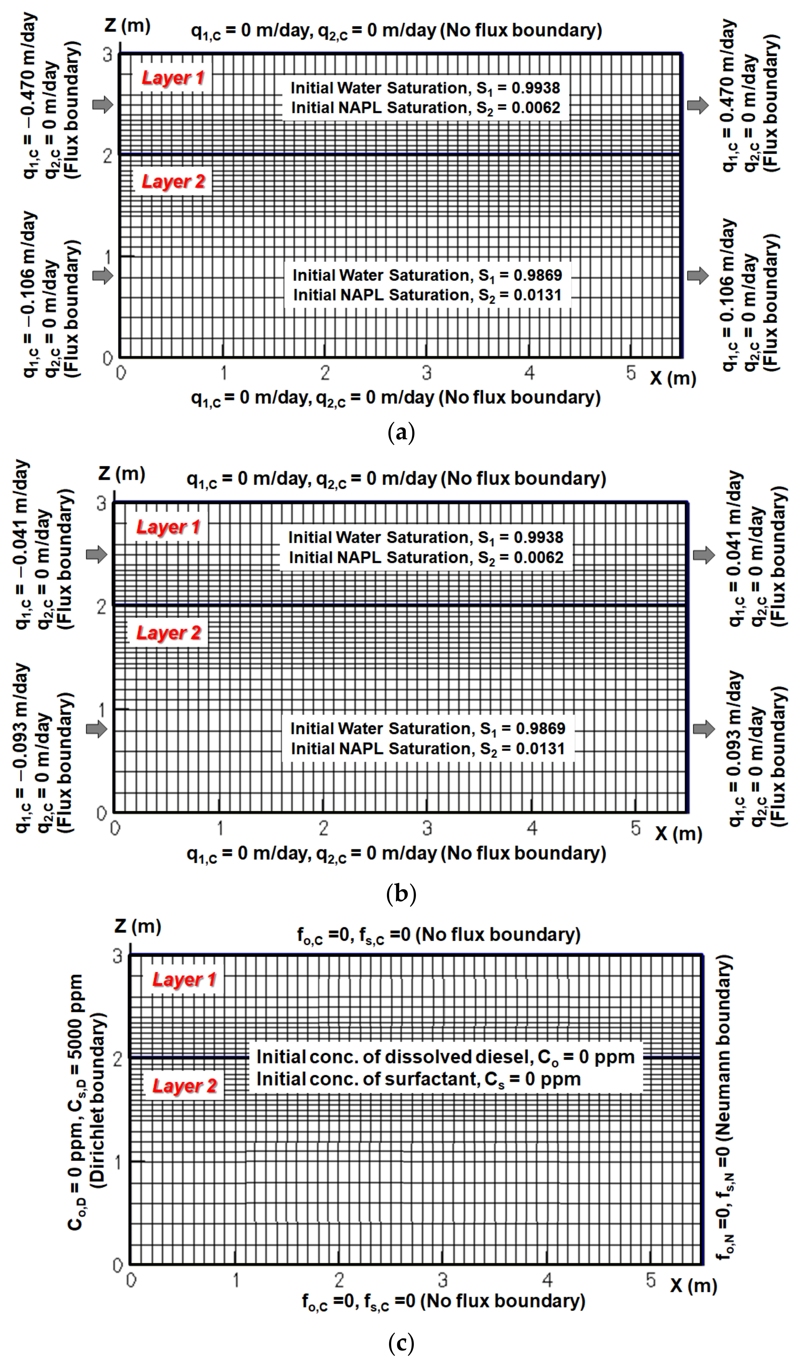
4. Numerical Experiment

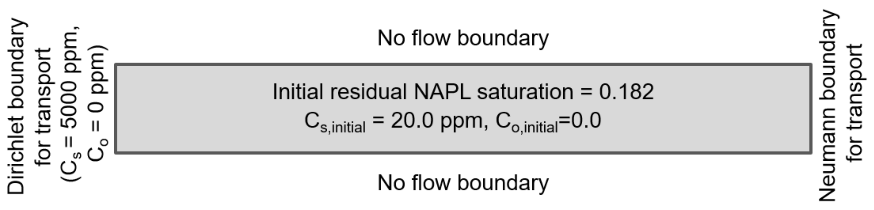
To explore the effects of high-pressure air injection during the enhanced flushing operation on remediation efficiency in the field, enhanced flushing and conventional flushing scenarios were simulated using the newly developed model to obtain concentration distributions of surfactant and dissolved NAPL over time, as well as residual NAPL saturation over time; the numerical results were compared. To reflect the aquifer and pollution distribution characteristics of the study site, the thickness of the upper layer (layer 1) was assumed to be 1 m and that of the lower layer (layer 2) to be 2 m, while the residual NAPL saturation of the upper and lower layers was set to 0.0062 and 0.0131, respectively, as shown in Figure 8. In addition, to simulate conventional and enhanced flushing under the same conditions encountered in the field, a high rate of surfactant injection (i.e., 0.47 m/day for 5 pore volumes) was assumed for an injection well at the left boundary for conventional flushing, whereas a low rate of surfactant injection (i.e., 0.16 m/day for 5 pore volumes) was assumed for an injection well at the left boundary in the enhanced flushing scenario. The input parameters associated with the aquifer properties and field characteristics of the contaminated site used for simulating the enhanced and conventional flushing scenarios are listed in Table 3. The surfactant-enhanced dissolution fitting parameters controlling non-equilibrium interphase mass transfer are provided in Table 4.
To simulate the effect of air injection during enhanced flushing on remediation efficiency, we assumed that the hydraulic conductivity of layer 2 in the enhanced flushing scenario was increased 5-fold relative to that of layer 2 in the conventional flushing scenario since delivery of surfactant into layer 2 at a lower hydraulic conductivity would be facilitated by flooding with foam formed from surfactant and air. This foam flooding would reduce interfacial tension as the surfactant in layer 2 would decrease the capillary pressure, in turn leading to increased hydraulic conductivity in layer 2 (consistent with previous research). Moreover, it has been reported that in the study area, the average hydrological conductivity was increased about 4–5-fold relative to the level prior to enhanced flushing, based on slug tests carried out in three monitoring wells after the enhanced flushing operation [31]. Further evidence of this hydraulic conductivity increase is provided by the results of a field hydraulic test, in which the zone of influence of air injection increased about 5-fold after the enhanced flushing operation [31]. Accordingly, all input parameters in Table 3 used the same values in both the conventional and enhanced flushing scenarios, except the hydraulic conductivity of layer 2.

5. Simulation Results

In this section, the NAPL saturation and the concentrations of the dissolved contaminant and surfactant are calculated. For this simulation, initial and boundary conditions for flow simulation of conventional flushing are presented in Figure 8a, for flow simulation of enhanced flushing in Figure 8b, and for solution transport of dissolved contaminant and surfactant in Figure 8c. Here, the main dominant flow of surfactant and dissolved NAPL species would be directed from the injection well to the pumping well through two horizontal layers, so the lateral migration of the chemical species for the x-z cross section was estimated to be relatively small compared to the migration along the direction aligned with the injection and pumping wells. In addition, since the purpose of this modeling was to compare the relative difference in remedial efficiency between the conventional flushing approach and the proposed improved flushing approach, we inferred that two-dimensional simulation did not cause significant errors in investigating the difference between the two flushing approaches compared to three-dimensional simulation. Accordingly, we employed two-dimensional simulation scenarios in this study without great loss of confidence.
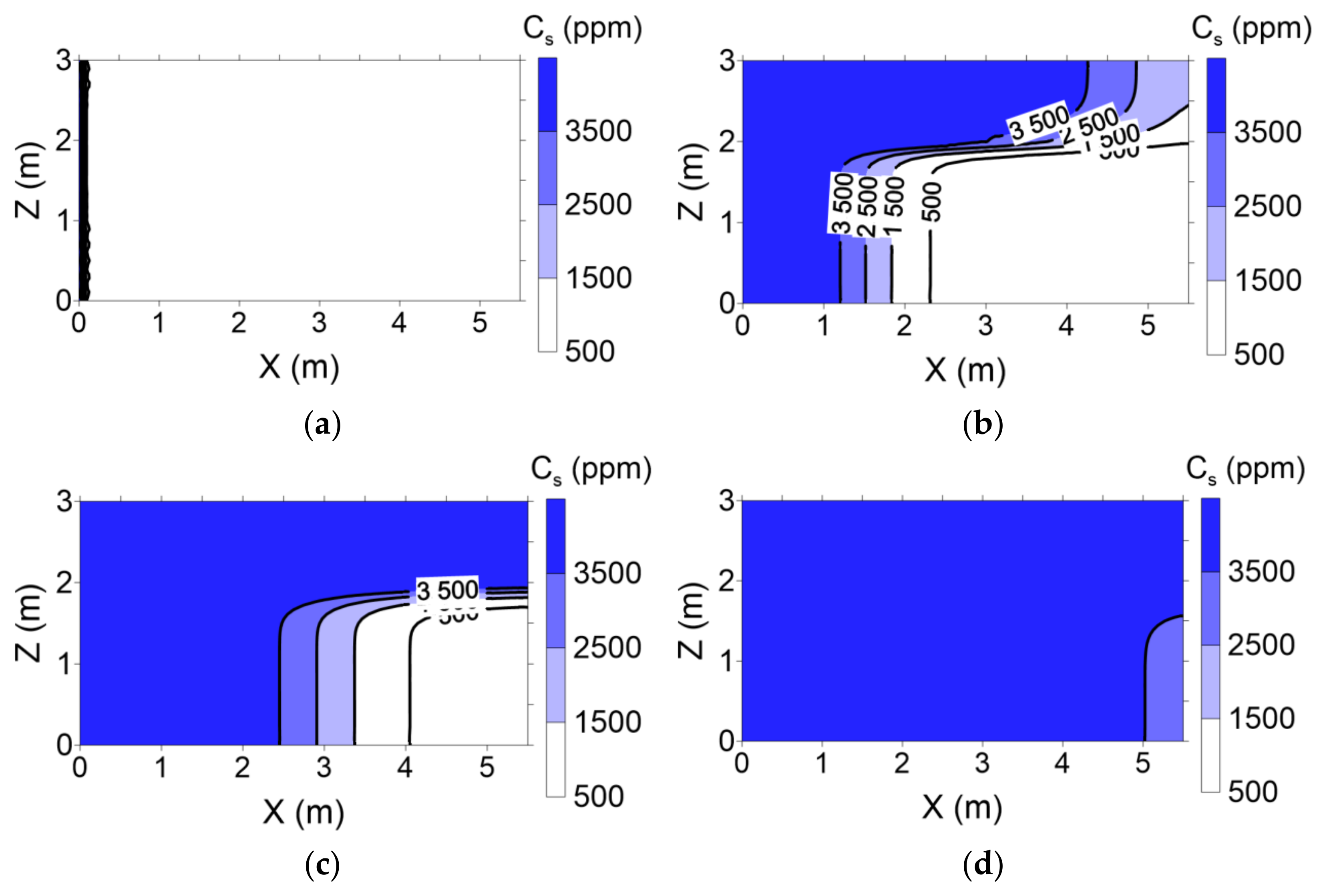
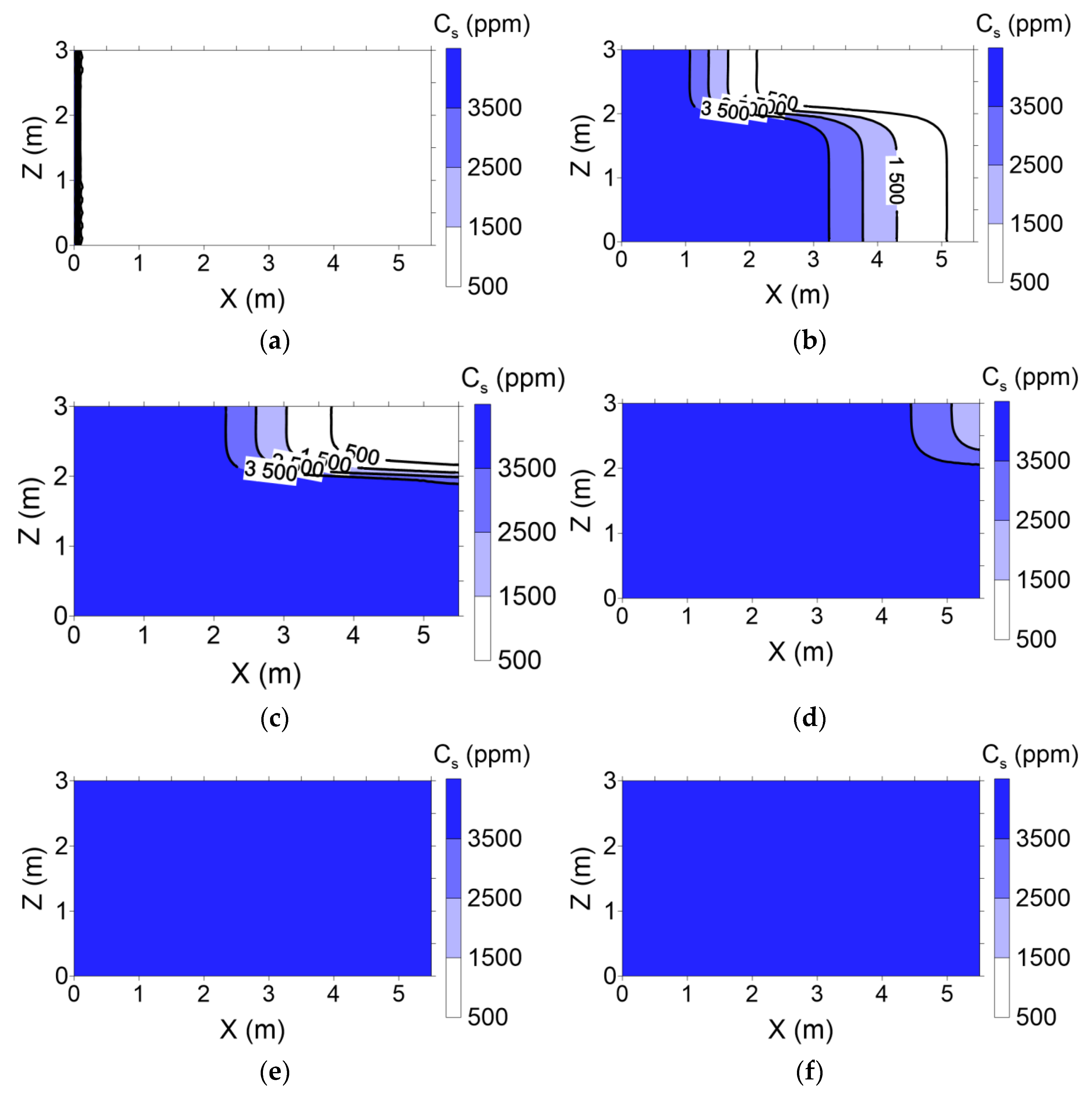
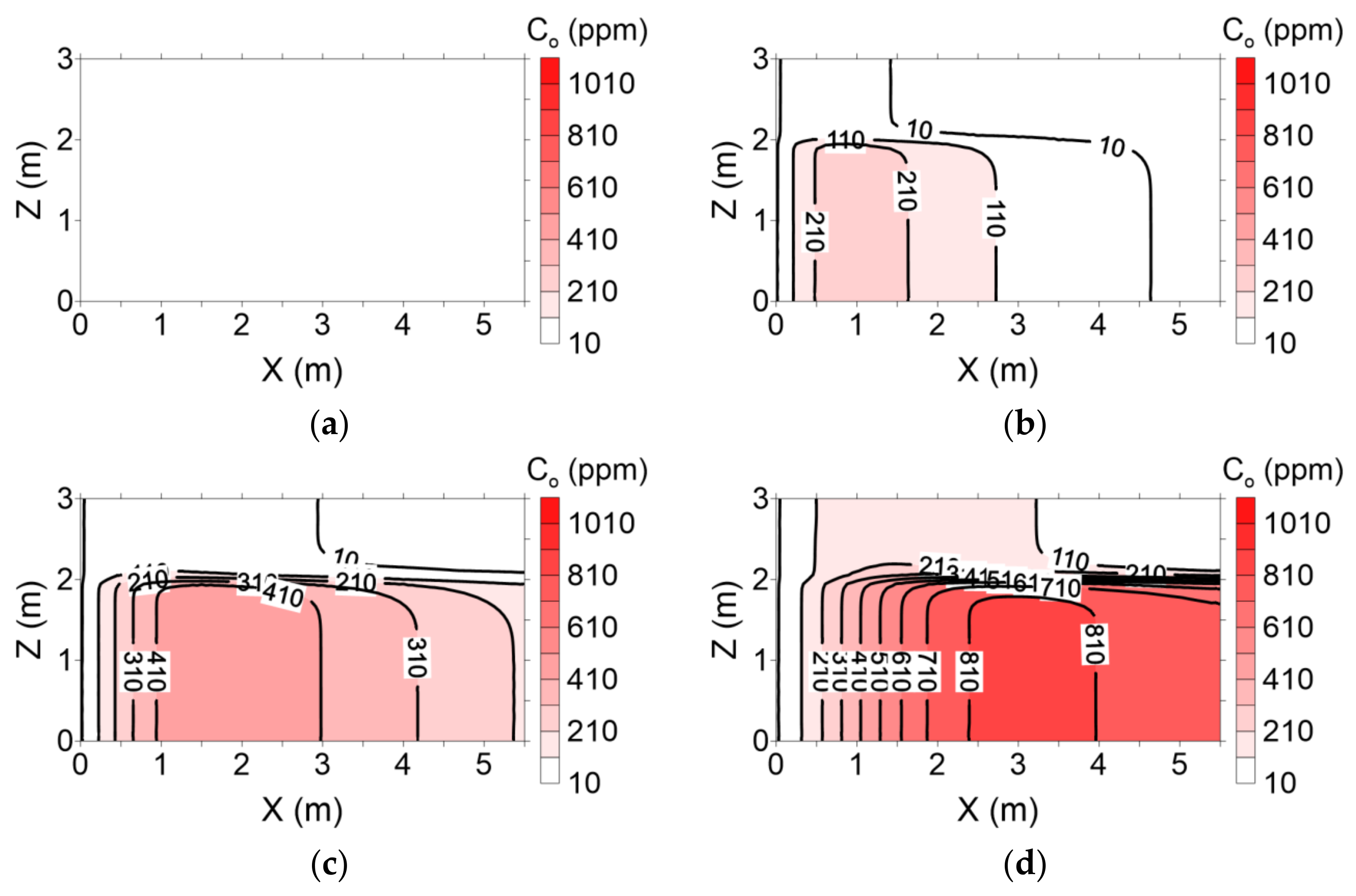
Surfactant concentration profiles with various pore volumes for conventional and enhanced flushing are shown in Figure 9 and Figure 10, respectively. In the conventional flushing scenarios, the hydraulic conductivity of layer 1 was 3-fold higher than that of layer 2 (Table 3), indicating that the surfactant injected into layer 1 moved more rapidly than that injected into layer 2. The surfactant was completely distributed through layers 1 and 2 at approximately 2 pore volumes (Figure 9). In contrast, the hydraulic conductivity of layer 1 was lower than that of layer 2 due to air injection in layer 2 in the enhanced flushing scenarios, resulting in rapid movement of the surfactant in layer 2 (Figure 10).
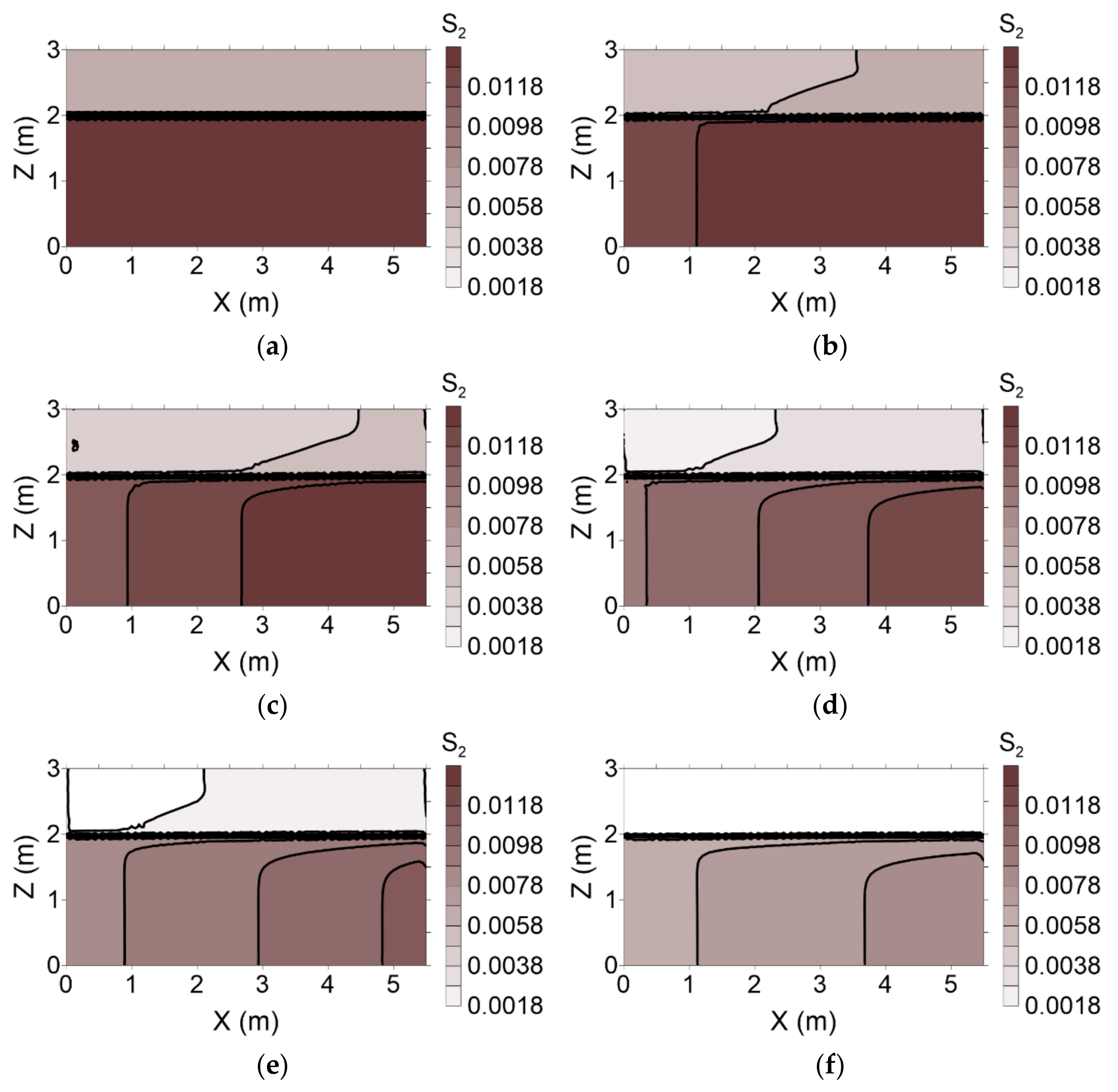
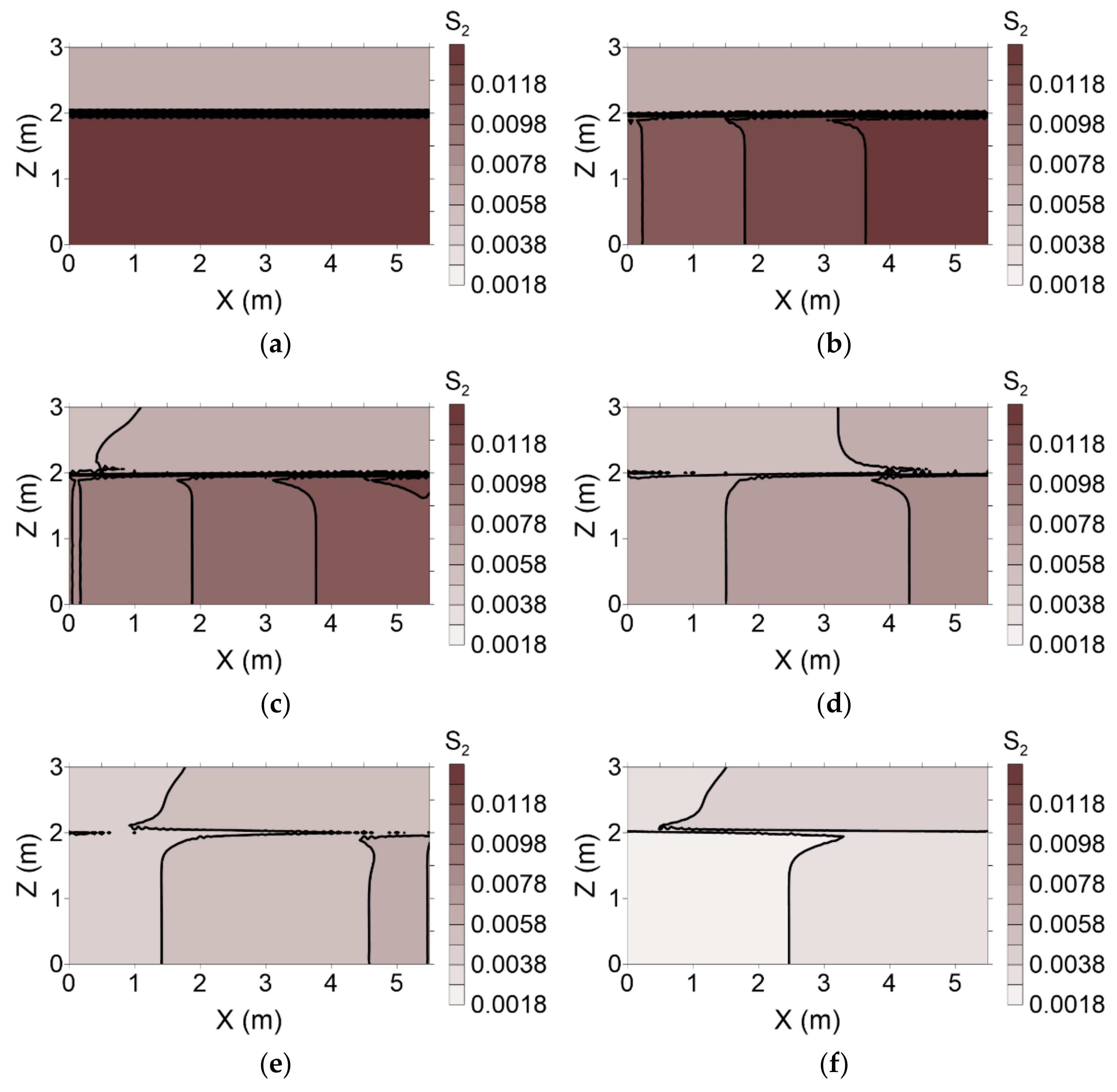
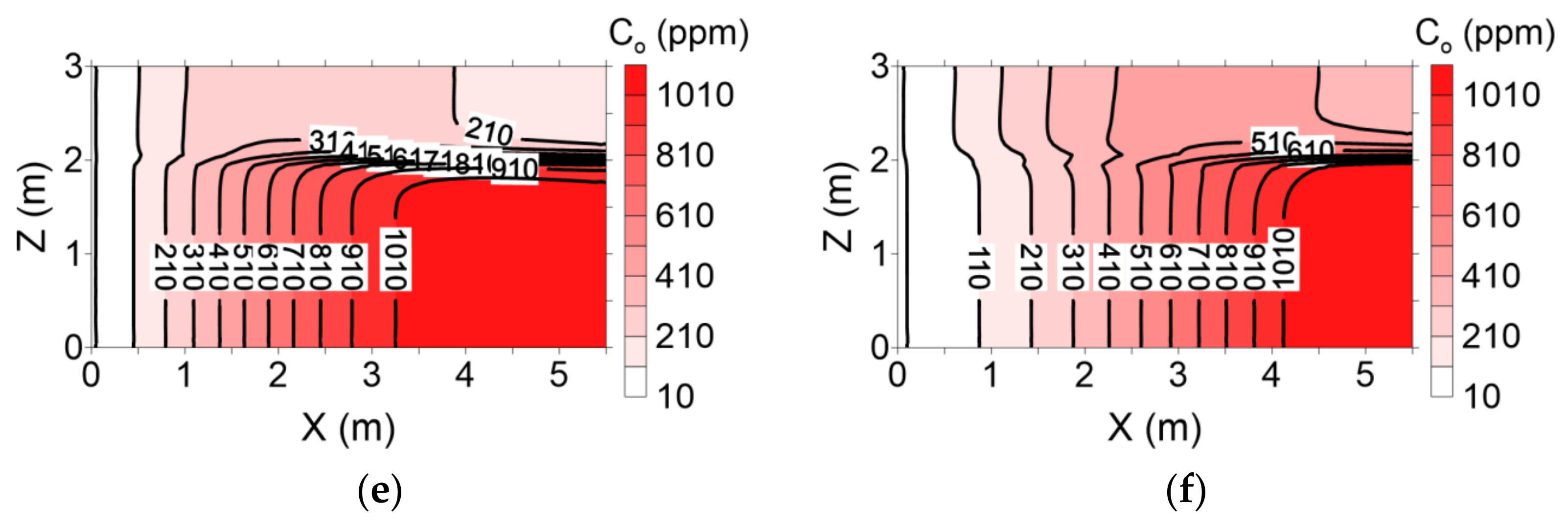
The distributions of residual NAPL saturation following surfactant injection during both flushing operations are presented in Figure 11 and Figure 12, respectively. With conventional flushing, surfactant injected into layer 1 moved more rapidly than that injected into layer 2. This result indicates that the surfactant facilitated dissolution of the residual NAPL. Therefore, residual NAPL in layer 1 was remediated more rapidly than that in layer 2 (Figure 11). However, with enhanced flushing, the residual NAPL in layer 2 was remediated more rapidly than that in layer 1 because the surfactant in layer 2 moved more rapidly than its counterpart in layer 1 (Figure 12).
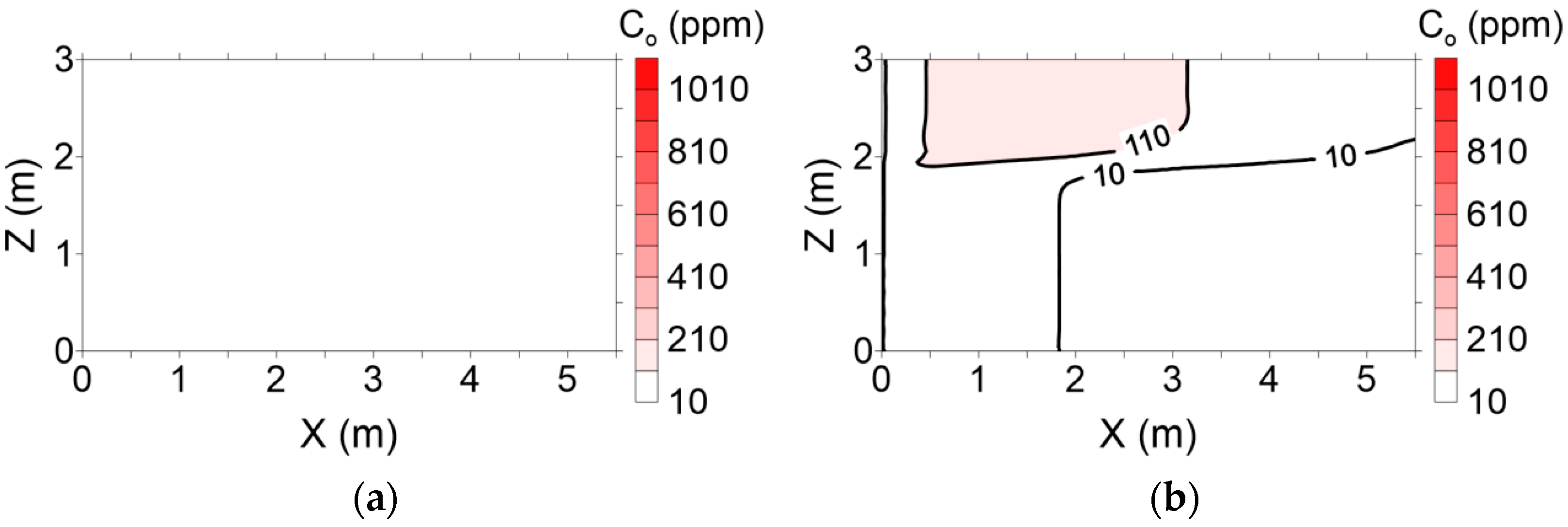
The dissolved contaminant concentrations in groundwater (i.e., the aqueous phase) following the two surfactant injection processes are shown in Figure 13 and Figure 14. A higher dissolved contaminant concentration was observed in layer 1 in conventional flushing scenario before the injection rate of three pore volumes was reached (Figure 13). Subsequently, the concentrations of dissolved contaminants increased gradually and were greater in layer 2 than in layer 1. Presumably, this difference arose because the residual NAPL in layer 1 was entirely remediated, whereas a large quantity of residual NAPL remained in layer 2 beyond 3 pore volumes (
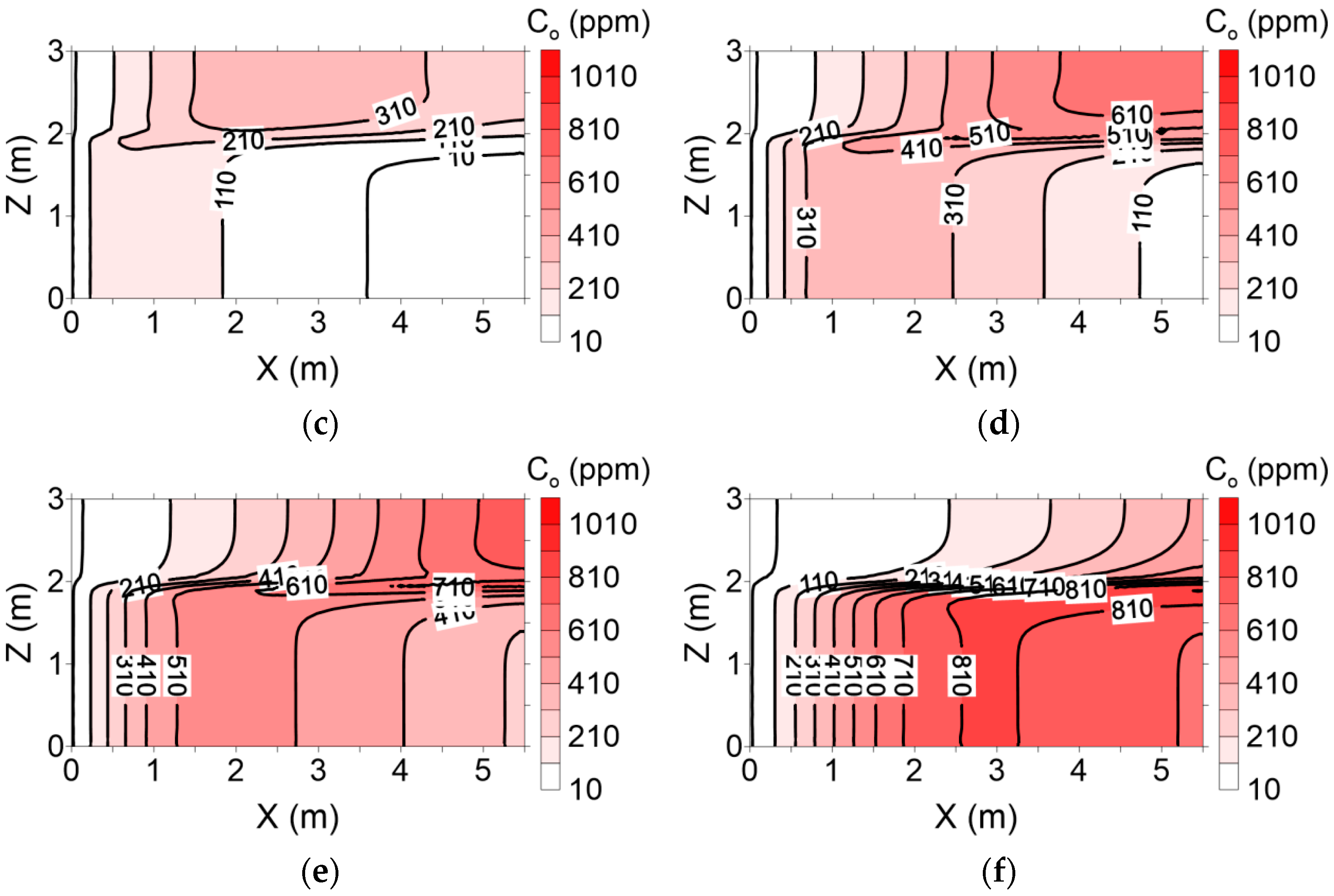
Figure 11). The dissolved contaminant concentrations of the groundwater in layers 1 and 2 were fairly high for all pore volumes tested in the enhanced flushing scenario (Figure 14). This similarity is presumably due to the presence of residual NAPL in both layers (Figure 12).
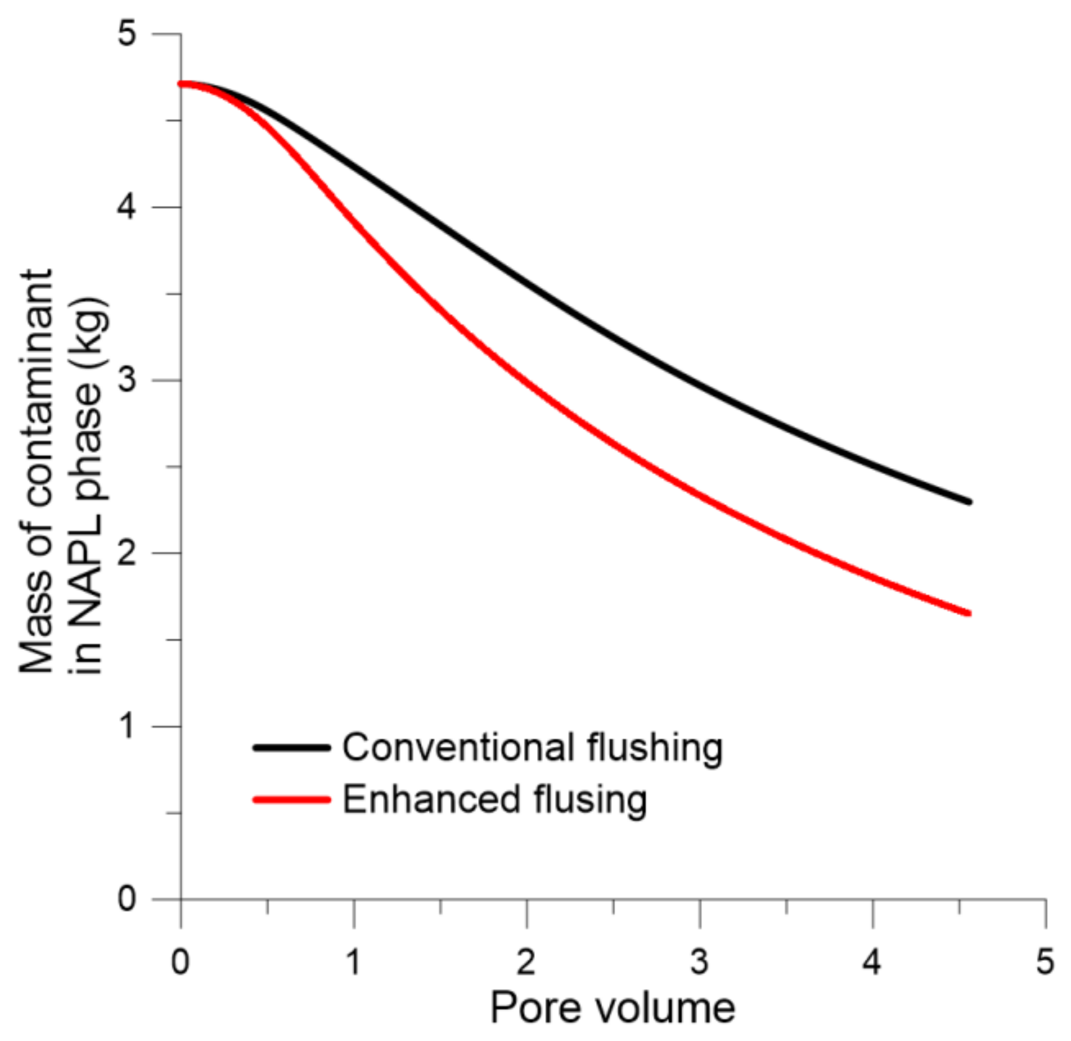
Figure 15 shows the total mass of residual NAPL in soil according to pore volume in the conventional and enhanced flushing scenarios. The removal efficiency of residual NAPL was approximately 12% greater with enhanced flushing than with conventional flushing. The difference is because the hydraulic conductivity in layer 2 with greater residual NAPL was enhanced 5-fold, as determined by field hydraulic testing. Therefore, the residual NAPL in layer 2, which had lower permeability, was remediated more efficiently.
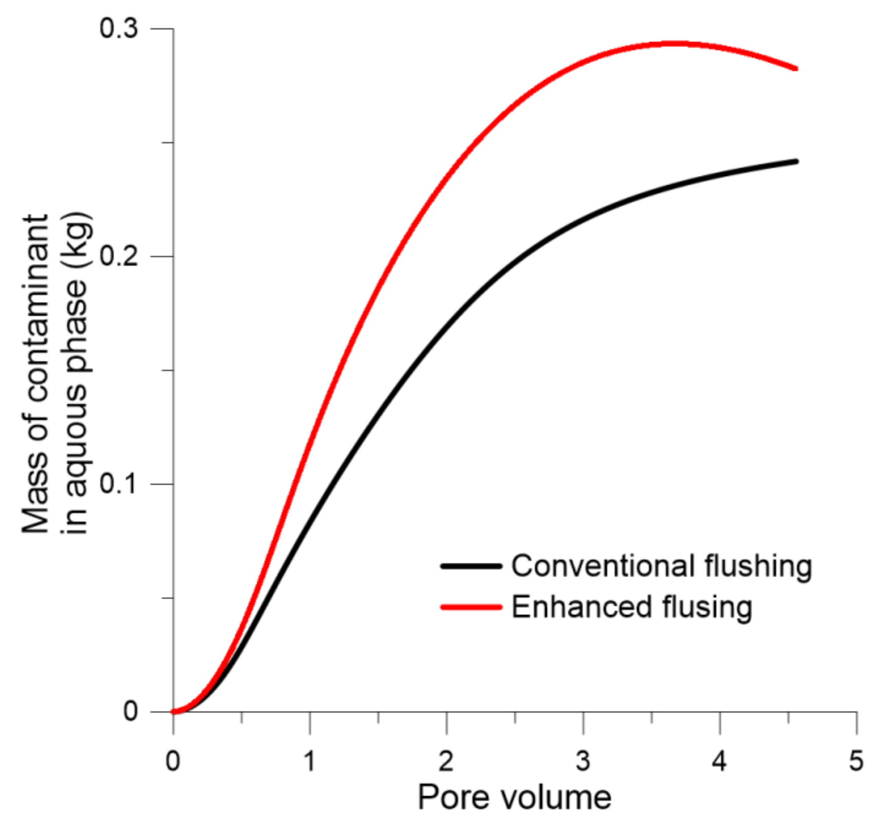
The total mass of NAPL dissolved in the aqueous phase within the pores is shown in Figure 16. In conventional flushing, the total mass of NAPL dissolved in the aqueous phase rapidly increased up to 2 pore volumes and slowly increased thereafter. As the hydraulic conductivity was higher in layer 1 than layer 2, resulting in more rapid movement of surfactant and dissolution of residual NAPL in layer 1, the level of residual NAPL in layer 1 decreased rapidly up to 2 pore volumes, as shown in Figure 11. The contaminant concentration in the aqueous phase of layer 1 increased rapidly (Figure 13). Moreover, most residual NAPL in layer 2 was removed following the nearly complete removal of residual NAPL from layer 1 at 2 pore volumes. Because the surfactant moved slowly in layer 2, the residual NAPL in layer 2 was remediated slowly; the contaminant concentration in the aqueous phase of layer 2 also increased slowly. In enhanced flushing, the total mass of NAPL in the aqueous phase decreased after reaching a maximum at 3–4 pore volumes (Figure 14). The hydraulic conductivity of layer 2, with a residual NAPL content of 68%, was enhanced 5-fold, which accelerated surfactant transport in layer 2 and facilitated the dissolution of residual NAPL in that layer through enhanced flushing. As shown in Figure 14, the contaminant concentration in the aqueous phase of layer 2 was very high at 3 pore volumes. Consequently, the total NAPL mass in the aqueous phase reached its maximum value at 3–4 pore volumes and then decreased during enhanced flushing (Figure 16).

6. Field Applications of the Enhanced Flushing and Numerical Modeling

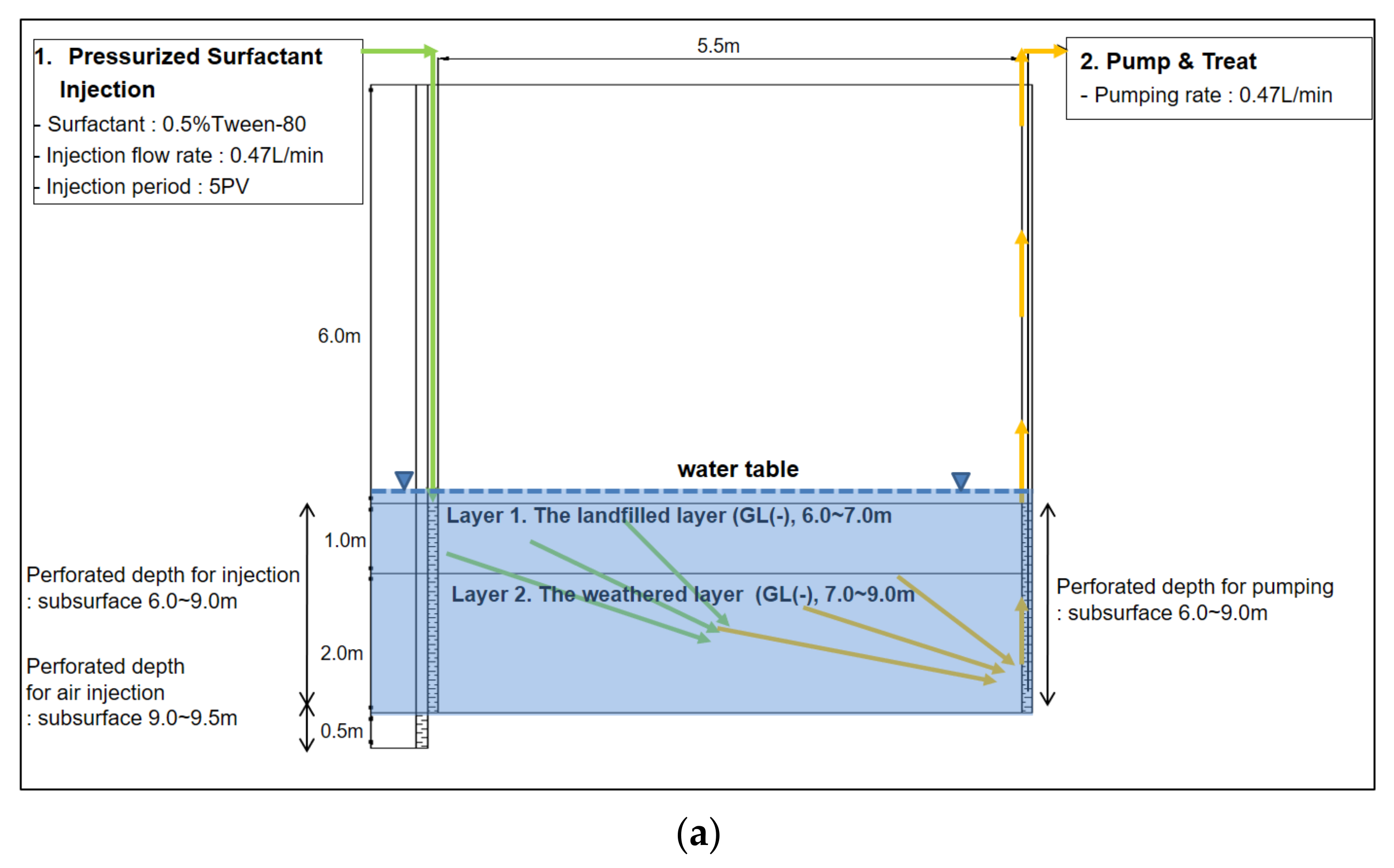
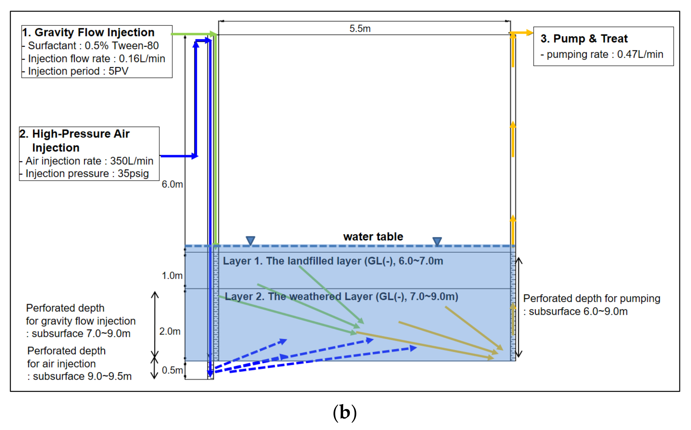
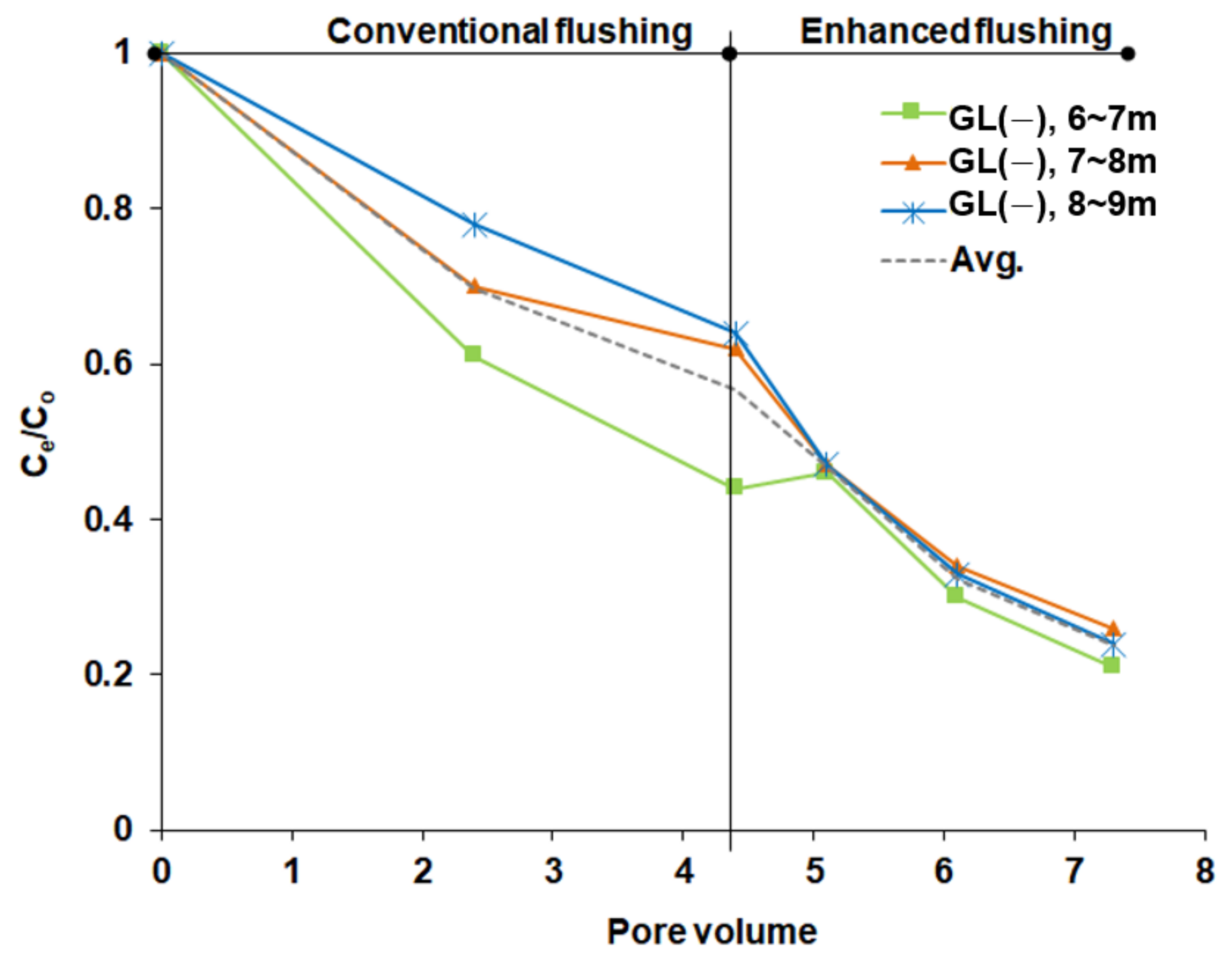
To clean up a contaminated military site in Korea to meet the Korean regulatory standard, a conventional flushing operation was performed until 4.4 pore volumes were injected at a high-flux surfactant injection rate of 0.47 L/min. Then, enhanced flushing via low-flux surfactant injection and high-pressure air injection was applied from 4.4 to 7.3 pore volumes. To compare TPH removal rates between the enhanced and conventional flushing operations at the full field scale, variations in TPH removal rates were visualized as a function of the pore volume of surfactant injected, as shown in Figure 17, when the flushing methods were applied successively. At 4.4 pore volumes, i.e., immediately after the conventional flushing operation, the TPH removal rates were 55.8%, 39.6% and 38.1% at subsurface depths of 6.0–7.0, 7.0–8.0 and 8.0–9.0 m, respectively, as shown in Figure 17. However, after 4.4 pore volumes, when enhanced flushing started, significant reductions in the TPH concentration occurred at all depths in the heterogeneous aquifer relative to conventional flushing. The TPH removal rates were 52.8%, 57.4% and 61.8% for subsurface depths of 6.0–7.0, 7.0–8.0 and 8.0–9.0 m, respectively.
In particular, a significantly enhanced removal rate was observed in layer 2 at a depth of 7–9 m, as shown in Figure 17. In conventional flushing, the lowest removal rate occurred at that depth, as surfactant solution preferentially flowed through the high-permeability layer (layer 1) rather than the low-permeability layer (layer 2).
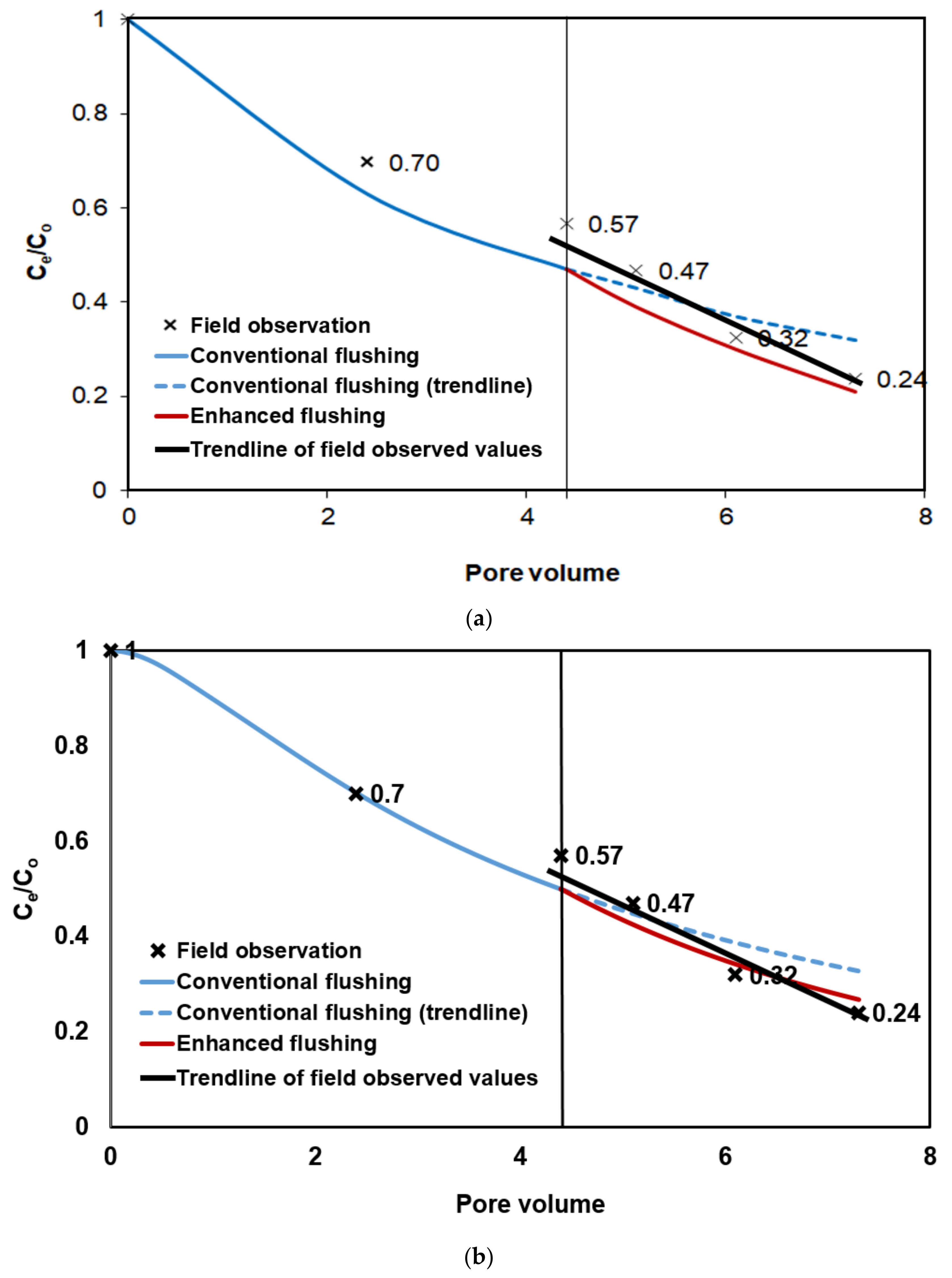
To investigate the improved removal efficiency of enhanced flushing relative to conventional flushing, we simulated successive soil flushing operations, i.e., an initial period of conventional flushing until 4.4 pore volumes followed by enhanced flushing from 4.4 to 7.3 pore volumes, and compared the simulation results against field data, as shown in Figure 18. In this simulation, the hydraulic conductivity of layer 2 during the enhanced flushing period was set to a value 5 times larger than that used with conventional flushing, to account for the interaction between air and surfactant. The effluent to initial TPH concentration ratio (Ce/Co) was determined through 7.3 pore volumes. As shown in Figure 18a, the overall simulation results showed good concordance with the field data, except at the initial time points. Initially, the simulation results showed slight underestimation compared to the field data, suggesting that the numerical simulation slightly overestimated the removal of contaminants compared to real field conditions. We had guessed that this discrepancy was produced from simply using the isotropy of hydraulic conductivity in the numerical simulation and had tried to reduce this discrepancy by considering the anisotropy. The numerical simulation was performed taking into account anisotropic cases where the vertical hydraulic conductivity of K z s in both layers is 10 times smaller than the horizontal hydraulic conductivity of K x s, respectively. However, due to top and bottom no-flux boundary conditions, we found out that there were negligible differences in vertical velocity distributions between isotropic and anisotropic cases, and in turn contaminant removal between isotropic and anisotropic cases was almost same. In addition, the top boundary condition was changed from the no-flux boundary condition to the recharge boundary condition, so that the vertical velocity distribution was changed according to the anisotropic situation. Despite the change in the top boundary conditions, the simulated contaminant removal between the isotropic and anisotropic cases in this study showed little difference. Therefore, the reason for the discrepancy between the simulation results and the observed values in this study could not be explained by the anisotropic effect alone.
Accordingly, the parameter of the mean particle size d p associated with dissolution under field conditions has been calibrated to correct a slight overestimation of numerical contaminant removal compared to actual field observations, as shown in Figure 18a. The landfill layer in this area consists of 3.6% granules, 94.1% sand and 2.3% silt/clay, while the weathering layer consists of 1.3% granules, 89.7% sand and 8.9% silt/clay (Table 2). According to Krumbein [47], granules, coarse sand and silt/clay have particle sizes of 1–5 mm, 1–2 mm and 0.002–0.1 mm, respectively. In this study, d p was calculated by multiplying each of the mean particle sizes of the soils by the percentages of each soil composition and then adding them. The d p range was estimated at 1.1–1.9 mm and 1.0–1.8 mm in landfill and weathered layers, respectively.
In order to investigate effect of the mean particle size on the dissolution, the relationship between mass exchange rate E n w and mean particle size d p can be written from Equations (22) and (23) as follows:
E n w 1 d p 2 β 1
where β 1 = 1.04 [25,27]. From Equation (26), we found out that mass exchange rate is inversely proportional to mean particle size. Therefore, in order to reduce the discrepancy between the simulated overestimated mass removal and the observed values, as shown in Figure 18a, we performed numerical calibration by gradually increasing the mean particle sizes of the landfill layer and of the weathered layer from 1.5 to 1.9 mm and from 1.4 to 1.8 mm, respectively. Finally, the numerical solutions matched best with the observations when the d p s of the landfill layer and of the weathered layer were 1.875 mm and 1.75 mm, respectively (Figure 18b). In particular, at least before 4.4 PV, the numerical solution exactly matched with the observed values. Even after 4.4 PV, the numerical simulation results of enhanced flushing were in overall good agreement with the observed values. Compared to previous smaller mean particle sizes, calibrated simulation result obtained using the larger mean particle sizes was better matched with observed values, as shown in Figure 18b. Although exact match between enhanced flushing and field observations cannot be obtained after 4.4 PV, we figured out from numerical simulation that contaminant removal rate after enhanced flushing operation was accelerated compared to conventional flushing operation before 4.4 PV, which was consistent with field observation. Therefore, in Figure 18b, slope of line in case of enhanced flushing is better matched with that of field observation trendline than slope of line in case of conventional flushing. Lastly, the small discrepancies between enhanced flushing and field observation may be still attributed to various causes such as failures to consider various wettability of geological material (contact angle), explicit surfactant foam transport, solute diffusion through immobile water films sandwiched between NAPL blobs and soil grains, and physical bypassing of mobile phases around contaminated regions.
In conclusion, the interplay between air injection and surfactant flushing during enhanced flushing gives rise to various complex chemical and physical processes that affect remediation efficiency, including surfactant foam transport, diversion of surfactant to the low-permeability layer by foam, interfacial tension reduction due to surfactant in the low-permeability layer, an increase in relative permeability, and surfactant-enhanced drainage following a reduction of capillary action and interfacial tension. To simulate all of these processes accurately, a complex, comprehensive and sophisticated numerical model would be needed, including many parameters that are not easy to measure and thus generally not suitable for field applications. However, considering only one parameter that is related to all of these processes, i.e., hydraulic conductivity, allows for the application of a simple numerical simulation to field conditions. For broader practical application of numerical modeling, further investigation of the empirical and experimental relationships of enhanced hydraulic conductivity with various processes that occur during enhanced flushing is needed.

7. Conclusions

Numerical modeling was performed using a newly developed model to predict the efficiency of contaminant removal and to elucidate the characteristics of the enhanced flushing system through comparison with other flushing methods. An enhanced flushing operation was conducted at the field scale to overcome the difficult treatment conditions associated with contamination in a heterogeneous geological setting.
To investigate the effects of high-pressure air injection during enhanced flushing on remediation efficiency in the field, enhanced and conventional flushing scenarios were simulated using the developed model to obtain concentration distributions of surfactant and dissolved NAPL over time, as well as residual NAPL saturation over time; the numerical results were compared to the field data. In the numerical experiment, the removal efficiency of residual NAPL was approximately 12% greater with enhanced flushing than with conventional flushing at 5 pore volumes because the hydraulic conductivity of layer 2, which had a residual NAPL content of 68%, was enhanced 5-fold, thus accelerating surfactant transport in layer 2 and facilitating the dissolution of residual NAPL through enhanced flushing.
At a contaminated military site in Korea, where successive soil flushing operations were performed to investigate the improved removal efficiency of enhanced flushing relative to conventional flushing, we simulated successive soil flushing operations using our newly developed model and compared the simulation results with field data. During the early stage of the conventional flushing operation, TPH removal rates at 4.4 pore volumes were 55.8%, 39.6% and 38.1% at subsurface depths of 6.0–7.0, 7.0–8.0 and 8.0–9.0 m, respectively. However, with enhanced flushing from 4.4 to 7.3 pore volumes, the TPH removal rates were 52.8%, 57.4% and 61.8% at subsurface depths of 6.0–7.0, 7.0–8.0 and 8.0–9.0 m, respectively. A significant reduction in contaminant concentration was observed regardless of depth within the heterogeneous aquifer. This enhanced removal could be simulated using the model developed in this study, as shown in Figure 18a,b. The simulations slightly overestimated contaminant removal compared to the field-scale test in Figure 18a. By performing the numerical calibration of the mean particle size and by using the larger mean particle sizes, we obtained the calibrated solutions results that accurately matched the observations in Figure 18b. This result indicated that successful simulation results can be obtained using only one parameter, i.e., enhanced hydraulic conductivity, which was identified based on the effects of various chemical and physical processes involved in the interplay between air injection and surfactant flushing, seen during enhanced flushing.
In conclusion, our field-scale test showed that low-flux injection of a surfactant, combined with high-pressure air sparging, is an effective novel method for improving the solubility and mobility of contaminants through enhancement of hydraulic conductivity. Moreover, we found that a simple numerical model considering only enhanced hydraulic conductivity rather than all of the chemical and physical processes involved in the interplay of air injection with surfactant flushing, facilitating assessment of the remediation performance of enhanced flushing technology.

Supplementary Materials

The following supporting information can be downloaded at: https://www.mdpi.com/article/10.3390/w14030316/s1. Supplementary Materials S1: Equation Governing Multiphase Flow, Supplementary Materials S2: Transport Equations for Dissolved NAPL Species and Surfactant, Supplementary Materials S3: Numerical Formulations of Water-NAPL Phase Flow and Multispecies Transport, Figure S1: Flow chart for proposed numerical method. t n + 1 and t n are new and old time levels, respectively, ∆t is time step, P t is the total pressure, S 1 and S 2 are the water phase and NAPL phase saturations, respectively, V t is the total velocity, V 1 is the Darcy velocity of water, C o and C s are the concentrations of dissolved contaminant and surfactant, respectively, V d , o and V d , s are the particle tracking velocities for dissolved contaminant and surfactant, respectively, superscripts n + 1 and n indicate the new and old time levels, respectively, superscript m is the nonlinear iteration level, and superscript * indicates the results of particle tracking.

Author Contributions

Conceptualization, H.S. and H.L.; methodology, H.S. and H.L.; software, H.S.; validation, H.S.; formal analysis, H.L. and E.P.; investigation, H.L.; writing—original draft preparation, H.S. and H.L.; writing—review and editing, H.S. and J.-S.C.; visualization, H.S. and H.L.; supervision, J.-S.C. and E.P.; funding acquisition, H.L. All authors have read and agreed to the published version of the manuscript.

Funding

The Subsurface Environment Management Project of the Korea Environmental Industry and Technology Institute (Project No.: 201800248001) and “Research on rock properties in deep environment for HLW geological disposal (GP2020-002; 21-3115)” funded by the Ministry of Science and ICT, Korea.

Institutional Review Board Statement

Not applicable.

Acknowledgments

This study was performed in part by the Subsurface Environment Management Project of the Korea Environmental Industry and Technology Institute (Project No.: 201800248001). We also appreciate support in part by the project entitled “Research on rock properties in deep environment for HLW geological disposal (GP2020-002; 21-3115)” funded by the Ministry of Science and ICT, Korea.

Conflicts of Interest

The authors declare no conflict of interest.

References

  1. Shen, P.; Zhu, B.; Li, X.-B.; Wu, Y.-S. An Experimental Study of the Influence of Interfacial Tension on Water–Oil Two-Phase Relative Permeability. Transp. Porous Media 2010, 85, 505–520. [Google Scholar] [CrossRef]
  2. Torabzadeh, S.J.; Handy, L.L. The effect of temperature and interfacial tension on water/oil relative permeabilities of consolidated sands. In Proceedings of the SPE/DOE Fourth Symposium on Enhanced Oil Recovery, Tulsa, OK, USA, 15–18 April 1984; SPE 12689. pp. 105–115. [Google Scholar]
  3. Desai, F.N.; Demond, A.H.; Hayes, K.F. Influence of Surfactant Sorption on Capillary Pressure—Saturation Relationships; ACS Symposium Series; American Chemical Society (ACS): Norman, OK, USA, 1992; Volume 491, pp. 133–148. [Google Scholar]
  4. Kim, H.; Annable, M.D. Effect of Surface Tension Reduction on VOC Removal during Surfactant-Enhanced Air Sparging. J. Environ. Sci. Health Part A 2006, 41, 2799–2811. [Google Scholar] [CrossRef]
  5. Kim, H.; Soh, H.-E.; Annable, M.D.; Kim, D.-J. Surfactant-Enhanced Air Sparging in Saturated Sand. Environ. Sci. Technol. 2004, 38, 1170–1175. [Google Scholar] [CrossRef] [PubMed]
  6. Kim, H.; Choi, K.M.; Moon, J.W.; Annable, M.D. Changes in air saturation and air-water interfacial area during surfactant-enhanced air sparging in saturated sand. J. Contam. Hydrol. 2006, 88, 23–35. [Google Scholar] [CrossRef]
  7. Hosseini-Nasab, S.M.; Zitha, P.L.J. Investigation of Chemical-Foam Design as a Novel Approach toward Immiscible Foam Flooding for Enhanced Oil Recovery. Energy Fuels 2017, 31, 10525–10534. [Google Scholar] [CrossRef] [PubMed] [Green Version]
  8. Hosseini-Nasab, S.M.; Zitha, P.L.J. Investigation of certain physical–chemical features of oil recovery by an optimized alkali–surfactant–foam (ASF) system. Colloid Polym. Sci. 2017, 295, 1873–1886. [Google Scholar] [CrossRef] [PubMed] [Green Version]
  9. Sagbana, P.I. Effect of Surfactant on Three-Phase Relative Permeability in Water-Alternating-Gas Flooding Experiment. Ph.D. Thesis, School of Engineering, London South Bank University, London, UK, 2017. [Google Scholar]
  10. Lee, S.; Lee, G.; Kam, S.I. Three-phase fractional flow analysis for foam-assisted non-aqueous phase liquid (NAPL) remediation. Transp. Porous Media 2014, 101, 373–400. [Google Scholar] [CrossRef]
  11. Lee, S.; Kam, S.I. MoC-Based Modeling and Simulation of Foam EOR Processes in Multi-Layered System. In Proceedings of the Offshore Technology Conference, Houston, TX, USA, 4–7 May 2015. OTC-25716-MS. [Google Scholar] [CrossRef]
  12. Hosseini-Nasab, S.; Douarche, F.; Simjoo, M.; Nabzar, L.; Bourbiaux, B.; Zitha, P.; Roggero, F. Numerical simulation of foam flooding in porous media in the absence and presence of oleic phase. Fuel 2018, 225, 655–662. [Google Scholar] [CrossRef]
  13. Majidaie, S.; Onur, M.; Tan, I.M. An experimental and numerical study of chemically enhanced water alternating gas injection. Pet. Sci. 2015, 12, 470–480. [Google Scholar] [CrossRef] [Green Version]
  14. Zoeir, A.; Simjoo, M.; Chahardowli, M.; Hosseini-Nasab, M. Foam EOR performance in homogeneous porous media: Simulation versus experiments. J. Pet. Explor. Prod. Technol. 2020, 10, 2045–2054. [Google Scholar] [CrossRef]
  15. Kamyab, M.; Simjoo, M.; Dejam, M.; Alamatsaz, A. Numerical Study of Immiscible Foam Propagation in Porous Media in the Presence of Oil Using an Implicit-Texture Foam Model. Energy Fuels 2021, 35, 6553–6565. [Google Scholar] [CrossRef]
  16. Lyu, X.; Voskov, D.; Tang, J.; Rossen, W.R. Simulation of foam enhanced-oil-recovery processes using operator-based line-arization approach. SPE J. 2021, 26, 2287–2304. [Google Scholar] [CrossRef]
  17. Ding, L.; Cui, L.; Jouenne, S.; Gharbi, O.; Pal, M.; Bertin, H.; Rahman, M.A.; Romero, C.; Guérillot, D. Estimation of Local Equilibrium Model Parameters for Simulation of the Laboratory Foam-Enhanced Oil Recovery Process Using a Commercial Reservoir Simulator. ACS Omega 2020, 5, 23437–23449. [Google Scholar] [CrossRef] [PubMed]
  18. Ren, G. Numerical Assessments of Key Aspects Influencing Supercritical CO2 Foam Performances when Using CO2-Soluble Surfactants. Energy Fuels 2020, 34, 12033–12049. [Google Scholar] [CrossRef]
  19. Li, R.; Chen, Z.; Wu, K.; Xu, J.; Li, Z.; Li, J. Numerical Simulation of Gas Mobility Control by Chemical Additives Injection and Foam Generation during Steam Assisted Gravity Drainage (SAGD). Energy Sources Part A Recovery Util. Environ. Eff. 2020, 1–15. [Google Scholar] [CrossRef]
  20. Suk, H.; Yeh, G.-T. 3D, Three-Phase Flow Simulations Using the Lagrangian–Eulerian Approach with Adaptively Zooming and Peak/Valley Capturing Scheme. J. Hydrol. Eng. 2007, 12, 14–32. [Google Scholar] [CrossRef]
  21. Suk, H.; Yeh, G.-T. Multiphase flow modeling with general boundary conditions and automatic phase-configuration changes using a fractional-flow approach. Comput. Geosci. 2008, 12, 541–571. [Google Scholar] [CrossRef]
  22. Suk, H.; Yeo, I.-W.; Lee, K.-K. Development of multiphase flow simulator using the fractional flow based approach for wettability dependent NAPL. Econ. Environ. Geol. 2011, 44, 161–170. [Google Scholar] [CrossRef]
  23. Suk, H. Development of 2- and 3-D Simulator for Three-Phase Flow with General Initial and Boundary Conditions on the Fractional Flow Approach. Ph.D. Thesis, Pennsylvania State University, University Park, PA, USA, 2003. [Google Scholar]
  24. Parker, J.C.; Lenhard, R.J.; Kuppusamy, T. A parametric model for constitutive properties governing multiphase flow in porous media. Water Resour. Res. 1987, 23, 618–624. [Google Scholar] [CrossRef]
  25. Zhong, L.; Mayer, A.S.; Pope, A.G. The effects of surfactant formulation on nonequilibrium NAPL solubilization. J. Contam. Hydrol. 2003, 60, 55–75. [Google Scholar] [CrossRef]
  26. Imhoff, P.T.; Jaffé, P.; Pinder, G.F. An experimental study of complete dissolution of a nonaqueous phase liquid in saturated porous media. Water Resour. Res. 1994, 30, 307–320. [Google Scholar] [CrossRef]
  27. Mayer, A.S.; Zhong, L.; Pope, G.A. Measurement of Mass-Transfer Rates for Surfactant-Enhanced Solubilization of Nonaqueous Phase Liquids. Environ. Sci. Technol. 1999, 33, 2965–2972. [Google Scholar] [CrossRef]
  28. Pennell, K.; Jin, M.; Abriola, L.M.; Pope, A.G. Surfactant enhanced remediation of soil columns contaminated by residual tetrachloroethylene. J. Contam. Hydrol. 1994, 16, 35–53. [Google Scholar] [CrossRef] [Green Version]
  29. Clement, T.P. Generalized solution to multispecies transport equations coupled with a first-order reaction network. Water Resour. Res. 2001, 37, 157–163. [Google Scholar] [CrossRef]
  30. Lee, H.; Lee, Y.J. A field scale study of serial treatment using slurping and in situ soil flushing to remediate an oil contaminated site. Asian J. Chem. 2010, 22, 1535–1549. [Google Scholar]
  31. Lee, H.; Lee, Y.; Kim, J.; Kim, C. Field Application of Modified In Situ Soil Flushing in Combination with Air Sparging at a Military Site Polluted by Diesel and Gasoline in Korea. Int. J. Environ. Res. Public Health 2014, 11, 8806–8824. [Google Scholar] [CrossRef] [Green Version]
  32. Bernardez, L.A.; Therrien, R.; Lefebvre, R.; Martel, R. Simulating the injection of micellar solutions to recover diesel in a sand column. J. Contam. Hydrol. 2009, 103, 99–108. [Google Scholar] [CrossRef] [PubMed]
  33. Asadollahfardi, G.; Darban, A.K.; Noorifar, N.; Rezaee, M. Mathematical simulation of surfactant flushing process to remediate diesel contaminated sand column. Adv. Environ. Res. 2016, 5, 213–224. [Google Scholar] [CrossRef]
  34. Fetter, C.W., Jr. Applied Hydrogeology; Charles, E., Ed.; Merrill Publishing: Columbus, OH, USA, 1980. [Google Scholar]
  35. Reid, R.C.; Prausnitz, J.M.; Poling, B.F. The Properties of Liquids and Gases, 4th ed.; McGraw-Hill: New York, NY, USA, 1987. [Google Scholar]
  36. Hernández-Espriú, A.; Sánchez-León, E.; Martínez-Santos, P.; Torres, L.G. Remediation of a diesel-contaminated soil from a pipeline accidental spill: Enhanced biodegradation and soil washing processes using natural gums and surfactants. J. Soils Sediments 2012, 13, 152–165. [Google Scholar] [CrossRef]
  37. Gustafson, K.E. Molecular Diffusion Coefficients for Polycyclic Aromatic Hydrocarbons in Air and Water. Master’s Thesis, College of William and Mary, Virginia Institute of Marine Science, Gloucester Point, VA, USA, 1993. Paper 1539617664. [Google Scholar] [CrossRef]
  38. Coker, A.K. Physical Properties of Liquids and Gases. Ludwig’s Appl. Process Des. Chem. Petrochem. Plants 2007, 1, 103–132. [Google Scholar]
  39. Wilke, C.R.; Chang, P. Correlation of diffusion coefficients in dilute solutions. AIChE J. 1955, 1, 264–270. [Google Scholar] [CrossRef]
  40. Jeong, S.-W.; Hur, J.-H. Relationship between Interfacial Tension and Solubility of Diesel Fuel in Surfactant Solutions. J. Korean Soc. Environ. Eng. 2013, 35, 70–73. [Google Scholar] [CrossRef]
  41. Huang, Z.; Wang, D.; Tripathi, I.; Chen, Z.; Zhou, J.; Chen, Q. Simultaneously enhanced surfactant flushing of diesel contaminated soil column and qualified emission of effluent. J. Environ. Sci. Health Part A 2020, 55, 1475–1483. [Google Scholar] [CrossRef]
  42. Dekker, T.J.; Abriola, L.M. The influence of field-scale heterogeneity on the surfactant-enhanced remediation of entrapped nonaqueous phase liquids. J. Contam. Hydrol. 2000, 42, 219–251. [Google Scholar] [CrossRef]
  43. Pennell, K.D.; Abrlola, L.M.; Weber, W.J., Jr. Surfactant-enhanced solubilization of residual dodecane in soil columns 1. Ex-perimental investigation. Environ. Sci. Technol. 1993, 27, 2332–2340. [Google Scholar] [CrossRef]
  44. Pennell, K.D.; Adinolfi, A.M.; Abriola, L.M.; Diallo, M.S. Solubilization of Dodecane, Tetrachloroethylene, and 1,2-Dichlorobenzene in Micellar Solutions of Ethoxylated Nonionic Surfactants. Environ. Sci. Technol. 1997, 31, 1382–1389. [Google Scholar] [CrossRef]
  45. García-Cervilla, R.; Romero, A.; Santos, A.; Lorenzo, D. Surfactant-Enhanced Solubilization of Chlorinated Organic Compounds Contained in DNAPL from Lindane Waste: Effect of Surfactant Type and pH. Int. J. Environ. Res. Public Health 2020, 17, 4494. [Google Scholar] [CrossRef]
  46. Taylor, T.P.; Pennell, K.D.; Abriola, L.M.; Dane, J.H. Surfactant enhanced recovery of tetrachloroethylene from a porous medium containing low permeability lenses: 1. Experimental studies. J. Contam. Hydrol. 2001, 48, 325–350. [Google Scholar] [CrossRef]
  47. Krumbein, W.C. Size Frequency Distributions of Sediments. J. Sediment. Res. 1934, 4, 65–77. [Google Scholar] [CrossRef]
Figure 1. Flow chart for proposed numerical method.   t n + 1 and t n are new and old time levels, respectively; Δ t is time step; P t is the total pressure; S 1 and S 2 are the water phase and NAPL phase saturations, respectively; V t is the total velocity; V 1 is the Darcy velocity of water; V 1 f is the particle tracking velocity for water saturation; C o and C s are the concentrations of dissolved contaminant and surfactant, respectively; V d , o and V d , s are the particle tracking velocities for dissolved contaminant and surfactant, respectively; superscripts n + 1 and n indicate the new and old time levels, respectively; superscript m is the nonlinear iteration level; and superscript * indicates the results of particle tracking. Details of numerical description for water-NAPL flow and multispecies solute transport are presented in Supplementary Materials.
Water 14 00316 g001
Figure 2. Initial and boundary conditions used for model verification. The subscripts o and s represent the dissolved NAPL species and surfactant. Co and Cs are the concentrations of the dissolved contaminant and surfactant, respectively, and Co,initial and Cs,initial are the initial concentrations of the dissolved contaminant and surfactant, respectively.
Water 14 00316 g002
Figure 3. Comparison of the surfactant and contaminant concentration distributions obtained using numerical and analytical methods at time t = 7 × 10⁻³ days.
Water 14 00316 g003
Figure 4. Location of the study area. Gasoline and diesel tanks are located in upper part of field area. Cross symbols in the sub-figure indicate surfactant-injection (IN) wells.
Water 14 00316 g004
Figure 5. Schematic diagrams of the operational strategies used for (a) conventional surfactant flushing and (b) enhanced flushing. The groundwater level temporally fluctuated between 5.5 and 6 m below the surface.
Water 14 00316 g005aWater 14 00316 g005b
Figure 6. Distribution of wells installed for soil flushing, including (a) surfactant-injection (IN) wells, (b) pumping wells (PW) and airsparging wells (AS).
Water 14 00316 g006
Figure 7. Diagrams of (a) surfactant-injection/pumping wells and (b) an air-injection well.
Water 14 00316 g007
Figure 8. Grid configuration, (a) multiphase flow boundary and initial conditions for conventional flushing and (b) enhanced flushing, and (c) multispecies transport boundary and initial conditions. q 1 , C and q 2 , C represent the prescribed flux of water and NAPL phase on the boundary, respectively, in Equation (S4) in Supplementary Materials. C o , D and C s , D are the specified concentrations of the dissolved contaminant and surfactant, respectively, in Equation (S22). f o , C and f s , C are the prescribed flux normal to Cauchy boundary for the dissolved contaminant and surfactant, respectively, in Equation (S22). f o , N and f s , N are the specified gradient concentration normal to Neumann boundary of the dissolved contaminant and surfactant, respectively, in Equation (S22).
Water 14 00316 g008
Figure 9. Concentration distributions of surfactant according to the time elapsed in conventional flushing scenarios: (a) 0.0 pore volume (b) 0.5 pore volume, (c) 1.0 pore volume, (d) 2.0 pore volume, (e) 3.0 pore volume and (f) 5.0 pore volume.
Water 14 00316 g009aWater 14 00316 g009b
Figure 10. Concentration distributions of surfactant according to the time elapsed in enhanced flushing scenarios: (a) 0.0 pore volume (b) 0.5 pore volume, (c) 1.0 pore volume, (d) 2.0 pore volume, (e) 3.0 pore volume and (f) 5.0 pore volume.
Water 14 00316 g010
Figure 11. Saturation distributions [dimensionless] of residual NAPL according to the time elapsed in conventional flushing scenarios: (a) 0.0 pore volume, (b) 0.5 pore volume, (c) 1.0 pore volume, (d) 2.0 pore volume, (e) 3.0 pore volume and (f) 5.0 pore volume.
Water 14 00316 g011
Figure 12. Saturation distributions [dimensionless] of residual NAPL according to the time elapsed in enhanced flushing scenarios: (a) 0.0 pore volume, (b) 0.5 pore volume, (c) 1.0 pore volume, (d) 2.0 pore volume, (e) 3.0 pore volume and (f) 5.0 pore volume.
Water 14 00316 g012
Figure 13. Dissolved contaminant concentration in groundwater according to the time elapsed in conventional flushing scenarios: (a) 0.0 pore volume, (b) 0.5 pore volume, (c) 1.0 pore volume, (d) 2.0 pore volume, (e) 3.0 pore volume and (f) 5.0 pore volume.
Water 14 00316 g013aWater 14 00316 g013b
Figure 14. Dissolved contaminant concentration in groundwater according to the time elapsed in enhanced flushing scenarios: (a) 0.0 pore volume, (b) 0.5 pore volume, (c) 1.0 pore volume, (d) 2.0 pore volume, (e) 3.0 pore volume and (f) 5.0 pore volume.
Water 14 00316 g014aWater 14 00316 g014b
Figure 15. Total mass of residual NAPL in the entire area according to the pore volume of surfactant.
Water 14 00316 g015
Figure 16. Total mass of NAPL dissolved in water in the entire area according to the pore volume of surfactant.
Water 14 00316 g016
Figure 17. TPH removal rates according to the pore volume of the injected surfactant and flushing.
Water 14 00316 g017
Figure 18. Comparisons of Ce/Co values obtained in the field and obtained by numerical simulations of successive soil flushing operation (a) using smaller mean particle diameters before calibration and (b) larger mean particle diameters after calibration.
Water 14 00316 g018
Table 1. Input parameters used for model verification.
Parameter (Units)ValueParameter (Units)Value
L (m)0.05 d p (m)1.70 × 10⁻⁴
ϕ (m3 m−3)0.355 α L (m)0.0011
θ 1 (m3 m−3)0.29039 a m (m2 day−1)7.52 × 10⁻⁷
θ 2 (m3 m−3)0.06461 β 0 (-)364
V 1 / θ 1 (m day−1)2.85 β 1 (-)1.04
ρ 1 (kg m−3)1000.0 β 2 (-)1.14
ρ 2 (kg m−3)1490.0 R e (-)5.61 × 10⁻³
ρ b (kg m−3)1620.0 S h (-)7.31 × 10⁻²
μ 1 (kg m−1 day−1)86.4 C n w (day−1)1.9
Table 2. Summary of soil properties in the study area.
PropertyLandfilled SoilWeathered Soil
pH6.05.9
Porosity (%)39.025.7
Density (g/cm3)1.621.73
Distribution of soil (%)Granules 3.6%
Sand 94.1%
Silt/clay 2.3%
Granules 1.3%
Sand 89.7%
Silt/clay 8.9%
Table 3. Input parameters used for transport simulation.
ParameterValuesReferences
Layer 1Layer 2
Intrinsic permeability, k (cm2)1.367 × 10−83.071 × 10−9[31]
Water density, ρ 1 (g/cm3)1.01.0[32]
NAPL density, ρ 2 (g/cm3)0.840.84[32,33]
Dynamic viscosity of water, μ 1
(kg s−1 m−1)
1.0 × 10−31.0 × 10−3[32]
Dynamic viscosity of NAPL, μ 2
(kg s−1 m−1)
2.2 × 10−32.2 × 10−3[32,33]
Gravitational content, g (m/s2)9.89.8[34]
Bulk density, ρ b (g/cm3)1.621.73[31]
Porosity, ϕ (-)0.3900.297[31]
Mean particle diameter, d p (mm)1.51.4[34,35]
Residual NAPL saturation, S 2 r 0.00620.0131[31]
Distribution coefficient of dissolved diesel, K d , o (L/kg)1.121.15[36]
Distribution coefficient of surfactant, K d , s (L/kg)0.410.43[31]
Longitudinal dispersivity, α L (m)0.10.1[31]
Transverse dispersivity, α T (m)0.010.01[31]
Molecular diffusion coefficient, a m (m2/s)2.0 × 10−102.0 × 10⁻¹⁰[37,38];
Computed using formula from [39]
Table 4. Solubilization rate constants used for numerical simulation.
Parameter (Units)ValuesReferences
β 0 (-)190[25]
β 1 (-)1.04[25]
β 2 (-)1.1[25]
ρ n w ¯ (ppm)0.2[40]
C M C (ppm)15.7[41]
γ (-)0.891[42,43,44,45,46]
Publisher’s Note: MDPI stays neutral with regard to jurisdictional claims in published maps and institutional affiliations.

