Modelling Precipitation Intensities from X-Band Radar Measurements Using Artificial Neural Networks—A Feasibility Study for the Bavarian Oberland Region

Abstract

Radar data may potentially provide valuable information for precipitation quantification, especially in regions with a sparse network of in situ observations or in regions with complex topography. Therefore, our aim is to conduct a feasibility study to quantify precipitation intensities based on radar measurements and additional meteorological variables. Beyond the well-established Z–R relationship for the quantification, this study employs Artificial Neural Networks (ANNs) in different settings and analyses their performance. For this purpose, the radar data of a station in Upper Bavaria (Germany) is used and analysed for its performance in quantifying in situ observations. More specifically, the effects of time resolution, time offsets in the input data, and meteorological factors on the performance of the ANNs are investigated. It is found that ANNs that use actual reflectivity as only input are outperforming the standard Z–R relationship in reproducing ground precipitation. This is reflected by an increase in correlation between modelled and observed data from 0.67 (Z–R) to 0.78 (ANN) for hourly and 0.61 to 0.86, respectively, for 10 min time resolution. However, the focus of this study was to investigate if model accuracy benefits from additional input features. It is shown that an expansion of the input feature space by using time-lagged reflectivity with lags up to two and additional meteorological variables such as temperature, relative humidity, and sunshine duration significantly increases model performance. Thus, overall, it is shown that a systematic predictor screening and the correspondent extension of the input feature space substantially improves the performance of a simple Neural Network model. For instance, air temperature and relative humidity provide valuable additional input information. It is concluded that model performance is dependent on all three ingredients: time resolution, time lagged information, and additional meteorological input features. Taking all of these into account, the model performance can be optimized to a correlation of 0.9 and minimum model bias of 0.002 between observed and modelled precipitation data even with a simple ANN architecture.

1. Introduction

For more than 70 years, meteorology has been concerned with the question of whether and how to develop the most accurate models possible from precipitation radar measurements for Quantitative Precipitation Estimation (QPE) at ground level. The theoretical finding that the power obtained from radiation reflected from rain is proportional to the reflectivity has been verified by [1]. Based on their experiments using a wavelength of 10 cm, they published an empirical formula for converting the reflectivity (Z) measured by radar into the precipitation rate (R), the statistical power law Z–R relation.

A general problem of this approach is that Z is measured as an average of a large volume and the gauge measures only at one point at the ground. The difference may be huge in case of convective rain, were the rain rate may vary significantly within short distances (e.g., 100 m) and the radar beam may extend over 1000 m. Moreover, with finite elevation of the radar beam, there is a vertical displacement to the ground bound gauge. This causes a time delay between the time series of radar and gauge. This problem will be worse in case of wind, because the origin of the rain (and the relevant Z) measured by the gauge may be unknown. In case of single elevation radar, the origin may even not be observed by the radar [1].

Since its discovery, the empirical Z–R relation has been continuously improved. After the development of dual-polarization radars, different types of hydrometeors could be distinguished and hydrometeor-based Z–R relationships were estimated, leading to a more sophisticated QPE [2,3].

Quantitatively correct radar-based precipitation estimations require a calibration using precipitation gauges on the ground. Thus, calibrated radar precipitation data can be seen as a synthesis of a radar and ground measurement network, combining the advantages of both measurement techniques. In Germany, the routine procedure RADOLAN (Radar Online Adjustment) of the German Weather Service (DWD) provides area-wide, spatially and temporally high-resolution quantitative precipitation data in near real-time, derived by hourly values measured at the precipitation stations and the precipitation recordings of 17 weather radars [4]. Though the RADOLAN dataset provides a considerable improvement for spatially and temporally highly resolved rainfall monitoring, the QPEs still contain systematic errors [5].

In 2018, the DWD released a reanalysis product, processing all radar data back to the year 2001 by using consistent processing techniques, several new correction algorithms, and more rain gauges for adjustment. This radar climatology data set, called RADKLIM (Radar Climatology), was developed with the aim to facilitate radar-based climatological research [5].

Other statistical approaches have been applied to correct radar precipitation fields by assimilating gauge information [6,7]. Based on the concept of Copula functions, Vogl et al. [7] assimilated the rain gauges by considering the structure and the strength of dependence between the radar pixels and the gauges in the surrounding of the radar. The Copula-based approach performed similarly well compared to RADOLAN.

Due to the calibration of the radar using precipitation gauges on the ground, RADKLIM, RADOLAN, and Copula-based approaches offer potential options for QPE in Germany. It is, however, questioned whether this computationally demanding calibration procedures can be replaced by less-demanding approaches, e.g., by using ANNs, possibly leading to QPEs with similar accuracy.

The approach of using ANNs to support the evaluation and validation of weather radar measurements is not new. In 2000, Liu and Chandrasekar [8] dealt with the classification of hydrometeors by neuro-fuzzy systems. Unlike QPEs, their study focused on the classification of hydrometeors.

Similarly, Hessami et al. [9] applied four different ANN models for the post-calibration of weather radar rainfall estimation, including multilayer feed-forward networks and radial basis functions. The multilayer feed-forward training algorithms consisted of four variants of the gradient descent method, four variants of the conjugate gradient method, Quasi-Newton, One Step Secant, Resilient backpropagation, the Levenberg–Marquardt method, and the Levenberg–Marquardt method using Bayesian regularization. It is found that the Levenberg–Marquardt algorithm using Bayesian regularization provides a robust solution, which benefits from the convergence speed and from the over-fitting control of Bayes’ theorem, which has been a problem for all other multilayer feed-forward training procedures. Moreover, radial basis networks have also been problematic as they are very sensitive when used with sparse data.

More recent publications predominately deal with deep learning algorithms, originally developed for image processing. Applications are demonstrated in the modelling of precipitation intensities derived from satellite data (e.g., [10,11,12,13,14,15]). A more general overview of studies on the use of deep learning in the field of hydrology can be found in [16].

Deep learning approaches also found their way into the processing of radar images. For instance, Bonnet et al. [17] applied Video Prediction Deep Learning algorithms for precipitation nowcasting and short-term forecasting, i.e., to predict the future sequence of reflectivity images for up to 1-h lead time for São Paulo, Brazil. Tian et al. [18] developed two models based on the Back Propagation Neural Networks and Convolutional Neural Networks, respectively. Both approaches outperformed the traditional Z–R relation for QPE. Tosiri et al. [19] improved deep learning precipitation prediction by integrating the precipitation data from Japan Aerospace Exploration Agency’s Global Rainfall Watch with the precipitation data from Type C Doppler radars. It has been demonstrated that the proposed method can improve precipitation nowcasting for extreme weather situations such as typhoons.

Orlandini and Morlini [20] trained three different ANN networks, a multilayer perceptron, a Bayesian network, and a radial basis function network for the identification and reproduction of the relationship between Z and R. With respect to over-fitting and over-parametrization, they found that a Bayesian network appears less vulnerable than the other two approaches. As a key challenge for future work, they mentioned the identification and incorporation of all relevant factors (i.e., variables) that allow ANN models to recognize the different circumstances produced by atmospheric processes and radar operation.

Picking up the key challenge of incorporating relevant (meteorological) predictor variables, the overall research question addressed in this study is whether or not a trained ANN based on the radar measurements and meteorological observations can be applied for QPEs. We therefore use a very simple ANN architecture, as it is more suitable for predictor screening than deep networks. In those, the input–output sensitivity may be hard to detect due to the complex structure of the resulting transfer functions. As a benchmark, we used a three-layer ANN with actual reflectivity as its only input, that mimics the nature of the empirical Z–R relationship. Based on the reflectivity measurements of the X-band precipitation radar in Kirnberg (Bavaria, Germany), the performance of ANNs with increasing complexity of the input feature space is analysed and compared to the standard Z–R relationship. During training, the ANN models are assumed to learn adequate non-linear transfer functions that are able to deliver comparable results with respect to a realistic representation of ground precipitation.

In detail, the following more specific research questions are addressed:

• What influence has time resolution i.e., aggregated hourly precipitation values, compared to 10 min data on model performance?
• Is it useful to include time lagged reflectivity as additional input features?
• Which meteorological predictor variables can be used to improve the ANN model performance?

2. Materials and Methods

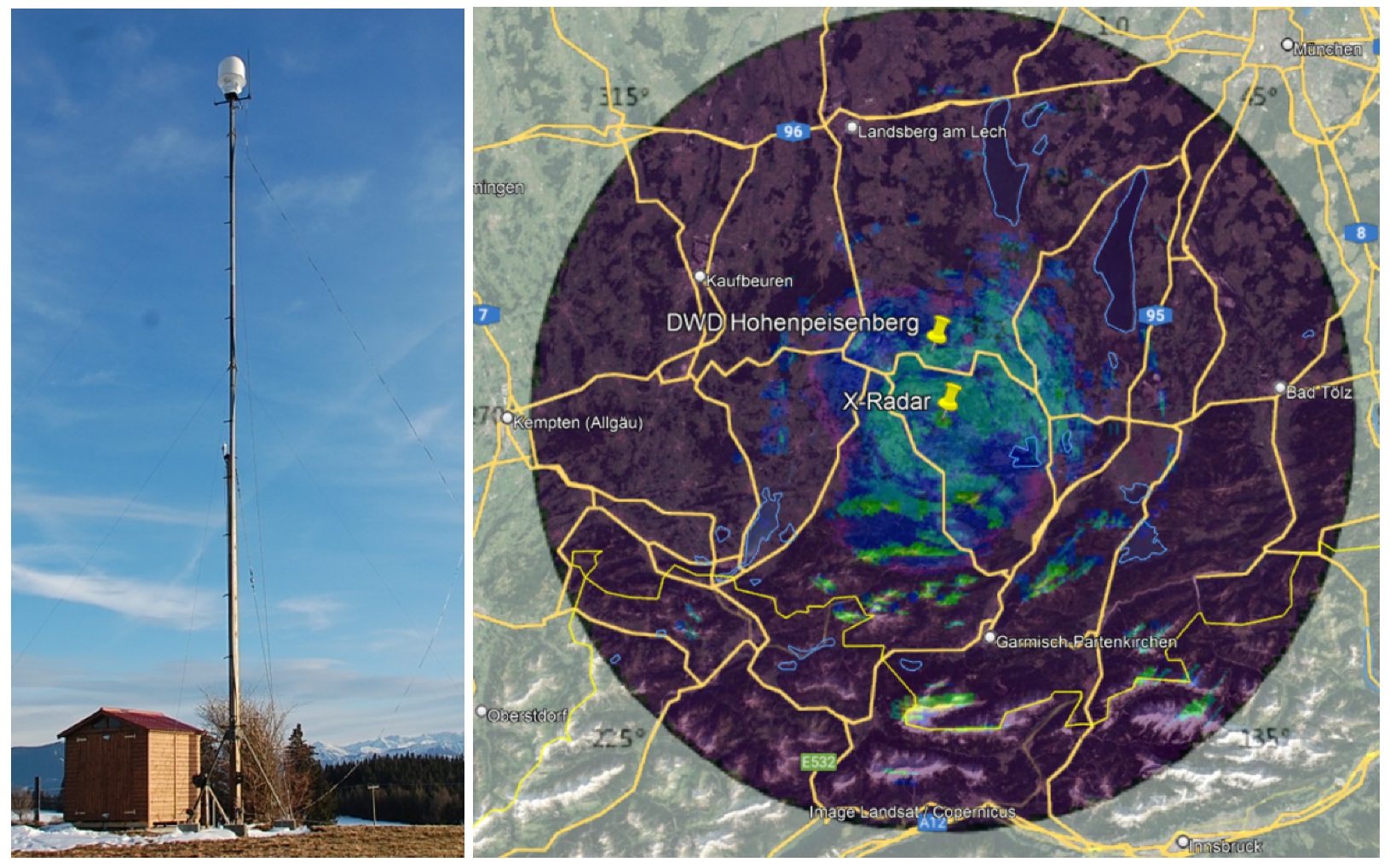
Figure 1 shows the location and of the X-Band single polarization radar, positioned in Kirnberg (Geigersau farm, Weilheim-Schongau, Bavaria, Germany) at 950 m height (a.s.l.). In this feasibility study, only the DWD station nearby the radar at the Hohenpeissenberg has been used for validation.

2.1. X-Band Radar

The raw radar data are measured with a maximum radius of 50 km around the radar position and with a horizontal resolution of 100 m. The radar acquired 12 scans of 360${}^{\circ }$ per minute. The five minute medians of the measured data are collected as a time series. More technical details about the radar are summarized in

Table 1. Technical details about the X-Band radar radar at Kirnberg (Geigersau farm, Weilheim-Schongau, Bavaria, Germany).

Antenna
Gain	37.5 dB
Azimuth Beam Width	2.5°
Elevation Beam Width	2.5°
Elevation Angle	3°
Rotation Rate	12 rpm (=12 rounds per slide)
Azimuth Accuracy	±0.5°
Weight (incl. Radome)	23.6 kg
Transmitter
Peak Power	25 kW
Frequency	9410 (±30 MHz)
Pulse Repetition Frequency	1500 Hz
Pulse Duration	500 ns
Pulse Length	75 m
Receiver
Bandwidth (1200 ns 500 ns)	2.5 MHz 7 MHz
Minimum Detectable Signal	−100 dBm
Dynamic Range	70 dB
Noise Figure	6 dB

.

2.2. Data Preprocessing

The raw data suffers from corrupted scans such as missing measured data, uncompleted scans, artifacts, or misaligned azimuth (wrong orientation). Empty scans are identified by a predefined threshold for minimum signal level (60 dBZ). Uncompleted scans are identified by wrong number of scanned azimuths, and the misaligned orientation of the scans is corrected by comparing the positions of distinct ground clutter (caused by mountains, e.g., the Mount Zugspitze) with a correct reference scan. These corrupted scans have been identified and removed.

In addition, the clutter effects, consisting of static clutter and speckles, have to be removed. The static clutter is caused by ground reflections around the radar (up to approximately 15 km radius) and by obstacles (mountains ranging from south east to south west). The clutter from the obstacles is very prominent with high reflectivities up to 50 dBZ. To remove the clutter due to obstacles, the relevant pixels of the scans are masked and the reflectivity is interpolated using the surrounding pixels. The ground clutter (e.g., around the DWD station Hohenpeissenberg) extends over a big area and cannot be handled as described above. Instead, we have calculated the mean reflectivity of this clutter using all clear sky scans of the relevant month and subtract this from the actual scan. The speckles are produced by moving objects (e.g., aeroplanes) and vary strongly in space and time. The extension of this phenomenon is limited to few pixels. The Gabella filter [21] has been used for masking and interpolation. The whole process of clutter removal has been extensively tested for the best parameter set of the filters (e.g., thresholds). The aim was to remove the clutter without introducing artifacts or removing small scale rain fields.

In the following, the raw measured Z has been used as input data, because there is no reliable way to correct for attenuation with a single polarization radar. For this study, data from May, June, and July 2015 and May, June, July, and September 2016 were chosen. The data were restricted to summer so that precipitation can be considered as rain with high probability. The temporal resolution of the meteorological observations is 10 min while the radar measures in 5 min intervals. Thus, two 5 min radar measurements were combined with the corresponding 10 min station observation so that uncertainties from upscaling were minimized. After removing missing or erroneous data, 26,554 data samples (10 min time resolution) were available.

To compare the performance of different models for different time resolution, hourly time series were generated by aggregating the raw data. In that case, 4268 data pairs could be used for the analyses.

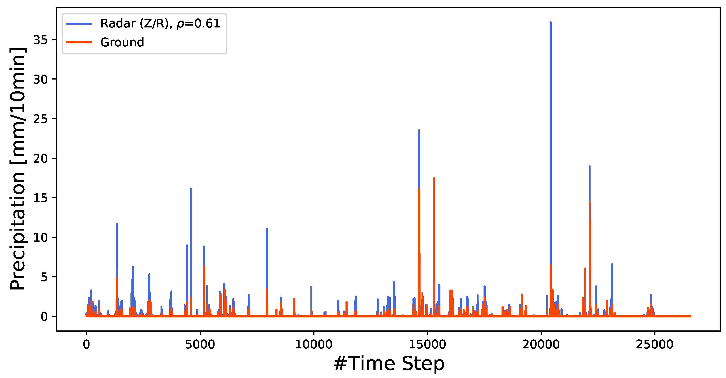
Figure 2 shows a comparison between observed precipitation and precipitation calculated from radar reflectivities by the standard Z–R relationship in 10-min resolution exemplarily for the station Hohenpeissenberg. The correlation between observed and radar based precipitation is 0.61. As only 3085 values are larger than 0 mm/10min, the observed mean is only 0.037 with a standard deviation of 0.30 mm/10min. It can be seen from Figure 2 that the position of rain events is well represented in the radar based data, while the absolute values tend to be overestimated.

This is also reflected in the scatter plot (Figure 3), where it can be seen that precipitation is systematically overestimated. Thus, the mean value of radar based precipitation is 0.08 mm/10 min leading to a bias of 0.03 mm/10 min.

2.3. Models

It is assumed that a Neural Network model is able to learn an appropriate non-linear transfer function that can reproduce the amount of precipitation, measured at the ground, from radar reflectivities and different meteorological input features.

To compare the performance of a transfer function based on a Neural Network directly with the empirical Z–R relationship, firstly a simple feed-forward Neural Network is set up which retrieves only radar reflectivities as input and is trained to reproduce rainfall at the ground as target.

Meta parameters of the ANN model include the number of hidden layers, the number of active neurons within each of them, as well as parameters that are connected to the learning procedure e.g., the learning rate. These meta parameters have to be adapted during training to optimize model performance.

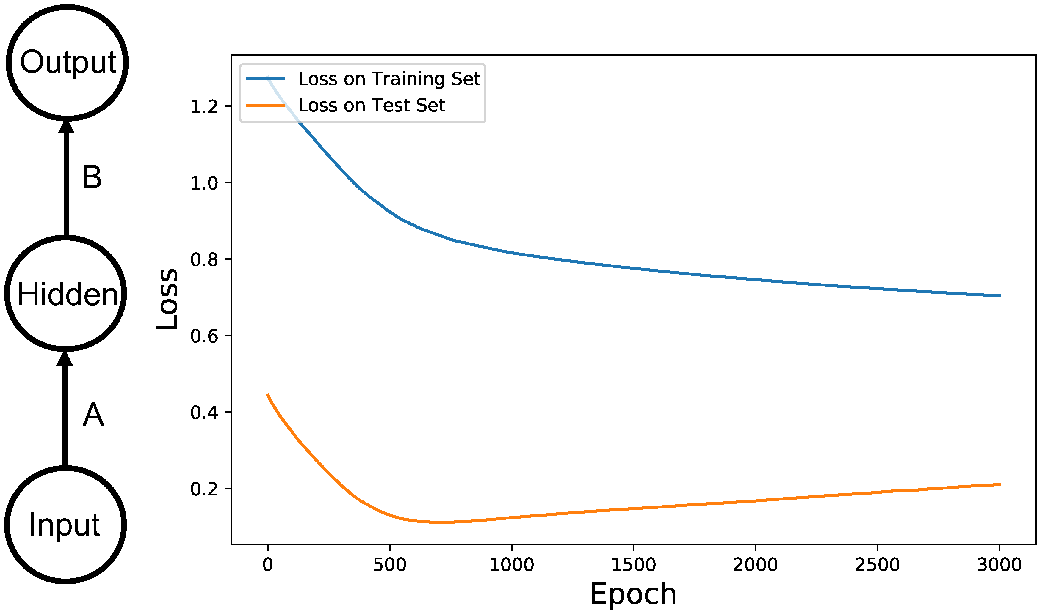
The Neural Network topology is kept simple with only one hidden layer (activation function tanh). The model topology is shown schematically in Figure 4 (left). The dimension of the input cluster depends on the size of the input feature space and is different for the individual settings, while the output cluster always has one dimension.

As a high-dimensional input space requires more complexity of the transfer function, the number of Neurons in the hidden layer is adapted with increasing input complexity and set to $(20+4·\mathsf{I}\mathsf{n}\mathsf{p}\mathsf{u}\mathsf{t}\mathsf{D}\mathsf{i}\mathsf{m})$. Thus, for only 1 input feature, the ANN has only 24 active Neurons in the hidden layer, while the number of Neurons increases to 44 when e.g., radar reflectivities with lags up to 5 are used as input features.

The number of trainable parameters (weights) in the connector matrices A and B is fully determined by the cluster dimensions. The number of free parameters in the respective transfer function $y_{out}=B(tanh(A\overrightarrow{x}))$ is thus increasing with an increased number of input features in $\overrightarrow{x}=(x_1,\dots ,x_k)$. A plot of the loss function during training of an exemplary model (hourly resolution, actual reflectivity only input) shows that the loss on the test set is decreasing continuously for the first epochs of training. However, after 600 epochs, it is starting to increase again while the training loss is still decreasing. This shows that the model tends to over-fit, i.e., it is learning too much detail from the training data while loosing its ability to generalize on unseen samples. To compensate for that effect, an early stopping procedure is implemented during training. The performance of the model on the test set is monitored during training and the learning is stopped as soon as the test error starts to rise again.

As the ranges of reflectivities and observed rainfall, as well as those of other meteorological variables, are substantially different, the data has to be standardized to a range of [−1;1] by a standard scaler $x_{i_{sc}}=\frac{x_i-\overline{x}}{{\sigma }_x}$ before feeding it to the Neural Network. The transformed data $x_{sc}$ then has mean $\overline{x_{sc}}=0$ and a standard deviation of ${\sigma }_{x_{sc}}=1$. This data range is also optimal for the $tanh$ activation function, as too large or too small values would be mapped to +1 or −1 while passing the hidden layer, leading to a loss of input information.

After standardization, the available data is split up into a training set (3400 for hourly and 21,000 values for 10-min time resolution), a test set (10% of the training data, randomly selected for each model run), and a fixed generalization set (850 and 5000 values). While the training and test set are presented during training and are used for model optimization as well as optimization of the different meta-parameters, the generalization set represents completely unseen data and is used for final performance estimation.

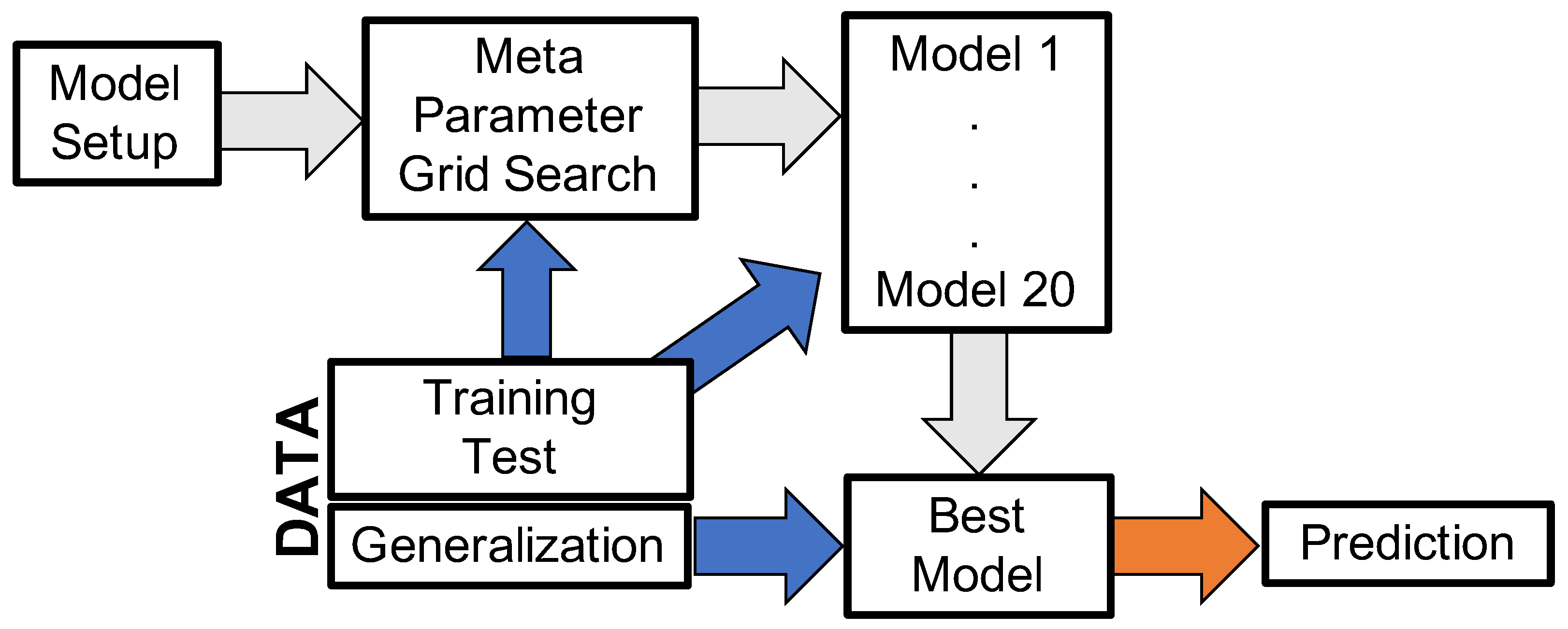
Figure 5 shows the workflow of model training and selection.

Based on the number of input features the respective number of hidden neurons is calculated and the first model is trained using stochastic gradient descent with momentum. The optimal meta-parameters of the training are found by a grid search. To avoid over-fitting, an early stopping procedure is applied during training with a maximum number of 3000 training epochs, which is large enough not to be reached before the loss on the test set increases. As the random initialization of model weights leads to slightly different performances in model recall, for all experiments an ensemble of models (20 ensemble members) is trained using the optimal set of meta-parameters. The best model is picked out based on the model loss evaluated on the test set.

2.4. Performance Measures

We use several statistical measures for the quantitative analysis of the modelling results. Besides the time series diagrams and scatter plots to visualize the performance, several standard performance measures are calculated, such as the bias, Pearson Correlation coefficient ($\rho$), the Root Mean Squared Error (RMSE), and the Nash–Sutcliffe Efficiency (NSE). Let $Q_i$ denote the $i=1,\cdots ,n$ observations, $\overline{Q}$ the mean of the observations, $Q_i^{\star }$ the modelled data, and $\overline{Q^{\star }}$ the mean of the modelled data. Then, the model bias that measures the difference between observed and modelled mean is defined as:

$$bias=\overline{Q^{\star }}-\overline{Q}.$$

(1)

The RMSE is a measure of the deviation between the two data sets, giving relatively more weight to larger differences. It is defined as:

$$\mathrm{RMSE}=\sqrt{\frac{1}{n}\sum _{i=1}^n{(Q_i^{\star }-Q_i)}^2}.$$

(2)

The Pearson Correlation coefficient ($\rho$) measures the strength and direction of the linear relationship between the modelled and observed data (perfect fit corresponds with $\rho =1$), and is calculated as follows:

$$\rho =\frac{{\sum }_{i=1}^n(Q_i^{\star }-\overline{Q^{\star }})·(Q_i-\overline{Q})}{\sqrt{{\sum }_{i=1}^n{(Q_i-\overline{Q})}^2}·\sqrt{{\sum }_{i=1}^n{(Q_i^{\star }-\overline{Q^{\star }})}^2}}.$$

(3)

The Nash–Sutcliffe Efficiency (NSE) is calculated as one minus the ratio of the error variance of the model divided by the variance of the observations. In case of a perfect model with an estimation error variance equal to zero, the resulting NSE value equals 1, whereas a model with an estimation error variance equal to the variance of the observations leads to an NSE of 0. The NSE is sensitive to extreme values and penalizes large outliers (perfect fit corresponds to NSE = 1). It is defined as:

$$\mathrm{NSE}=1-\frac{{\sum }_{i=1}^n{(Q_i^{\star }-Q_i)}^2}{{\sum }_{i=1}^n{(Q_i-\overline{Q})}^2}.$$

(4)

3. Results

In this section, the results of the different modelling approaches are compared. The shown results are calculated by evaluating the best model of the ensemble for the unseen data of the validation set.

3.1. Z–R vs. Simple Model

First, the influence of temporal resolution on the model performance is evaluated. For the comparison, we set up a basic Neural Network model where only the raw reflectivity at the actual time is used as input feature. The ANN is therefore trained to derive a non-linear transfer function similar to the empirical Z–R relationship that is able to translate raw reflectivities into precipitation.

3.1.1. Hourly Aggregation Level

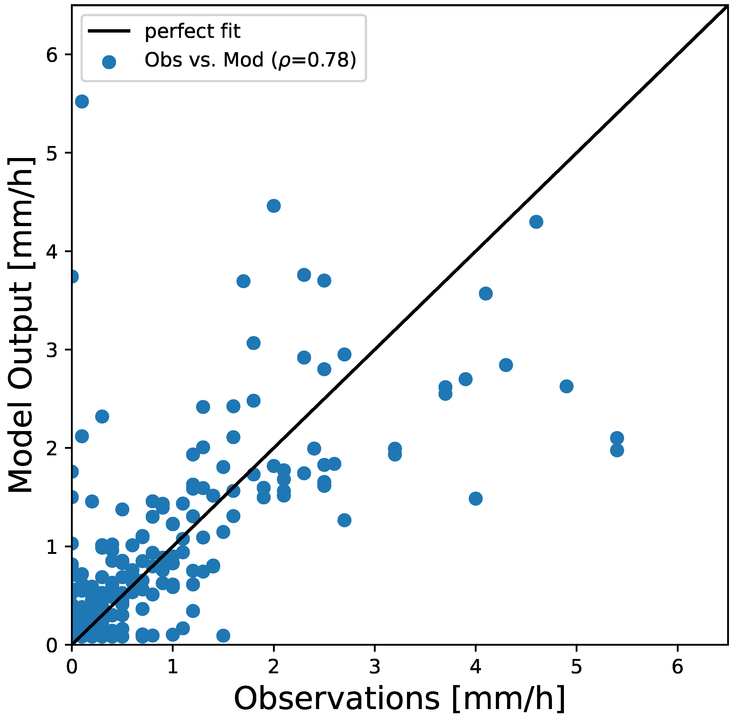
For the first calculations the data is aggregated to hourly time resolution. Figure 6 shows a scatter plot of modelled and observed precipitation for an hourly time resolution. The correlation between the two time series is 0.78 and thus slightly higher than for the standard Z–R relationship (0.67). It is also possible to reduce the systematic overestimation of precipitation amount as the bias is decreasing from 0.1 to 0.068.

3.1.2. The 10-min Time Resolution

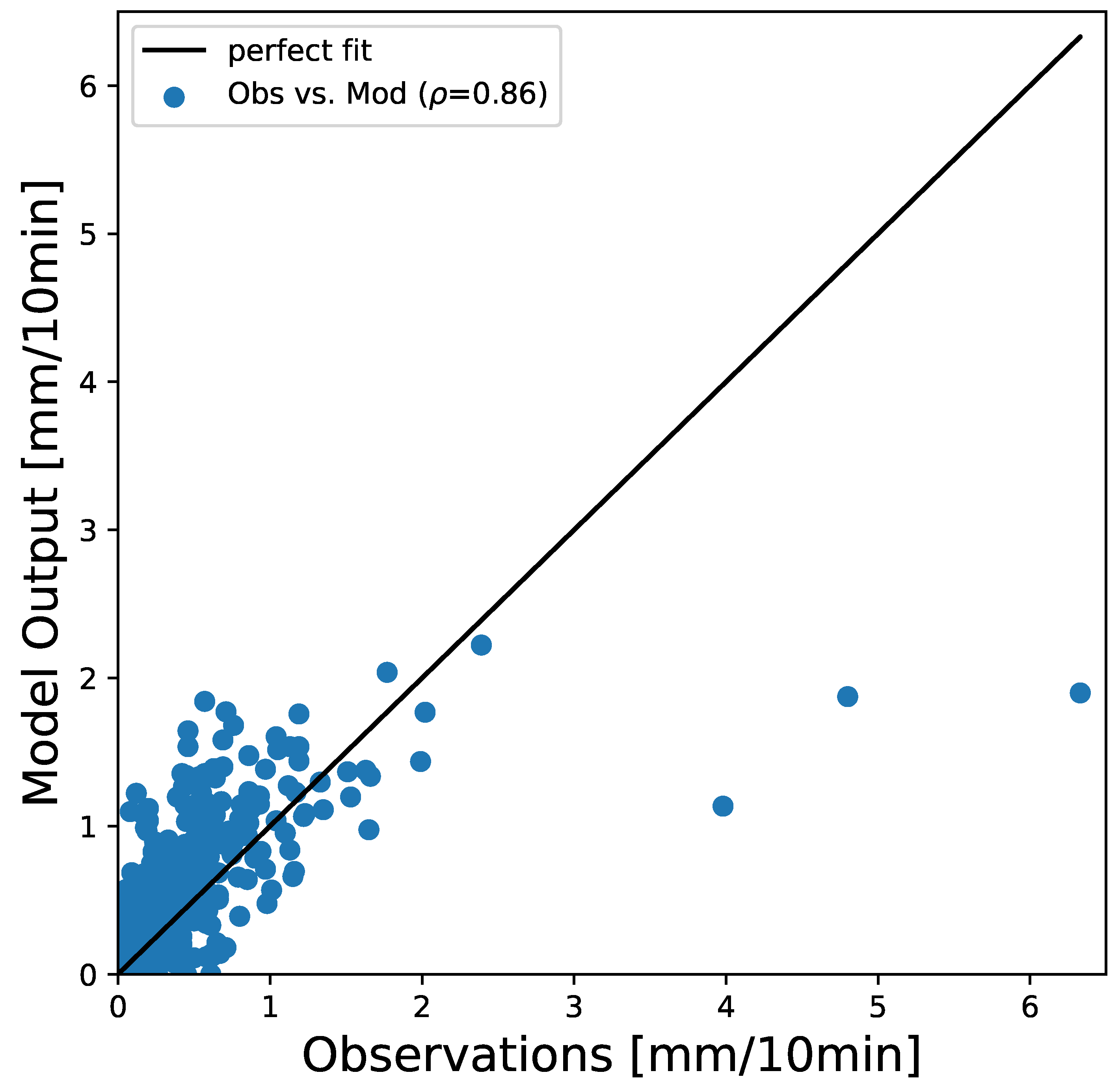
To estimate the influence of temporal resolution on model performance, the ANN is now trained with data in 10 min temporal resolution. As the radar reflectivities are available in 5 min time resolution, the Neural Network now retrieves two inputs, i.e., the two reflectivity measurements that are available within the respective 10 min interval. Figure 7 shows a scatter plot of modelled and observed precipitation on the validation set.

The correlation between modelled and observed precipitation is increased from 0.75 (Z–R relationship) to 0.86, while the bias is reduced from −0.08 to 0.01. Thus, the ANN model is tending to slightly overestimate the total amount of precipitation.

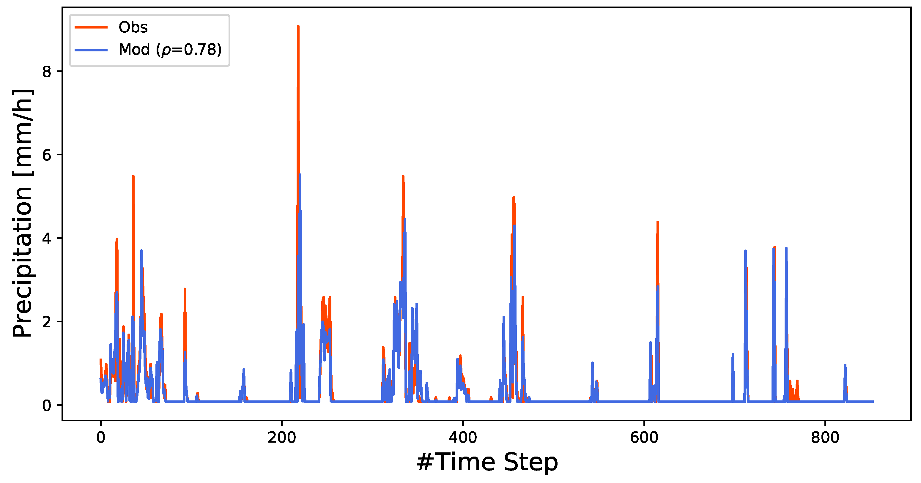
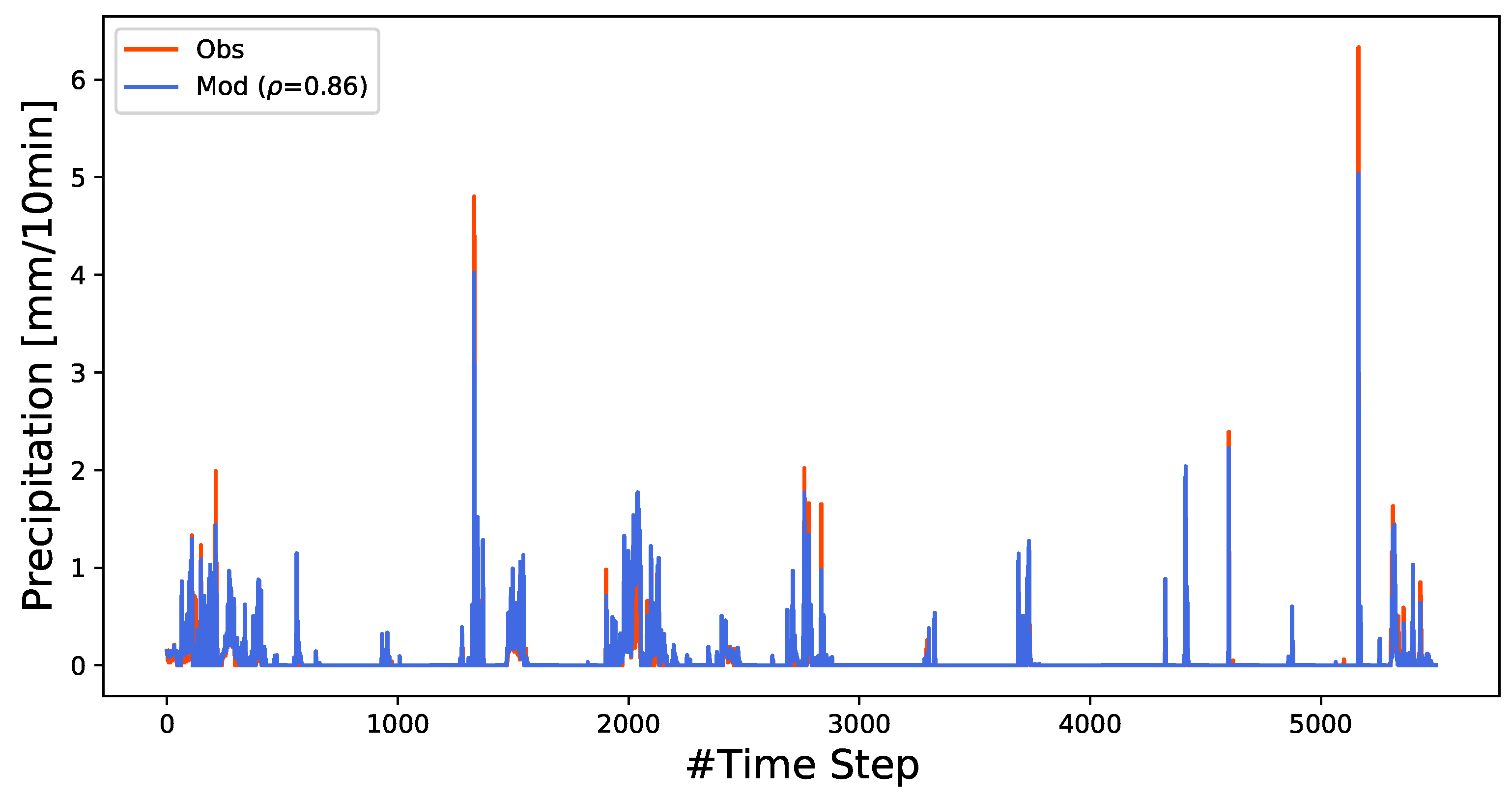
As the performance of the 10-min resolution model is slightly better than that for the hourly one, we keep the 10-min time resolution fixed for all other experiments. Plots of time series with modelled and observed precipitation for the two different time resolutions may be found in the Appendix (Figure A1 and Figure A2).

3.2. Time-Lagged Input-Reflectivity and Ground Precipitation

To further improve the model performance, additional input features are added. Time-lagged reflectivity measurements, as well as ground observations, are easily available and provide valuable information. Figure 8 shows the correlation matrix between precipitation from ground observations and radar-based values (Z–R relationship) with time lags. As expected, the correlation decreases from 0.61 (Lag 0) to 0.28 (Lags 4 and 5), indicating that radar observations with at least Lags 1 and 2 are relevant additional input features for subsequent modelling.

Table 2. Performance of Neural Network models where the dimension of the input feature space is stepwise increased by adding information from radar with different time lags.

	Lag 0	Lag 1	Lag 2	Lag 3	Lag 4	Lag 5
$\rho$	0.86	0.88	0.87	0.80	0.79	0.80
RMSE	0.11	0.10	0.09	0.12	0.13	0.12
bias	0.019	0.009	0.006	0.010	0.010	0.014
NSE	0.65	0.72	0.71	0.59	0.55	0.57

shows a comparison of model runs with increasing complexity of input feature space.

It can be seen that the correlation coefficient (0.88) and NSE (0.72) are highest for a model that retrieves reflectivities with Lag 0 and Lag 1 as input. The RMSE (0.10) and the bias (0.009) are only outperformed when Lag 2 information is additionally added (RMSE = 0.09 and bias = 0.006). It is also found that the addition of Lag 3 and Lag 4 does not further improve model quality, but indeed leads to decreased performance in terms of correlation, RMSE, and NSE, even in comparison with a simplistic modelling approach (Lag 0 input only).

Similar experiments with stepwise addition of lagged ground information lead to comparable results. The best model is found to be the one that uses actual reflectivity and Lags 1 to 4 of ground observations ($\rho$ = 0.87, RMSE = 0.08, bias = 0.005, and NSE = 0.75).

3.3. Meteorological Measurements as Input Features

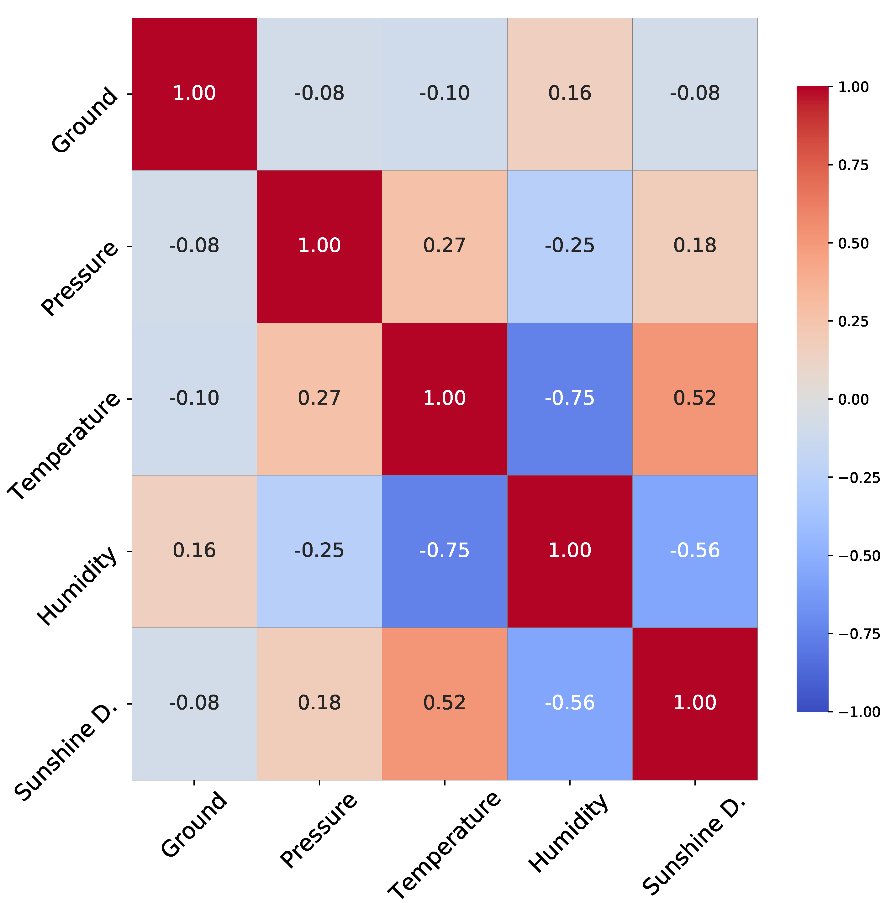
As it is not only precipitation at ground level which is available, but also other meteorological variables, we tested if model performance is improved by adding this information to the model input. Figure 9 shows the correlation between available meteorological variables and ground precipitation. It is found that humidity, followed by air temperature, has the highest correlation coefficient, with 0.16 and −0.1, respectively. As the correlation is found to be low in general, it is expected that these additional input features will only be able to contribute moderately to improved model performance.

Table 3. Performance of Neural Network models where the dimension of the input feature space of the Lag 0-Model is expanded by adding another meteorological variable, i.e., air pressure, air temperature, relative humidity, or sunshine duration.

	Lag 0	Air Pressure	Air Temp.	Relative Hum.	Sunshine Dur.
$\rho$	0.86	0.84	0.87	0.87	0.86
RMSE	0.11	0.11	0.11	0.09	0.09
bias	0.019	0.019	0.009	0.019	0.014
NSE	0.65	0.65	0.63	0.73	0.60

shows the performance of Neural Network models where air pressure, air temperature, relative humidity, or sunshine duration are added to the input feature space. It can be seen that, compared to the base model with only Lag 0 reflectivity as input, performance decreases slightly when air pressure is used. Nevertheless, a moderate improvement is observed for air temperature, relative humidity and sunshine duration.

3.4. Mixed Model—All Inputs versus Strong Inputs

As previous experiments show that model performance benefits from an expansion of input feature space, it is now tested if a model with all available input information outperforms those with reduced feature space. For the first calculation, a model is set up that uses time-lagged reflectivity and ground precipitation as well as all available meteo-variables. The second model uses only information that was found to improve performance i.e., time-lagged input with lags not larger than two, temperature, relative humidity and sunshine duration. Again, in both cases, a complete ensemble of models is trained and the best model is identified by evaluating the performance on the validation set.

Table 4. Performance of Neural Network with all available input features compared to best input only.

	Lag 0	All Inputs	Best Inputs
$\rho$	0.86	0.87	0.90
RMSE	0.11	0.10	0.08
bias	0.019	0.009	0.002
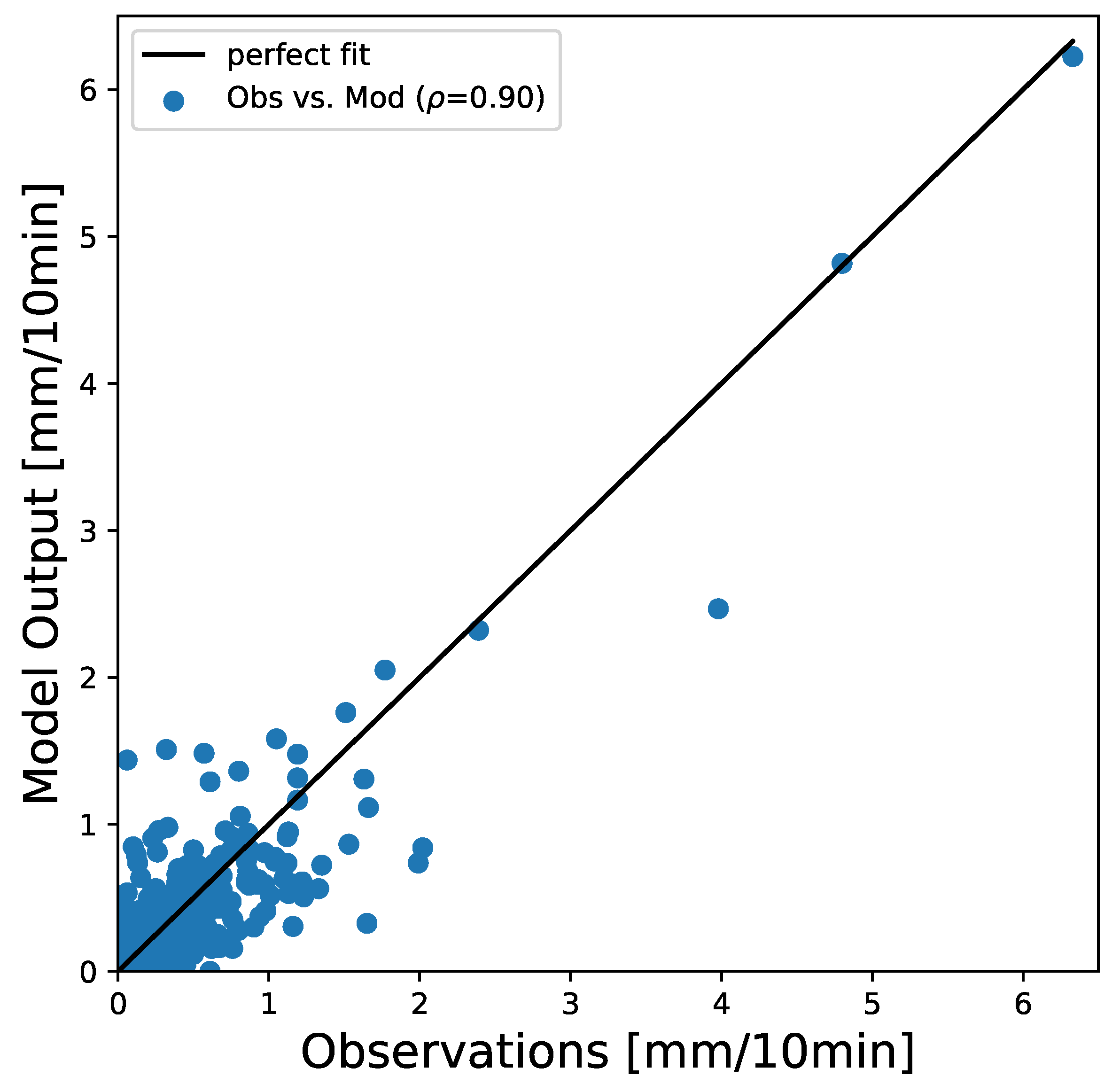
NSE	0.65	0.73	0.84

shows the results of best model runs. Compared to the basic model, a model with all input features shows a moderate improvement of performance with respect to all performance measures. However, a selection of only strong inputs leads to the best results within this study. Compared to the base model, the correlation between modelled and observed precipitation is increased from 0.86 to 0.90. The RMSE is reduced from 0.11 to 0.08, the bias decreases from 0.019 to 0.002, and the NSE increases from 0.65 to 0.84.

The improved model performance is also visible in the scatter plot shown in Figure 10.

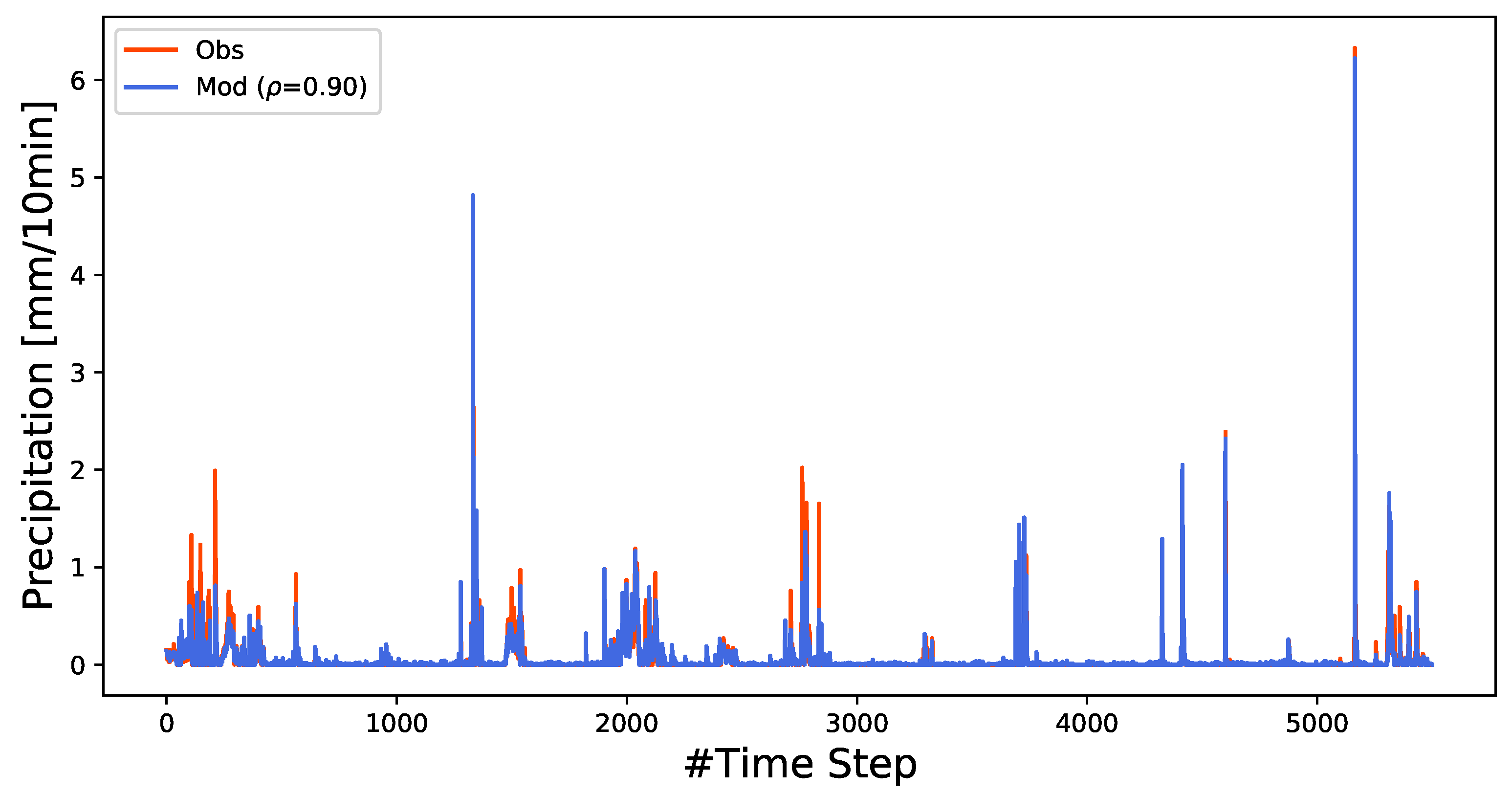
A plot of time series with modelled and observed precipitation for the best model configuration may be found in the Appendix A (Figure A3).

4. Discussion

It is shown that, already, simple ANNs are able to derive reasonable ground precipitation from raw reflectivities obtained from a X-band single polarization radar. This confirms previous studies that ANNs provide good nonparametric alternatives for traditional Z–R relationships in QPE (e.g., [8]). The performance and effectiveness of the QPE by using neural networks can be influenced by many factors such as the representativeness and sufficiency of the training data set, the generalization capability of the network to new data, season change, and location change (e.g., [8,22]). Furthermore, the type of the radar and settings have an impact. It is known that polarimetric radars provide more options and advantages for QPE than single-polarization radar (e.g., [3,23]).

In the case where only actual reflectivity is used as model input, the non-linear transfer function of the ANN model is structurally comparable to the empirical Z–R relationship. However, such models show an improved performance compared to that relationship in terms of all performance measures used in this study. The models perform similarly for time resolutions of 1 h and 10 min. In the first case, the correlation between modelled and observed precipitation increases to 0.78 compared to 0.67 with the Z–R relationship, while for 10-min resolution the model even reached a correlation coefficient of 0.86 (Z–R relationship: 0.75).

It could also be shown that additional input features are able to further improve model performance. In particular, time-lagged information from reflectivity, as well as the expansion of the input feature space with additional meteorological variables substantially improved the model quality. However, the input features have to be selected carefully. This is reflected by a direct comparison of a model with all available input to one with strong features only, that were identified by stepwise increasing model complexity. With a correlation of 0.9 and an NSE of 0.84, the latter outperformed all other models that were investigated.

Whenever radar reflectivities are used as input, preprocessing of the data e.g., clutter reduction, was completed before model training. This step is challenging and often requires expert knowledge (e.g., setting the best thresholds of filters for clutter reduction). Often, this step of preprocessing is even performed manually. It would therefore be a major advantage if it could be shown that ANNs are able to derive reasonable ground precipitation from reflectivity with a limited effort of manual preprocessing. Learning filters such as convolutional and pooling layers may provide a good alternative.

The ANN architecture, a three layer feed-forward net, is shown to perform well on the given data but may not be optimal as the underlying problem deals with time series modelling. For that, recurrent neural networks are known to outperform feedforward neural network models. It is thus promising to evaluate other ANN topologies for rainfall estimation. In addition, modelling of spatial representation of precipitation may lead to the necessity of including not only input feature vectors, but 2D input information. In that case, it is assumed that Convolutional Neural Networks are the most suitable model class, as they are able to respect for neighbourhood dependencies within the input feature maps (e.g., [3,14,17,18,19]).

5. Conclusions and Future Work

The recent study demonstrates that ANNs with carefully selected input features are outperforming the empirical Z–R relationship in deriving ground precipitation from measured radar reflectivities, as they are able to learn a non-linear transfer function from data.

Based on the results of this study, we answer the research questions as follows:

• Increasing the time resolution leads to improved model performance. The correlation coefficient between observed and modelled precipitation data is increased from 0.78 to 0.86, while the model bias is reduced from 0.07 to 0.01 for hourly and 10-min resolution, respectively.
• It is found that models that use reflectivity with time lags up to Lag 2 as input outperform those with actual information only. This is reflected by an increase in the correlation coefficient to 0.87 and reduced model bias of 0.006.
• A comprehensive predictor screening shows that meteorological variables can further improve the modelling results. It is found that air temperature and relative humidity provide the most valuable additional information to the model.

It is concluded that model performance is dependant on all three ingredients: time resolution, time lagged information, and additional meteorological input features. Taking all of these into account, the model performance can be optimized to a correlation of 0.9 and minimum model bias of 0.002 between observed and modelled precipitation data, even with a simple Neural network architecture.

However, the challenge is not only to derive reliable QPE for radar grids with station data, but also for those without. Thus future work has to address the open research question if it is possible to transfer the learned relationship between reflectivity and precipitation to locations in between. In doing so, it is necessary to restrict the input feature space to available variables, i.e., time lagged reflectivities and interpolated meteorological features such as pressure fields. Due to the discussed challenges with the preprocessing of the radar data, one of the main subjects of future research is how to derive improved precipitation fields in high spatio-temporal resolution with a limited effort on the preprocessing. As it could be shown that an evidence-based choice of predictor variables significantly improves model performance, it can be expected that approaches from deep learning also benefit from an extended input feature space. In this study, only one station is used for validation. More stations are required to analyse to what extent this approach can be transferred in space. In this context, the next step could also be to apply deep learning algorithms for spatial extension. Another issue is that the vertical displacement to the ground bound gauge causes a time delay between the reflectivity and the observed precipitation time series. It is shown that the introduction of lagged reflectivity values to the input feature space of the ANN is able to compensate this time delay at least to some extent. However, the effect is strongly coupled to general atmospherical conditions such as the prevalent wind direction and magnitude. Coupling reflectivity time lags to wind direction and wind speed, therefore, is assumed to further reduce time delays between modelled and observed precipitation time series.