Determination of River Hydromorphological Features in Low-Land Rivers from Aerial Imagery and Direct Measurements Using Machine Learning Algorithms

Abstract

Hydromorphology of rivers assessed through direct measurements is a time-consuming and relatively expensive procedure. The rapid development of unmanned aerial vehicles and machine learning (ML) technologies enables the usage of aerial images to determine hydromorphological units (HMUs) automatically. The application of various direct and indirect data sources and their combinations for the determination of river HMUs from aerial images was the main aim of this research. Aerial images with and without the Sobel filter, a layer of boulders identified using Yolov5x6, and a layer of direct measurements of depth and streamflow velocity were used as data sources. Three ML models were constructed for the cases if one, two, or three data sources were used. The ML models for HMU segmentation were constructed of MobileNetV2 pre-trained on ImageNet data for the feature extraction part and U-net for the segmentation part. The stratified K-fold cross-validation with five folds was carried out to evaluate the performance of the model due to the limited dataset. The analysis of the ML results showed that the measured metrics of segmentation using direct measurements were close to the ones of the model trained only on the combination of boulder layer and aerial images with the Sobel filter. The obtained results demonstrated the potential of the applied approach for the determination of HMUs only from the aerial images, and provided a basis for further development to increase its accuracy.

1. Introduction

The main goal of water protection is the good condition of all water bodies. The European Union (EU) Water Framework Directive [1] mandates that all water bodies must reach good conditions in all EU member states. Good conditions are understood as a well-functioning aquatic ecosystem that ensures suitable conditions for biodiversity to live. Poor biodiversity is most often caused by hydromorphological changes in the water body, by persistent pollution, or by a combination of both. In the Water Framework Directive (WFD), hydrological regime, river continuity and morphological conditions were pointed out as the three main elements of hydromorphological river quality.

In the WFD, hydromorphology is referred to as the “hydromorphological quality elements which support biological quality elements”. Based on this, we can conclude that hydromorphology can be defined as a field of study that includes measurements made to monitor changes in water volume and flow, riverbed, substrate, riverbank, riparian zone, aquatic and riparian habitats, and it can also be used to determine ecological status. Accordingly, the hydromorphology is a multidisciplinary research field that studies and evaluates the physical, hydrological, and morphological characteristics of water bodies and the processes that determine these characteristics.

The biggest hydromorphological impacts on water bodies are related to the impact of anthropogenic activity and the operation of hydropower plants [2]. The installation of hydropower plants and hydrotechnical structures of other purposes in riverbeds change the hydrological regime of rivers and damage the integrity of rivers. The operation of such hydrotechnical structures has a significant impact on aquatic organisms and sediment transport, and simultaneously on the ecological conditions of rivers [3,4]. Disruption of river integrity can significantly affect the ecological status of both upstream and downstream river sections.

Numerous hydromorphological assessment methods were developed and applied in the past few decades in different countries. One of these methods is the physical (in-field) assessment of hydromorphological features. This method is still current and useful because it does not require special knowledge; however, the understanding of basic principles and processes is necessary. Depending on local conditions, this method was practiced in Austria, France, Finland, Italy, Portugal, and Slovenia [5,6]. Field measurements for hydromorphological unit data were used in earlier studies for Latvian [7,8], German [9,10], Polish [11] and Greek [12,13] rivers as well. A review of assessment methods for river hydromorphology was done by Belletti et al. [14], identifying their main strengths, limitations, and the need for further improvements. Thus, these regular surveys for river hydromorphology have certain limitations themselves; conducting them takes long time and requires considerable manpower as well [10,15]. Hydromorphological data collection can be facilitated by combining a laser rangefinder, geographic information system (GIS) and remote sensing methods [16,17,18]. The use and convenience of these remote sensing methods for hydromorphological monitoring were discussed by Entwisle et al. [19], Beißler and Hack [20], and Hou et al. [21]. Comparison between field surveys and remote sensing approaches, as well as growing accessibility of remote sensing data, suggest the development of new methods for hydromorphological assessments of rivers to reduce the number of field surveys [22].

The rapid development of unmanned aerial vehicles (UAVs) and advancements in the miniaturization of instruments and data systems have led to the increasing use of this technology in the environmental science community. The use of UAV data has also become easier and more widespread because electronics were greatly improved over the past decade, making the process user-friendly and at a lower cost [23]. The purpose of some studies was to analyze changes in riverbed morphology using UAV aerial imagery, where interaction of the researcher is still necessary for analysis of the photogrammetric results [24,25,26]. Similarly, other authors identified photogrammetric methodologies based on high-resolution UAV aerial imagery as the suitable tool of choice for reliable hydromorphological assessment [27,28], which were valid in specific environmental situations [29]. Modern UAVs (multi-rotor) could collect images of a 1 km-long and 200 m-wide meandering river [30]. There are also many studies where both UAVs and automated data processing were used for the identification of hydromorphological features in rivers with improved image quality by capturing high-resolution photography [31,32]. For example, the UAV and artificial neural networks (ANN)-based framework for the automated recognition of hydromorphological features demonstrates a level of accuracy of up to 81% in the classification of some features [31].

Rivers’ hydromorphology is determined not only by the morphological characteristics of the riverbed but also by the in-stream natural impediments. Boulders are one of the most widespread natural obstacles that cause the turbulence distribution across the river flow. The large-size boulders affect hydrodynamics and morphodynamics of the surrounding area [33]. The effects are especially highly expressed along both sides of the boulder where the acceleration of the flow is induced [34] and behind the boulders or their groups [35]. The latter area is described by the decelerated flow and emergence of the vortexes. The longitudinal impact of the boulders on the river flow is quantified by the decreased velocity up to one boulder’s diameter upstream and up to five boulders’ diameter downstream [35,36]. The mentioned flow distortions under the influence of boulders create unique microhabitats that are essential for the maintenance of biodiversity, since the different hydraulic patterns and pulsations are found and can change in spatial and temporal scales depending on the discharge situation [37]. Moreover, natural obstacles play an important role in the spawning migratory patterns and detailed monitoring of them by applying drones could expand not only the understanding of how to manage the barriers [38], but also how to involve those data for hydromorphological assessment.

The artificial intelligence (AI) algorithms allow one to automatically process a large amount of data, extract hidden patterns, and establish relationships between variables. AI includes a subset called machine learning (ML) which consists of algorithms based on learning from data without explicit programming [39]. The ML algorithms are applied in various river research topics, namely the environment, ecology, hydrology, sanitation, human health, and socioeconomics [39]. The aerial or satellite images are used as input to classify fluvial scenes in a pixel level to water, sediments and vegetation [40], to identify hydromorphological units [32], to monitor aquatic vegetation [41], and to predict bathymetry [42] and other issues. The chosen AI methods and input pre-processing approach depend on the problem, data collection possibilities and costs, as well as computational resources.

The variety of colors of the river, irregular boundaries and lack of structure make it difficult to identify the river region from the aerial image with RGB channels. Thus, hyperspectral [43] or near infrared [44,45] bands in the images are used for the remote sensing analysis of river. The input aerial image is modified by transforming it to the different color space [31,32], or extending the number of channels in aerial images by generating additional bands of information. The features extracted from the 2D orthomosaic maps and 3D digital elevation model (DEM) were added to the RGB image as supporting layers, therefore used as an input to classification model to detect and map fluvial forms, such as gravel accumulation, bank erosion, and others [30]. Supplementing the input with the supporting layers resulted in higher accuracy of the model. The satellite image and DEM were used to extract geomorphic variables, such as active channel width, slope gradient, and others, which were used in river scene segmentation with support vector machine (SVM) and random forest (RF) models [46]. The SVM and RF algorithms were also applied in multilevel ML classification of riverscape morphological units and in in-stream mesohabitats [45]. The unsupervised learning approach to group pixels on their reflectance properties in combination with the supervised learning model of ANN was applied to automatically identify river hydromorphological features from aerial images [31]. The two-phase convolutional neural network (CNN) classification was used to segment aerial RGB images of fluvial scenes to water, sediment, green vegetation, senescent vegetation, and paved roads, in combination with multilayer perceptron (MLP) [40]. Using this approach demonstrated that a relatively small amount of labelled data is needed for model training. The fuzzy CNN model trained on UAV-derived labels was proposed to classify fluvial scenes in aerial images as a cost-effective approach to monitor vegetation growth and investigate geomorphology. The connected component segmentation, Bayesian likelihood classification, and central line analysis were used to detect and map a stretch of river in the UAV images with RGB and near infrared bands [44].

Existing studies in Lithuania are not concentrated on the usage of UAVs in the assessment of hydromorphological features. There are some studies which used satellite data, but they focused more on the determination of snow characteristics [47], river ice detection [48] or biophysical classification of Lithuanian lakes [49]. The deficiency of the studies on the hydromorphological assessment applying remote sensing and automated ML techniques was found in the study area and a similar geographical zone. The properties of relatively slow streamflow of low-land rivers create new underestimated challenges for the evaluation of hydromorphology. Accordingly, it motivates the development of new approaches that would allow the delineation of the target hydromorphological units (HMUs) with acceptable accuracy and the lowest amount of human resources. Based on the listed insights, the main goal of this research was to evaluate various combinations of data sources collected thorugh direct and indirect measurements for the determination of river HMUs only from aerial images.

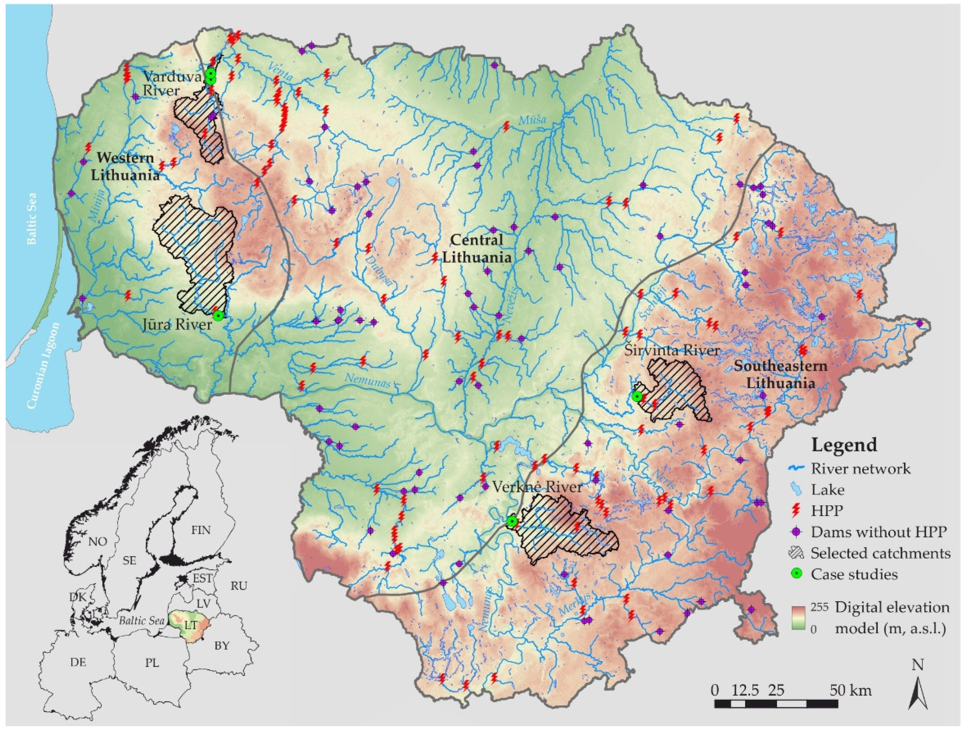
2. Study Area and Methods

Lithuania is a county in Eastern Europe near the Baltic Sea which covers an area of about 65,300 km². Under the Köppen climate classification, it has a humid continental climate. Thanks to its hydroclimatic conditions, the study area consists of a dense river network, since evaporation is less than the precipitation amount in the yearly balance. Accordingly, the area consists of around 4400 rivers longer than 3 km and an average density of 1.18 km/km² [50]. Lithuanian rivers are classified as low-land rivers because the average river slope rarely reaches a 1 m/km longitudinal gradient. Consequently, these rivers are usually distinguished by the even flow. Despite the dominating low gradients, there are many river sites where the slope increases and forms a diversity of river hydromorphology. Those sites did not remain unnoticed and the best river segments were used for dam-building purposes. Thus, around 102 hydropower plants (HPPs) and more than 1200 dams without HPPs have been built on Lithuanian rivers. These hydrotechnical structures highly affect the most valuable river stretches from a hydromorphological point of view. Therefore, four river catchments (Verknė, Širvinta, Jūra and Varduva rivers) affected by HPP activity were selected for this research (Figure 1). Case study river sites consisted of stretches downstream Jundeliškiai HPP on Verknė River, Širvinta HPP on Širvinta River, Balskai HPP on Jūra River, and Renavas and Vadagiai HPPs on Varduva River.

The research consisted of several main blocks that covered: (i) collection of ground truth data during the field surveys; (ii) processing of input data for ML model; (iii) simulation of ML model including its creation, training, and validation; and (iv) interpretation of the results (Figure 2). Each of the listed blocks had its individual subdividing, which, together with the detailed scheme of ML model, is described in the following sections.

2.1. Direct Measurements of Hydraulic Parameters and HMU Mapping

The survey of river hydromorphology consisted of discharge measurements in the studied river stretches, determination and mapping of HMUs at certain water discharge situation, and measurements of riverbed depths and streamflow velocities in delineated HMUs. Straight river segments without surface vegetation, boulders, and wood debris were selected for discharge measurements. The streamflow velocity in the selected cross-sectional profiles was measured using Valeport 801 Electromagnetic Flowmeters. The cross-section of the river was divided every 1 m, and streamflow velocity measurements were made at 0.2, 0.6 and 0.8 of the depth at each point.

The HMUs types, such as GLIDE, POOL, RIFFLE and RAPID, were identified in the studied river sites (Figure 3). The classification of HMUs was determined considering the riverbed morphology and hydraulic properties described in [51,52]. GLIDE is characterized by a low local slope and has a regular longitudinal bed profile, with a smooth or sometimes slightly rippled water surface due to low turbulence. POOL unit is characterized by topographic depression of the riverbed with a relatively slow flow velocity. The main difference between GLIDE and POOL is that the riverbed is not parallel to the water surface. RIFFLE is distinguished by a relatively shallow and fast flow and uniform sediments of riverbed armoring. These fractions rarely protrude out of the flow. RAPID is defined as a river channel unit that is mainly formed by boulders with a relatively steep riverbed. Such conditions create uneven flow with high turbulence zones around the stable boulders [51].

The mapping of boundaries of selected HMUs was performed using GeoMax Zenith 40 GNSS GPS (GeoMax AG, Widnau, Switzerland) receiver and X-PAD Ultimate Survey software (GeoMax AG, Widnau, Switzerland). The riverbed depths and streamflow velocities were measured in the identified HMUs. The mentioned parameters were measured at at least 10 points per delineated HMU polygon. All spatial data collected during the field surveys were processed and systematized using ArcGIS 10.5.

2.2. Aerial Mapping with UAV

The aerial imagery of the selected case studies area was collected using a DJI Phantom 4 Pro RTK UAV (DJI, Shenzhen, China). Firstly, five ground control points were placed on the site of the selected river stretch (four in the corners and one in the center) and their precise coordinates were measured with a GeoMax Zenith 40 GNSS GPS receiver. Photography was done automatically using a flight mission in native DJI software. The flight mission was conducted at a height of 35 m above the ground for getting the original ∼1–2 cm² per pixel (px) resolution with an overlap of 80%.

The post-processing of the collected data (generation of orthomosaic maps) was done using Pix4Dmapper (Pix4D S.A., Prilly, Switzerland) photogrammetry software. First, the point cloud of each river stretch was created based on images from UAV. In the second step, the point cloud and corresponding photographs were tied to ground control points for georeferencing and assigned a specific coordinate system. The final orthomosaic of the study area was created based on the georeferenced point cloud.

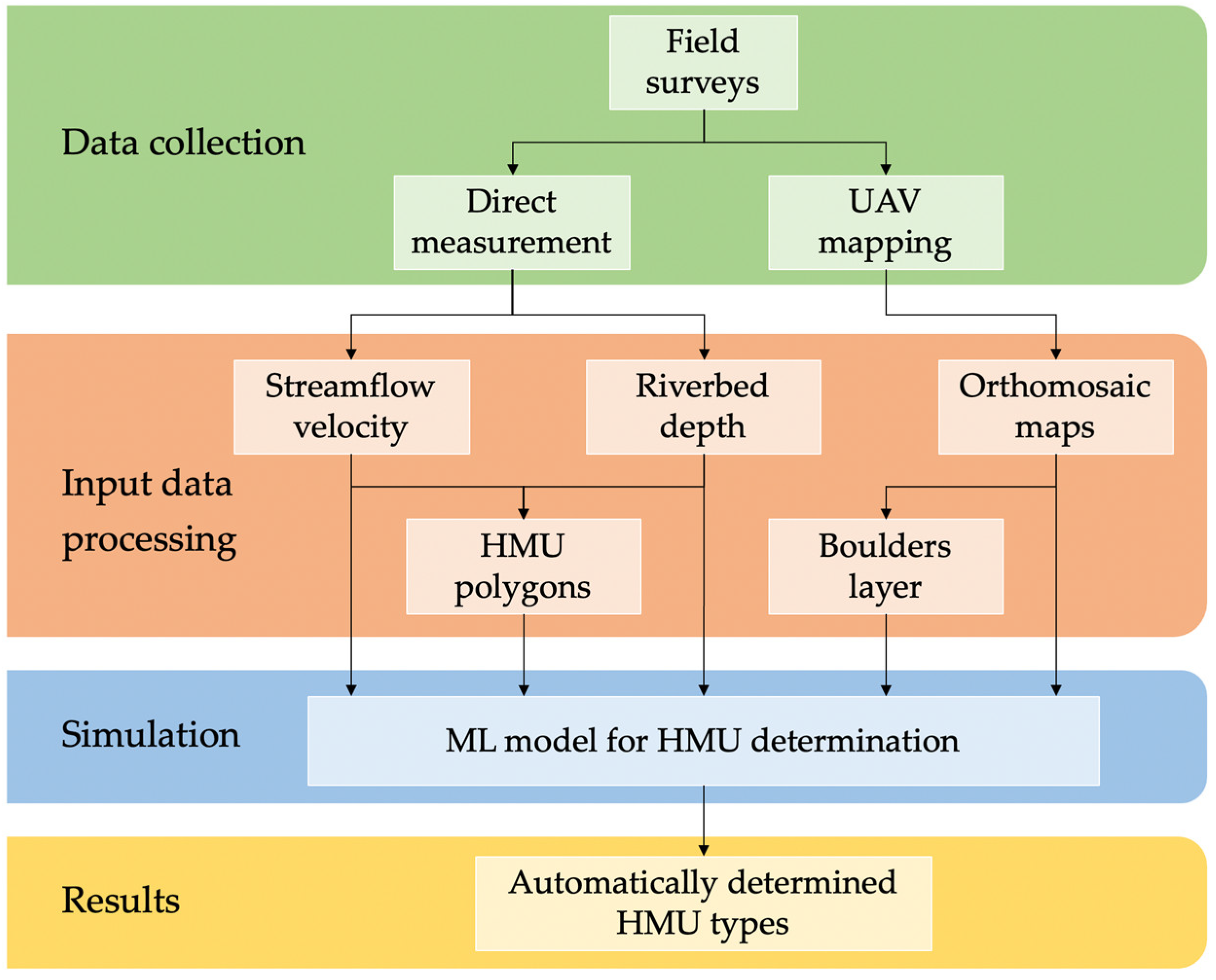
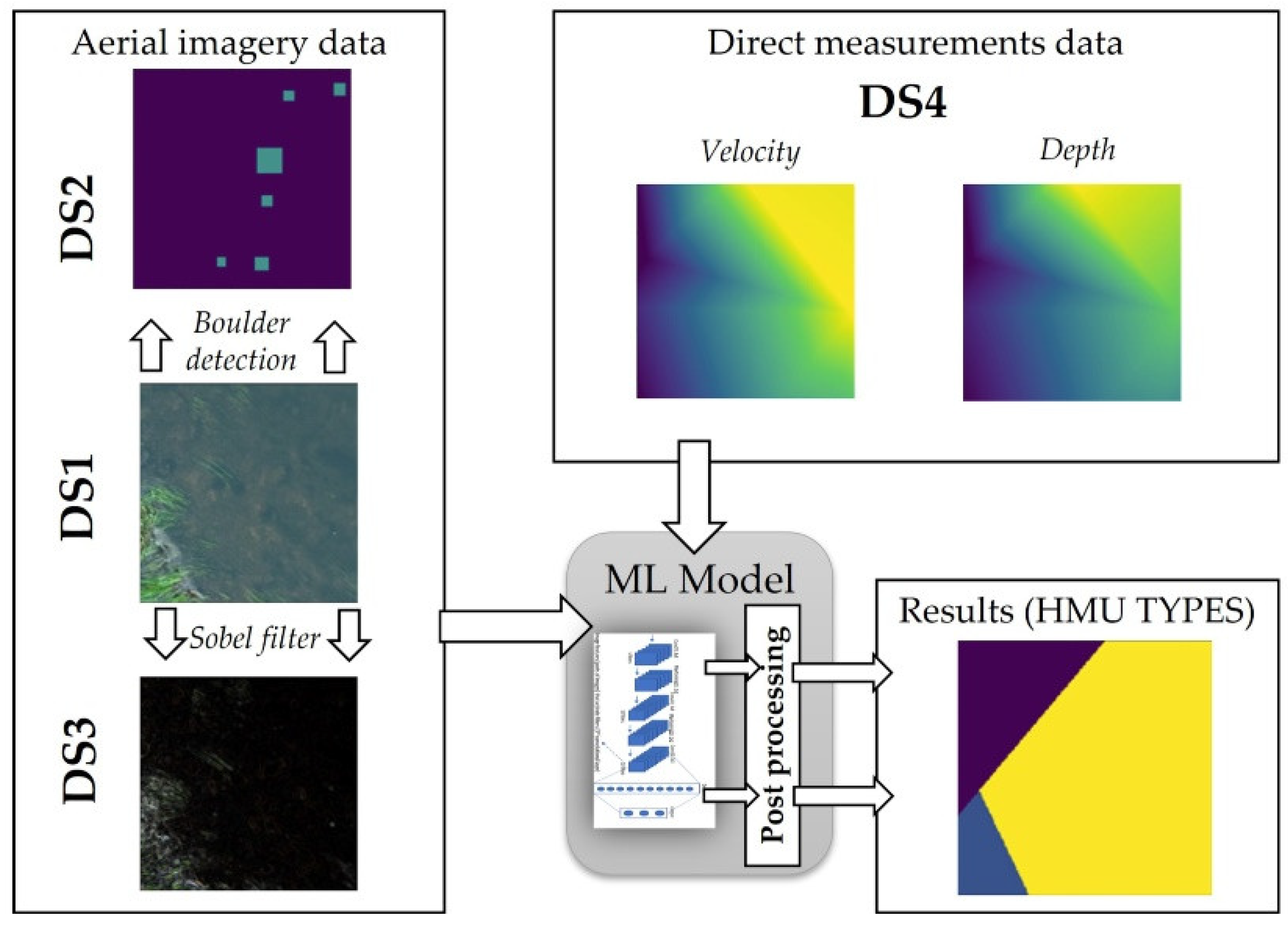
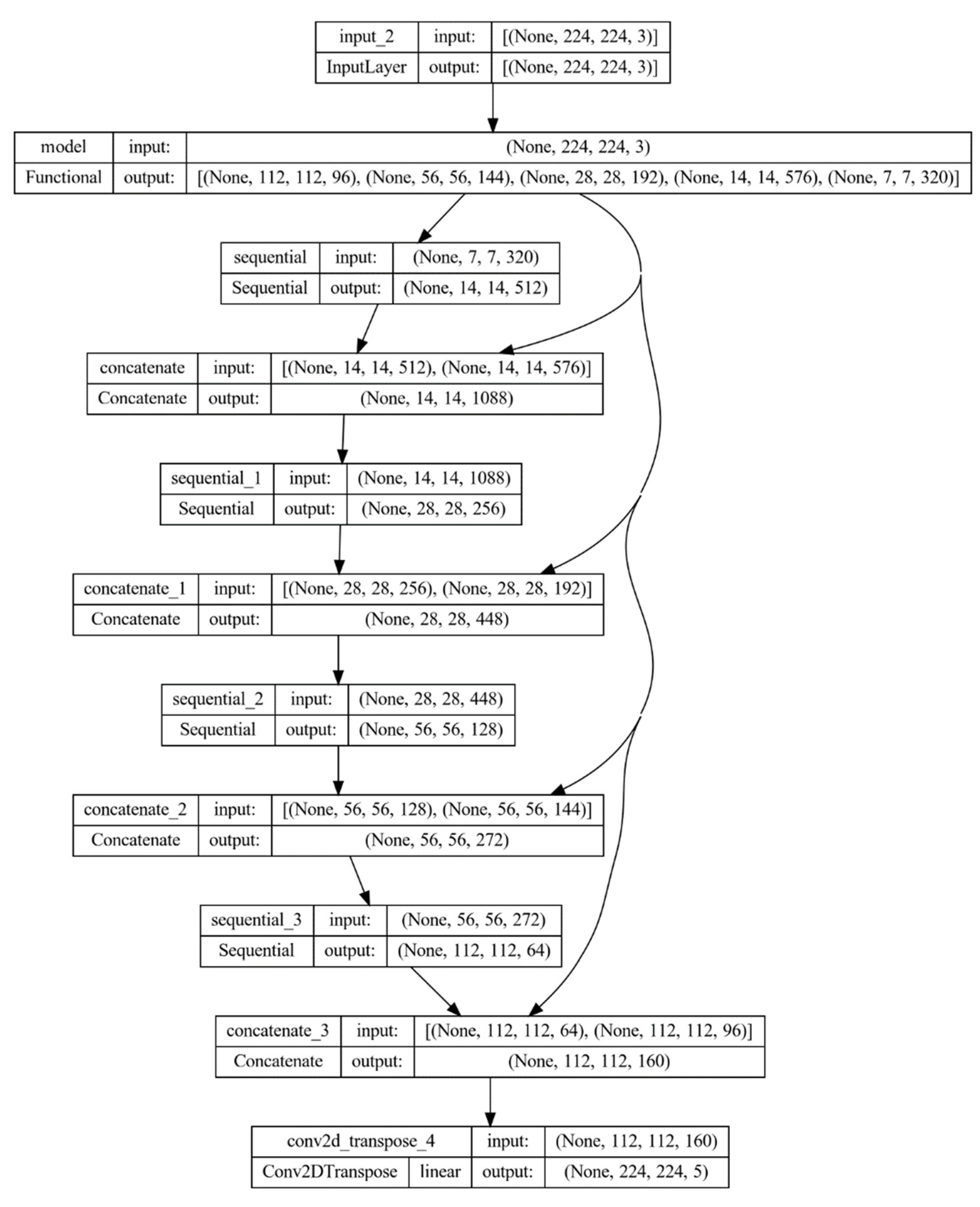
2.3. Automatic Detection of Boulders and HMU Determination from Aerial Imagery and Direct Measurements Data

In this study, the automatic detection of boulders and river segmentation to HMU types from the collected aerial images, their decomposition layers, and direct measurements data were performed. For the ground truth data, the experts mapped the bounding boxes of boulders and labelled HMU types for the range of rivers under the investigation.

Boulders can be the cause of streamflow turbulence or roughness of the river surface, which are the characteristic features of RIFFLE or RAPID HMU types. Thus, the number of boulders and their geospatial positions can help to determine the HMU type. The automatically detected boulders under and above the water surface may be used as an additional channel to the initial input data from aerial images for the river segmentation models. This channel contains the derived features and may, therefore, require less data for the training models. Other image decomposition techniques and direct measurements data such as streamflow velocities and riverbed depths may be added to the model in same way as the detected boulders. In this study, the analysis on how the accuracy of the ML model to determine HMU depended on different data sources and their combination for selected models was performed. In addition to RGB orthomosaic images (data source 1, DS1), the interpolated data of depth and velocities (data source 2, DS2), layer of detected boulders under and above water surface (data source 3, DS3), and results of Sobel filter applied on RGB orthomosaic images were used (data source 4, DS4).

Manual boulder labelling is a time-consuming process. Thus, the layer that represents boulders (DS3) should be created automatically without manual labelling. To create DS3 layer, an additional Yolov5x6-based model for object detection problem has been implemented with training dataset, which contained bounding boxes of the boulders under and above water mapped by the experts. To avoid usage of the same geospatial area for model training and evaluating its results, different models have been constructed in a K-fold cross validation procedure. After selecting the model architecture with the best performance, final DS3 layer was created for the images that were not used in training. The results of the boulder detection problem were used as one of the input features in the analysis of the HMU segmentation problem.

In this study, the analysis of HMU determination results by the means of accuracy was performed for the models trained with various input combinations. The cases of input data combinations were considered using only direct measurement data, only aerial images, and a combination of direct measurement data, aerial images and the output applying the Sobel filter or boulder detection to them. After training the model, the post-processing step was performed to reduce the output noisiness. In this step, the final decision of the HMU type of the pixel was made by taking the mode of the predicted HMU types in the square environment centered on the analyzed pixel. A generalized scheme of the applied data sources, ML model for segmentation, and output is provided in Figure 4. The structure of the ML model is described below.

The ten generated scenarios with combinations of different data sources are provided in

Table 1. Scenarios of models with combinations of input data sources (DS).

Scenario No.	Aerial Imagery Data	Direct Measurements Data	Label
1	-	DS4	depth-vel
2	DS3	-	photo-only (Sobel filter is ON)
3	DS1	-	photo-only
4	DS1	DS4	depth-vel-photo
5	DS3	DS4	depth-vel-photo (Sobel filter is ON)
6	DS2	DS4	depth-vel-boulder
7	DS3 + DS2	-	photo-only-boulder (Sobel filter is ON)
8	DS1 + DS2	-	photo-only-boulder
9	DS3 + DS2	DS4	depth-vel-photo-boulder (Sobel filter is ON)
10	DS1 + DS2	DS4	depth-vel-photo-boulder

. Firstly, the models were trained on separate data sources, that is, the aerial images without any transformations (Scenario No. 3), the aerials images after application of Sobel filter (Scenario No. 2), and the maps of depths and velocities (Scenario No. 1). To meet the conventional number of channels, the blank channel was added with equal values for all the elements. Secondly, the combinations of two data sources were used. The direct measurement data was combined with aerial image data using aerial images directly (Scenario No. 4), aerial images with Sobel filter (Scenario No. 5), and boulder mask (Scenario No. 6). The boulder mask was used in combination with original aerial images (Scenario No. 7) and the ones with Sobel filter (Scenario No. 8). Finally, the direct measurement data and boulder mask were combined with either aerial images (Scenario No. 10) or aerial images with Sobel filter (Scenario No. 9). All data sources were presented in the form of an image with three channels. For the DS4, the depth and velocity were stored in different channels, leaving the third channel filled with zeros.

Using different data sources results in different number of channels in input and, therefore, different model architectures. The architectures of segmentation models of different input size are demonstrated in Appendix A (Figure A1, Figure A2 and Figure A3). Segmentation model network architecture consists of two parts. The first part is dedicated to feature extraction. MobileNetV2 [53] architecture has been chosen due to its small footprint and low resource requirements [54] compared to other models, such as ResNet [55]. The MobileNetV2 pre-trained on ImageNet dataset was used in this research. ImageNet is a large dataset and using the model pre-trained on it enables the extraction of a large variety of patterns [56]. The second part of the segmentation model was dedicated to the classification of the pixels. The U-net [57,58] model with MobileNetV2 for connecting into U-net was implemented. The U-net model has a unique feature to exploit context information from an image due to its architecture. It was performed by processing input in multiple contracting layers and then up-sampling results, thus creating the U shape of model. The direct connection (called skip connection) between the contracting and up-sampling layers enabled one to fill the gaps of information and exploit the broader context.

2.4. Validation and Analysis of Results

The dataset used in this research was limited because of the complicated and expensive data collection procedure. Thus, training the ML model and evaluating its performance became a complex task. In order to validate the model’s performance, stratified K-fold validation technique was used. Such an approach enabled the interpretation of the stability of the results even for this relatively small dataset. To avoid similar data in training and validation datasets, the data were grouped according to the river segments. Firstly, the central line of the river region was constructed using morphological skeletonization algorithm. Then, it was divided into K equal pieces, and river region divided into segments by a line perpendicular to the central line. The folds were composed by including one segment of each analyzed river region in each fold. Based on the problem (boulder detection or HMU segmentation), the final dataset has been prepared for each selected piece in the following way:

• Boulder detection problem—taking N random points from the area under investigation and crop squared images around it. If a warped image contained no boulders, it was dropped from the dataset. Standard data augmentation procedure from YOLOv5 has been used, where a mosaic of original and three random images was loaded in training procedure.
• HMU segmentation problem—to apply augmentation in dataset preparation phase (different data source for model training requires same data transformation), the dataset was formatted by sliding 240 × 240 px window with a vertical and horizontal stride of 80 px. Only the areas which have at least 50% of actual data (visible water area with mapped HMU types) were included in the final dataset. Then, rotation augmentation was applied with image rotated by the step of 60°, that is, angles equal to 0°, 60°, 120°, 180°, 240° and 300°. The final 240 × 240 image has been cropped after rotation of a twice-larger image to avoid cases with no-data at squared image corners.

Precision, recall, and mAP-50 (mean average precision with 50% threshold for the intersection over union) were selected as model performance metrics in boulder detection task and the sum of mean squared error, binary cross entropy, and cross entropy as training loss function. For HMU type segmentation, the mean intersection over union (mIoU) was used as metric and the cross entropy as training loss function.

3. Results

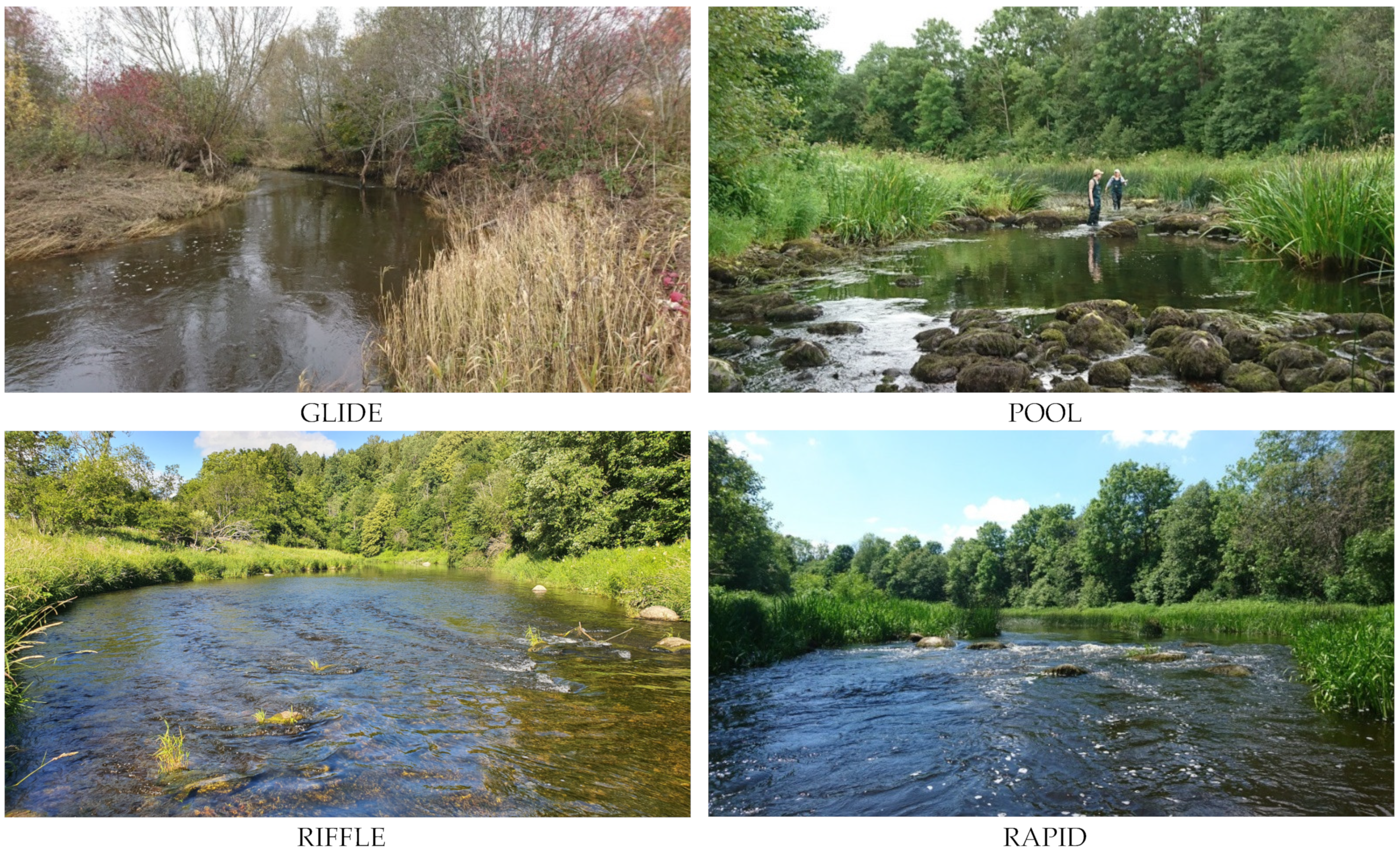
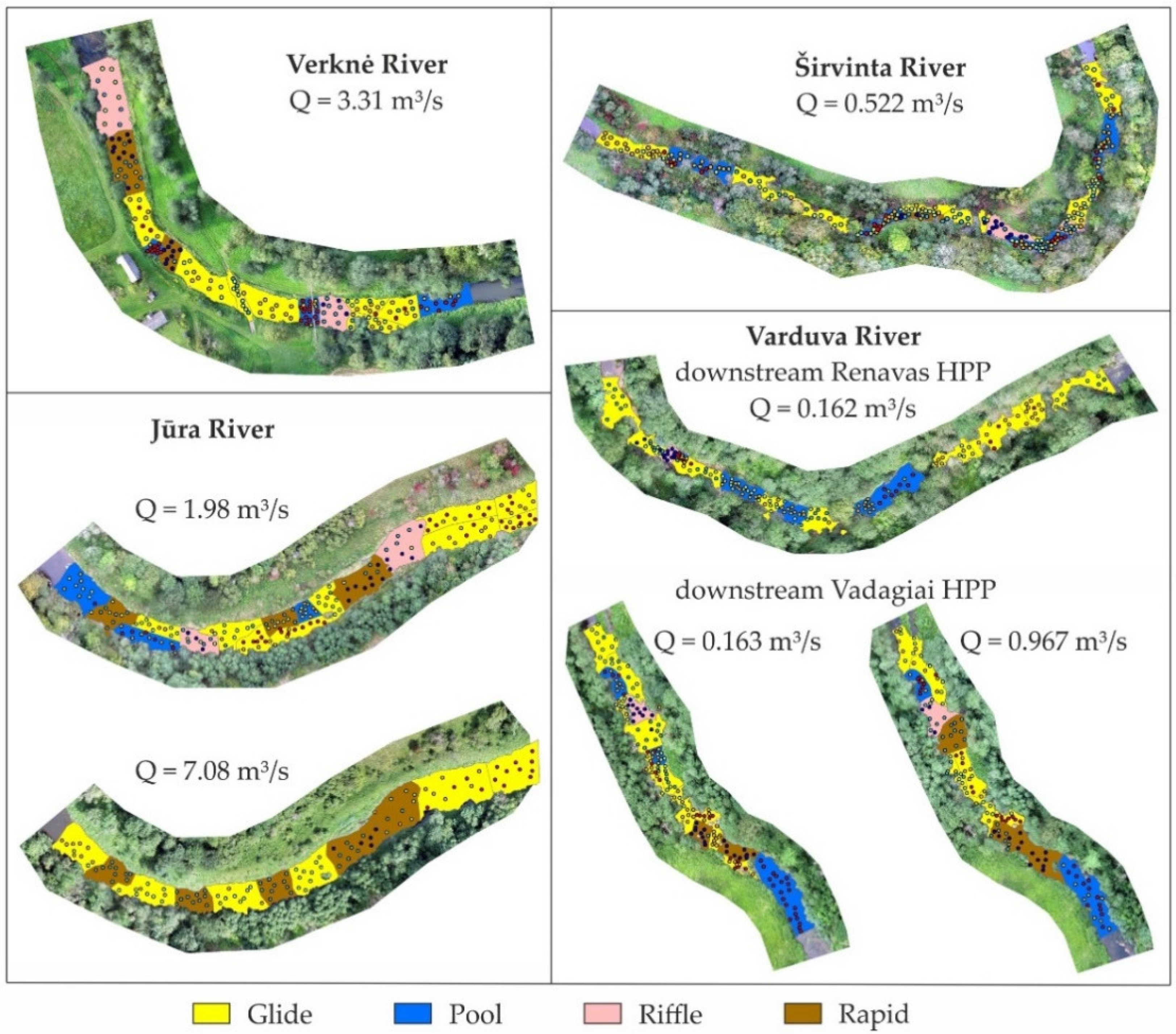
3.1. Distribution of the Hydromorphological Units

The mapping of HMUs and measurements of hydraulic parameters were done in four rivers at the discharge of the current situation (Figure 5). Only one discharge situation was measured in Verknė River downstream Jundeliškiai HPP and in Širvinta River downstream Širvinta HPP. For the Varduva River, two different river stretches downstream, Renavas HPP and Vadagiai HPP, were studied, since this river is affected by more than one HPP. The stretches downstream Vadagiai HPP and in Jūra River downstream Balskai HPP were distinguished by the two discharge situations measured, which highlighted the changes in hydromorphological units depending on the amount of water.

The length of mapped stretches varied from 164 m (Varduva River downstream Vadagiai HPP) up to 345 m (Širvinta River). The low-land rivers are characterized by monotonous streamflow and the absence of rapid changes. Therefore, the selected rivers segments were relatively abundant in diversity and quantity of hydromorphological units compared to the remaining stretches. In total, 16 to 21 HMUs were indicated per each case study segment; only at higher discharges below Balskai HPP (Jūra River) and Vadagiai HPP (Varduva River) did the quantity of HMUs reduce to 11 and 13, respectively. The most frequent HMU type across studied segments was GLIDE, which is common for the studied type of the rivers. The number of POOL polygons accounted for half of all GLIDE units, and they were distinguished by deeper properties. Units of RIFFLE and RAPID were identified less against the previous ones because only one to three units per stretch were found. Only one RIFFLE and no RAPID polygons were determined downstream of Renavas HPP. For the rivers with several discharges, the number of HMUs with more turbulent properties increased together with the increase in discharge.

The selection of HMUs type was done not only on the visual morphological indicators, but also based on the hydraulic features determined by the morphological changes. Information about the area and number of HMU polygons in each analyzed river stretch is provided in Appendix B (

Table A1. Area and numbers of HMU polygons at the analyzed river stretches.

River Discharge	Parameter	Analyzed River Stretch	Hydromorphological Unit
			GLIDE	POOL	RIFFLE	RAPID
Verknė 3.31 m3/s	Area (m2)	4632.1	2236.2	548.4	1104.2	743.2
	HMU polygons	16	7	4	2	3
Širvinta 0.522 m3/s	Area (m2)	2277.1	1288.4	695.4	216.7	76.5
	HMU polygons	21	10	8	2	1
Jūra 1.98 m3/s	Area (m2)	4851.8	2420.8	792.9	720.0	918.2
	HMU polygons	17	9	2	2	3
7.08 m3/s	Area (m2)	4848	3044.2	0.0	0.0	1803.8
	HMU polygons	11	6	0	0	5
Varduva
Renavas HPP 0.162 m3/s	Area (m2)	1733.2	1208.4	487.8	37.1	0.0
	HMU polygons	17	10	6	1	0
Vadagiai HPP 0.163 m3/s	Area (m2)	1576.9	872.1	453.6	81.0	170.3
	HMU polygons	17	10	4	1	2
0.967 m3/s	Area (m2)	1583.8	583.7	402.1	132.9	465.2
	HMU polygons	13	6	3	1	3

). The analysis of hydraulic parameters, such as depth of the riverbed and streamflow velocity, disclosed the main differences between determined hydromorphological units and similarities across the selected case studies (

Table 2. Average values of depth and streamflow velocity for different hydromorphological units in studied river stretches.

River Discharge	Parameter	Hydromorphological Unit
		GLIDE	POOL	RIFFLE	RAPID
Verknė 3.31 m3/s	Depth (m)	0.62	1.05	0.50	0.54
	Velocity (m/s)	0.422	0.260	0.609	0.757
Širvinta 0.522 m3/s	Depth (m)	0.38	0.73	0.25	0.35
	Velocity (m/s)	0.216	0.132	0.405	0.362
Jūra 1.98 m3/s	Depth (m)	0.54	0.85	0.35	0.44
	Velocity (m/s)	0.210	0.206	0.630	0.579
7.08 m3/s	Depth (m)	0.94	-	-	0.77
	Velocity (m/s)	0.540	-	-	0.873
Varduva
Renavas HPP 0.162 m3/s	Depth (m)	0.32	0.65	0.24	-
	Velocity (m/s)	0.144	0.078	0.385	-
Vadagiai HPP 0.163 m3/s	Depth (m)	0.29	0.68	0.17	0.21
	Velocity (m/s)	0.140	0.055	0.483	0.478
0.967 m3/s	Depth (m)	0.48	0.80	0.30	0.40
	Velocity (m/s)	0.235	0.141	0.540	0.577

). A relative change in depth and streamflow velocity, together with the water surface roughness due to the turbulence, were important parameters for HMU type indication in selected river stretches. The increasing discharge significantly affected depth and velocity values to the higher side. Depending on the measured discharge situation, GLIDE was described by the unit where average streamflow velocity fluctuated between 0.140 and 0.216 m/s, and average depth did not reach 0.48 m for the discharge situations of less than 1 m³/s. For higher discharges, the observed parameters increased up to 0.540 m/s in streamflow velocity and 0.94 m in river depth. The hydromorphological unit of POOL represented the relatively deepest places of the studied stretches because, despite the obtained discharges, the average depths ranged between 0.65 m and 1.05 m. The velocities were the smallest in POOLs and fluctuated between 0.055 and 0.141 m/s for small discharges and more than 0.200 m/s for higher discharges. Since RIFFLE and RAPID HMUs were quite similar in terms of streamflow velocity, the main difference between them was not only different patterns of surface roughness, but also the fact that RIFFLE was shallower than RAPID. Accordingly, the average depth of RIFFLE was around 0.17 and 0.30 m. Exclusively in Verknė River, the average depth was 0.50 m. Meanwhile RAPID units were 4 to 10 cm deeper on average comparing with the RIFFLEs.

3.2. Construction of Folds for Cross-Validation

The river features, light, and colors depend on the season the images were captured in. The stratified 5-fold validation was performed to include all examples of the analyzed rivers. In this research, the dataset was created for five river stretches (two of them were measured twice in different seasons and under noticeably different discharges). Thus, seven sets of aerial images and direct measurements were used. All seven river stretches were split into segments to prepare a dataset for 5-fold cross-validation. Skeletonization was performed to obtain the central river line for each analyzed river. Therefore, the river stretch was divided into five approximately equal parts (Figure 6) and all segments were assigned to different folds.

Different river segments were used in boulder detection and HMU segmentation models for training and validation. An overview of the generalized data of HMU areas and the number of boulders in each fold is provided in

Table 3. Composition of folds according to the mean of HMU area, number of HMU polygons and number of boulders.

Fold	Total Area (m2)	HMU by Type Area (Number of HMU Polygons)				Number of Boulders
		GLIDE	POOL	RIFFLE	RAPID	Under Water	Above Water
1	4117.1 (38)	2790.8 (22)	491.1 (7)	441.5 (3)	393.7 (6)	175	102
2	4279.3 (38)	2080.4 (20)	555.0 (9)	522.2 (3)	1121.6 (6)	531	457
3	4233.9 (23)	2298.8 (15)	439.5 (4)	495.2 (1)	1000.4 (3)	169	99
4	4621.6 (32)	3189.4 (16)	531.9 (9)	0.0 (0)	900.3 (7)	204	239
5	4244.4 (23)	1291.2 (8)	1361.3 (9)	832.9 (2)	759.1 (4)	389	200

.

3.3. Boulder Detection and Formation of DS3 Layers

The results of boulder detection were used as the pre-processed data in the model training. The object for investigation in the boulder detection task were two different classes labelled as boulders under water (BUW) and boulders above water (BAW). Object loss and precision curves for validation datasets during training are given in Figure 7. All folds in cross validation demonstrated the same trends during the training. The values of the loss function decreased as the epochs pass (Figure 7a). For all cases, the precision values did not change significantly after the 20th epoch (Figure 7b).

For validation datasets after training, the precision, recall, and mAP-50 metrics of both classes are shown in

Table 4. The precision, recall, and mAP-50 for the validation datasets.

Fold	Class	Objects	Precision	Recall	mAP-50
Train 2345-valid1	BAW	809	0.851	0.710	0.731
	BUW	1025	0.666	0.443	0.454
Train 1345-valid2	BAW	2453	0.766	0.797	0.805
	BUW	3091	0.578	0.339	0.361
Train 1245-valid3	BAW	664	0.798	0.664	0.719
	BUW	823	0.567	0.408	0.434
Train 1235-valid4	BAW	1670	0.669	0.764	0.773
	BUW	924	0.620	0.360	0.393
Train 1234-valid5	BAW	1673	0.798	0.515	0.579
	BUW	2485	0.734	0.404	0.462

. The results demonstrated that all metrics were better for BAW class in all datasets. Obviously, the detection of BUWs was more complicated because of the water layer above the boulder, vegetation, water surface roughness, and other features.

An example of the original image and boulder inference result is provided in Figure 8. The red and green bounding boxes represented the expected result, i.e., the manually labelled bounding boxes of BAW and BUW classes. The cross and diagonal patterns indicated the inference results of the BAW and BUW classes, respectively. The example in Figure 8 illustrated the tendency towards detection errors due to small boulders in the area of larger ones. Accordingly, the automatic detection was difficult, as well as labelling manually.

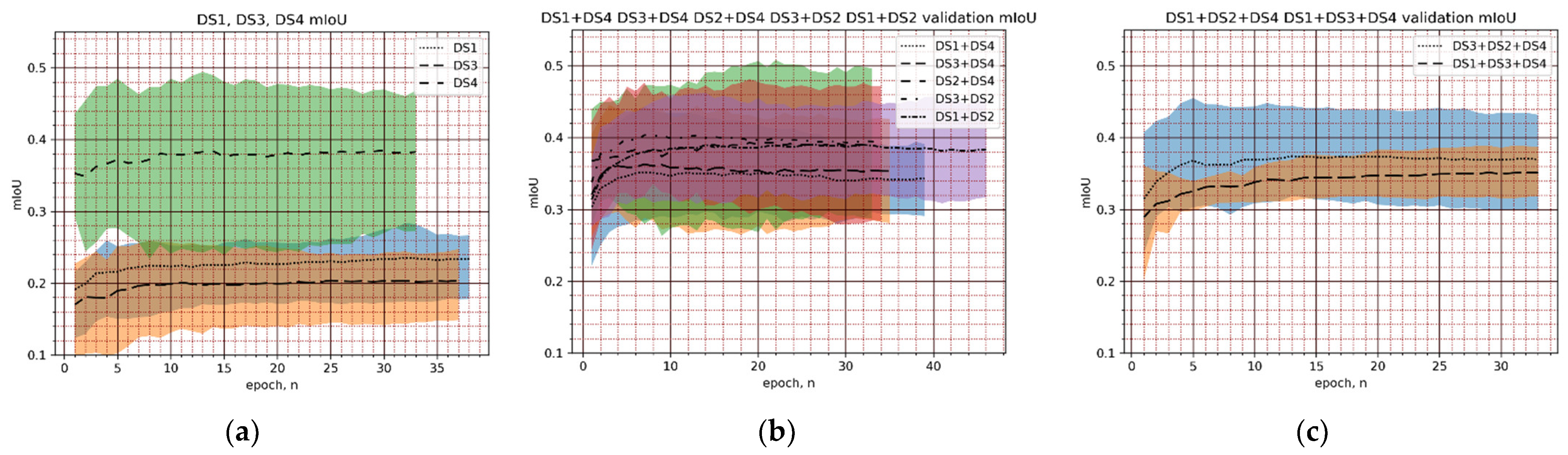
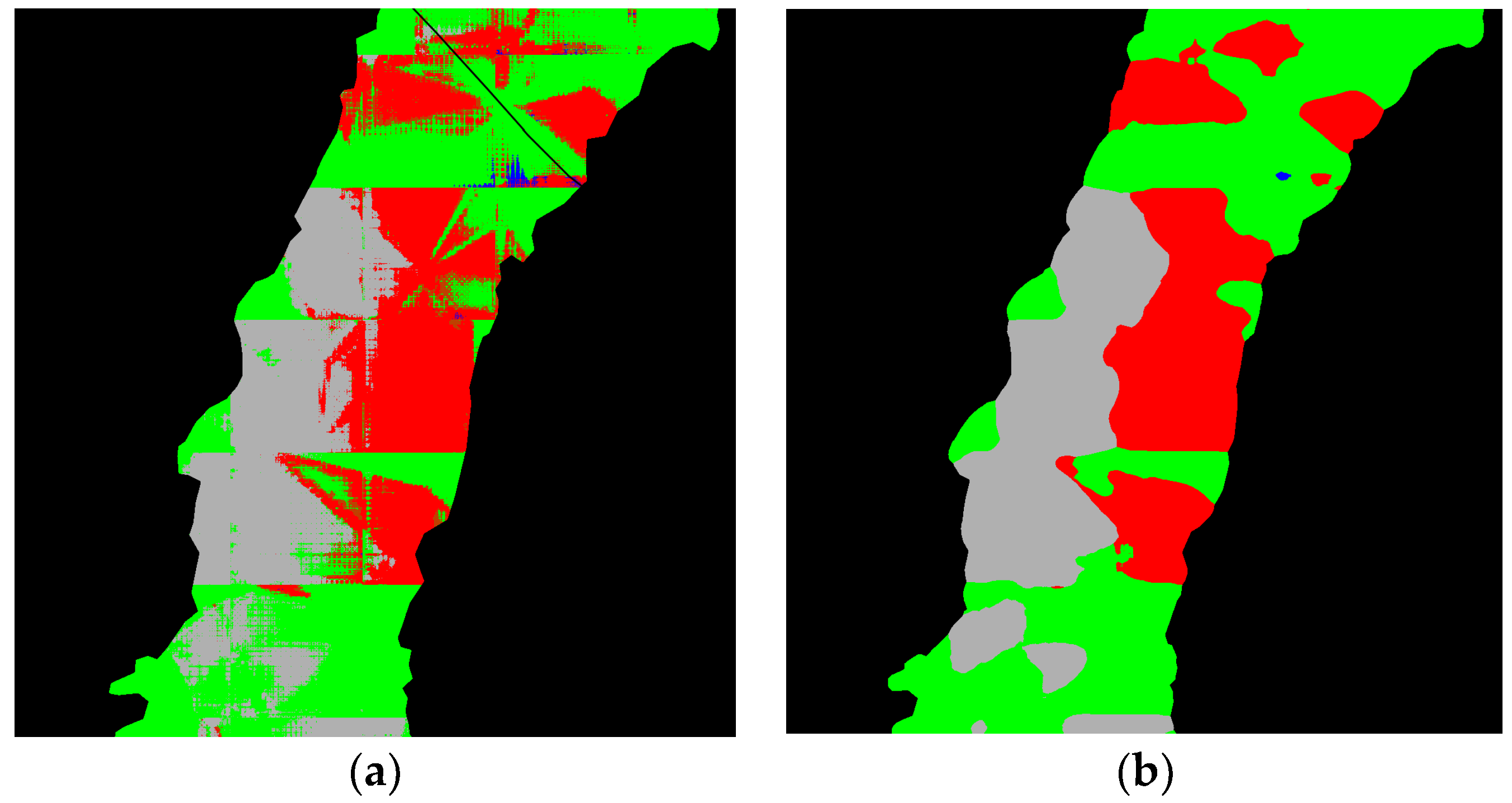
3.4. HMU Segmentation Results

K-fold cross-validation with five folds was performed to evaluate HMU segmentation results for all the generation scenarios of input data sources. The mIoU curves for the validation datasets are presented in Figure 9. The lines represented the mean value of mIoU in all the folds, whereas the area showed the minimum and maximum value of mIoU of the validation dataset in the folds. The performance results were provided from the perspective of the model architecture, i.e., the number of data sources used as the input. The calculations were done using TensorFlow software with NVIDIA A100 GPU. The training was set to 200 epochs, but with an early stopping condition of no improvement of validation mIoU in 32 epochs to prevent overfitting. In the results, the number of epochs was chosen with respect to the smallest value of epochs between the folds trained under the same scenario (combination of data sources). The results showed that the best performance was reached in approximately the 10 first epochs. The mIoU value did not change significantly for all the models. Analysis of the results showed that the best values of the measured metrics were given by the models, which were created using only DS4, combinations of DS2 with DS3, DS2 with DS4, and DS1 with DS2 (Figure 9a,b). Although averaged mIoU values of all scenarios did not exceed 0.4, the performance of scenarios with either DS1 or DS3 was significantly worse and did not exceed 0.3 (Figure 9a).

In the inference procedure, the ML model predicted the class of each pixel. In some cases, several pixels of one class were in the environment of the pixels which were assigned to another class. It should be noted that HMU polygons covered areas larger than several pixels. Thus, it was highly probable that such noisy cases represented the misclassified pixels. The post-processing step was added to the analysis. The final decision of the HMU type of the pixel was made by assigning the mode value of the inference results bounded by the 21 × 21 square centered on the analyzed pixel. The example of the inference results and results after post-processing are provided in Figure 10. Although the noise was reduced after the post-processing step, there were still small regions of the same class (blue region in Figure 10b). These small regions resulted in relatively low performance metrics.

To demonstrate the benefit of the post-processing step, the mIoU values for model output before and after the post-processing step are provided for all the scenarios in

Table 5. The mIoU value for the model output and post-processed model output.

Scenario No.	Data Sources	mIoU of Model Output	mIoU of Post Processed Model Output
1.	DS4	0.394	0.409
2.	DS3	0.243	0.254
3.	DS1	0.262	0.271
4.	DS1 + DS4	0.348	0.360
5.	DS3 + DS4	0.357	0.374
6.	DS2 + DS4	0.397	0.416
7.	DS3 + DS2	0.405	0.421
8.	DS1 + DS2	0.383	0.395
9.	DS3 + DS2 + DS4	0.382	0.405
10.	DS1 + DS2 + DS4	0.362	0.385

. The results showed that the mIoU values increased by approximately 3–6% after the post-processing step was applied. After the post-processing step, the mIoU values exceeded 0.4 for scenarios No. 1, 6, 7, and 9. Of these, only scenario No. 7 did not include direct measurement data (DS4). This case demonstrated that direct measurements were important features in HMU segmentation. However, similar segmentation metrics can also be achieved without the usage of direct measurement data.

4. Discussion

The evaluation of river HMUs [51,52] is a complex task that requires several components for comprehensive estimation. Local physico-geographical features create unique conditions that should be considered as well. In terms of this research, the dominant low-land rivers common across Lithuania and neighboring countries were selected. The ML applications to predict HMU types with aerial images involving direct measurement data were analyzed. Ten scenarios with different combinations of input data sources were applied to train ML models. The findings of the research revealed that the best performance was demonstrated by using only direct measurement data if one input source was considered, which is significantly worse than using direct measurements data when only aerial images were applied (with or without Sobel filter). The areal images of RGB channels, despite the good visual properties in expert evaluation, have their own limitations when tasks become more comprehensive and the training of ML algorithms steps into the development of object recognition approaches. To eliminate complex disturbances and accurately identify all available information from orthophoto images, multispectral images are used [59]. Then, a wider range of color bands is captured in comparison with the RGB scale and we have more information that helps accurately determine pattern differences that are invisible to the eye. For example, Wright et al. [60] were some of the first researchers to use multispectral images for mapping hydrogeomorphic units, and found out that it could be done at a fine scale.

Additionally, the scenarios with two input sources were tested and it was found that their performance metrics of all models were quite similar. However, using the boulder layer with either a layer of direct measurements or aerial images with a Sobel filter resulted in slightly higher (2–15%) mIoU value. This demonstrated that the direct measurements could be changed by the combination of boulder layer and aerial images with the Sobel filter. Accordingly, the remote measurements based on the analysis of aerial images enable one to determine the HMU types without measuring depth and velocity directly. The findings also showed that using three input sources consisting of boulder layer, direct measurements, and aerial images with or without the Sobel filter did not improve the HMU segmentation. However, the post-processing step led to 3–6% higher mIoU values compared to the mIoU values for the ML model inference results. These effects require further investigation, as it could be possible that the features in input layers contradicted each other and the higher number of input therefore resulted in worse performance. Some reasons could be related to the certain turbidity of low-land rivers. The selected rivers are characterized by relatively high turbidity depending on the hydrological conditions as a result of which optical properties of water transparency suffer. It is much easier to optically recognize the objects in “crystal clear” water [32], but based on the analysis of more than 80 media and high spatial resolution satellite images, the turbidity patterns of the Danube Delta waters [61] showed the complexity of such a task, and the application of MODIS satellite data for the long-term analysis of turbidity patterns confirmed that [62]. In addition, a certain layer of bottom sediments that changes in spatial and temporal scale characterizes the selected low-land rivers. The color spectrum of the bottom changes not only between seasons, but also during the course of the day due to different lighting and weather conditions. The purely visual recognition is reliant on good visibility, while the water quality becomes a critical limiting factor [28]. Therefore, the development of new or the improvement of current methods is essential for very turbid areas, with a special focus on the involvement of areal imagery with high spectral properties [25].

This research highlighted the importance of a higher number of data sources as input, which leads to a higher number of features and subsequently requires more data for training. A larger dataset of aerial images and direct measurements for various river stretches should be created to make the model more general. However, data collection is a complex procedure, and the aerial image data is sensitive to seasonal vegetation and weather conditions. It should also be noted that the ML model inference results are noisy and the noise reduction step should be included in the post-processing step.

5. Conclusions

The analysis of various scenarios of different inputs to construct an ML model that determines HMU types from the aerial images and direct measurement data was performed. The proposed approach was based on the supervised learning with the HMU types as labels determined by the experts. The results showed that models trained on the direct measurement data and on the combination of boulder layer and image demonstrated similar accuracy after applying the Sobel filter.

Two main directions were identified for future research. Firstly, the variety of inputs for the ML model can be expanded by using multi-spectral images or various methods for feature extraction and image decomposition. The second direction is based on the combination of ML model with aerial images as input and the validation of its results using physically based hydraulic models.

References

1. Council directive 2000/60/EC establishing a framework for Community action in the field of water policy. Off. J. 2001, L327, 1–73. Available online: https://eur-lex.europa.eu/legal-content/EN/TXT/?uri=CELEX:32000L0060 (accessed on 15 November 2022).
2. Cesoniene, L.; Dapkiene, M.; Punys, P. Assessment of the impact of small hydropower plants on the ecological status indicators ofwater bodies: A case study in lithuania. Water 2021, 13, 433. [Google Scholar] [CrossRef]
3. Gierszewski, P.J.; Habel, M.; Szmańda, J.; Luc, M. Evaluating effects of dam operation on flow regimes and riverbed adaptation to those changes. Sci. Total Environ. 2020, 710, 136202. [Google Scholar] [CrossRef] [PubMed]
4. Kiraga, M. Hydroelectric Power Plants and River Morphodynamic Processes. J. Ecol. Eng. 2021, 22, 163–178. [Google Scholar] [CrossRef]
5. Raven, P.J.; Holmes, N.T.H.; Charrier, P.; Dawson, F.H.; Naura, M.; Boon, P.J. Towards a harmonized approach for hydromorphological assessment of rivers in Europe: A qualitative comparison of three survey methods. Aquat. Conserv. Mar. Freshw. Ecosyst. 2002, 12, 405–424. [Google Scholar] [CrossRef]
6. Ferreira, J.; Pádua, J.; Hughes, S.J.; Cortes, R.M.; Varandas, S.; Holmes, N.; Raven, P. Adapting and adopting River Habitat Survey: Problems and solutions for fluvial hydromorphological assessment in Portugal. Limnetica 2011, 30, 263–272. [Google Scholar] [CrossRef]
7. Jēkabsone, J.; Uzule, L. Assessment of the hydromorphological quality of streams in the Venta River Basin district, Latvia. Est. J. Ecol. 2014, 63, 205–216. [Google Scholar] [CrossRef] [Green Version]
8. Jekabsone, J.; Abersons, K.; Kolcova, T.; Tirums, M. First steps in the ecological flow determining for Latvian rivers. Hydrol. Res. 2022, 53, 1063–1074. [Google Scholar] [CrossRef]
9. Meir, G.; Zumbroich, T.; Roehrig, J. Hydromorphological assessment as a tool for river basin management: The German field survey method. J. Nat. Resour. Dev. 2013, 3, 14–26. [Google Scholar] [CrossRef] [Green Version]
10. El Hourani, M.; Härtling, J.; Broll, G. Hydromorphological Assessment as a Tool for River Basin Management: Problems with the German Field Survey Method at the Transition of Two. Hydrology 2022, 9, 120. [Google Scholar] [CrossRef]
11. Wiatkowski, M.; Tomczyk, P. Comparative assessment of the hydromorphological status of the rivers Odra, Bystrzyca, and Ślȩza using the RHS, LAWA, QBR, and HEM methods above and below the hydropower plants. Water 2018, 10, 855. [Google Scholar] [CrossRef]
12. Stefanidis, K.; Latsiou, A.; Kouvarda, T.; Lampou, A.; Kalaitzakis, N.; Gritzalis, K.; Dimitriou, E. Disentangling the main components of hydromorphological modifications at reach scale in rivers of Greece. Hydrology 2020, 7, 22. [Google Scholar] [CrossRef] [Green Version]
13. Stefanidis, K.; Kouvarda, T.; Latsiou, A.; Papaioannou, G.; Gritzalis, K.; Dimitriou, E. A Comparative Evaluation of Hydromorphological Assessment Methods Applied in Rivers of Greece. Hydrology 2022, 9, 43. [Google Scholar] [CrossRef]
14. Belletti, B.; Rinaldi, M.; Buijse, A.D.; Gurnell, A.M.; Mosselman, E. A review of assessment methods for river hydromorphology. Environ. Earth Sci. 2015, 73, 2079–2100. [Google Scholar] [CrossRef]
15. Novakova, J.; Melcakova, I.; Svehlakova, H.; Marcakova, L.; Matejova, T.; Klimsa, L. Hydro morphological assessment of the Porubka river. In Proceedings of the 1st International Conference on Advances in Environmental Engineering (AEE 2017), Ostrava, Czech Republic, 28–30 November 2017; Volume 92, p. 012046. [Google Scholar] [CrossRef]
16. Bedla, D.; Halecki, W.; Król, K. Hydromorphological method and gis tools with a web application to assess a semi-natural urbanised river. J. Environ. Eng. Landsc. Manag. 2021, 29, 21–32. [Google Scholar] [CrossRef]
17. Koutrakis, E.T.; Triantafillidis, S.; Sapounidis, A.S.; Vezza, P.; Kamidis, N.; Sylaios, G.; Comoglio, C. Evaluation of ecological flows in highly regulated rivers using the mesohabitat approach: A case study on the Nestos River, N. Greece. Ecohydrol. Hydrobiol. 2019, 19, 598–609. [Google Scholar] [CrossRef]
18. Szoszkiewicz, K.; Jusik, S.; Gebler, D.; Achtenberg, K.; Adynkiewicz-Piragas, M.; Radecki-Pawlik, A.; Okruszko, T.; Giełczewski, M.; Marcinkowski, P.; Pietruczuk, K.; et al. Hydromorphological Index for Rivers (HIR): A New Method for Hydromorphological Assessment and Classification for Flowing Waters in Poland. J. Ecol. Eng. 2020, 21, 261–271. [Google Scholar] [CrossRef]
19. Entwistle, N.; Heritage, G.; Milan, D. Recent remote sensing applications for hydro and morphodynamic monitoring and modelling. Earth Surf. Process. Landforms 2018, 43, 2283–2291. [Google Scholar] [CrossRef] [Green Version]
20. Beißler, M.R.; Hack, J. A combined field and remote-sensing based methodology to assess the ecosystem service potential of urban rivers in developing countries. Remote Sens. 2019, 11, 1697. [Google Scholar] [CrossRef] [Green Version]
21. Hou, J.; Van Dijk, A.I.J.M.; Renzullo, L.J.; Vertessy, R.A.; Mueller, N. Hydromorphological attributes for all Australian river reaches derived from Landsat dynamic inundation remote sensing. Earth Syst. Sci. Data 2019, 11, 1003–1015. [Google Scholar] [CrossRef]
22. Knehtl, M.; Petkovska, V.; Urbanič, G. Is it time to eliminate field surveys from hydromorphological assessments of rivers?—Comparison between a field survey and a remote sensing approach. Ecohydrology 2018, 11, e1924. [Google Scholar] [CrossRef] [Green Version]
23. Carrivick, J.L.; Smith, M.W. Fluvial and aquatic applications of Structure from Motion photogrammetry and unmanned aerial vehicle/drone technology. Wiley Interdiscip. Rev. Water 2019, 6, e1328. [Google Scholar] [CrossRef] [Green Version]
24. Dimitriou, E.; Stavroulaki, E. Assessment of Riverine Morphology and Habitat Regime Using Unmanned Aerial Vehicles in a Mediterranean Environment. Pure Appl. Geophys. 2018, 175, 3247–3261. [Google Scholar] [CrossRef]
25. Debell, L.; Anderson, K.; Brazier, R.E.; King, N.; Jones, L. Water resource management at catchment scales using lightweight uavs: Current capabilities and future perspectives. J. Unmanned Veh. Syst. 2015, 4, 7–30. [Google Scholar] [CrossRef]
26. Rusnák, M.; Sládek, J.; Kidová, A.; Lehotský, M. Template for high-resolution river landscape mapping using UAV technology. Meas. J. Int. Meas. Confed. 2018, 115, 139–151. [Google Scholar] [CrossRef]
27. Woodget, A.S.; Visser, F.; Maddock, I.P.; Carbonneau, P.E. The Accuracy and Reliability of Traditional Surface Flow Type Mapping: Is it Time for a New Method of Characterizing Physical River Habitat? River Res. Appl. 2016, 32, 1902–1914. [Google Scholar] [CrossRef] [Green Version]
28. Woodget, A.S.; Austrums, R.; Maddock, I.P.; Habit, E. Drones and digital photogrammetry: From classifications to continuums for monitoring river habitat and hydromorphology. Wiley Interdiscip. Rev. Water 2017, 4, e1222. [Google Scholar] [CrossRef] [Green Version]
29. Pontoglio, E.; Dabove, P.; Grasso, N.; Lingua, A.M. Automatic features detection in a fluvial environment through machine learning techniques based on uavs multispectral data. Remote Sens. 2021, 13, 3983. [Google Scholar] [CrossRef]
30. Langhammer, J.; Vacková, T. Detection and Mapping of the Geomorphic Effects of Flooding Using UAV Photogrammetry. Pure Appl. Geophys. 2018, 175, 3223–3245. [Google Scholar] [CrossRef]
31. Casado, M.; Gonzalez, R.; Kriechbaumer, T.; Veal, A. Automated Identification of River Hydromorphological Features Using UAV High Resolution Aerial Imagery. Sensors 2015, 15, 27969–27989. [Google Scholar] [CrossRef]
32. Rivas Casado, M.; González, R.; Ortega, J.; Leinster, P.; Wright, R. Towards a Transferable UAV-Based Framework for River Hydromorphological Characterization. Sensors 2017, 17, 2210. [Google Scholar] [CrossRef] [Green Version]
33. Zexing, X.; Chenling, Z.; Qiang, Y.; Xiekang, W.; Xufeng, Y. Hydrodynamics and bed morphological characteristics around a boulder in a gravel stream. Water Sci. Technol. Water Supply 2020, 20, 395–407. [Google Scholar] [CrossRef]
34. Papanicolaou, A.N.; Kramer, C.M.; Tsakiris, A.G.; Stoesser, T.; Bomminayuni, S.; Chen, Z. Effects of a fully submerged boulder within a boulder array on the mean and turbulent flow fields: Implications to bedload transport. Acta Geophys. 2012, 60, 1502–1546. [Google Scholar] [CrossRef]
35. Fang, H.W.; Liu, Y.; Stoesser, T. Influence of Boulder Concentration on Turbulence and Sediment Transport in Open-Channel Flow Over Submerged Boulders. J. Geophys. Res. Earth Surf. 2017, 122, 2392–2410. [Google Scholar] [CrossRef] [Green Version]
36. Dey, S.; Sarkar, S.; Bose, S.K.; Tait, S.; Castro-Orgaz, O. Wall-Wake Flows Downstream of a Sphere Placed on a Plane Rough Wall. J. Hydraul. Eng. 2011, 137, 1173–1189. [Google Scholar] [CrossRef]
37. Książek, L.; Woś, A.; Roche, G. Boulder Cluster Influence on Hydraulic Microhabitats Distribution Under Varied Instream Flow Regime. Acta Sci. Pol. Form. Circumiectus 2017, 4, 139–153. [Google Scholar] [CrossRef]
38. Timm, R.K.; Caldwell, L.; Nelson, A.; Long, C.; Chilibeck, M.B.; Johnson, M.; Ross, K.; Muller, A.; Brown, J.M. Drones, hydraulics, and climate change: Inferring barriers to steelhead spawning migrations. Wiley Interdiscip. Rev. Water 2019, 6, e1379. [Google Scholar] [CrossRef]
39. Ho, L.; Goethals, P. Machine learning applications in river research: Trends, opportunities and challenges. Methods Ecol. Evol. 2022, 13, 2603–2621. [Google Scholar] [CrossRef]
40. Carbonneau, P.E.; Dugdale, S.J.; Breckon, T.P.; Dietrich, J.T.; Fonstad, M.A.; Miyamoto, H.; Woodget, A.S. Adopting deep learning methods for airborne RGB fluvial scene classification. Remote Sens. Environ. 2020, 251, 112107. [Google Scholar] [CrossRef]
41. Chabot, D.; Dillon, C.; Shemrock, A.; Weissflog, N.; Sager, E. An Object-Based Image Analysis Workflow for Monitoring Shallow-Water Aquatic Vegetation in Multispectral Drone Imagery. ISPRS Int. J. Geo-Inf. 2018, 7, 294. [Google Scholar] [CrossRef]
42. Niroumand-Jadidi, M.; Bovolo, F.; Bruzzone, L. SMART-SDB: Sample-specific multiple band ratio technique for satellite-derived bathymetry. Remote Sens. Environ. 2020, 251, 112091. [Google Scholar] [CrossRef]
43. Legleiter, C.J.; Harrison, L.R. Remote Sensing of River Bathymetry: Evaluating a Range of Sensors, Platforms, and Algorithms on the Upper Sacramento River, California, USA. Water Resour. Res. 2019, 55, 2142–2169. [Google Scholar] [CrossRef]
44. Rathinam, S.; Almeida, P.; Kim, Z.; Jackson, S.; Tinka, A.; Grossman, W.; Sengupta, R. Autonomous Searching and Tracking of a River using an UAV. In Proceedings of the 2007 American Control Conference, New York, NY, USA, 9–13 July 2007; pp. 359–364. [Google Scholar]
45. Demarchi, L.; Bizzi, S.; Piégay, H. Hierarchical Object-Based Mapping of Riverscape Units and in-Stream Mesohabitats Using LiDAR and VHR Imagery. Remote Sens. 2016, 8, 97. [Google Scholar] [CrossRef] [Green Version]
46. Rabanaque, M.P.; Martínez-Fernández, V.; Calle, M.; Benito, G. Basin-wide hydromorphological analysis of ephemeral streams using machine learning algorithms. Earth Surf. Process. Landf. 2022, 47, 328–344. [Google Scholar] [CrossRef]
47. Kilpys, J. Sniego Dangos Rodiklių Tyrimas Nuotoliniais Metodais Lyguminėse Teritorijose; Vilnius University: Vilnius, Lithuania, 2021. [Google Scholar]
48. Stonevicius, E.; Uselis, G.; Grendaite, D. Ice Detection with Sentinel-1 SAR Backscatter Threshold in Long Sections of Temperate Climate Rivers. Remote Sens. 2022, 14, 1627. [Google Scholar] [CrossRef]
49. Grendaitė, D.; Stonevičius, E. Machine Learning Algorithms for Biophysical Classification of Lithuanian Lakes Based on Remote Sensing Data. Water 2022, 14, 1732. [Google Scholar] [CrossRef]
50. Gailiušis, B.; Jablonskis, J.; Kovalenkovienė, M. The Lithuanian rivers. Hydrography and runoff; Lithuanian Energy Institute: Kaunas, Lithuania, 2001; p. 796. (In Lithuanian) [Google Scholar]
51. Rinaldi, M.; Gurnell, A.M.; Belletti, B.; Berga Cano, M.I.; Bizzi, S.; Bussettini, M.; del Tánago, M.; Grabowski, R.; Habersack, H.; Klösch, M.; et al. Final report on methods, models, tools to assess the hydromorphology of rivers. In Proceedings of the International Conference on River and Stream Restoration “Novel Approaches to Assess and Rehabilitate Modified Rivers”, Wageningen, The Netherlands, 30 June–2 July 2015. [Google Scholar]
52. Belletti, B.; Rinaldi, M.; Bussettini, M.; Comiti, F.; Gurnell, A.M.; Mao, L.; Nardi, L.; Vezza, P. Characterising physical habitats and fluvial hydromorphology: A new system for the survey and classification of river geomorphic units. Geomorphology 2017, 283, 143–157. [Google Scholar] [CrossRef]
53. Sandler, M.; Howard, A.; Zhu, M.; Zhmoginov, A.; Chen, L.-C. MobileNetV2: Inverted Residuals and Linear Bottlenecks. In Proceedings of the Proceedings of the IEEE Conference on Computer Vision and pattern Recognition; Salt Lake City, UT, USA, 18–23 June 2018, pp. 4510–4520.
54. Chen, L.; Li, S.; Bai, Q.; Yang, J.; Jiang, S.; Miao, Y. Review of Image Classification Algorithms Based on Convolutional Neural Networks. Remote Sens. 2021, 13, 4712. [Google Scholar] [CrossRef]
55. He, K.; Zhang, X.; Ren, S.; Sun, J. Deep Residual Learning for Image Recognition. In Proceedings of the 2016 IEEE Conference on Computer Vision and Pattern Recognition (CVPR), Las Vegas, NV, USA, 27–30 June 2016; pp. 770–778. [Google Scholar]
56. Szymak, P.; Piskur, P.; Naus, K. The effectiveness of using a pretrained deep learning neural networks for object classification in underwater video. Remote Sens. 2020, 12, 3020. [Google Scholar] [CrossRef]
57. Ronneberger, O.; Fischer, P.; Brox, T. U-Net: Convolutional Networks for Biomedical Image Segmentation. In Proceedings of the International Conference on Medical Image Computing and Computer-Assisted Intervention, Munich, Germany, 5–9 October 2015; pp. 234–241. [Google Scholar]
58. Kattenborn, T.; Leitloff, J.; Schiefer, F.; Hinz, S. Review on Convolutional Neural Networks (CNN) in vegetation remote sensing. ISPRS J. Photogramm. Remote Sens. 2021, 173, 24–49. [Google Scholar] [CrossRef]
59. Legleiter, C.J.; Roberts, D.A.; Marcus, W.A.; Fonstad, M.A. Passive optical remote sensing of river channel morphology and in-stream habitat: Physical basis and feasibility. Remote Sens. Environ. 2004, 93, 493–510. [Google Scholar] [CrossRef] [Green Version]
60. Wright, A.; Marcus, W.A.; Aspinall, R. Evaluation of multispectral, fine scale digital imagery as a tool for mapping stream morphology. Geomorphology 2000, 33, 107–120. [Google Scholar] [CrossRef]
61. Güttler, F.N.; Niculescu, S.; Gohin, F. Turbidity retrieval and monitoring of Danube Delta waters using multi-sensor optical remote sensing data: An integrated view from the delta plain lakes to the western–northwestern Black Sea coastal zone. Remote Sens. Environ. 2013, 132, 86–101. [Google Scholar] [CrossRef] [Green Version]
62. Constantin, S.; Constantinescu, Ș.; Doxaran, D. Long-term analysis of turbidity patterns in Danube Delta coastal area based on MODIS satellite data. J. Mar. Syst. 2017, 170, 10–21. [Google Scholar] [CrossRef]
Figure 1. Study area and selected case study river catchments in the context of Lithuanian hydropower plants (HPPs) and dams without HPP, the inundated area of reservoirs of which is 50 ha and more.
Water 14 04114 g001
Figure 2. The workflow scheme of this research.
Water 14 04114 g002
Figure 3. Examples of the most common HMUs in studied river stretches (photos by Vytautas Akstinas).
Water 14 04114 g003
Figure 4. Generalized scheme of HMUs determination of ML model using data sources based on direct and indirect measurements.
Water 14 04114 g004
Figure 5. Distribution of the hydromorphological units and point measurements of hydraulic parameters across the selected case studies at certain discharges.
Water 14 04114 g005
Figure 6. The scheme of data preparation for cross validation (the Verknė River example).
Water 14 04114 g006
Figure 7. Object loss (a) and precision (b) for validation datasets during training epochs in K-fold cross-validation.
Water 14 04114 g007
Figure 8. The original image (a) and the results of boulder detection (b). Red and green borders represent manually labelled bounding boxes BAW (red) and BUW (green). The patterns of cross and diagonal lines indicated inference results of BAW and BUW classes, respectively.
Water 14 04114 g008
Figure 9. Mean intersection over union (mIoU) metric of validation dataset during training in 5-fold cross-validation analysis for the models with one (a), two (b), and three (c) data sources as input. The line represents the mean value of mIoU of all validation cases, and the colored area presents the difference between minimum and maximum values in different folds.
Water 14 04114 g009
Figure 10. Example of inference results by the ML model (a), and post-processed results (b). Green, blue, red, gray colors represent GLIDE, RIFFLE, RAPID, and POOL HMU types, respectively. The region out of interest is black.
Water 14 04114 g010