
Estimating Chlorophyll-a Concentration from Hyperspectral Data Using Various Machine Learning Techniques: A Case Study at Paldang Dam, South Korea


Abstract
:1. Introduction
2. Materials and Methods
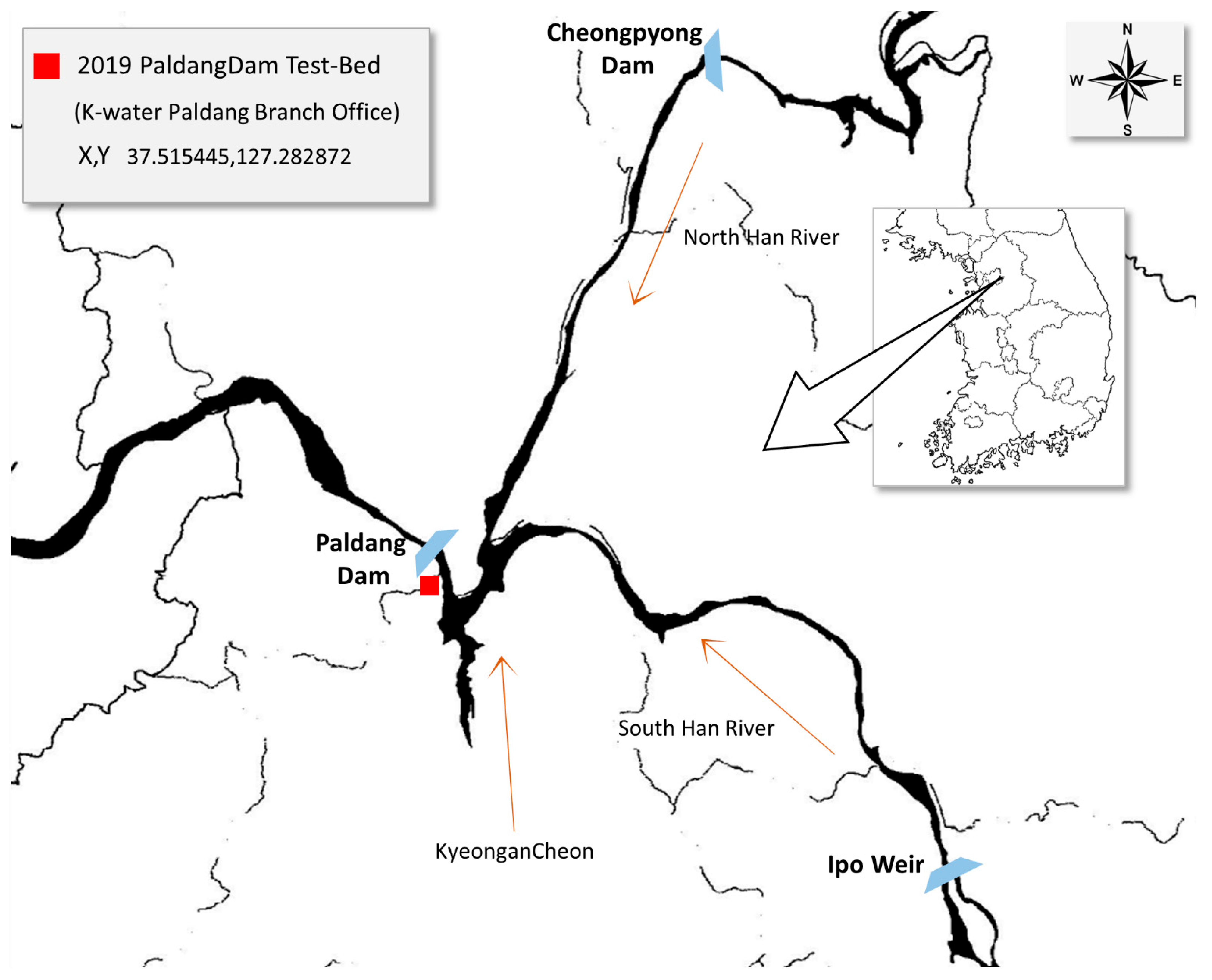
2.1. Hyperspectral Datasets
2.2. Sampling Chlorophyll-a, Hyperspectral Sensor
2.3. Data Preprocessing
2.3.1. PCA
2.3.2. PLS
2.4. Machine Learning Algorithm
2.4.1. SVR
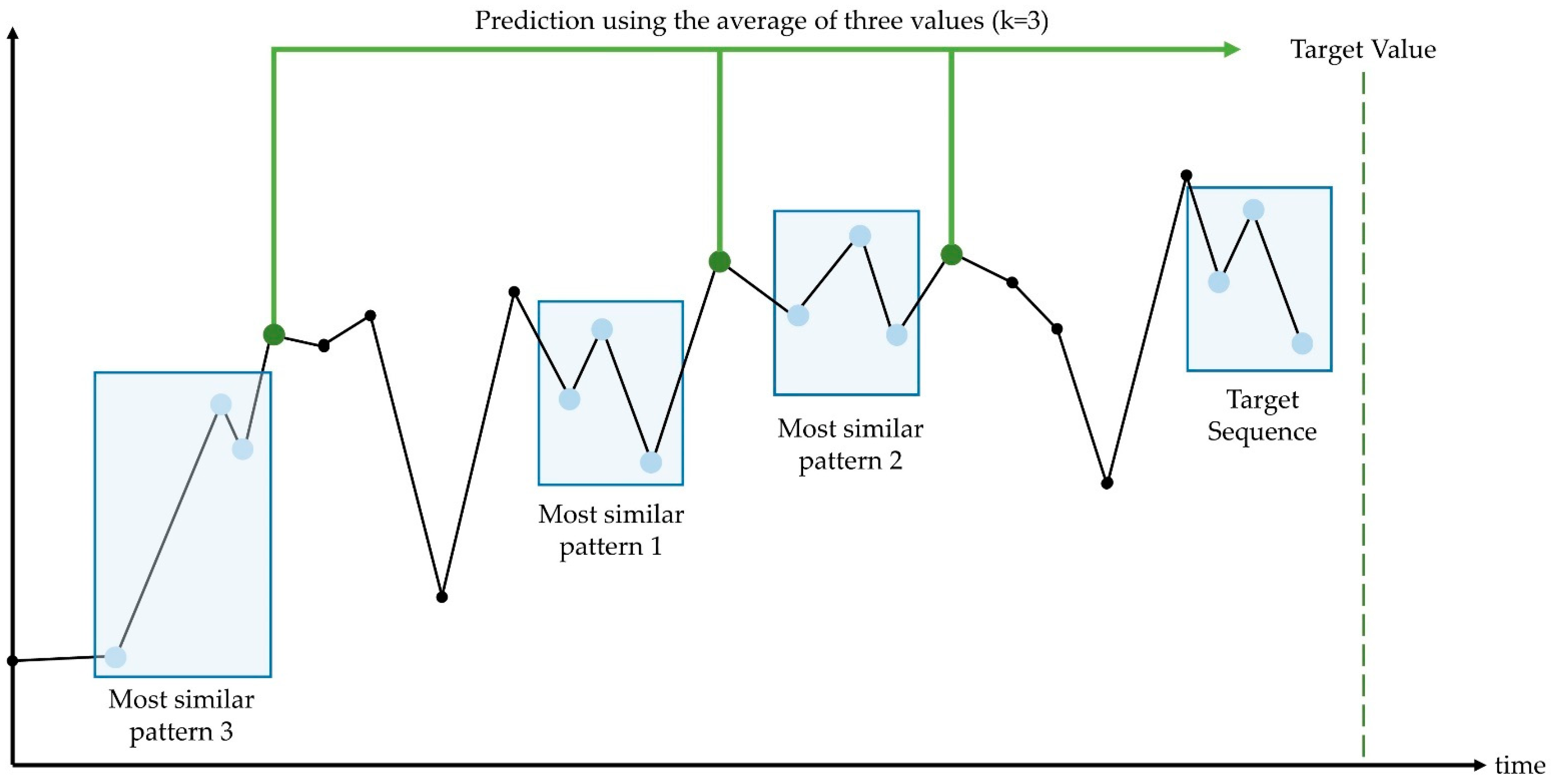
2.4.2. KNN
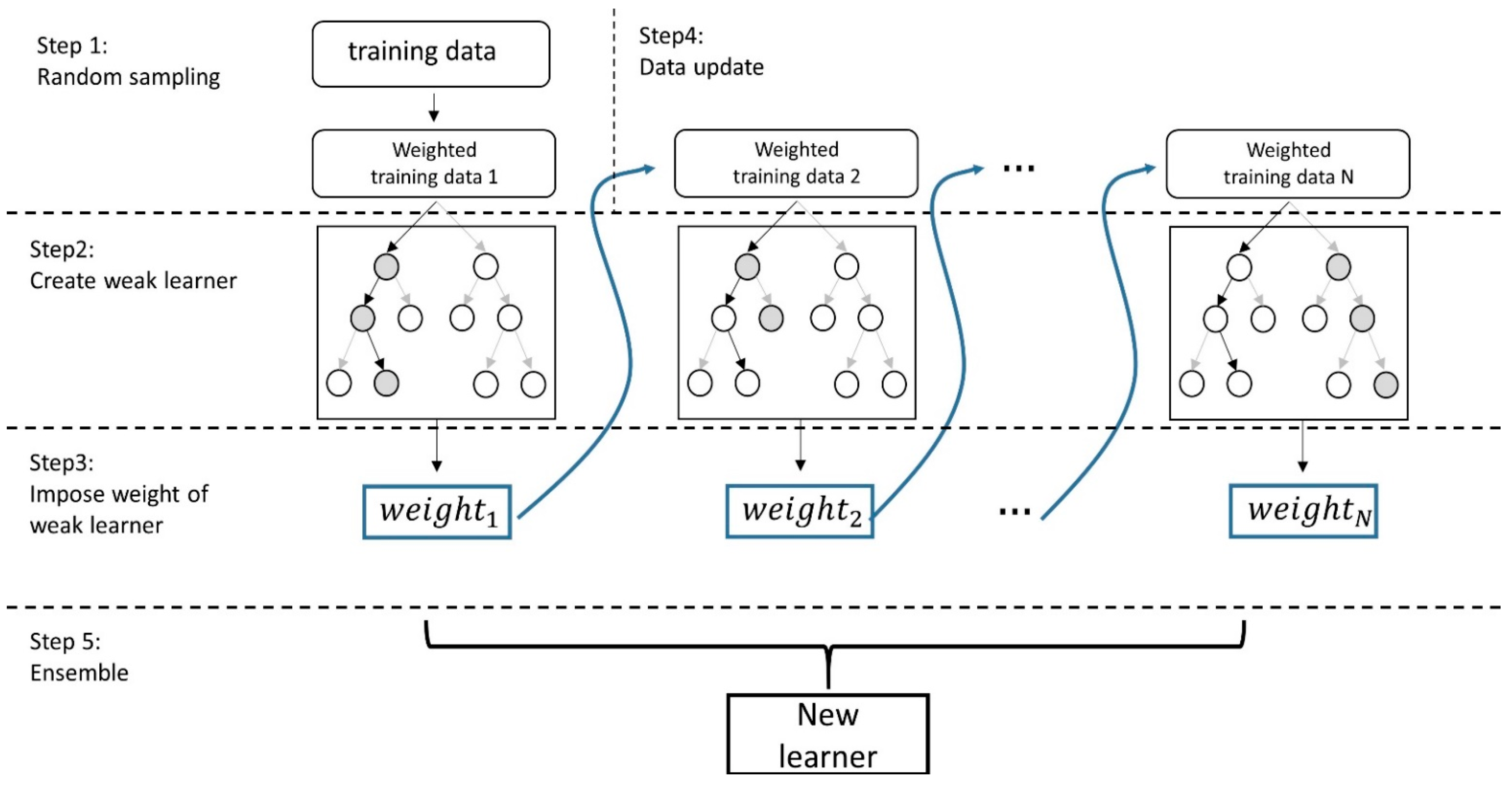
2.4.3. Bagging
2.4.4. Boosting
3. Results
3.1. Perfromance Measures
- : This is an applied evaluation metric for fit regression models that is used mainly in hydrological studies [32]. However, there is a disadvantage that increases unconditionally when the number of variables increases.
- Root mean square error (RMSE): This metric is obtained by applying the root to the mean of the total squared error (the sum of the individual squared errors). Therefore, it increases when the variance associated with the frequency distribution of error magnitudes increase [37].
- RSR (RMSE-observations standard deviation ratio): This metric standardizes RMSE using the standard deviation of the observations. Therefore, a lower RSR means better model performance and a lower RMSE [35].
- Percent bias (PBIAS): This measures the average tendency of the simulated data to be larger or smaller than their observed counterparts. That is, positive values indicate a model underestimation bias, and negative values indicate a model overestimation bias. It is useful for continuous long-term simulations and can help identify the average model simulation bias [36].
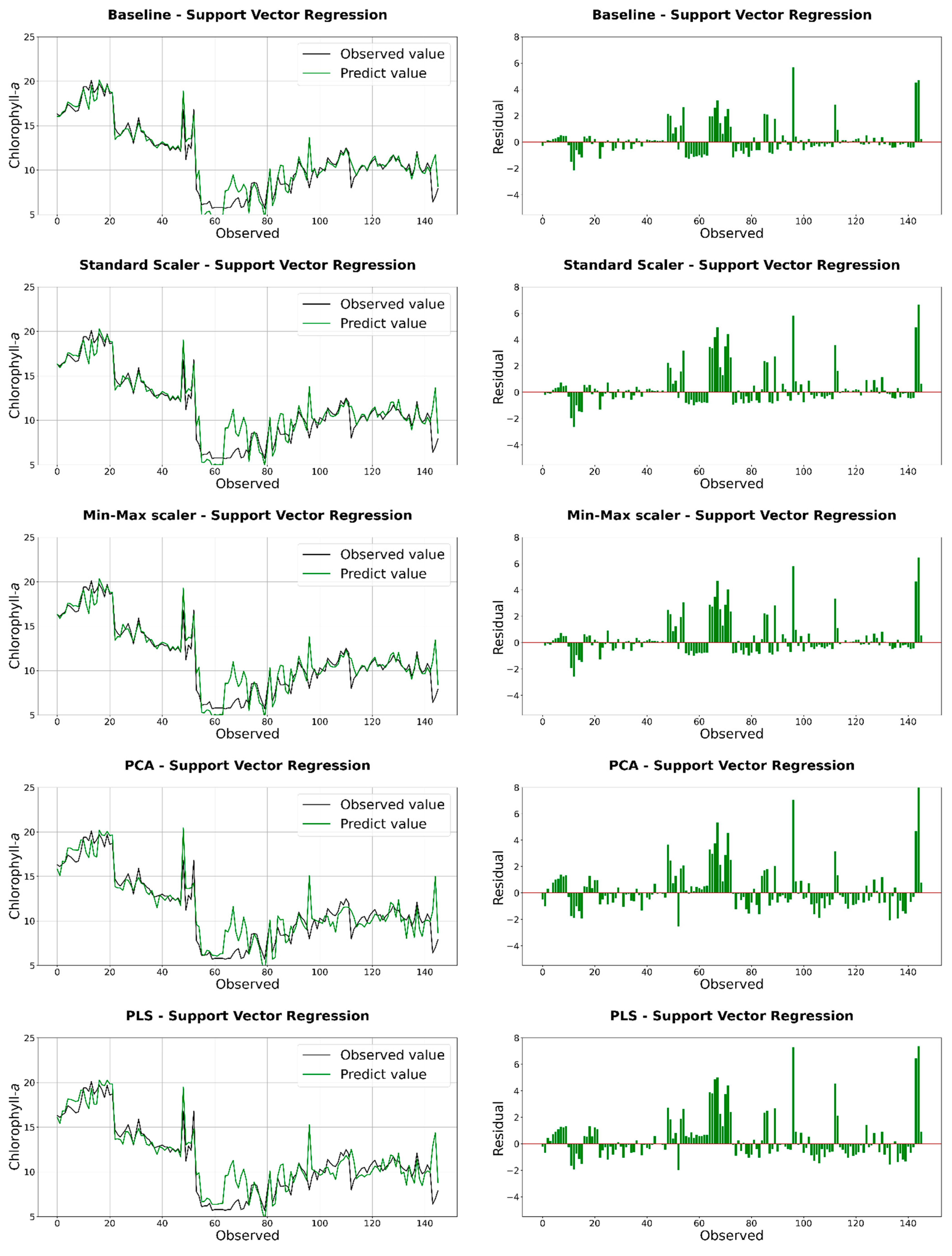
3.2. Estimation
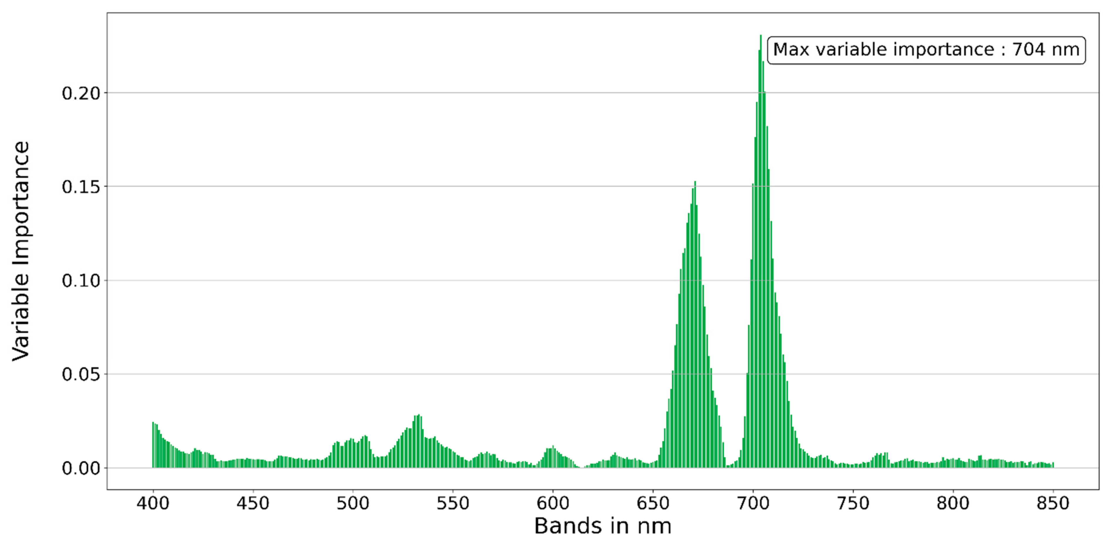
3.3. Variable Importance
4. Discussion
5. Conclusions
Author Contributions
Funding
Data Availability Statement
Conflicts of Interest
References
- Steidinger, K.A. Historical perspective on Karenia brevis red tide research in the Gulf of Mexico. Harmful Algae 2009, 8, 549–561. [Google Scholar] [CrossRef]
- Gobler, C.J. Climate change and harmful algal blooms: Insights and perspective. Harmful Algae 2020, 91, 101731. [Google Scholar] [CrossRef] [PubMed]
- Van Apeldoorn, M.E.; van Egmond, H.P.; Speijers, G.J.; Bakker, G.J. Toxins of cyanobacteria. Mol. Nutr. Food Res. 2007, 51, 7–60. [Google Scholar] [CrossRef] [PubMed]
- Paerl, H.W.; Otten, T.G. Harmful cyanobacterial blooms: Causes, consequences, and controls. Microb. Ecol. 2013, 65, 995–1010. [Google Scholar] [CrossRef]
- Min, S.K.; Son, S.W.; Seo, K.H.; Kug, J.S.; An, S.I.; Choi, Y.S.; Lee, M.I. Changes in weather and climate extremes over Korea and possible causes: A review. Asia-Pac. J. Atmos. Sci. 2015, 51, 103–121. [Google Scholar] [CrossRef]
- Hallegraeff, G.M.; Anderson, D.M.; Belin, C.; Bottein, M.-Y.D.; Bresnan, E.; Chinain, M.; Enevoldsen, H.; Iwataki, M.; Karlson, B.; McKenzie, C.H.; et al. Perceived global increase in algal blooms is attributable to intensified monitoring and emerging bloom impacts. Commun. Earth Environ. 2021, 2, 117. [Google Scholar] [CrossRef]
- Karlson, B.; Andersen, P.; Arneborg, L.; Cembella, A.; Eikrem, W.; John, U.; West, J.J.; Klemm, K.; Kobos, J.; Lehtinen, S.; et al. Harmful algal blooms and their effects in coastal seas of Northern Europe. Harmful Algae 2021, 102, 101989. [Google Scholar] [CrossRef]
- Maniyar, C.B.; Kumar, A.; Mishra, D.R. Continuous and Synoptic Assessment of Indian Inland Waters for Harmful Algae Blooms. Harmful Algae 2022, 111, 102160. [Google Scholar] [CrossRef]
- Filstrup, C.T.; Downing, J.A. Relationship of chlorophyll to phosphorus and nitrogen in nutrient-rich lakes. Inland Waters 2017, 7, 385–400. [Google Scholar] [CrossRef]
- Sellner, K.G.; Doucette, G.J.; Kirkpatrick, G.J. Harmful algal blooms: Causes, impacts and detection. J. Ind. Microbiol. Biotechnol. 2003, 30, 383–406. [Google Scholar] [CrossRef]
- Xing, Q.; Chen, C.; Shi, H.; Shi, P.; Zhang, Y. Estimation of chlorophyll-a concentrations in the Pearl River Estuary using in situ hyperspectral data: A case study. Mar. Technol. Soc. J. 2008, 42, 22–27. [Google Scholar] [CrossRef]
- Shafique, N.A.; Fulk, F.; Autrey, B.C.; Flotemersch, J. Hyperspectral remote sensing of water quality parameters for large rivers in the Ohio River basin. In Proceedings of the First Interagency Conference on Research in the Watershed, Benson, AZ, USA, 27–30 October 2003; pp. 216–221. [Google Scholar]
- Shin, Y.; Kim, T.; Hong, S.; Lee, S.; Lee, E.; Hong, S.; Lee, C.; Kim, T.; Park, M.S.; Park, J.; et al. Prediction of chlorophyll-a concentrations in the Nakdong River using machine learning methods. Water 2020, 12, 1822. [Google Scholar] [CrossRef]
- Murugan, P.; Sivakumarb, R.; Pandiyanc, R. Chlorophyll-A estimation in case-II water bodies using satellite hyperspectral data. In Proceedings of the ISPRS TC VIII International Symposium on Operational Remote Sensing Applications: Opportunities, Progress and Challenges, Hyderabad, India, 9–12 December 2014; p. 536. [Google Scholar]
- Glukhovets, D.I.; Goldin, Y.A. Express method for chlorophyll concentration assessment. J. Photochem. Photobiol. 2021, 8, 100083. [Google Scholar] [CrossRef]
- Chi, M.; Plaza, A.; Benediktsson, J.A.; Sun, Z.; Shen, J.; Zhu, Y. Big Data for Remote Sensing: Challenges and Opportunities. Proc. IEEE 2016, 104, 2207–2219. [Google Scholar] [CrossRef]
- Keller, S.; Maier, P.M.; Riese, F.M.; Norra, S.; Holbach, A.; Börsig, N.; Wilhelms, A.; Moldaenke, C.; Zaake, A.; Hinz, S. Hyperspectral data and machine learning for estimating CDOM, chlorophyll a, diatoms, green algae and turbidity. Int. J. Environ. Res. Public Health 2018, 15, 1881. [Google Scholar] [CrossRef] [Green Version]
- Geurts, P.; Ernst, D.; Wehenkel, L. Extremely randomized trees. Mach. Learn. 2006, 63, 3–42. [Google Scholar] [CrossRef] [Green Version]
- Levy, J.; Cary, S.; Joy, K.; Lee, C. Detection and community-level identification of microbial mats in the McMurdo Dry Valleys using drone-based hyperspectral reflectance imaging. Antarct. Sci. 2020, 32, 367–381. [Google Scholar] [CrossRef]
- Wold, S.; Esbensen, K.; Geladi, P. Principal component analysis. Chemom. Intell. Lab. Syst. 1987, 2, 37–52. [Google Scholar] [CrossRef]
- Kim, D.W.; Min, J.H.; Yoo, M.; Kang, M.; Kim, K. Long-term effects of hydrometeorological and water quality conditions on algal dynamics in the Paldang dam watershed, Korea. Water Sci. Technol. Water Supply 2014, 14, 601–608. [Google Scholar] [CrossRef]
- Li, Z.; Shin, H.H.; Lee, T.; Han, M.S. Resting stages of freshwater algae from surface sediments in Paldang Dam Lake, Korea. Nova Hedwig. 2015, 101, 475–500. [Google Scholar] [CrossRef]
- Peters, S.; Laanen, M.; Groetsch, P.; Ghezehegn, S.; Poser, K.; Hommersom, A.; de Reus, E.; Spaias, L. WISPstation: A new autonomous above water radiometer system. In Proceedings of the Ocean Optics XXIV Conference, Dubrovnik, Croatia, 7–12 October 2018; pp. 7–12. [Google Scholar]
- Lee, D.H.; Woo, S.E.; Jung, M.W.; Heo, T.Y. Evaluation of Odor Prediction Model Performance and Variable Importance according to Various Missing Imputation Methods. Appl. Sci. 2022, 12, 2826. [Google Scholar] [CrossRef]
- Smola, A.J.; Schölkopf, B. A tutorial on support vector regression. Stat. Comput. 2004, 14, 199–222. [Google Scholar] [CrossRef] [Green Version]
- Altman, N.S. An introduction to kernel and nearest-neighbor nonparametric regression. Am. Stat. 1992, 46, 175–185. [Google Scholar]
- Breiman, L. Random forests. Mach. Learn. 2001, 45, 5–32. [Google Scholar] [CrossRef] [Green Version]
- Freund, Y.; Schapire, R.E. A decision-theoretic generalization of on-line learning and an application to boosting. J. Comput. Syst. Sci. 1997, 55, 119–139. [Google Scholar] [CrossRef] [Green Version]
- Friedman, J.H. Stochastic gradient boosting. Comput. Stat. Data Anal. 2002, 38, 367–378. [Google Scholar] [CrossRef]
- Chen, T.; Guestrin, C. Xgboost: A scalable tree boosting system. In Proceedings of the 22nd ACM SIGKDD International Conference on Knowledge Discovery and Data Mining, San Francisco, CA, USA, 13–17 August 2016; pp. 785–794. [Google Scholar]
- Moriasi, D.N.; Gitau, M.W.; Pai, N.; Daggupati, P. Hydrologic and water quality models: Performance measures and evaluation criteria. Trans. ASABE 2015, 58, 1763–1785. [Google Scholar]
- Zeybek, M. Nash-sutcliffe efficiency approach for quality improvement. J. Appl. Math. Comput. 2018, 2, 496–503. [Google Scholar] [CrossRef]
- Legates, D.R.; McCabe, G.J., Jr. Evaluating the use of “goodness-of-fit” measures in hydrologic and hydroclimatic model validation. Water Resour. Res. 1999, 35, 233–241. [Google Scholar] [CrossRef]
- Moriasi, D.N.; Arnold, J.G.; van Liew, M.W.; Bingner, R.L.; Harmel, R.D.; Veith, T.L. Model evaluation guidelines for systematic quantification of accuracy in watershed simulations. Trans. ASABE 2007, 50, 885–900. [Google Scholar] [CrossRef]
- Gupta, H.V.; Sorooshian, S.; Yapo, P.O. Status of automatic calibration for hydrologic models: Comparison with multilevel expert calibration. J. Hydrol. Eng. 1999, 4, 135–143. [Google Scholar] [CrossRef]
- Willmott, C.J.; Matsuura, K. Advantages of the mean absolute error (MAE) over the root mean square error (RMSE) in assessing average model performance. Clim. Res. 2005, 30, 79–82. [Google Scholar] [CrossRef]
- Pyo, J.; Hong, S.M.; Jang, J.; Park, S.; Park, J.; Noh, J.H.; Cho, K.H. Drone-borne sensing of major and accessory pigments in algae using deep learning modeling. GIScience Remote Sens. 2022, 59, 310–332. [Google Scholar] [CrossRef]
- Wong, K.T.; Lee, J.H.; Hodgkiss, I.J. A simple model for forecast of coastal algal blooms. Estuar. Coast. Shelf Sci. 2007, 74, 175–196. [Google Scholar] [CrossRef]
- Huh, J.H.; Choi, Y.H.; Lee, H.J.; Choi, W.J.; Ramakrishna, C.; Lee, H.W.; Lee, S.-H.; Ahn, J.W. The use of oyster shell powders for water quality improvement of lakes by algal blooms removal. J. Korean Ceram. Soc. 2016, 53, 1–6. [Google Scholar] [CrossRef] [Green Version]
- Zhu, W.; Sun, Z.; Yang, T.; Li, J.; Peng, J.; Zhu, K.; Li, S.; Gong, H.; Lyu, Y.; Li, B.; et al. Estimating leaf chlorophyll content of crops via optimal unmanned aerial vehicle hyperspectral data at multi-scales. Comput. Electron. Agric. 2020, 178, 105786. [Google Scholar] [CrossRef]
- Gai, Y.; Yu, D.; Zhou, Y.; Yang, L.; Chen, C.; Chen, J. An improved model for chlorophyll-a concentration retrieval in coastal waters based on UAV-Borne hyperspectral imagery: A case study in Qingdao, China. Water 2020, 12, 2769. [Google Scholar] [CrossRef]


| Metric | Equation | Range (Optimal Value) |
|---|---|---|
| 0.0~1.0 (1.0) | ||
| NSE | −∞~1.0 (1.0) | |
| d | 0.0~1.0 (1.0) | |
| RMSE | 0.0~∞ (0.0) | |
| RSR | 0.0~∞ (0.0) | |
| PBIAS | −∞~∞ (0.0) |
| Method | MSE | MAPE | NSE | d | PSR | ||
|---|---|---|---|---|---|---|---|
| Baseline | OLS | 0.380 | 126.665 | 77.598 | −7.592 | 0.402 | 2.121 |
| RF | 0.919 | 20.070 | 44.153 | −0.361 | 0.557 | 0.922 | |
| ET | 0.986 | 18.878 | 42.474 | −0.281 | 0.569 | 0.912 | |
| GB | 0.941 | 12.765 | 33.110 | 0.134 | 0.701 | 0.809 | |
| AdaBoost | 0.908 | 22.93 | 47.754 | −0.555 | 0.502 | 0.963 | |
| KNN | 0.925 | 17.284 | 39.489 | −0.172 | 0.617 | 0.898 | |
| SVR | 0.991 | 1.299 | 8.365 | 0.912 | 0.977 | 0.297 | |
| XGBoost | 0.948 | 10.908 | 30.194 | 0.26 | 0.742 | 0.765 | |
| Standard Scaler | OLS | 0.122 | 337.646 | 178.614 | −21.904 | 0.305 | 1.04 |
| RF | 0.919 | 19.967 | 43.996 | −0.354 | 0.558 | 0.921 | |
| ET | 0.986 | 18.918 | 42.529 | −0.283 | 0.568 | 0.913 | |
| GB | 0.947 | 11.282 | 31.21 | 0.235 | 0.732 | 0.772 | |
| AdaBoost | 0.908 | 23.348 | 48.034 | −0.584 | 0.507 | 0.963 | |
| KNN | 0.929 | 16.617 | 39.044 | −0.127 | 0.632 | 0.882 | |
| SVR | 0.986 | 2.132 | 10.473 | 0.855 | 0.961 | 0.379 | |
| XGBoost | 0.948 | 10.908 | 30.194 | 0.260 | 0.742 | 0.765 | |
| Min-Max scaler | OLS | 0.737 | 45.016 | 48.533 | −2.054 | 0.685 | 1.604 |
| RF | 0.919 | 19.967 | 43.996 | −0.354 | 0.558 | 0.921 | |
| ET | 0.986 | 18.878 | 42.474 | −0.281 | 0.569 | 0.912 | |
| GB | 0.947 | 11.282 | 31.21 | 0.235 | 0.732 | 0.772 | |
| AdaBoost | 0.908 | 23.348 | 48.034 | −0.584 | 0.507 | 0.963 | |
| KNN | 0.930 | 16.797 | 39.028 | −0.139 | 0.632 | 0.879 | |
| SVR | 0.987 | 1.950 | 10.113 | 0.868 | 0.965 | 0.363 | |
| XGBoost | 0.948 | 10.908 | 30.194 | 0.260 | 0.742 | 0.765 | |
| PCA | OLS | 0.170 | 330.055 | 184.408 | −21.389 | 0.314 | 1.003 |
| RF | 0.964 | 6.675 | 23.326 | 0.547 | 0.853 | 0.636 | |
| ET | 0.986 | 5.820 | 22.345 | 0.605 | 0.861 | 0.589 | |
| GB | 0.980 | 3.428 | 16.316 | 0.767 | 0.935 | 0.472 | |
| AdaBoost | 0.962 | 8.479 | 27.148 | 0.425 | 0.82 | 0.68 | |
| KNN | 0.928 | 16.752 | 39.179 | −0.136 | 0.63 | 0.884 | |
| SVR | 0.982 | 2.602 | 11.776 | 0.824 | 0.953 | 0.419 | |
| XGBoost | 0.981 | 3.229 | 15.499 | 0.781 | 0.935 | 0.459 | |
| PLS | OLS | 0.171 | 330.243 | 184.598 | −21.402 | 0.314 | 1.002 |
| RF | 0.983 | 4.291 | 17.468 | 0.709 | 0.928 | 0.51 | |
| ET | 0.986 | 4.475 | 20.171 | 0.696 | 0.905 | 0.514 | |
| GB | 0.988 | 1.875 | 10.351 | 0.873 | 0.969 | 0.356 | |
| AdaBoost | 0.977 | 7.481 | 25.6 | 0.493 | 0.868 | 0.625 | |
| KNN | 0.932 | 14.624 | 36.223 | 0.008 | 0.663 | 0.861 | |
| SVR | 0.981 | 2.828 | 12.363 | 0.808 | 0.948 | 0.436 | |
| XGBoost | 0.990 | 1.595 | 10.416 | 0.892 | 0.972 | 0.327 | |
| ML Model (with Preprocessing) | Hyperparameters | Type | Search Space | Optimal Parameters |
|---|---|---|---|---|
| OLS | - | - | - | - |
| Random Forest (PLS) | min_samples_leaf | Discrete | 3, 5, 7, 10 | 3 |
| max_depth | Discrete | 3, 4, 5, 6 | 6 | |
| Extreme Tree (PLS) | min_samples_leaf | Discrete | 3, 5, 7, 10 | 5 |
| max_depth | Discrete | 3, 4, 5, 6 | 6 | |
| Gradient Boost (PLS) | min_samples_leaf | Discrete | 3, 5, 7, 10 | 10 |
| n_estimators | Discrete | 100, 200, 300 | 300 | |
| AdaBoost (PLS) | n_estimators | Discrete | 100, 200, 300 | 300 |
| learning_rate | Discrete | 0.1, 0.05, 0.02, 0.01 | 0.1 | |
| KNN (PLS) | n_neighbrs | Discrete | 3,5,7,9,11, | 5 |
| weights | Categorical | “uniform”, “distance” | distance | |
| algorithm | Categorical | “ball_tree”, “kd_tree”, “brute” | ball_tree | |
| SVR (Baseline) | Kernel | Categorical | “rbf”, “sigmoid” | rbf |
| C | Discrete | 10,30,100,300,1000 | 1000 | |
| XGBoost (PLS) | max_depth | Discrete | 5, 6, 7 | 5 |
| learning_rate | Discrete | 0.03, 0.05, 0.07 | 0.07 |
Publisher’s Note: MDPI stays neutral with regard to jurisdictional claims in published maps and institutional affiliations. |
© 2022 by the authors. Licensee MDPI, Basel, Switzerland. This article is an open access article distributed under the terms and conditions of the Creative Commons Attribution (CC BY) license (https://creativecommons.org/licenses/by/4.0/).
Share and Cite
Im, G.; Lee, D.; Lee, S.; Lee, J.; Lee, S.; Park, J.; Heo, T.-Y. Estimating Chlorophyll-a Concentration from Hyperspectral Data Using Various Machine Learning Techniques: A Case Study at Paldang Dam, South Korea. Water 2022, 14, 4080. https://doi.org/10.3390/w14244080
Im G, Lee D, Lee S, Lee J, Lee S, Park J, Heo T-Y. Estimating Chlorophyll-a Concentration from Hyperspectral Data Using Various Machine Learning Techniques: A Case Study at Paldang Dam, South Korea. Water. 2022; 14(24):4080. https://doi.org/10.3390/w14244080
Chicago/Turabian StyleIm, GwangMuk, Dohyun Lee, Sanghun Lee, Jongsu Lee, Sungjong Lee, Jungsu Park, and Tae-Young Heo. 2022. "Estimating Chlorophyll-a Concentration from Hyperspectral Data Using Various Machine Learning Techniques: A Case Study at Paldang Dam, South Korea" Water 14, no. 24: 4080. https://doi.org/10.3390/w14244080
APA StyleIm, G., Lee, D., Lee, S., Lee, J., Lee, S., Park, J., & Heo, T.-Y. (2022). Estimating Chlorophyll-a Concentration from Hyperspectral Data Using Various Machine Learning Techniques: A Case Study at Paldang Dam, South Korea. Water, 14(24), 4080. https://doi.org/10.3390/w14244080