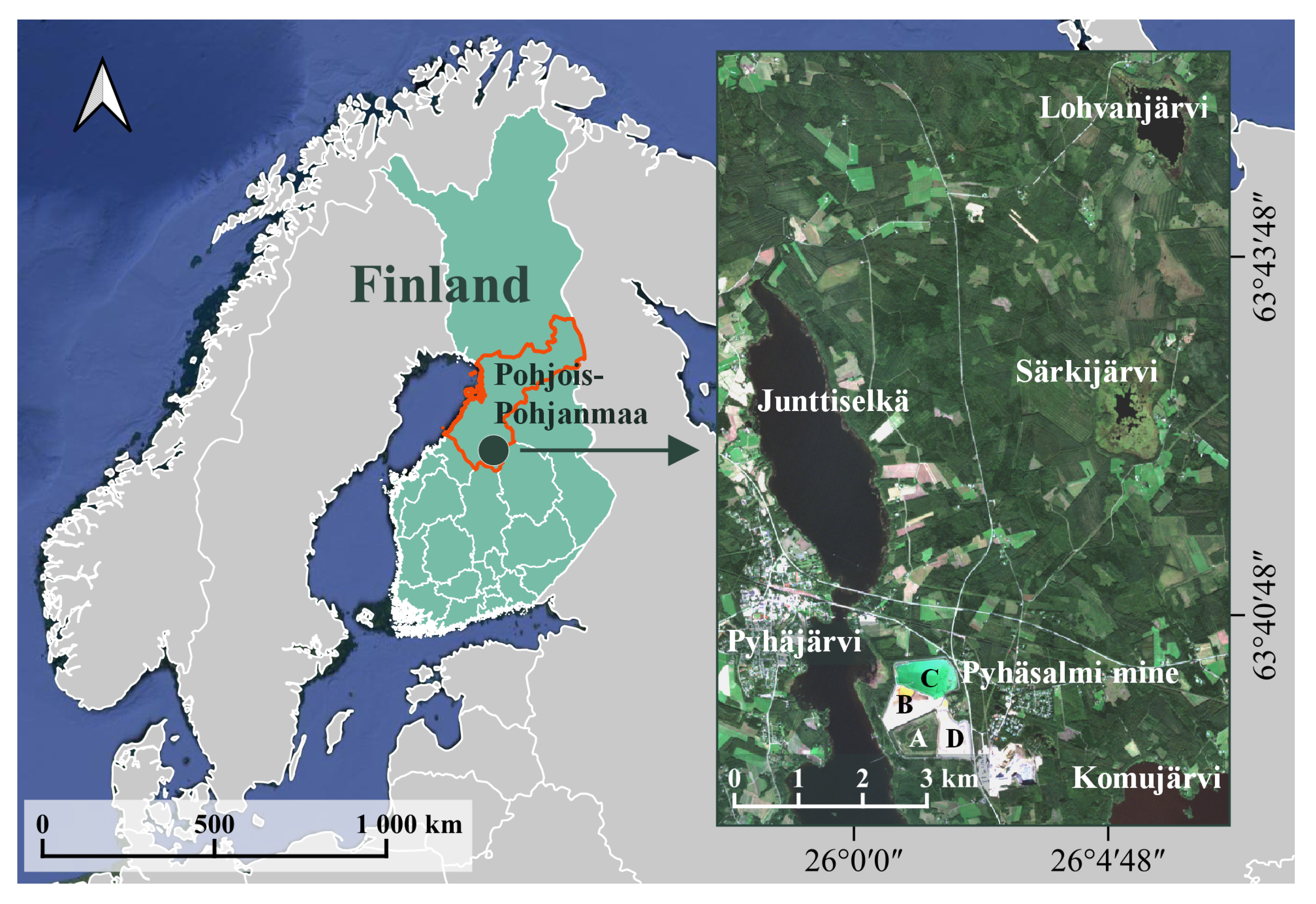
Figure 1.
Study area in Pohjois-Pohjanmaa region (Finland). Basemap: Google Earth Satellite (EPSG:4326–WGS 84).
Figure 1.
Study area in Pohjois-Pohjanmaa region (Finland). Basemap: Google Earth Satellite (EPSG:4326–WGS 84).
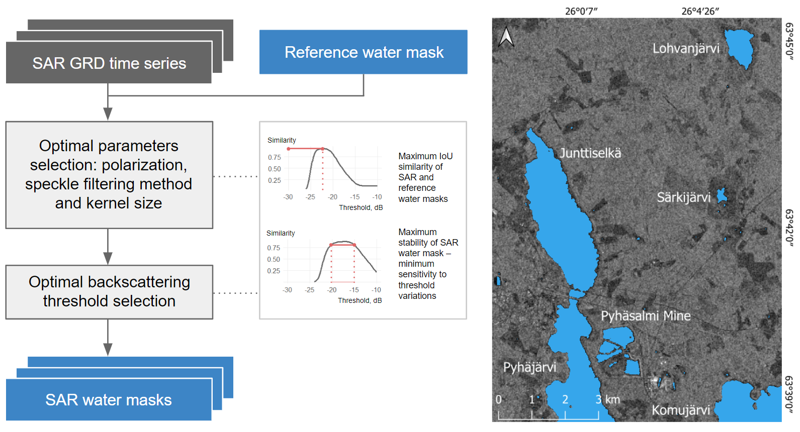
Figure 2.
Optimal threshold selection algorithm workflow.
Figure 2.
Optimal threshold selection algorithm workflow.
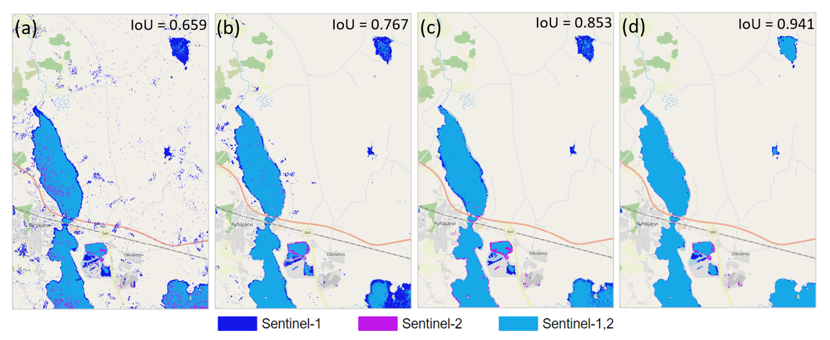
Figure 3.
Maps of optical and SAR masks of surface water bodies with different IoU values: (a) 23 May 2019, path 153, VV polarization, MNDWI, without speckle filtering (IoU = 0.659); (b) 28 May 2018, path 160, VH polarization, NDWI, Median 3 × 3 speckle filtering (IoU = 0.767); (c) 23 May 2019, path 153, VH polarization, NDWI, Lee 7 × 7 speckle filtering (IoU = 0.853); (d) 28 August 2021, path 160, VH polarization, MNDWI, Median 7 × 7 speckle filtering (IoU = 0.941). Basemap: OpenStreetMap Standard.
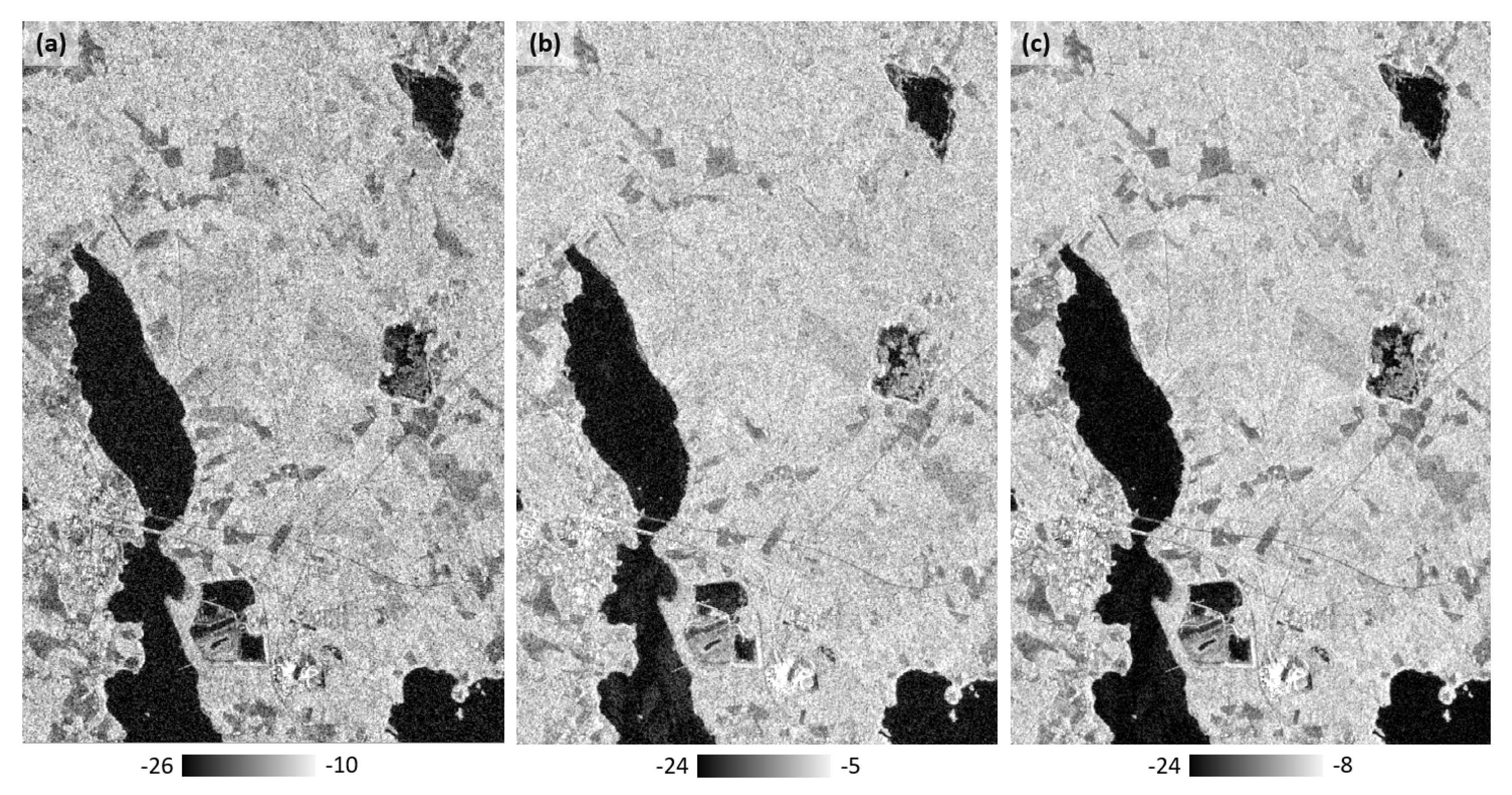
Figure 4.
Sentinel-1 backscattering coefficients of study area without speckle-filtering, 12 May 2021, path 153: (a) ; (b) ; and (c) .
Figure 4.
Sentinel-1 backscattering coefficients of study area without speckle-filtering, 12 May 2021, path 153: (a) ; (b) ; and (c) .
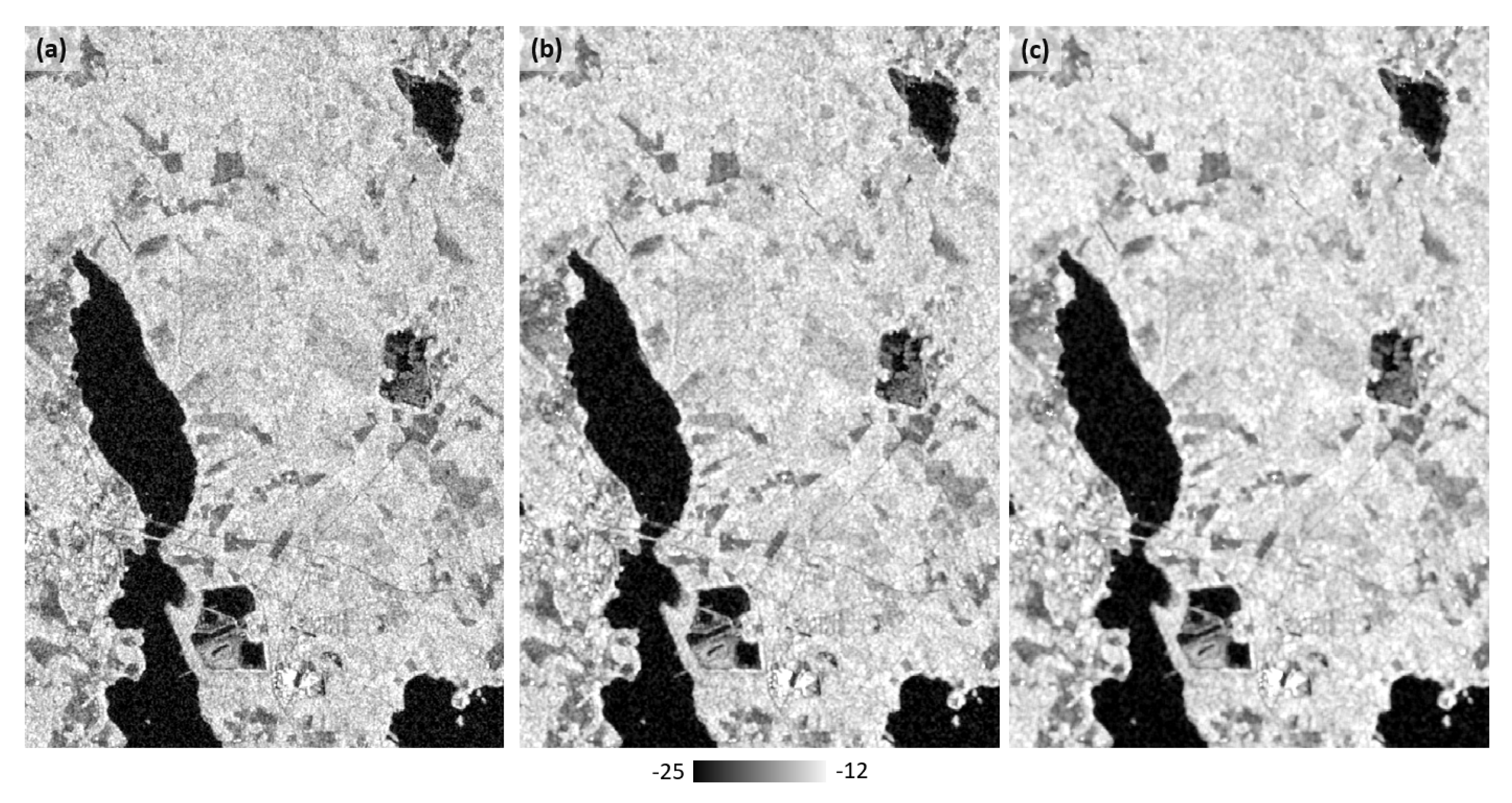
Figure 5.
Sentinel-1 backscattering coefficients of study area after Lee speckle filtering with kernel sizes: (a) 3 × 3; (b) 5 × 5; and (c) 7 × 7; 12 May 2021, path 153.
Figure 5.
Sentinel-1 backscattering coefficients of study area after Lee speckle filtering with kernel sizes: (a) 3 × 3; (b) 5 × 5; and (c) 7 × 7; 12 May 2021, path 153.
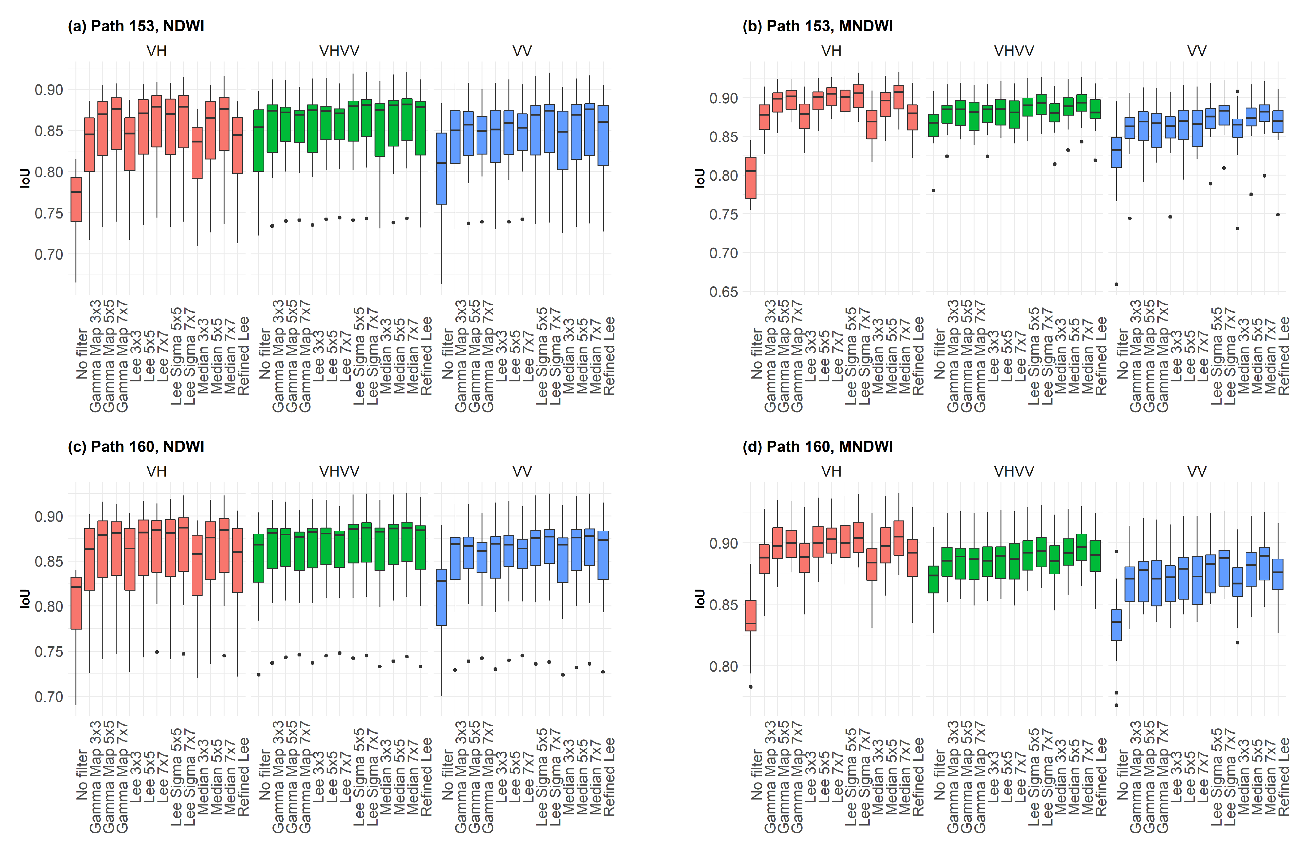
Figure 6.
IoU box-plot chart for various reference masks, polarizations, and speckle filtering parameters: (a) path 153, NDWI; (b) path 153, MNDWI; (c) path 160, NDWI; and (d) path 160, MNDWI.
Figure 6.
IoU box-plot chart for various reference masks, polarizations, and speckle filtering parameters: (a) path 153, NDWI; (b) path 153, MNDWI; (c) path 160, NDWI; and (d) path 160, MNDWI.
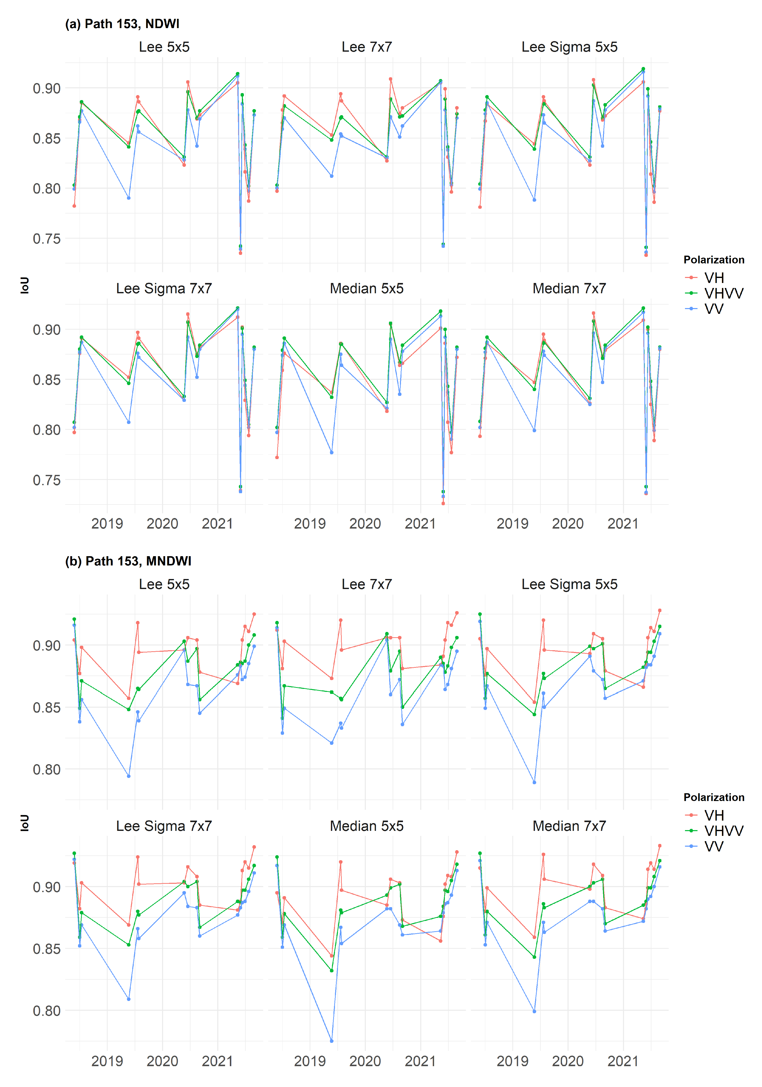
Figure 7.
IoU-similarity plots over time for various polarizations and speckle filtering parameters: (a) path 153, NDWI and (b) path 153, MNDWI.
Figure 7.
IoU-similarity plots over time for various polarizations and speckle filtering parameters: (a) path 153, NDWI and (b) path 153, MNDWI.
Figure 8.
IoU mask similarity versus backscatter threshold: (a) 22 July 2019 NDWI; (b) 22 July 2019 MNDWI.
Figure 8.
IoU mask similarity versus backscatter threshold: (a) 22 July 2019 NDWI; (b) 22 July 2019 MNDWI.
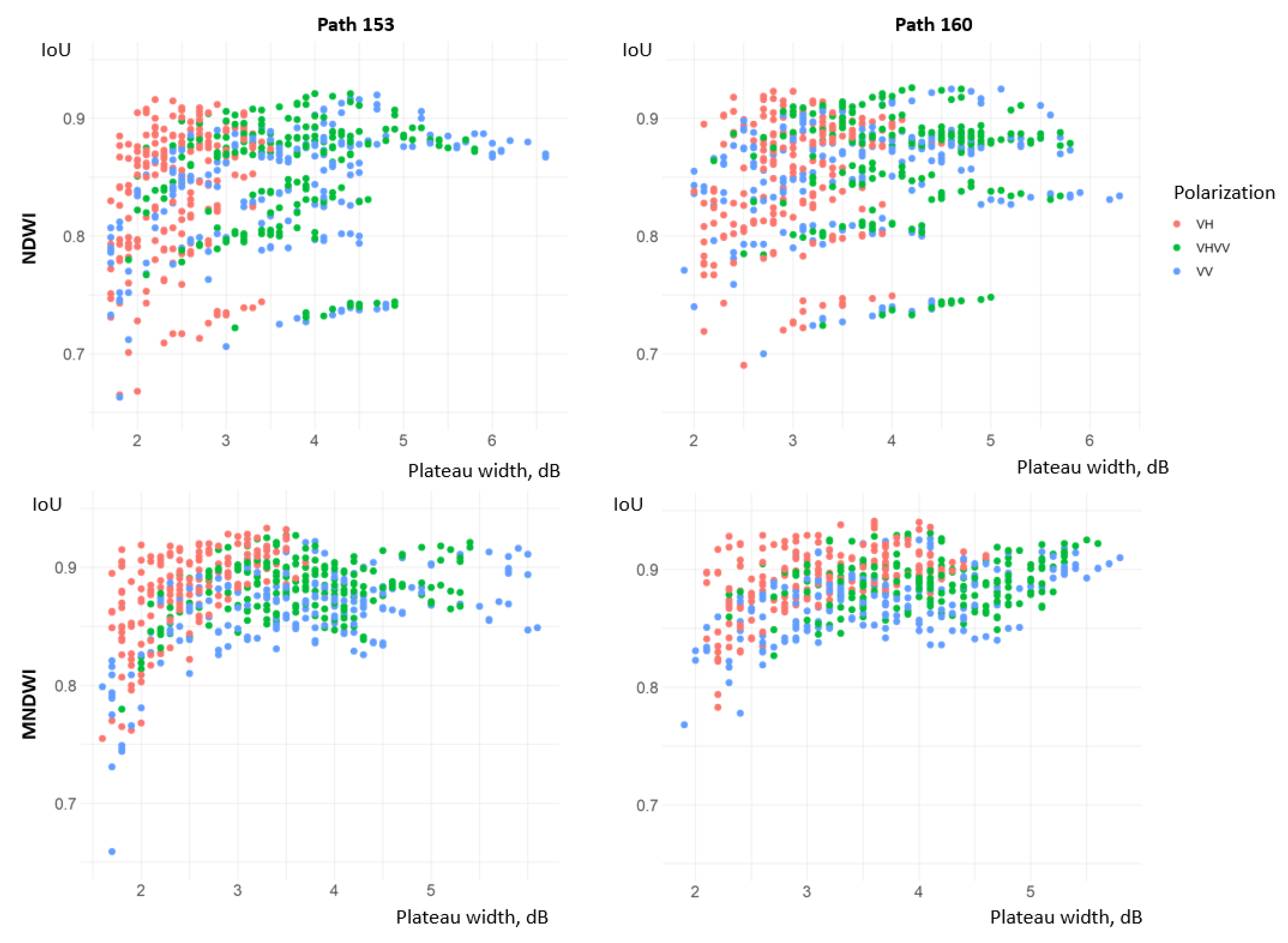
Figure 9.
Scatterplots of IoU values versus plateau width.
Figure 9.
Scatterplots of IoU values versus plateau width.
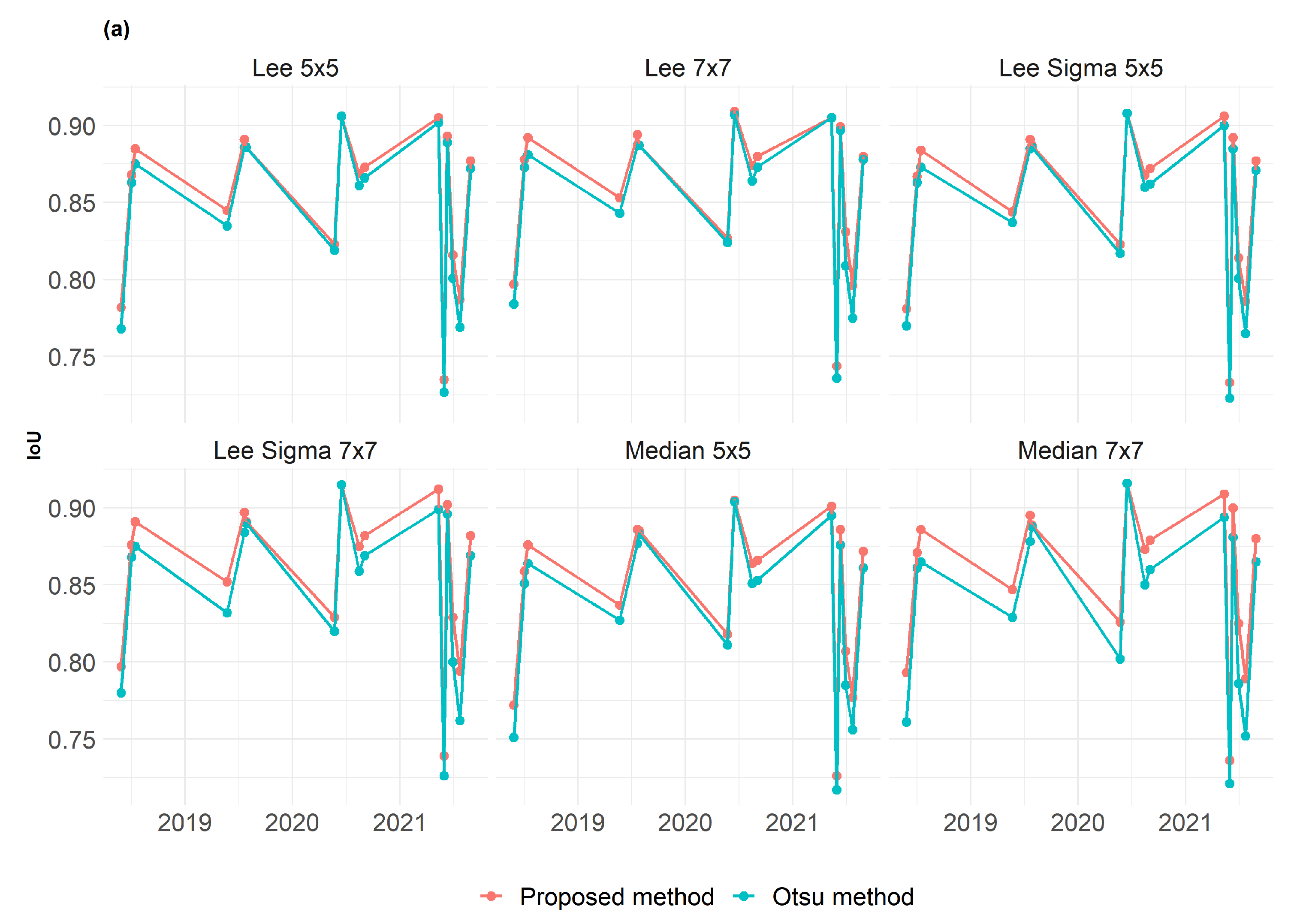
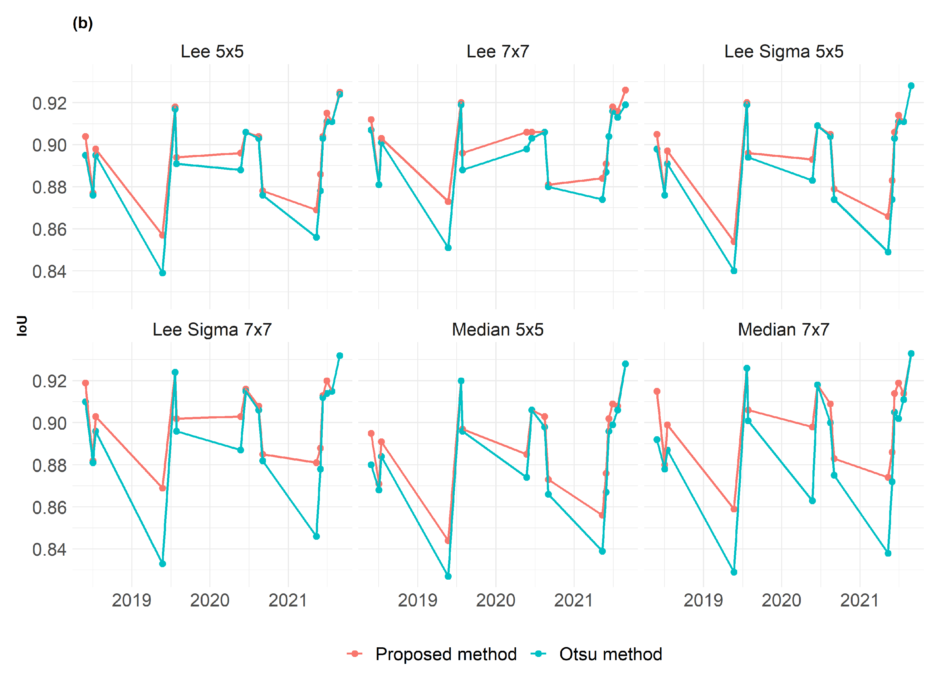
Figure 10.
IoU-similarity over time for the proposed method and the Otsu method with different speckle filtering parameters.
Figure 10.
IoU-similarity over time for the proposed method and the Otsu method with different speckle filtering parameters.
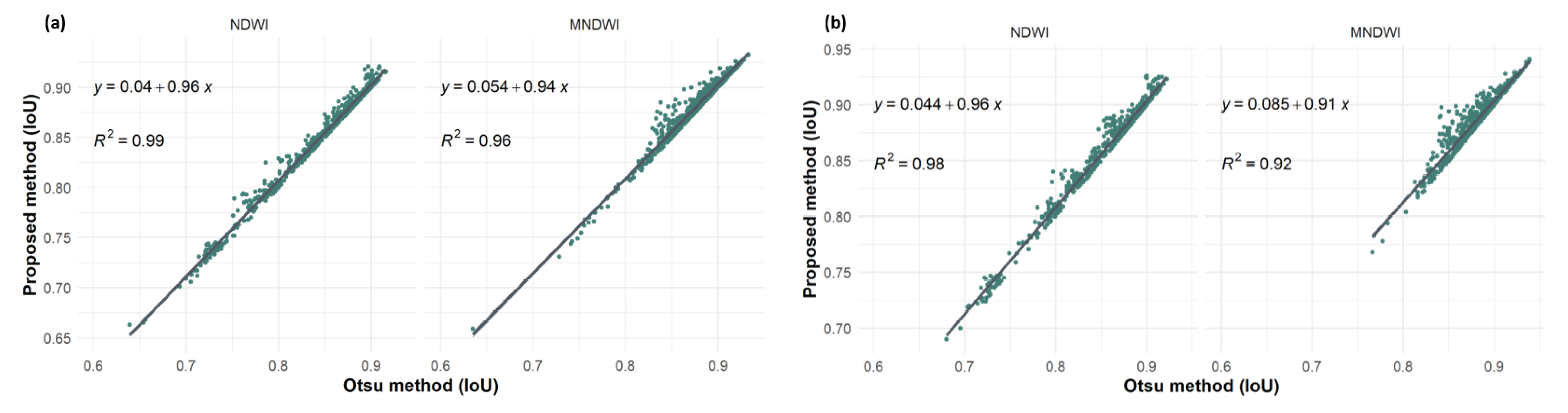
Figure 11.
Plots of IoU correlation between the proposed method and the Otsu method: (a) path 153 and (b) path 160.
Figure 11.
Plots of IoU correlation between the proposed method and the Otsu method: (a) path 153 and (b) path 160.
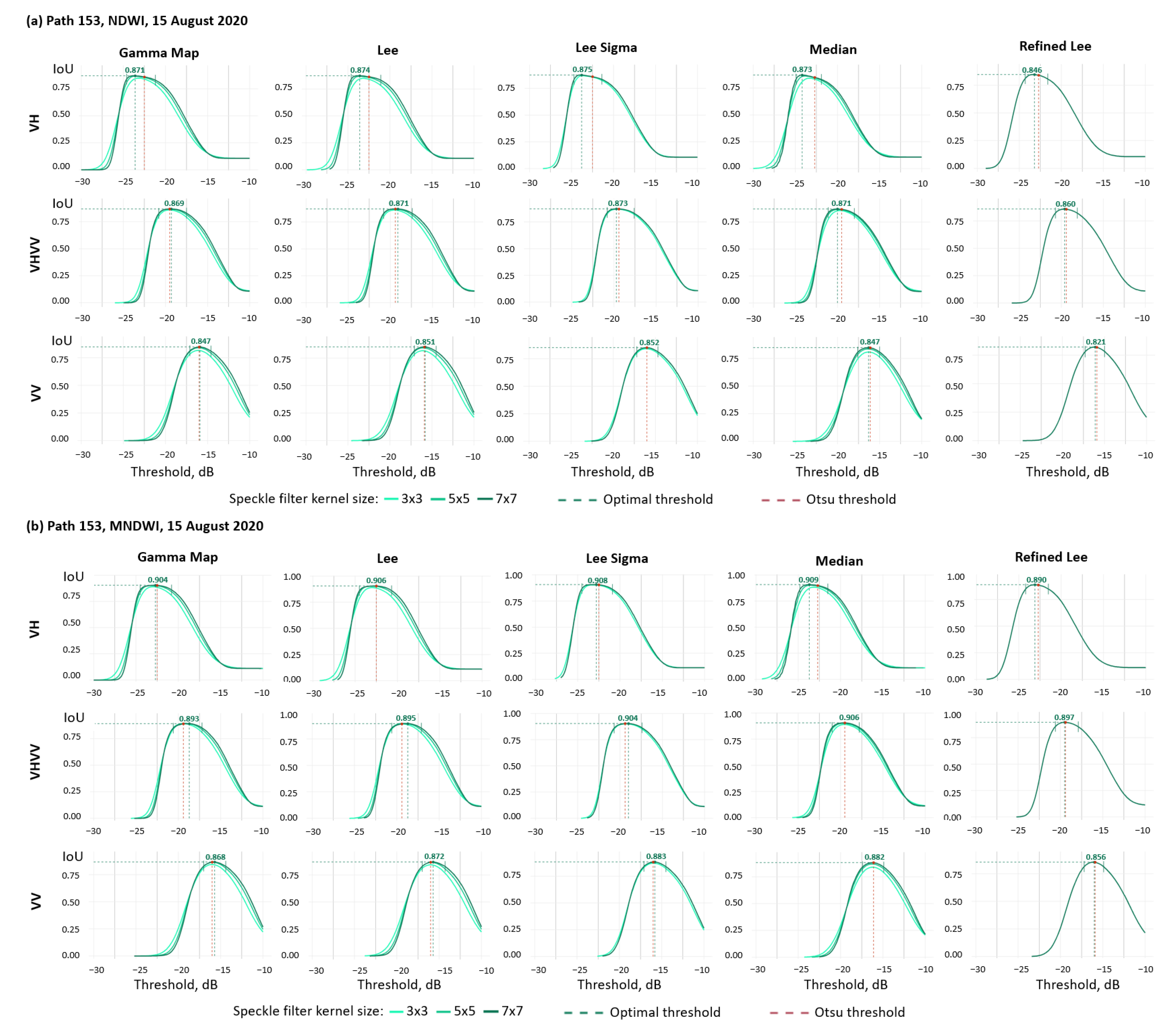
Figure 12.
Comparison of the thresholds determined using the proposed method and the Otsu method on the plots of mask similarity (IoU) versus backscatter threshold: (a) 15 August 2020 NDWI and (b) 15 August 2020 MNDWI.
Figure 12.
Comparison of the thresholds determined using the proposed method and the Otsu method on the plots of mask similarity (IoU) versus backscatter threshold: (a) 15 August 2020 NDWI and (b) 15 August 2020 MNDWI.
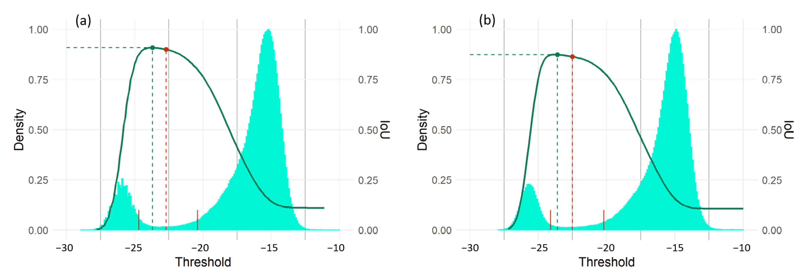
Figure 13.
Visualization of optimal thresholds determined by the proposed method (green dotted line) and by the Otsu method (red dotted line) on IoU curves and histograms on 15 August 2020: (a) MNDWI Median 7 × 7; (b) NDWI Lee 7 × 7.
Figure 13.
Visualization of optimal thresholds determined by the proposed method (green dotted line) and by the Otsu method (red dotted line) on IoU curves and histograms on 15 August 2020: (a) MNDWI Median 7 × 7; (b) NDWI Lee 7 × 7.
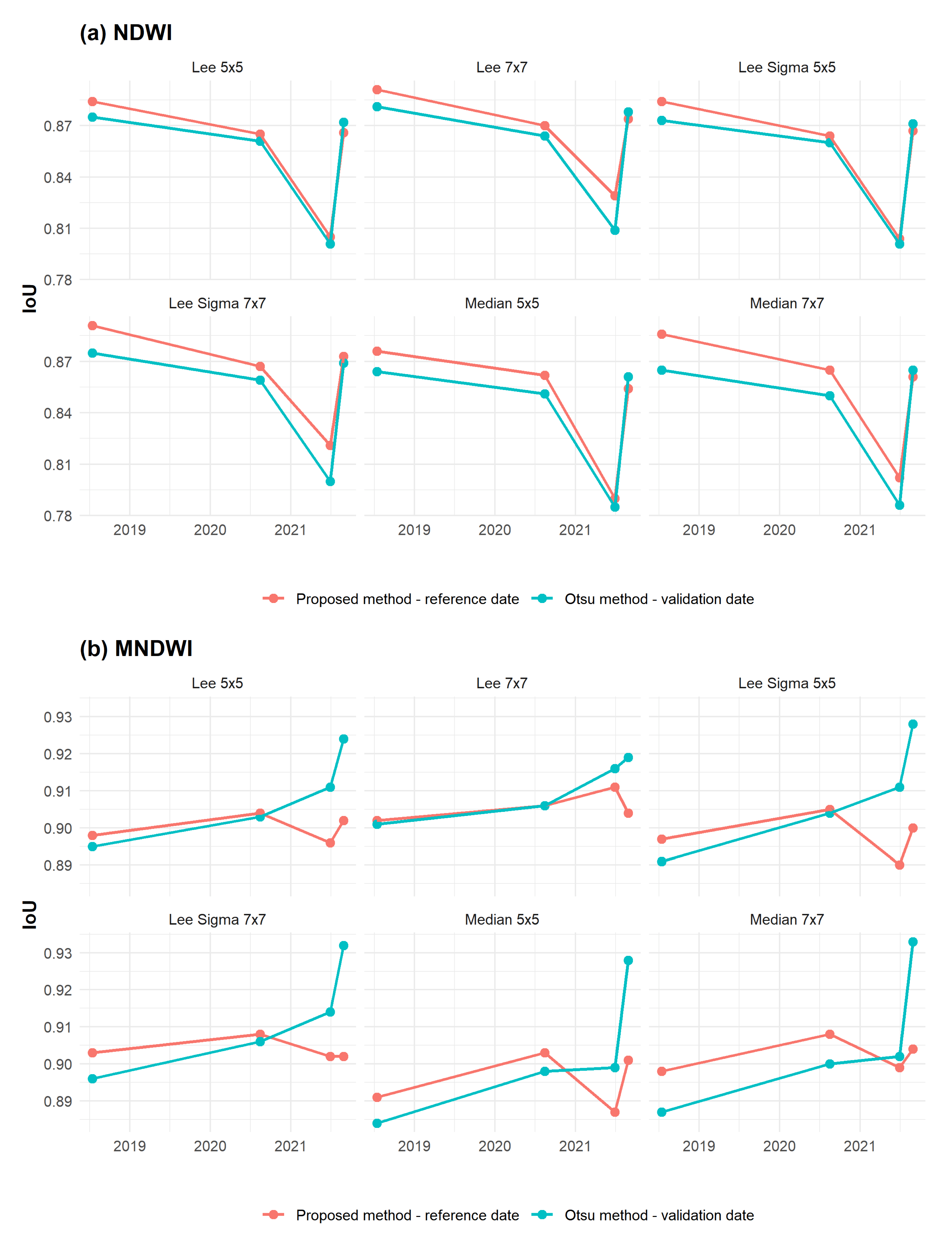
Figure 14.
Comparison of the accuracy of optimal thresholds determined on reference dates and applied on validation dates with thresholds determined on validation dates using the Otsu method: (a) NDWI and (b) MNDWI.
Figure 14.
Comparison of the accuracy of optimal thresholds determined on reference dates and applied on validation dates with thresholds determined on validation dates using the Otsu method: (a) NDWI and (b) MNDWI.
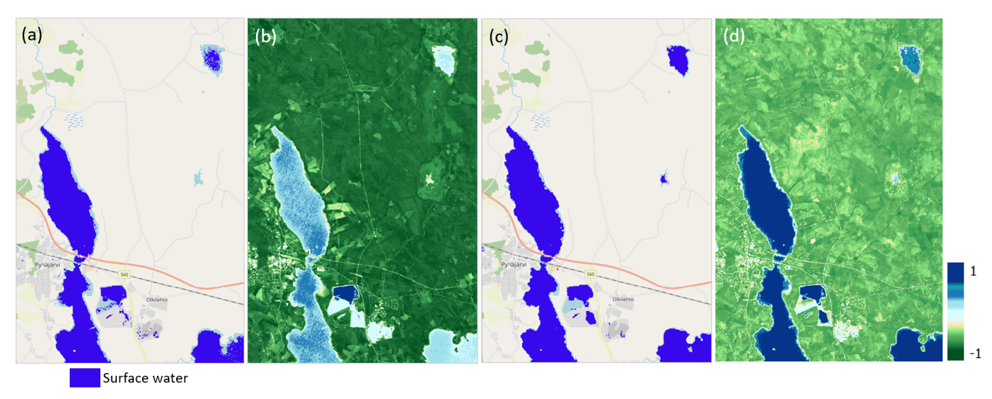
Figure 15.
Optical reference masks of surface water bodies, 28 August 2021: (a) NDWI water map; (b) NDWI spectral index; (c) MNDWI water map; (d) MNDWI spectral index. Basemap: OpenStreetMap Standard.
Figure 15.
Optical reference masks of surface water bodies, 28 August 2021: (a) NDWI water map; (b) NDWI spectral index; (c) MNDWI water map; (d) MNDWI spectral index. Basemap: OpenStreetMap Standard.
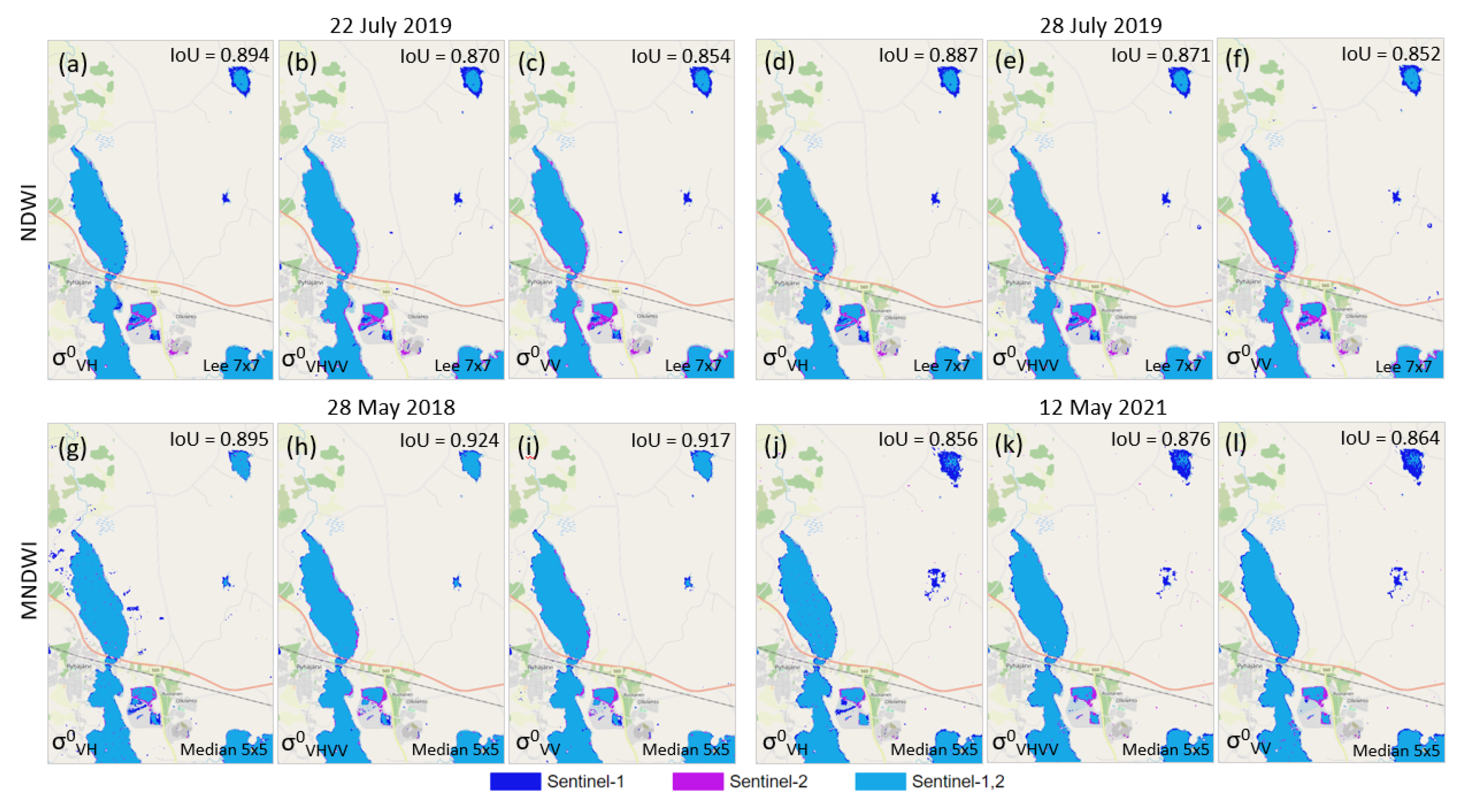
Figure 16.
Maps of surface water bodies based on SAR data , , and for the dates with the largest IoU discrepancies of water masks based on and : (a) 22 July 2019, NDWI, Lee 7 × 7, ; (b) 22 July 2019, NDWI, Lee 7 × 7, ; (c) 22 July 2019, NDWI, Lee 7 × 7, ; (d) 28 July 2019, NDWI, Lee 7 × 7, ; (e) 28 July 2019, NDWI, Lee 7 × 7, ; (f) 28 July 2019, NDWI, Lee 7 × 7, ; (g) 28 May 2018, MNDWI, Median 5 × 5, ; (h) 28 May 2018, MNDWI, Median 5 × 5, ; (i) 28 May 2018, MNDWI, Median 5 × 5, ; (j) 12 May 2021, MNDWI, Median 5 × 5, ; (k) 12 May 2021, MNDWI, Median 5 × 5, ; and (l) 12 May 2021, MNDWI, Median 5 × 5, . Basemap: OpenStreetMap Standard.
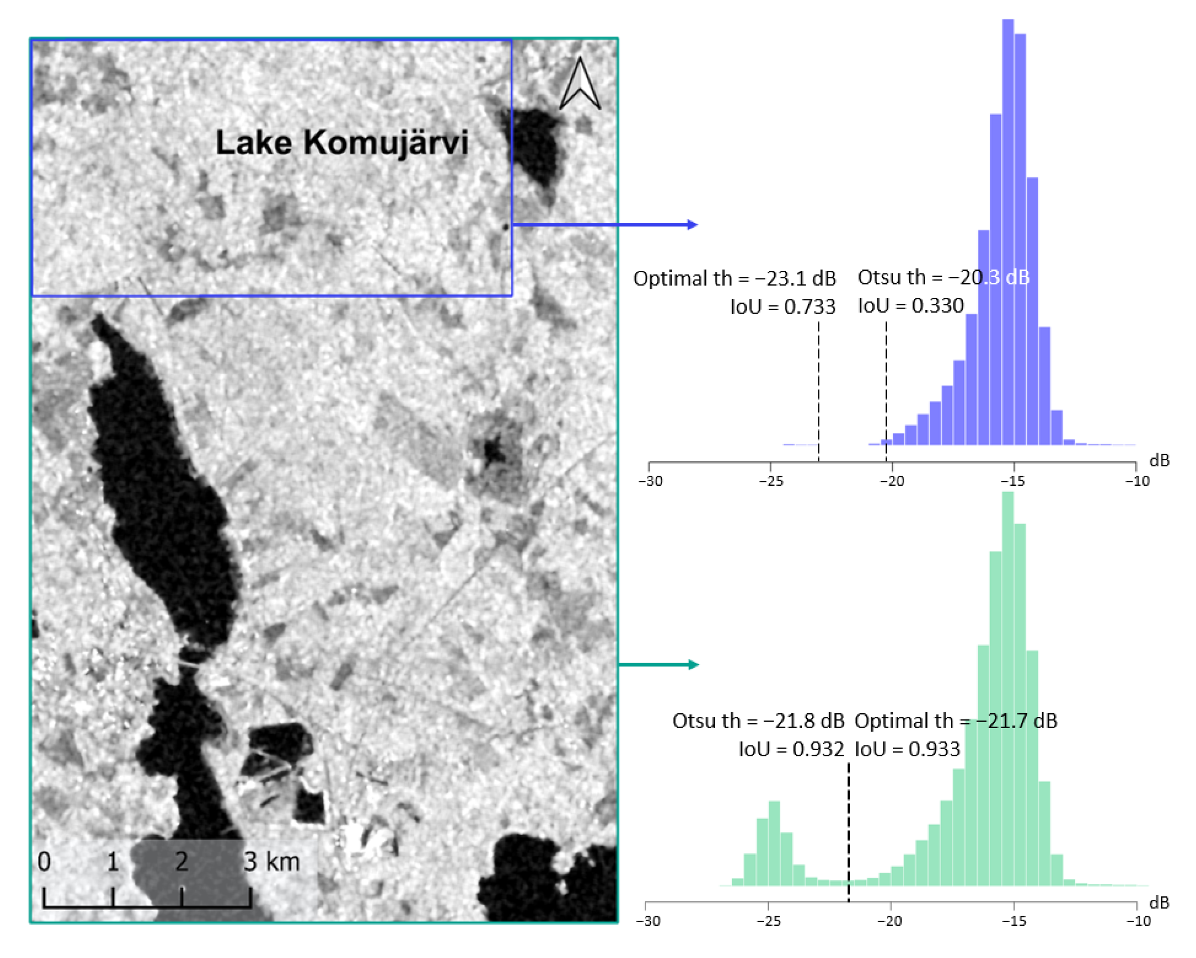
Figure 17.
Fragment of the study area— data with Lee Sigma 7 × 7 speckle filtering based on the MNDWI reference mask and histogram of the study area (green) and a small fragment (blue).
Figure 17.
Fragment of the study area— data with Lee Sigma 7 × 7 speckle filtering based on the MNDWI reference mask and histogram of the study area (green) and a small fragment (blue).
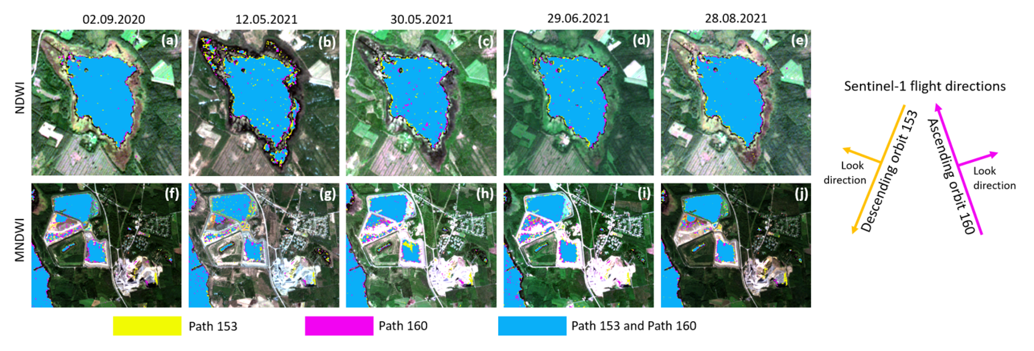
Figure 18.
Different-time SAR mask maps of surface water bodies based on data from two orbits for Lake Lohvanjärvi (a–e) and the Pyhäsalmi mine area (f–j): (a,f) 02 September 2020; (b,g) 12 May 2021; (c,h) 30 May 2021; (d,i) 29 June 2021; (e,j) 28 August 2021. Basemap: Sentinel-2 RGB (band-4, band-3, band-2).
Table 1.
Sentinel-1 and Sentinel-2 images acquisition dates and time.
Table 1.
Sentinel-1 and Sentinel-2 images acquisition dates and time.
| Sentinel-1 | Sentinel-2 |
|---|
| Date | Time | Date | Time |
| Path 153 | Path 160 |
| 28 August 2021 | 04:41:12 | 15:57:48 | 28 August 2021 | 10:02:50 |
| 23 July 2021 | 04:41:10 | 15:57:46 | 26 July 2021 | 09:52:55 |
| 29 June 2021 | 04:41:09 | 15:57:45 | 29 June 2021 | 10:02:50 |
| 11 June 2021 | 04:40:30 | 15:57:11 | 11 June 2021 | 09:52:53 |
| 30 May 2021 | 04:40:22 | 15:57:10 | 30 May 2021 | 10:02:49 |
| 12 May 2021 | 04:41:06 | 15:57:42 | 12 May 2021 | 09:52:50 |
| 02 September 2020 | 04:41:07 | 15:57:43 | 02 September 2020 | 10:02:53 |
| 15 August 2020 | 04:40:21 | 15:57:09 | 15 August 2020 | 09:52:55 |
| 16 June 2020 | 04:40:16 | 15:57:05 | 14 June 2020 | 10:02:55 |
| 23 May 2020 | 04:40:16 | 15:57:04 | 22 May 2020 | 09:52:57 |
| 28 July 2019 | 04:40:13 | 15:57:01 | 25 July 2019 | 10:02:57 |
| 22 July 2019 | 04:40:56 | 15:57:33 | 25 July 2019 | 10:02:57 |
| 23 May 2019 | 04:40:54 | 15:57:29 | 18 May 2019 | 09:52:55 |
| 15 July 2018 | 04:40:51 | 15:57:26 | 12 July 2018 | 09:50:30 |
| 03 July 2018 | 04:40:50 | 15:57:25 | 02 July 2018 | 09:50:30 |
| 28 May 2018 | 04:40:48 | 15:57:23 | 31 May 2018 | 10:00:23 |
Table 2.
Tables of median IoU similarity values for all combinations of speckle filtering parameters.
Table 2.
Tables of median IoU similarity values for all combinations of speckle filtering parameters.
| Path 153 |
|---|
| NDWI | MNDWI |
| | | | | |
| Sf 1 | IoU | Sf | IoU | Sf | IoU | Sf | IoU | Sf | IoU | Sf | IoU |
| L7 2 | 0.879 | M7 3 | 0.876 | M7 | 0.882 | M7 | 0.908 | LS7 4 | 0.883 | M7 | 0.894 |
| LS7 | 0.879 | LS7 | 0.874 | LS7 | 0.881 | LS7 | 0.906 | M7 | 0.882 | LS7 | 0.893 |
| GM7 5 | 0.876 | LS5 | 0.869 | M5 | 0.881 | L7 | 0.905 | LS5 | 0.876 | LS5 | 0.890 |
| M7 | 0.876 | M5 | 0.869 | LS5 | 0.880 | GM7 | 0.902 | M5 | 0.874 | M5 | 0.889 |
| L5 | 0.871 | RL 6 | 0.861 | RL | 0.878 | L5 | 0.901 | L5 | 0.870 | L5 | 0.886 |
| LS5 | 0.870 | L5 | 0.859 | M3 | 0.875 | LS5 | 0.901 | RL | 0.870 | L3 | 0.885 |
| GM5 | 0.870 | GM5 | 0.857 | L3 | 0.875 | GM5 | 0.899 | GM5 | 0.869 | GM3 | 0.885 |
| M5 | 0.865 | L7 | 0.853 | GM3 | 0.874 | M5 | 0.896 | GM7 | 0.867 | GM5 | 0.885 |
| L3 | 0.846 | L3 | 0.851 | L5 | 0.874 | RL | 0.880 | L7 | 0.866 | GM7 | 0.882 |
| GM3 | 0.845 | GM3 | 0.850 | GM5 | 0.872 | L3 | 0.879 | M3 | 0.865 | L7 | 0.881 |
| RL | 0.845 | GM7 | 0.850 | L7 | 0.871 | GM3 | 0.878 | L3 | 0.864 | RL | 0.881 |
| M3 | 0.837 | M3 | 0.849 | GM7 | 0.869 | M3 | 0.869 | GM3 | 0.863 | M3 | 0.880 |
| None | 0.775 | None | 0.811 | None | 0.854 | None | 0.805 | None | 0.832 | None | 0.868 |
| SD 7 | 0.029 | SD | 0.017 | SD | 0.007 | SD | 0.028 | SD | 0.013 | SD | 0.007 |
| LS7 | 0.887 | M7 | 0.878 | LS7 | 0.887 | M7 | 0.905 | M7 | 0.890 | M7 | 0.897 |
| L7 | 0.885 | LS7 | 0.877 | M7 | 0.887 | LS7 | 0.904 | LS7 | 0.888 | LS7 | 0.894 |
| M7 | 0.885 | M5 | 0.876 | M5 | 0.886 | L7 | 0.903 | LS5 | 0.883 | LS5 | 0.892 |
| L5 | 0.882 | LS5 | 0.876 | LS5 | 0.886 | GM7 | 0.900 | M5 | 0.882 | M5 | 0.892 |
| GM7 | 0.881 | RL | 0.874 | RL | 0.884 | L5 | 0.900 | L5 | 0.879 | RL | 0.890 |
| LS5 | 0.881 | L3 | 0.869 | M3 | 0.883 | LS5 | 0.900 | GM5 | 0.878 | L5 | 0.890 |
| GM5 | 0.879 | GM3 | 0.869 | L3 | 0.882 | GM5 | 0.898 | RL | 0.876 | GM5 | 0.889 |
| M5 | 0.876 | L5 | 0.868 | GM3 | 0.881 | M5 | 0.898 | L7 | 0.873 | GM7 | 0.887 |
| L3 | 0.864 | M3 | 0.868 | L5 | 0.881 | RL | 0.892 | L3 | 0.872 | L7 | 0.887 |
| GM3 | 0.864 | GM5 | 0.867 | GM5 | 0.880 | L3 | 0.889 | GM3 | 0.871 | GM3 | 0.886 |
| RL | 0.860 | L7 | 0.864 | L7 | 0.879 | GM3 | 0.888 | GM7 | 0.871 | L3 | 0.886 |
| M3 | 0.858 | GM7 | 0.861 | GM7 | 0.877 | M3 | 0.884 | M3 | 0.867 | M3 | 0.885 |
| None | 0.821 | None | 0.828 | None | 0.868 | None | 0.835 | None | 0.836 | None | 0.874 |
| SD | 0.018 | SD | 0.013 | SD | 0.005 | SD | 0.018 | SD | 0.013 | SD | 0.006 |
Table 3.
Quantitative plateau characteristics for all filters, polarization, and reference masks, 22 July 2019.
Table 3.
Quantitative plateau characteristics for all filters, polarization, and reference masks, 22 July 2019.
| NDWI | MNDWI |
|---|
| Filter | Start 1 | End 2 | PW 3 | IoU | | Filter | Start | End | PW | IoU | |
| L7 4 | −14.8 | −19.3 | 4.5 | 0.854 | | GM7 5 | −14.8 | −19.2 | 4.4 | 0.836 | |
| GM7 | −14.9 | −19.3 | 4.4 | 0.852 | | L7 | −14.7 | −19.1 | 4.4 | 0.837 | |
| LS7 6 | −15.0 | −19.4 | 4.4 | 0.876 | | LS7 | −14.9 | −19.2 | 4.3 | 0.866 | |
| GM7 | −17.1 | −21.5 | 4.4 | 0.869 | | GM5 | −15.1 | −19.3 | 4.2 | 0.845 | |
| L7 | −17.1 | −21.5 | 4.4 | 0.870 | | M7 7 | −15.3 | −19.5 | 4.2 | 0.871 | |
| LS7 | −17.3 | −21.7 | 4.4 | 0.885 | | GM7 | −17.0 | −21.2 | 4.2 | 0.857 | |
| M7 | −15.4 | −19.7 | 4.3 | 0.878 | | L5 | −15.1 | −19.2 | 4.1 | 0.846 | |
| M7 | −17.7 | −22.0 | 4.3 | 0.886 | | LS5 | −15.1 | −19.2 | 4.1 | 0.861 | |
| GM5 | −15.2 | −19.4 | 4.2 | 0.860 | | GM5 | −17.3 | −21.4 | 4.1 | 0.864 | |
| L5 | −15.2 | −19.4 | 4.2 | 0.862 | | M7 | −17.5 | −21.6 | 4.1 | 0.886 | |
| GM5 | −17.4 | −21.6 | 4.2 | 0.875 | | L5 | −17.3 | −21.4 | 4.1 | 0.865 | |
| L5 | −17.4 | −21.6 | 4.2 | 0.876 | | L7 | −17.0 | −21.1 | 4.1 | 0.857 | |
| LS5 | −17.5 | −21.7 | 4.2 | 0.884 | | LS7 | −17.2 | −21.3 | 4.1 | 0.880 | |
| LS5 | −15.3 | −19.4 | 4.1 | 0.873 | | M5 | −15.5 | −19.5 | 4.0 | 0.867 | |
| M5 | −17.9 | −21.9 | 4.0 | 0.885 | | M5 | −17.7 | −21.7 | 4.0 | 0.881 | |
| M5 | −15.7 | −19.6 | 3.9 | 0.875 | | LS5 | −17.4 | −21.4 | 4.0 | 0.877 | |
| RL 8 | −15.7 | −19.5 | 3.8 | 0.874 | | RL | −17.7 | −21.5 | 3.8 | 0.880 | |
| RL | −17.9 | −21.7 | 3.8 | 0.884 | | RL | −15.6 | −19.3 | 3.7 | 0.865 | |
| GM3 | −15.7 | −19.3 | 3.6 | 0.864 | | GM3 | −17.7 | −21.4 | 3.7 | 0.869 | |
| L3 | −15.7 | −19.3 | 3.6 | 0.865 | | L3 | −17.7 | −21.4 | 3.7 | 0.870 | |
| GM3 | −17.9 | −21.5 | 3.6 | 0.878 | | GM3 | −15.6 | −19.2 | 3.6 | 0.852 | |
| L3 | −17.9 | −21.5 | 3.6 | 0.879 | | L3 | −15.6 | −19.2 | 3.6 | 0.852 | |
| M3 | −16.0 | −19.5 | 3.5 | 0.867 | | M3 | −15.9 | −19.4 | 3.5 | 0.857 | |
| M3 | −18.2 | −21.7 | 3.5 | 0.881 | | M3 | −18.0 | −21.5 | 3.5 | 0.876 | |
| L7 | −20.6 | −23.8 | 3.2 | 0.894 | | GM7 | −20.2 | −23.3 | 3.1 | 0.919 | |
| G7 | −20.7 | −23.8 | 3.1 | 0.892 | | L7 | −20.2 | −23.3 | 3.1 | 0.920 | |
| LS7 | −20.8 | −23.8 | 3.0 | 0.897 | | LS7 | −20.3 | −23.4 | 3.1 | 0.924 | |
| | | | | | | M7 | −20.7 | −23.7 | 3.0 | 0.926 | |
Table 4.
Comparison of the accuracy of SAR water masks generated by the Otsu method and the proposed method based on the optimal thresholds of the reference date and the averaged optimal thresholds for all dates in 2018–2020.
Table 4.
Comparison of the accuracy of SAR water masks generated by the Otsu method and the proposed method based on the optimal thresholds of the reference date and the averaged optimal thresholds for all dates in 2018–2020.
| 29 June 2021 1 | Otsu IoU | Reference Date—11 June 2021 | All Dates 2018–2020 |
|---|
| Th 2 | Opt. IoU 3 | IoU
4 | Th | Opt. IoU | IoU |
|---|
| Lee 5 × 5 | 0.911 | −22.5 | 0.896 | 0.015 | −22.7 | 0.913 | −0.002 |
| Lee 7 × 7 | 0.916 | −22.2 | 0.911 | 0.005 | −22.5 | 0.917 | −0.001 |
| Lee Sigma 5 × 5 | 0.911 | −22.4 | 0.890 | 0.021 | −22.7 | 0.914 | −0.003 |
| Lee Sigma 7 × 7 | 0.914 | −22.4 | 0.902 | 0.012 | −22.7 | 0.920 | −0.006 |
| Median 5 × 5 | 0.899 | −22.7 | 0.887 | 0.012 | −23.0 | 0.908 | −0.009 |
| Median 7 × 7 | 0.902 | −23.0 | 0.899 | 0.003 | −23.1 | 0.919 | −0.017 |
| 28 August 2021 | OtsuIoU | Reference Date—11 June 2021 | All Dates 2018–2020 |
| Th | Opt.IoU | IoU | Th | Opt.IoU | IoU |
| Lee 5 × 5 | 0.924 | −22.2 | 0.902 | 0.022 | −22.7 | 0.918 | 0.006 |
| Lee 7 × 7 | 0.919 | −22.3 | 0.904 | 0.015 | −22.5 | 0.915 | 0.004 |
| Lee Sigma 5 × 5 | 0.928 | −22.2 | 0.900 | 0.028 | −22.7 | 0.922 | 0.006 |
| Lee Sigma 7 × 7 | 0.932 | −21.8 | 0.902 | 0.030 | −22.7 | 0.923 | 0.009 |
| Median 5 × 5 | 0.928 | −22.3 | 0.901 | 0.027 | −22.7 | 0.922 | 0.006 |
| Median 7 × 7 | 0.933 | −22.3 | 0.904 | 0.029 | −23.1 | 0.926 | 0.007 |
Table 5.
threshold values and IoU metrics of SAR and optical water masks similarity for path = 160, path = 153, and all observation dates.
Table 5.
threshold values and IoU metrics of SAR and optical water masks similarity for path = 160, path = 153, and all observation dates.
| SAR Date | NDWI | MNDWI |
|---|
| Similarity (IoU) | Threshold (dB) | Similarity (IoU) | Threshold (dB) |
|---|
| 153 1 | 160 1 | 153 | 160 | 153 | 160 | 153 | 160 |
|---|
| 28 August 2021 | 0.880 | 0.884 | −22.7 | −24.6 | 0.926 | 0.936 | −21.3 | −22.7 |
| 23 July 2021 | 0.796 | 0.802 | −23.1 | −24.1 | 0.916 | 0.900 | −21.2 | −21.8 |
| 29 June 2021 | 0.831 | 0.841 | −23.1 | −23.9 | 0.918 | 0.907 | −22.2 | −22.2 |
| 11 June 2021 | 0.899 | 0.901 | −23.4 | −23.7 | 0.904 | 0.895 | −23.0 | −23.1 |
| 30 May 2021 | 0.744 | 0.749 | −23.9 | −24.8 | 0.891 | 0.892 | −23.6 | −24.0 |
| 12 May 2021 | 0.905 | 0.907 | −22.1 | −23.2 | 0.884 | 0.891 | −22.7 | −23.9 |
| 02 September 2020 | 0.880 | 0.885 | −23.2 | −24.3 | 0.881 | 0.883 | −22.7 | −23.3 |
| 15 August 2020 | 0.874 | 0.879 | −23.6 | −24.6 | 0.906 | 0.912 | −22.5 | −23.3 |
| 16 June 2020 | 0.909 | 0.914 | −23.0 | −23.7 | 0.906 | 0.912 | −22.9 | −23.5 |
| 23 May 2020 | 0.827 | 0.827 | −23.2 | −24.2 | 0.906 | 0.910 | −23.5 | −24.4 |
| 28 July 2019 | 0.887 | 0.894 | −22.6 | −23.1 | 0.896 | 0.906 | −22.1 | −22.4 |
| 22 July 2019 | 0.894 | 0.899 | −22.5 | −23.4 | 0.920 | 0.922 | −21.6 | −21.5 |
| 23 May 2019 | 0.853 | 0.858 | −23.2 | −24.7 | 0.873 | 0.883 | −23.3 | −24.8 |
| 15 July 2018 | 0.892 | 0.893 | −24.2 | −23.2 | 0.903 | 0.898 | −22.0 | −22.4 |
| 03 July 2018 | 0.878 | 0.887 | −22.7 | −24.0 | 0.881 | 0.885 | −21.8 | −22.8 |
| 28 May 2018 | 0.797 | 0.811 | −23.2 | −24.0 | 0.912 | 0.924 | −22.9 | −23.6 |


