1. Introduction
Over the past few decades, natural disasters have seriously damaged both natural and man-made settings. One of the riskiest situations involving water is flooding, which is primarily responsible for fatalities, damage to infrastructure, and financial losses. Because flood events are occurring more frequently, with larger sizes, and more intensely, there is currently a growing global awareness of the need to mitigate flood damage [
1]. The Diffusion Wave Equation (DWE) is an approximated shape of the shallow water equations (SWE) which is often used to model overland flows such as floods, dam breaks, and flows through vegetated areas. Diffusive shallow water (DSW) further simplifies the SWE by assuming that the horizontal momentum can be linked to the water height through an empirical formula, such as Manning’s [
2]. The hydraulic simulation models are crucial instruments for comprehending the hydraulic properties of river-system flow [
2].
The roughness coefficient (or Manning’s coefficient) is a significant hydraulic parameter, particularly in hydraulic modeling [
3,
4]. Specific values for the empirical parameters, such as Manning’s coefficient n, are frequently ambiguous due to the complexity of hydraulic engineering. The channel surface roughness, bed material, vegetation, channel alignment and irregularities, channel form and size, stage and discharge, suspended sediment load and bed sediment loads, etc., are all included in the roughness coefficient (Manning’s n) as an empirical parameter [
5]. Several past empirical formulas have been proposed for estimating the surface roughness (n) values in practical problems [
6].
Several researchers proposed several approaches for determining Manning’s roughness values n [
7,
8,
9]. Parhi calibrated and validated the value of the roughness coefficient (n) for the Mahanadi River in Odisha using the HEC-RAS model (India). In the calibration and verification, Parhi considered the floods of 2001 and 2003 [
10]. Additionally, Shamkhi and Attab investigated and calculated the value of n downstream of the Kut Barrage in Wasit, Iraq, using the HEC-RAS model [
11]. Using inversion techniques, Calo et al. calculated the distributed Manning’s coefficient directly from water height measurements. To do this, an inverse problem was created for calculating n using measurements of the water height obtained from sensors and infrared imaging [
2]. Using HEC-RAS software, Abbas et al. investigated the idea of a hydraulic model to calculate Manning’s coefficient n of the Tigris River along 3.5 km in the Maysan Governorate, southern Iraq [
3]. In flood inundation modeling and mapping, Papaioannou et al. examined the uncertainty caused by the roughness values on hydraulic models. The initial values of Manning’s n roughness coefficient are derived from field surveys and empirical formulas. To represent the estimated roughness values, a variety of theoretical probability distributions are fitted and evaluated for accuracy, and then flood inundation probability maps are produced using Monte Carlo simulations [
1].
Numerous sources of uncertainty impact the modeling of flood hydraulics (e.g., input data, model structure, model parameters). The most recent advancement in HEC-RAS software is the simulation of 2D unsteady flows in response to rain-on-grid model input, accounting for soil infiltration and flood routing parameters with spatial variation of roughness values. Water depth and velocity variability in floodplain and channel environments can be quantified using HEC-RAS 2D rain-on-grid simulations [
12,
13]. Manning’s roughness coefficient (n) is commonly used to represent surface roughness in distributed hydrologic models. Model parameter sensitivity studies identify runoff responses sensitive to Manning’s changes. Despite the availability of defined standard Manning’s values [
14], these standard values may result in inaccurate results if applied directly to 2D models [
15]. Recently, researchers concluded that by using increased roughness values compared to the standard with a low-resolution digital elevation model (DEM) and decreased roughness values compared to the standard with a high-resolution DEM, the 2D models perform better [
16,
17].
Several studies [
18,
19] showed how geospatial data resolution could affect the 2D model results. The ability of 2D flood models to generate reliable flood simulations is primarily determined by the quality of inputted topography and surface roughness data, as well as the level to which these data are captured in the computational mesh structure. These two key inputs to which 2D models exhibit high sensitivity are generally given in the digital elevation model (DEM) that represents the topography and Land-use/Land-cover (LULC) raster maps that are used to determine the roughness coefficient (Manning’s coefficient n), respectively [
20]. Therefore, more research is needed to understand how different land-use/land-cover data sources with assigned Manning’s roughness influence the 2D model accuracy [
21].
The Copernicus Global Land Service (CGLS) recently delivered a 100 m resolution land cover map that was generated by applying the vegetation sensor on the platform of the PROBA-V satellite [
22]. The data were divided into groups by comparing the land cover of testing sites with various available local datasets [
22,
23]. The main advantages of land-cover CGLS datasets are their high resolution (100 m) compared with other available land-cover datasets, but the main issue is that they can only be used on a national scale and they do not cover the regional scale [
24]. As an advancement from the legacy of the open-source Landsat, the National Aeronautics and Space Administration and U.S. Geological Survey (NASA/USGS) program provides a continuous space-based record of Earth’s land [
25]. Landsat data give us information essential for land cover and could be used easily to obtain land-use/land-cover maps at 10–30 m resolution [
26,
27,
28,
29]. In partnership with several federal agencies, the U.S. Geological Survey (USGS) has released five National Land Cover Database (NLCD) products over the last twenty years (1992–2016) [
30].
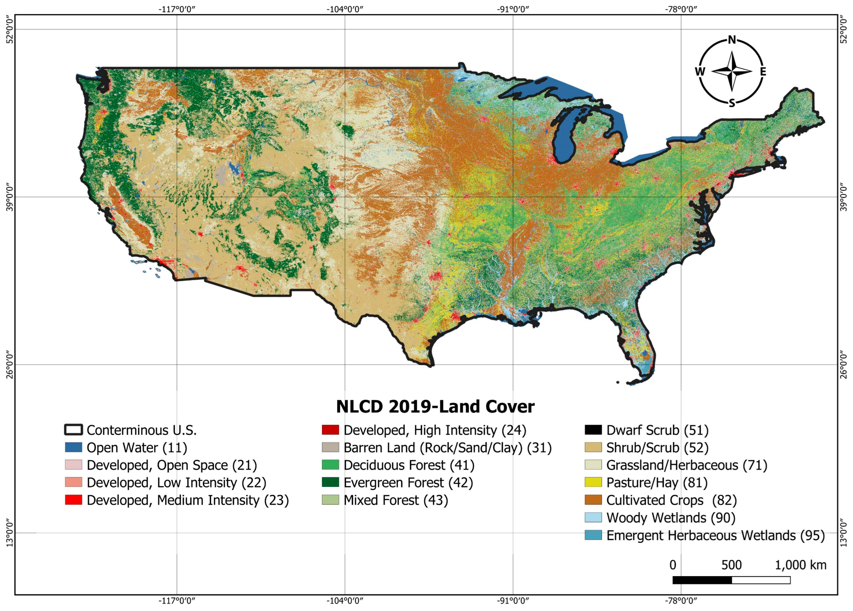
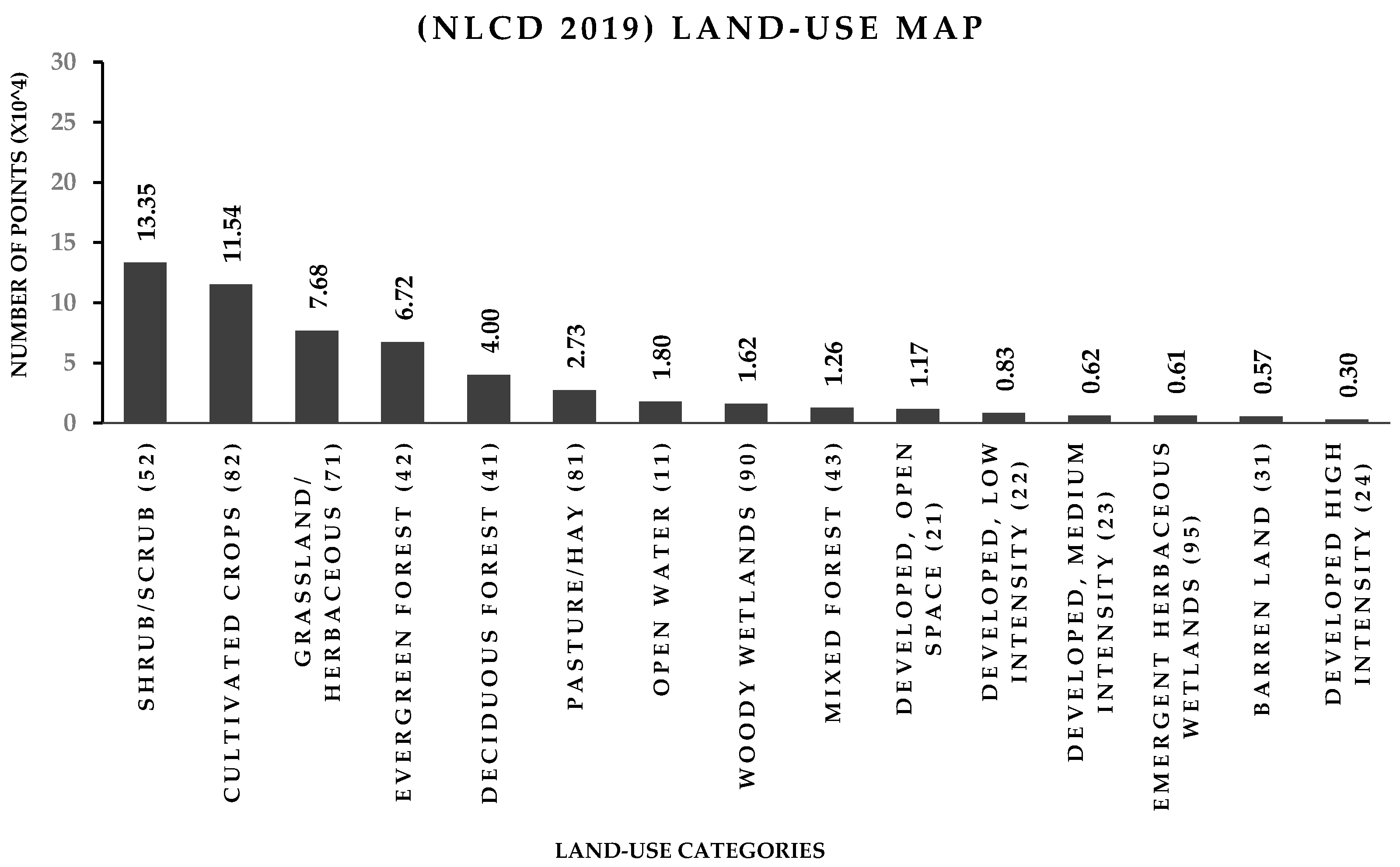
In July 2021, USGS generated and released a new version of NLCD with the resolution of 30 m Landsat-based products named NLCD 2019 [
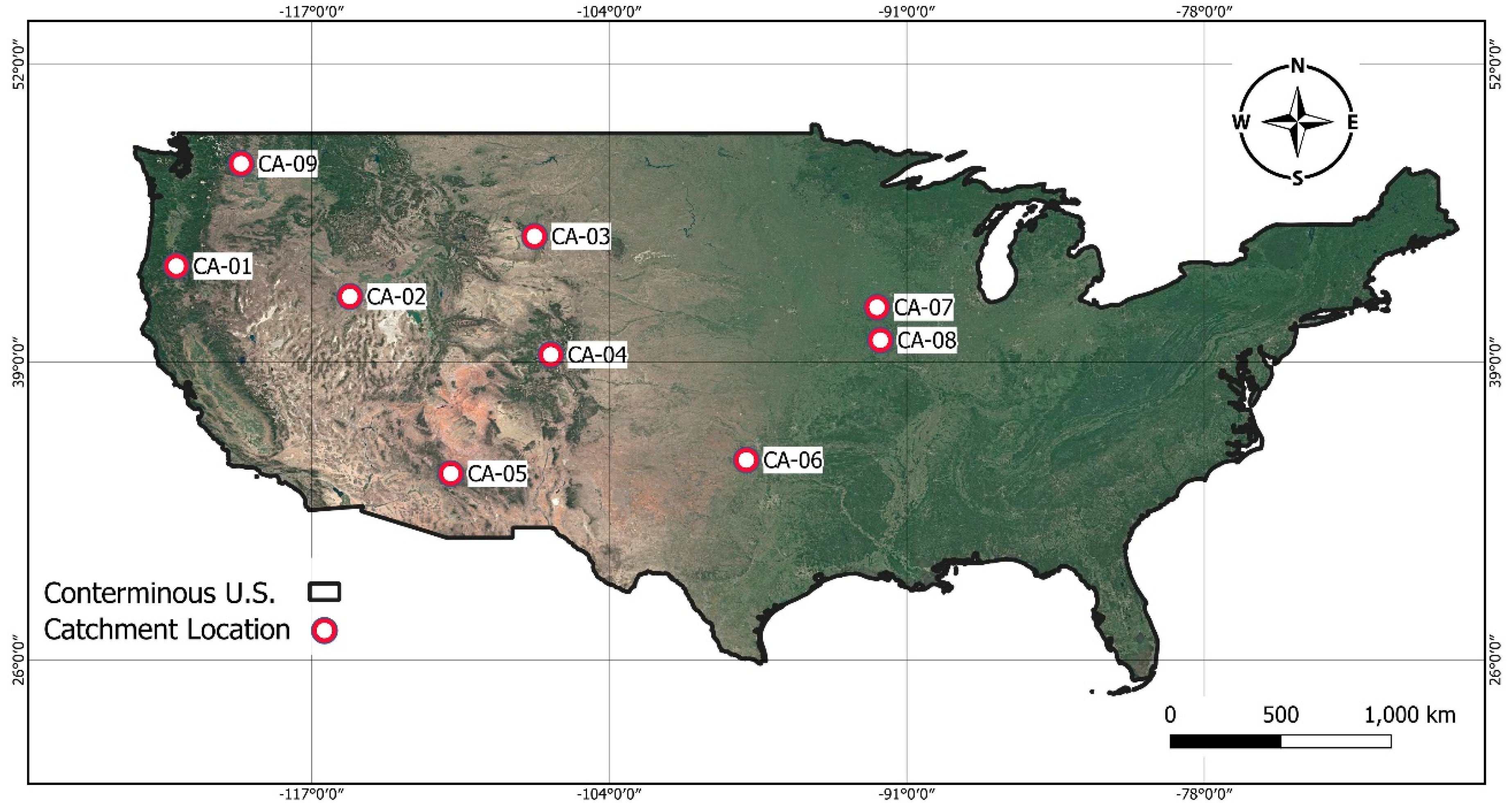
31]. The latest version of NLCD contains land-use/land-cover classes. This new version was tested at about twenty composite sites in the conterminous United States with an overall accuracy of 91% [
31]. The problem here is that NLCD 2019 map data are only available in the conterminous United States and has no global coverage [
32].
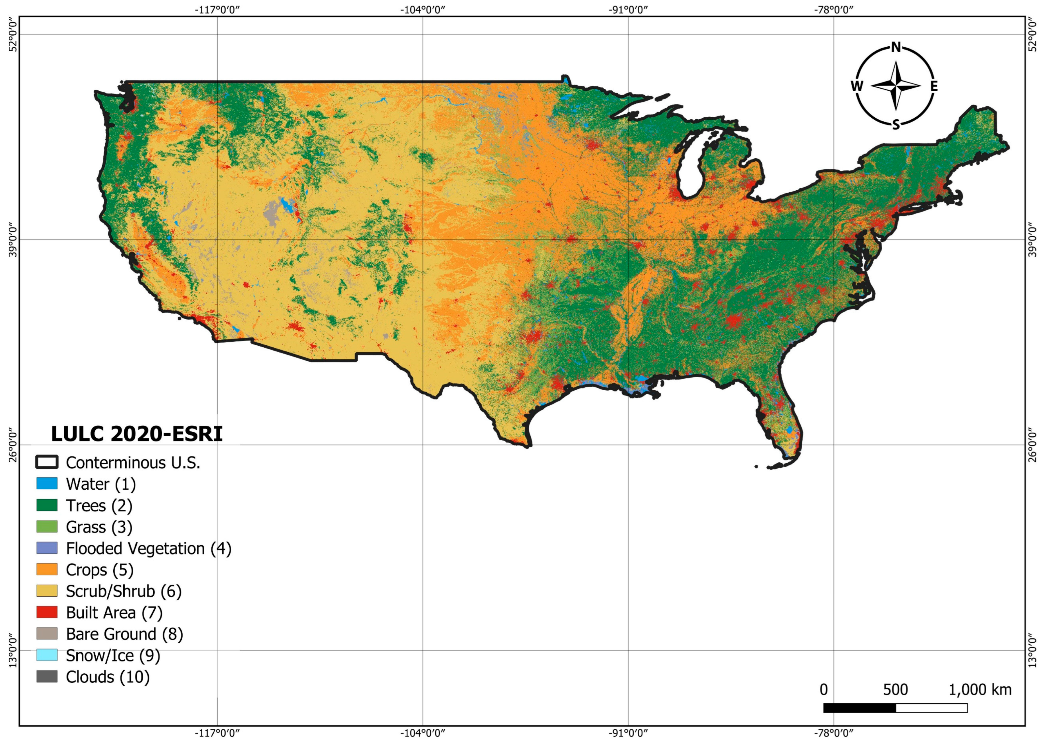
The Environmental Systems Research Institute (ESRI) in June 2021 released a new dataset called LULC 2020-ESRI using Artificial Intelligence of the European Space Agency (ESA) Sentinel-2 satellite with a resolution of 10 m [
27,
33]. The main advantage of this new dataset is that it can be used to represent global land-use and land-cover mapping at national and local scales. The main issue with LULC 2020-ESRI is that it is new data containing fewer classes of land use/land cover compared to NLCD data, and without associated ranges for Manning’s values per each class as in NLCD data, so its accuracy was not tested or evaluated [
33].
Recent studies discussed the accuracy of land-use/land-cover global maps corresponding to other local-scale ground observations [
34] or comparing them to global-scale land-use maps [
35]. The studies showed that the overall accuracy of global LULC 2020-ESRI was 75% compared to ground truth data of 250 m
2 resolution [
35], where the resolution of the ground data was very coarse to be confidently accepted as a reference layer. Moreover, there is a lack of testing of the effect of implementing the global LULC 2020 -ESRI data along with the roughness values in the 2D flood modeling applications.
Modelers typically use land-use/land-cover datasets for watershed simulations to assign appropriate Manning’s values based on the land-use or -cover class [
36]. Therefore, HEC-RAS developers [
5] released a reference to Manning’s roughness values corresponding to the NLCD dataset classes to be used with 2D flood modeling to identify the land use/landcover within the United States, but there are no reference Manning’s roughness values corresponding to the LULC 2020-ESRI dataset.
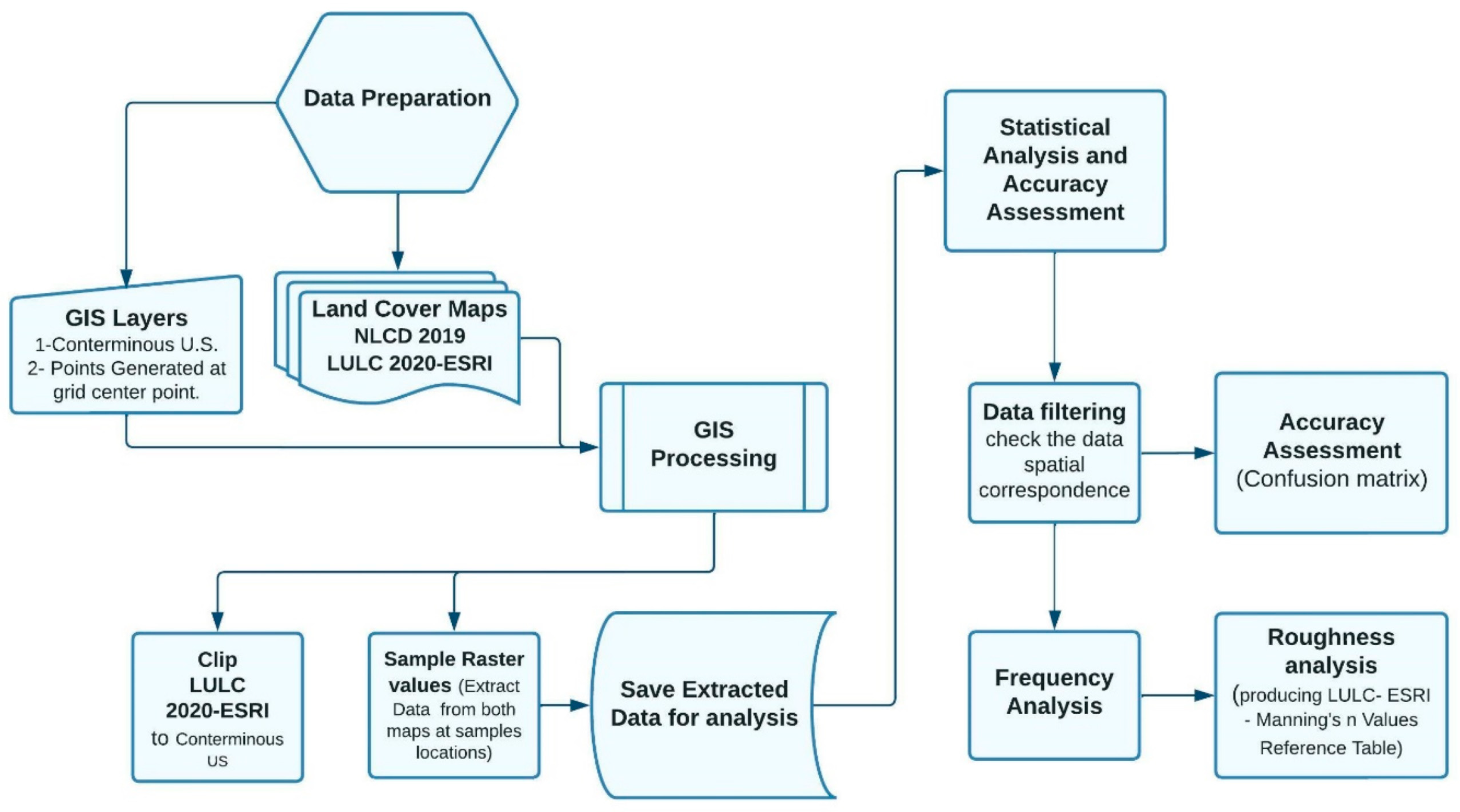
There are two main purposes of this research. The first is to assess the accuracy of the LULC 2020-ESRI data compared to the NLCD 2019 data given the availability of recommended Manning’s roughness values for NLCD by the HEC-RAS developers [
5]. The second is to produce reference Manning’s roughness (n) maps for each topology in the global land-use maps, LULC 2020-ESRI. The generated proposed Manning’s roughness values were based on the recommended Manning’s roughness values proposed by HEC-RAS developers [
5] for the NLCD 2019 (used as a reference) based on the standard values in Chow’s book (Chow, 1959) [
14].
This research is considered a first preliminary step toward using such global data as LULC 2020-ESRI in 2D distributed models in any spot on the globe efficiently and accurately by developing a standard reference Manning’s roughness value for each land-use/land-cover class in the dataset.
4. Discussion
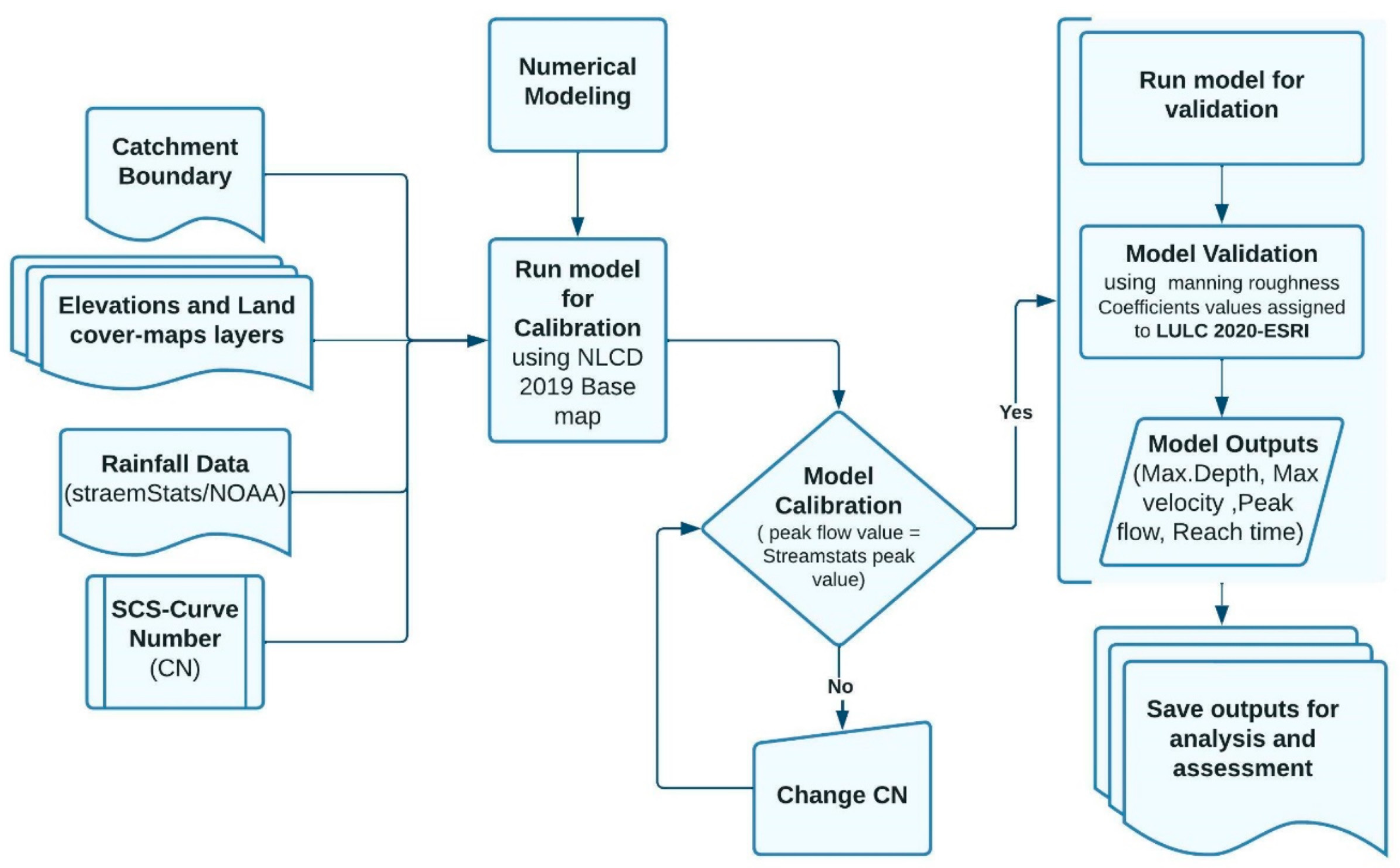
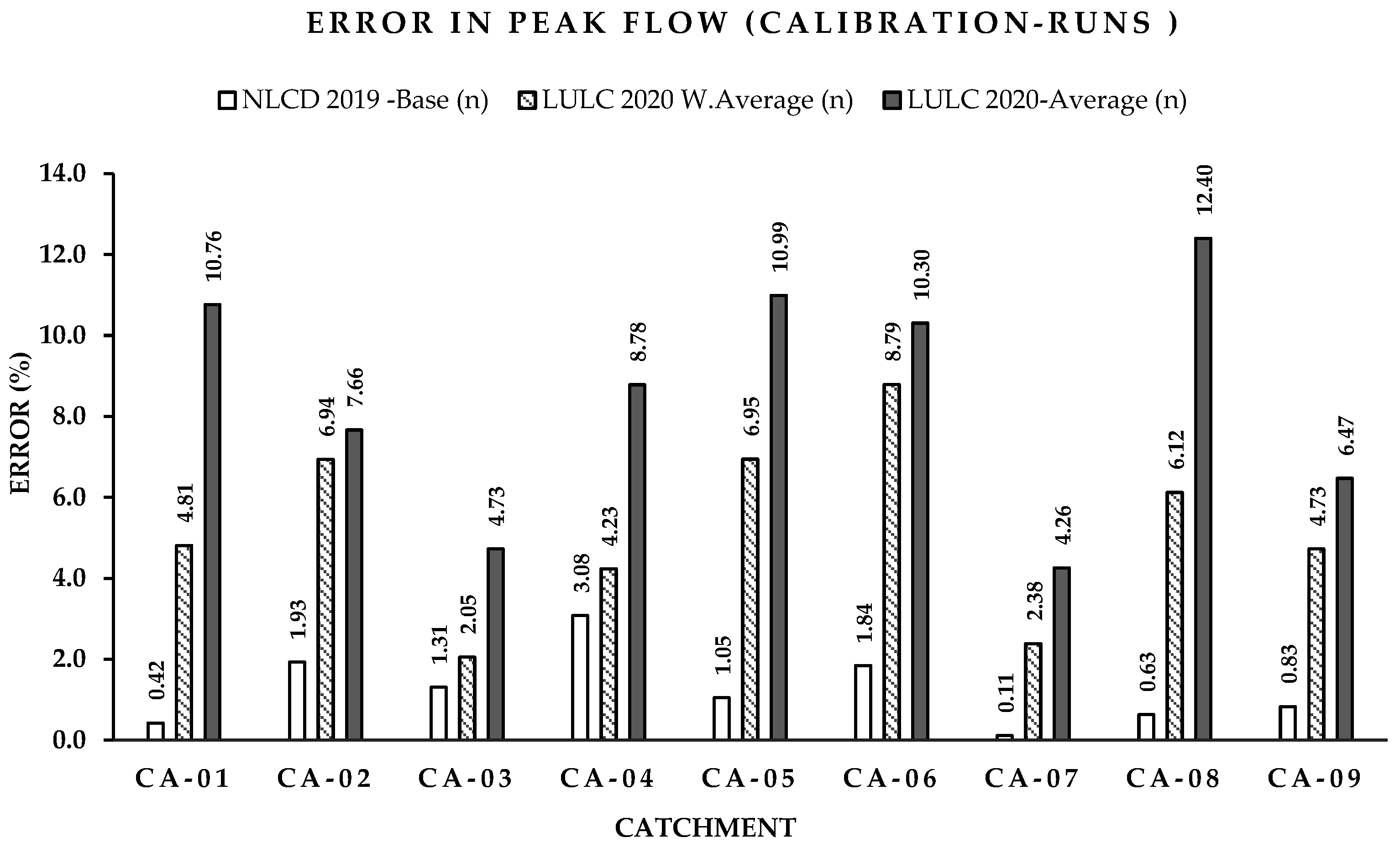
Based on the statistical analysis results, it is obvious that the data from NLCD 2019 is denser and more accurate where it can catch the observed peak flow with an error ranging from 0.42% to a maximum of 3.08% for calibration and validation processes, respectively. These error rates were lower in the long return period (100-year validation process) than for the short return period (2-years calibration process) (
Table 8 and
Table 9). However, the NLCD 2019 is only available for the conterminous U.S. and it cannot be used for global coverage. Due to the main advantage of global coverage for the LULC 2020-ESRI map, there was a need to make full use of the NLCD 2019 dataset to enhance the accuracy and propose Manning’s roughness values for the LULC 2020-ESRI dataset.
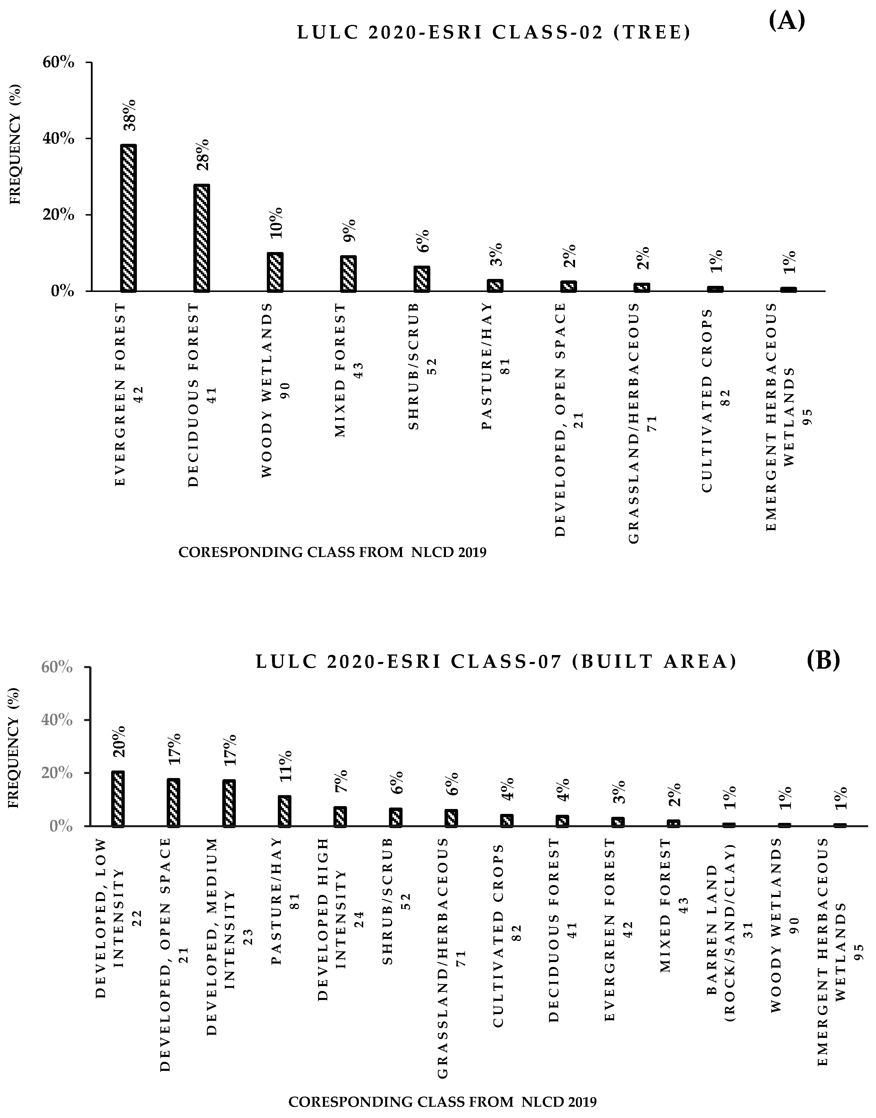
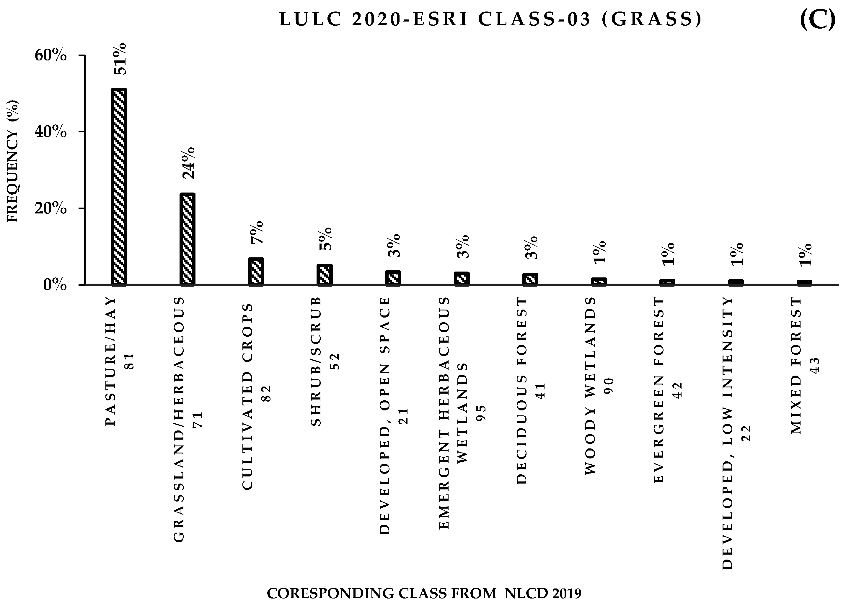
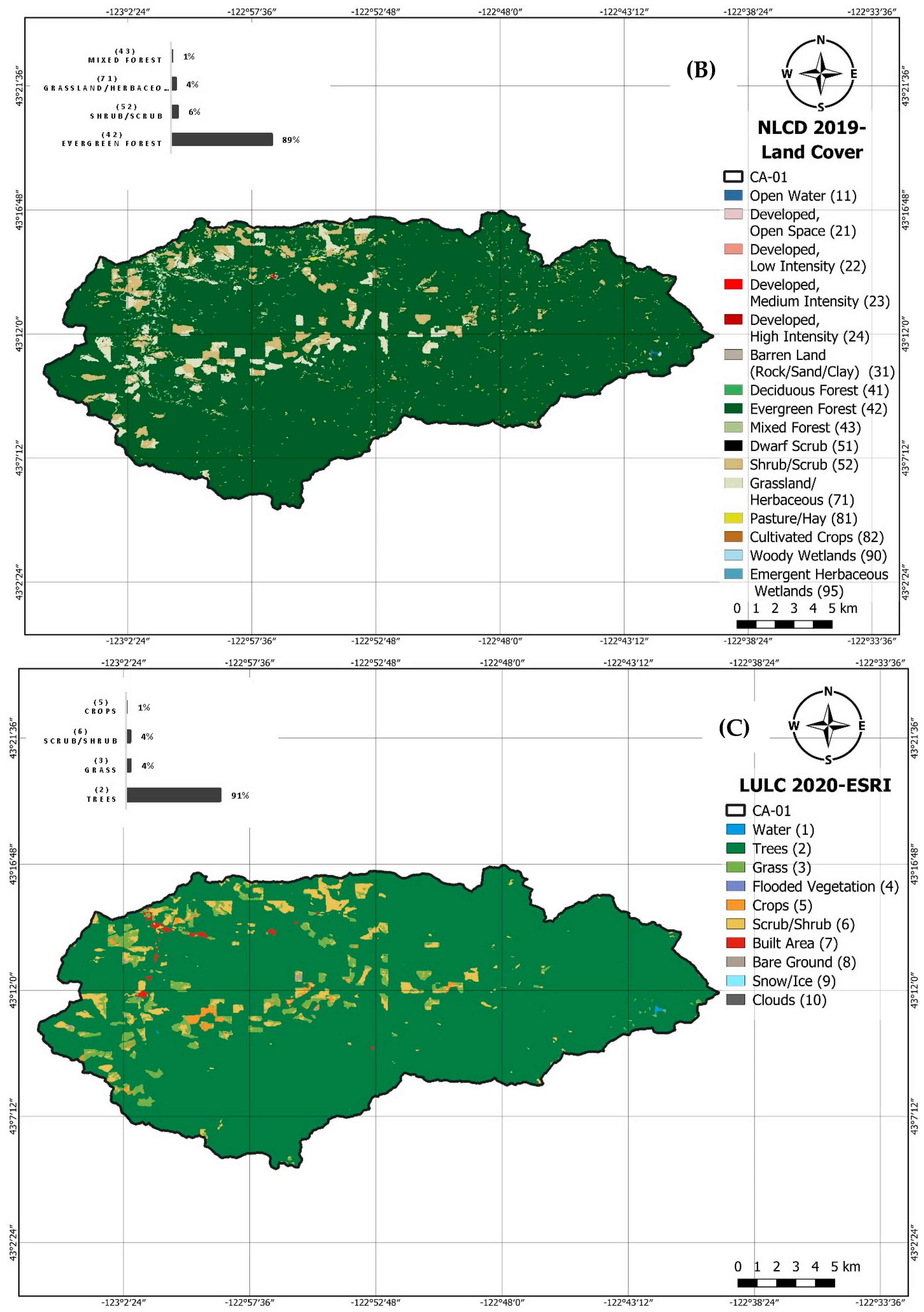
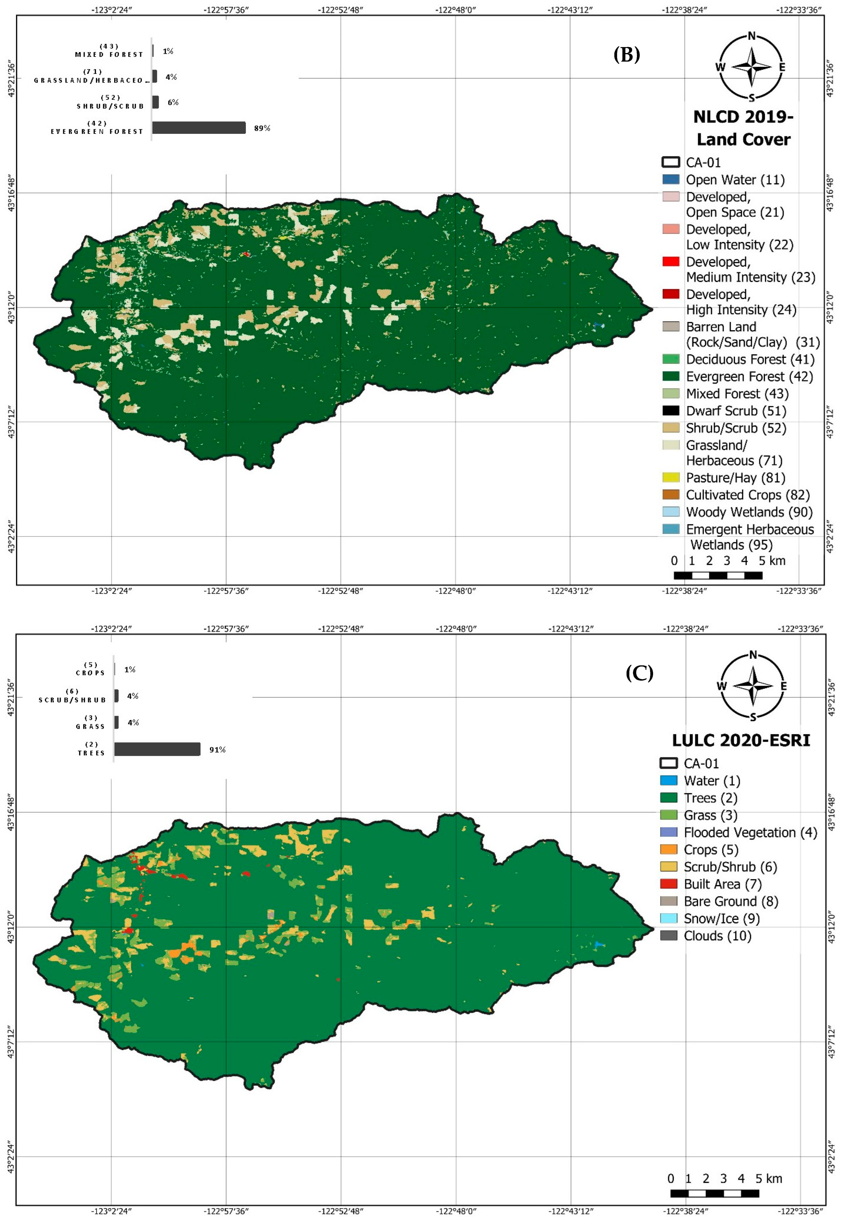
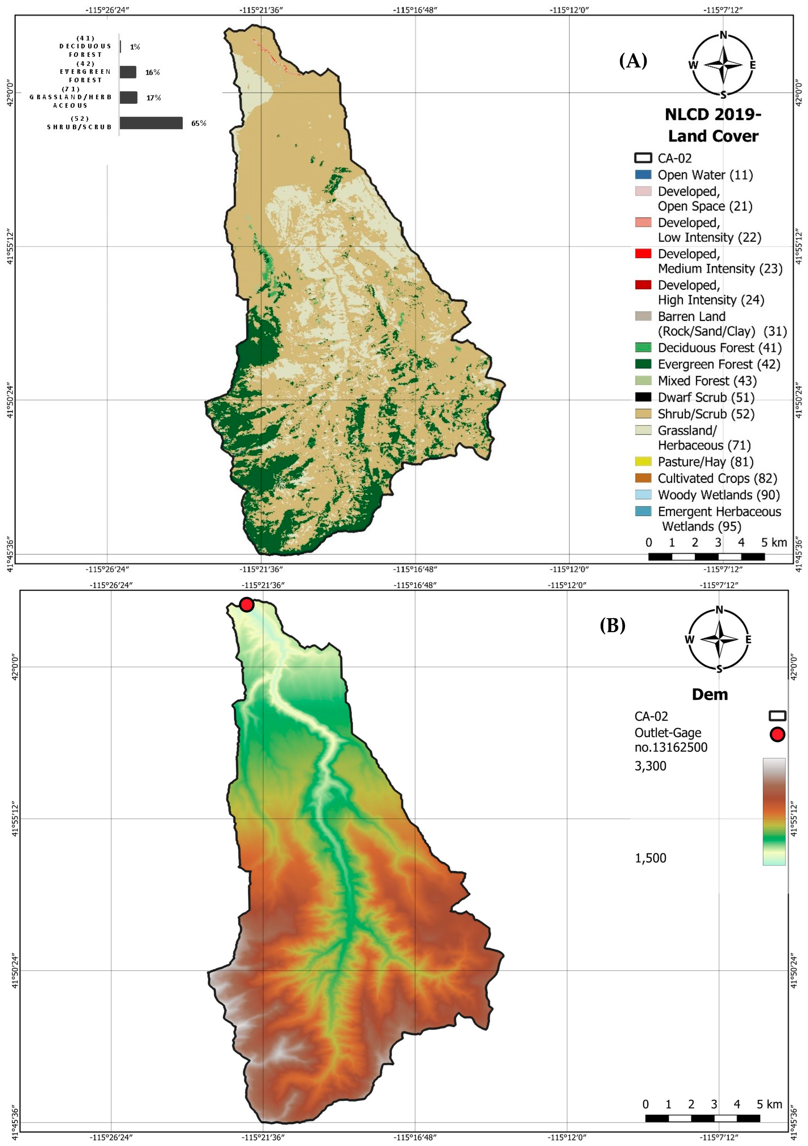
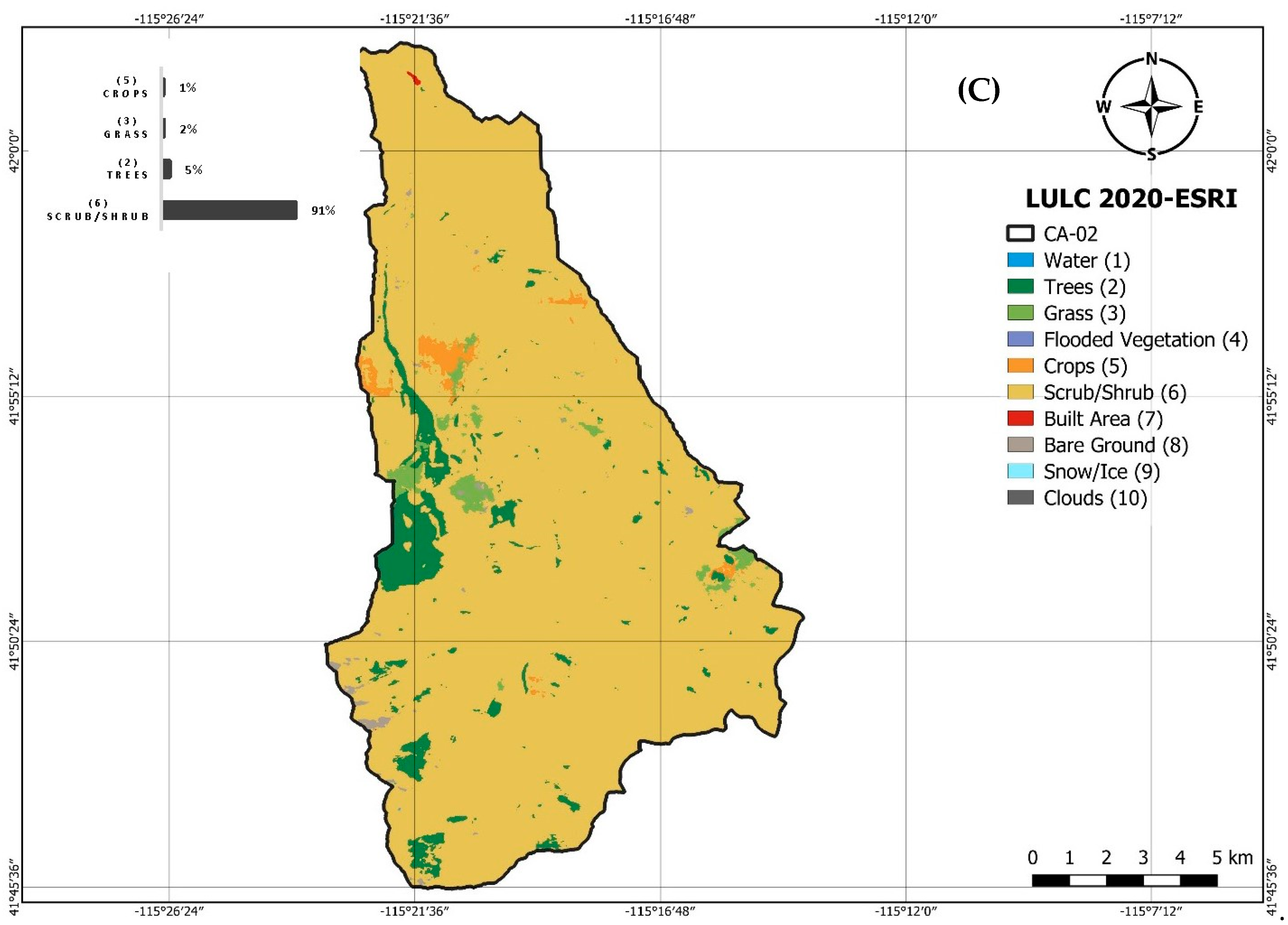
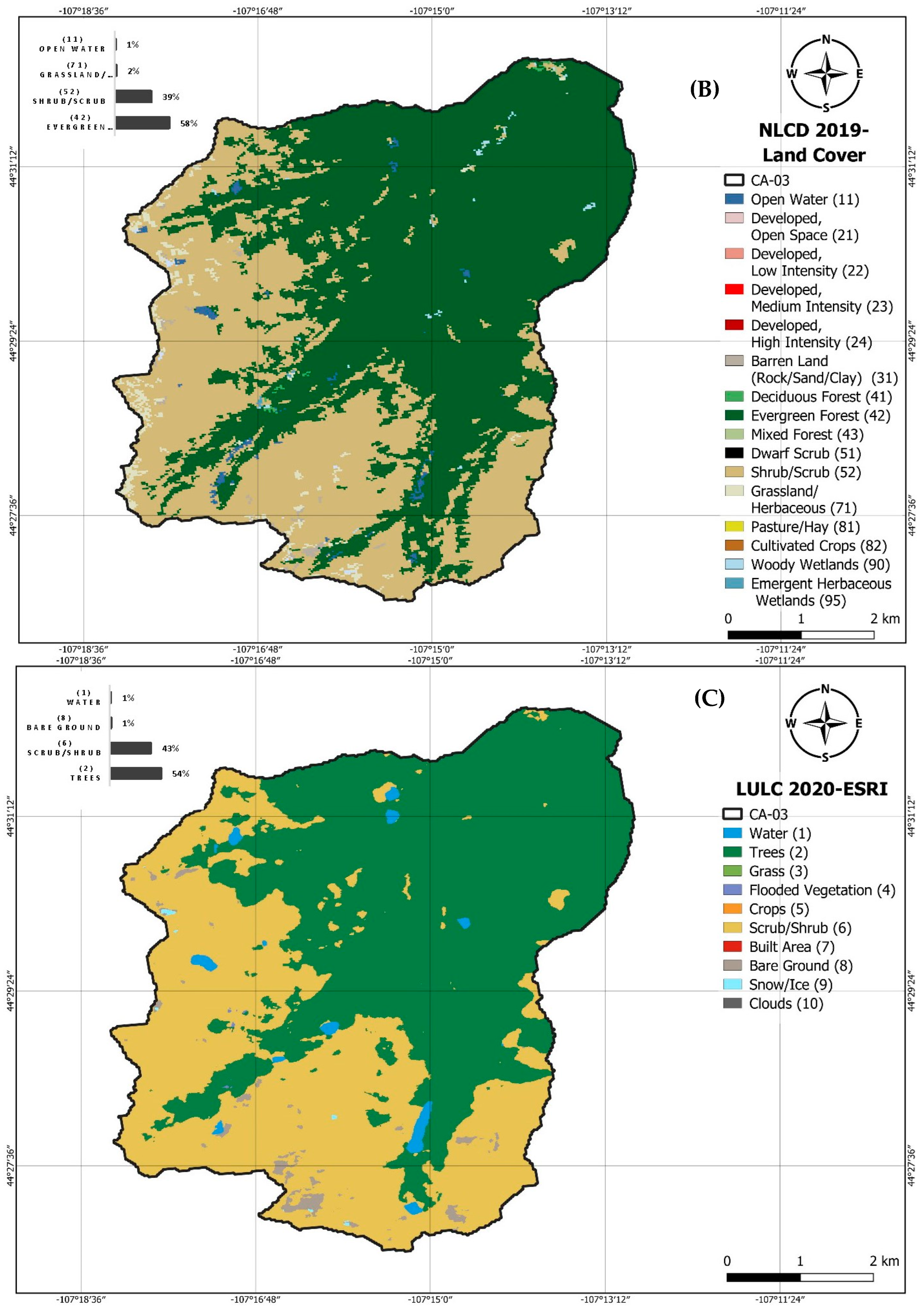
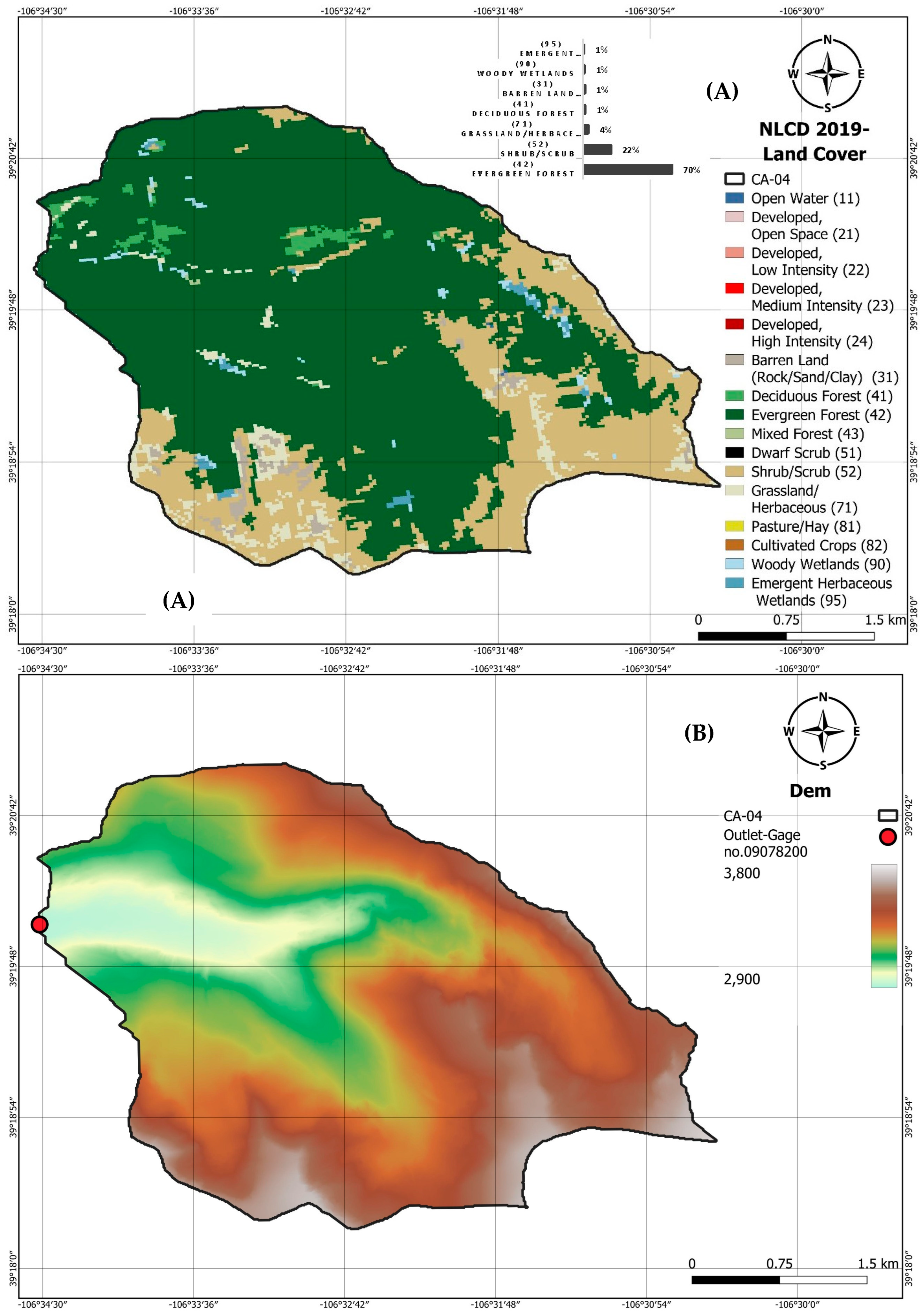
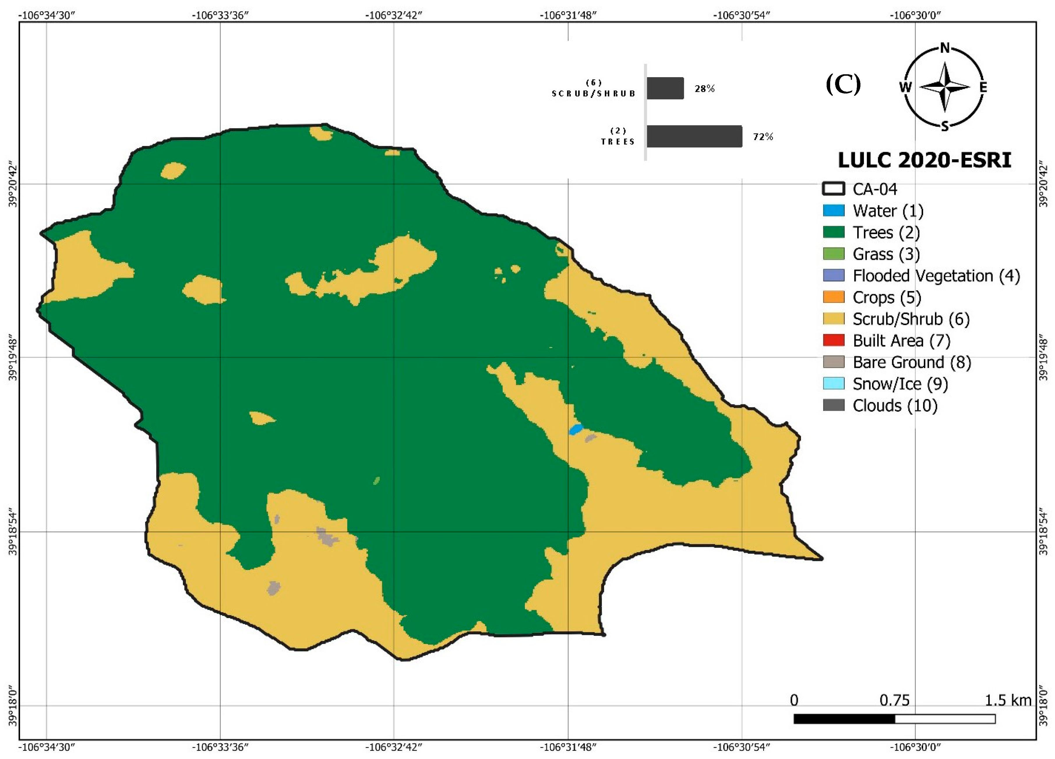
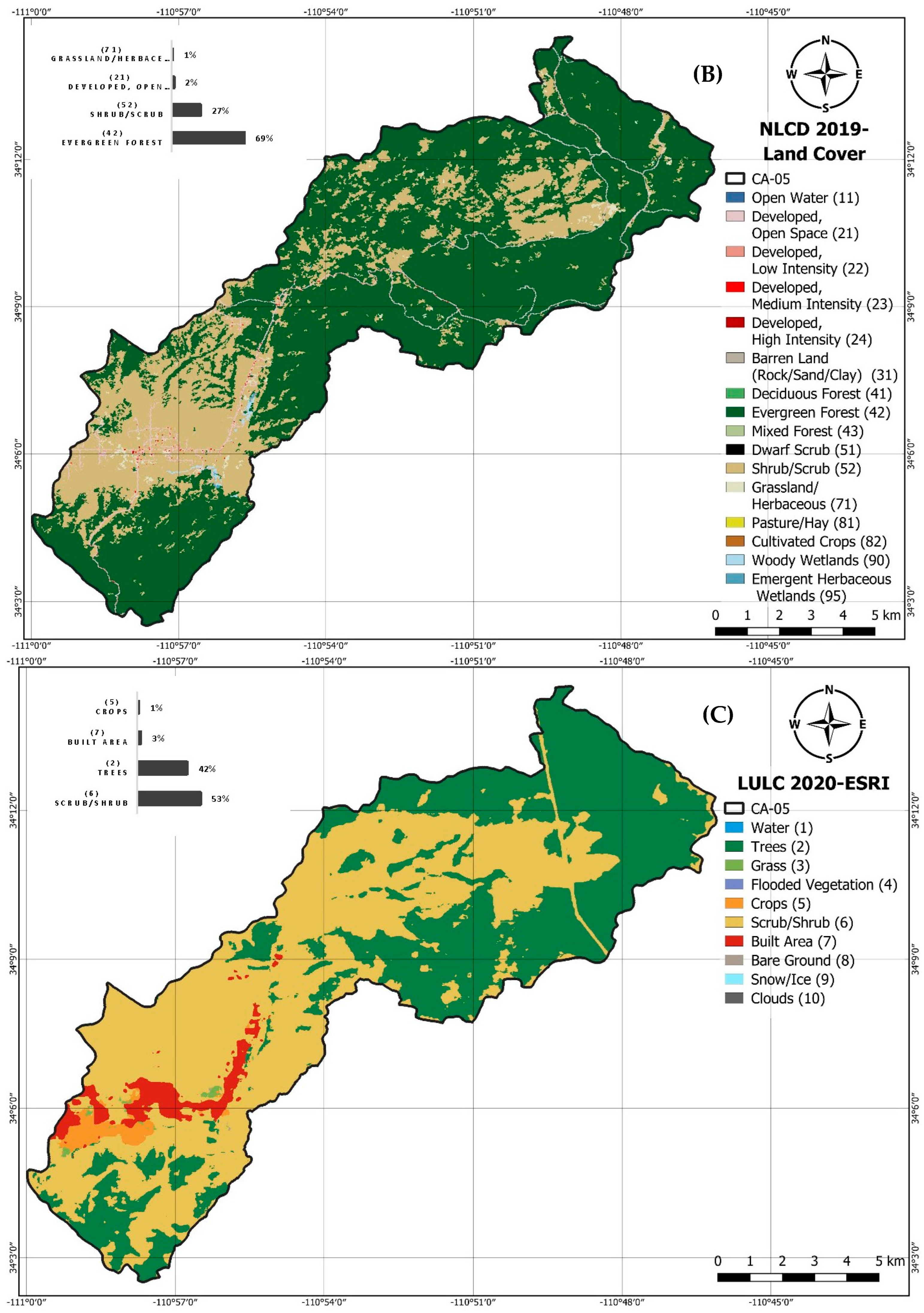
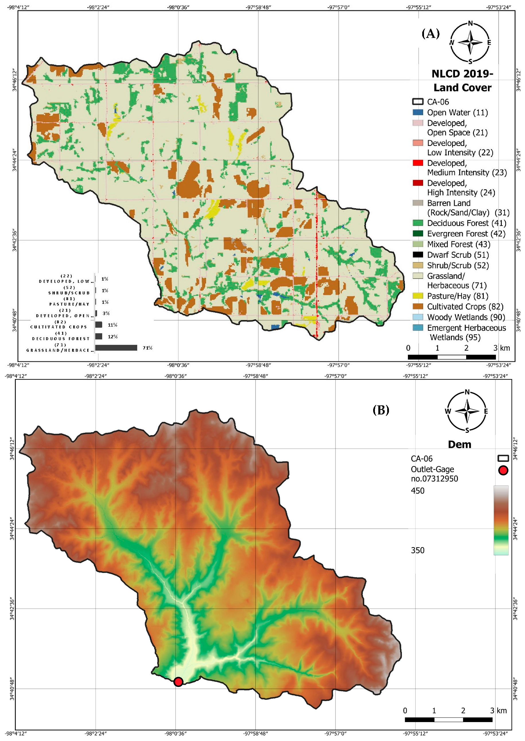
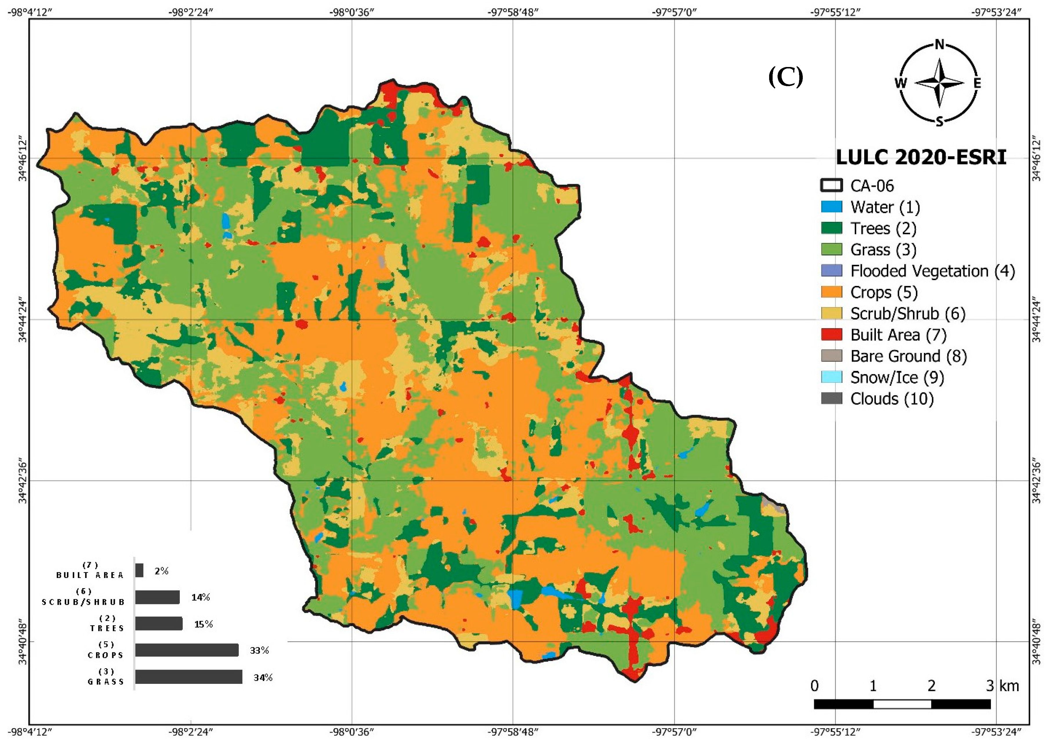
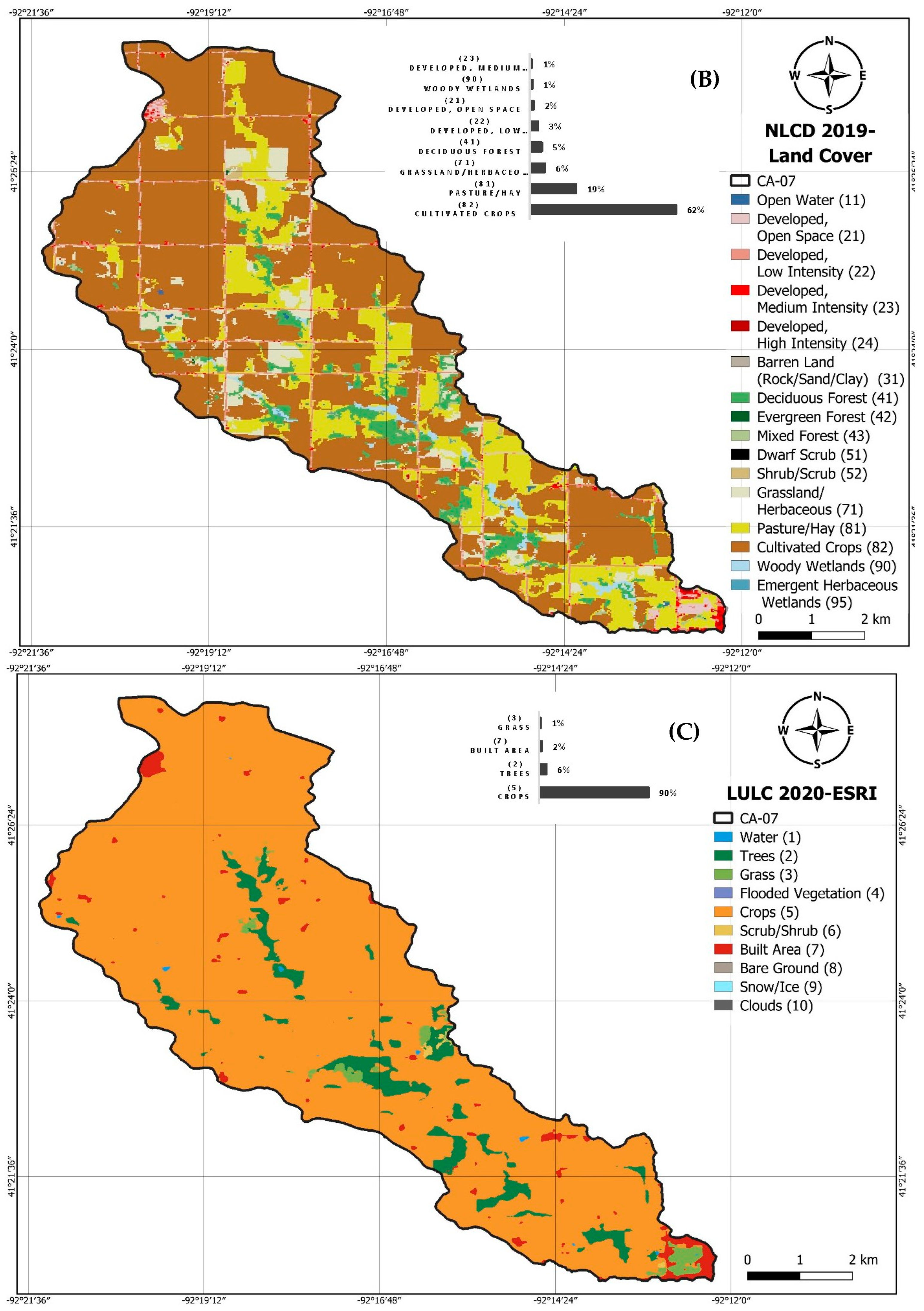
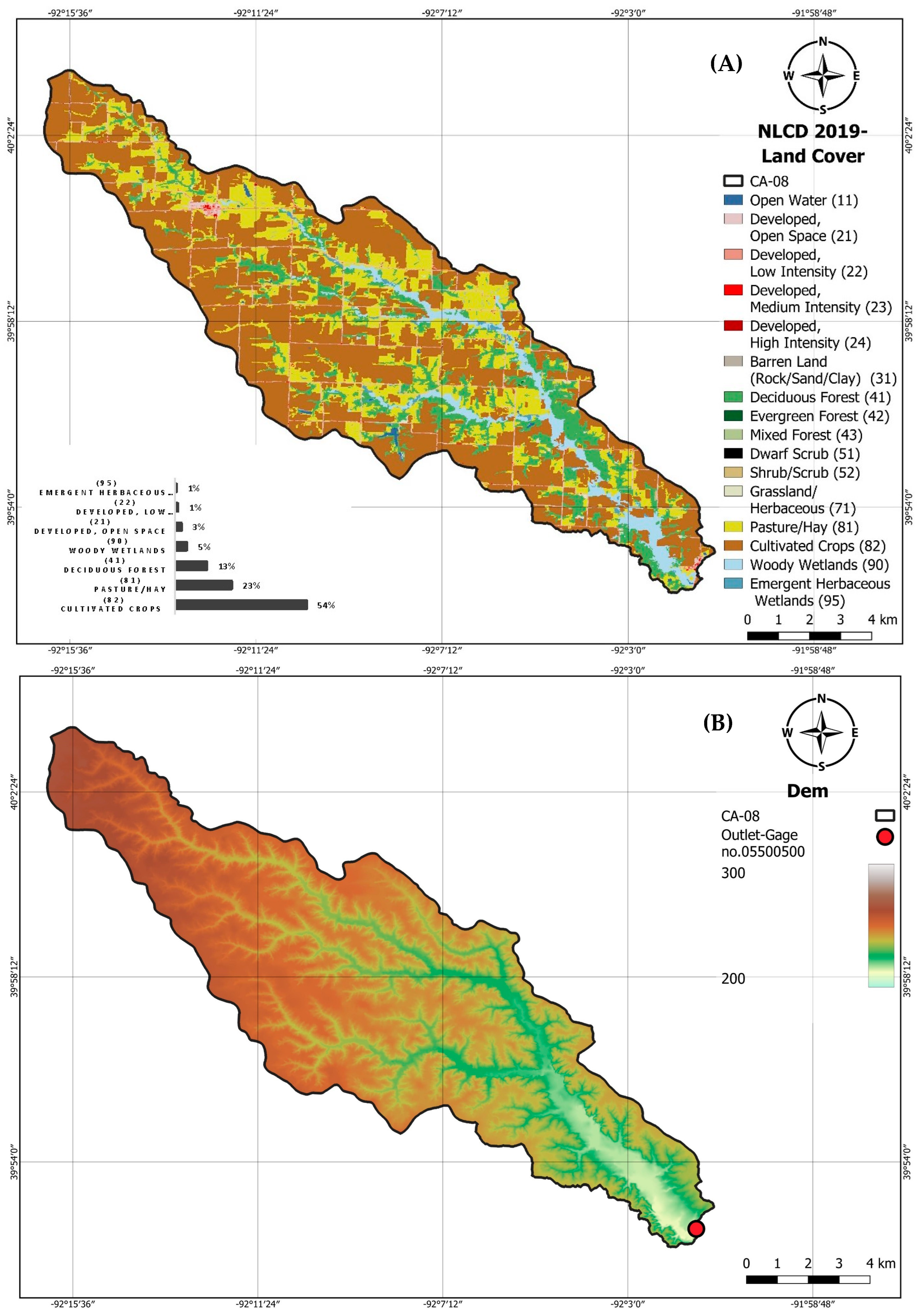
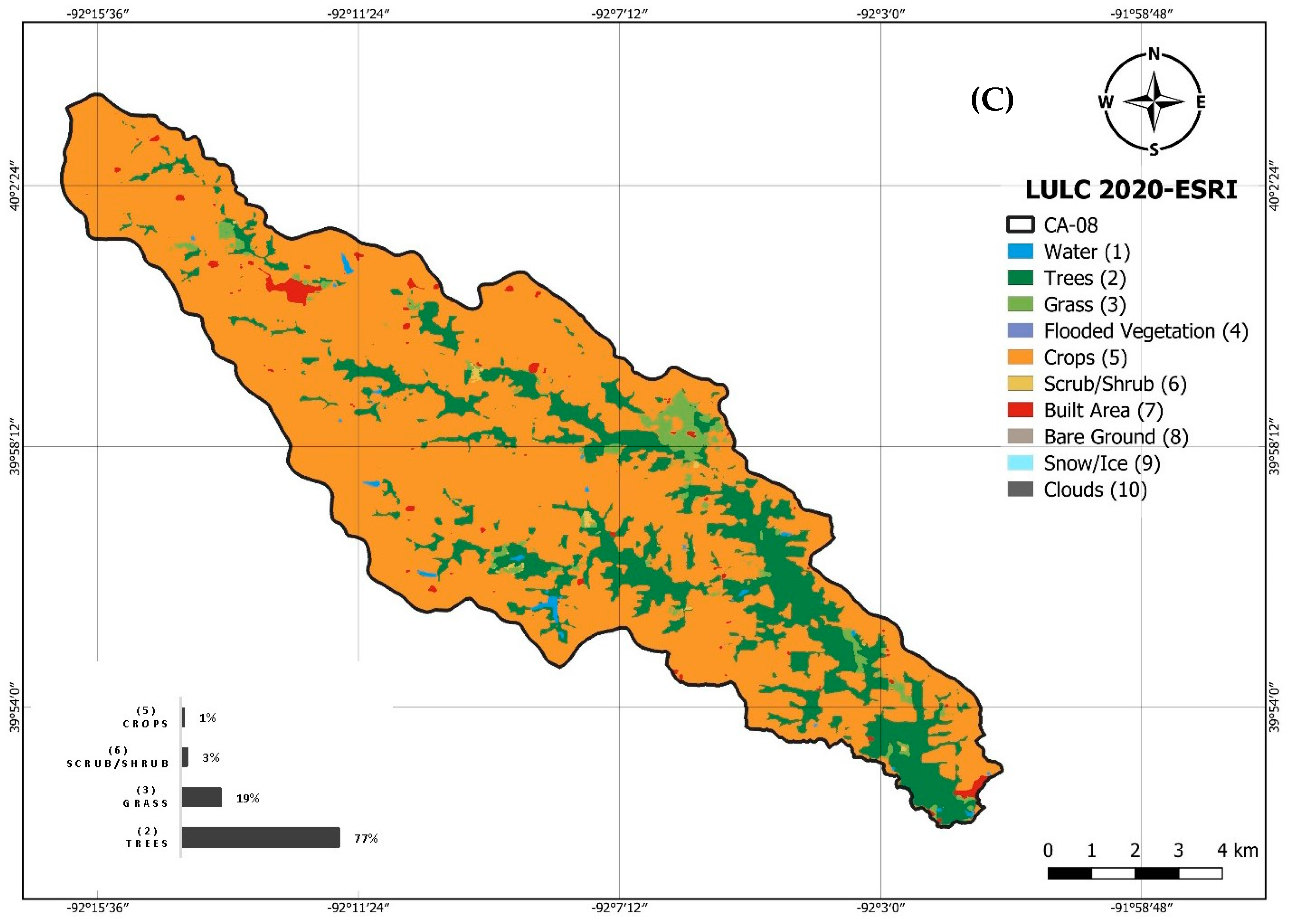
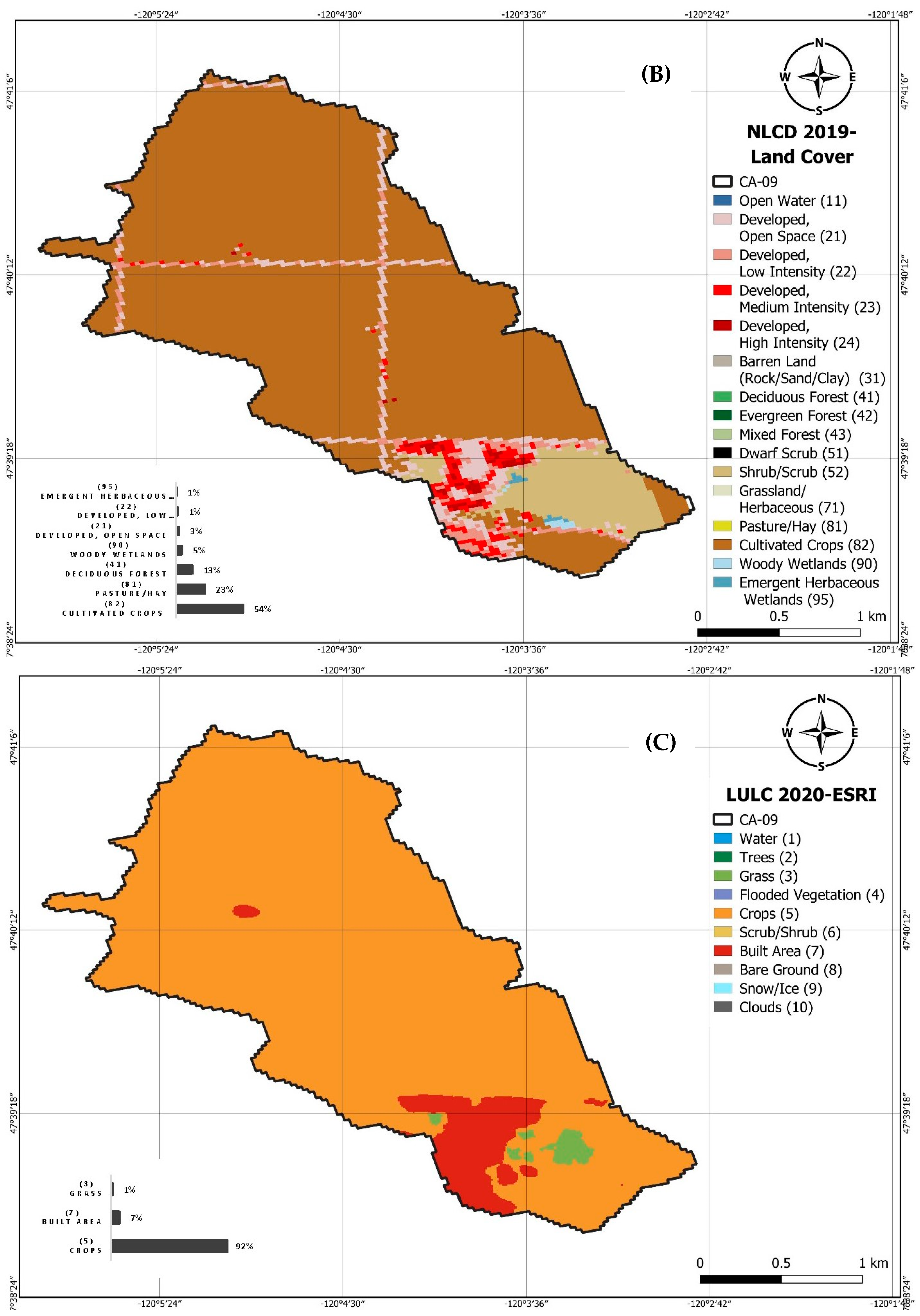
A confusion matrix was prepared in order to compare between the two datasets (NLCD 2019 and LULC 2020-ESRI), and cross-correspondence between both maps was achieved based on the full description for each class in the two datasets illustrated in
Table 2 and
Table 3. Based on the results shown in
Table 4, the “water” class was the most accurately mapped class (93%), followed by “trees” (86%), “crops” (81%), “built area” (77%), and “Grass” (71%). Lowest accuracy was obtained for the classes “Bare Ground” (57%), “Scrub/shrub lands” (56%), and “Flooded vegetation” (54%). The comparison results show an overall accuracy of around 72% with an error of 28% for the LULC 2020-ESRI map compared to the NLCD 2019 land-use map as a reference map (
Table 4). From the recent publications regarding the global-coverage maps’ accuracy assessment referenced to ground truth with a mapping unit of 250 m
2 data [
35], it was found that the overall accuracy of LULC 2020-ESRI maps had the highest value of 75%, which is consistent with the results from the current study.
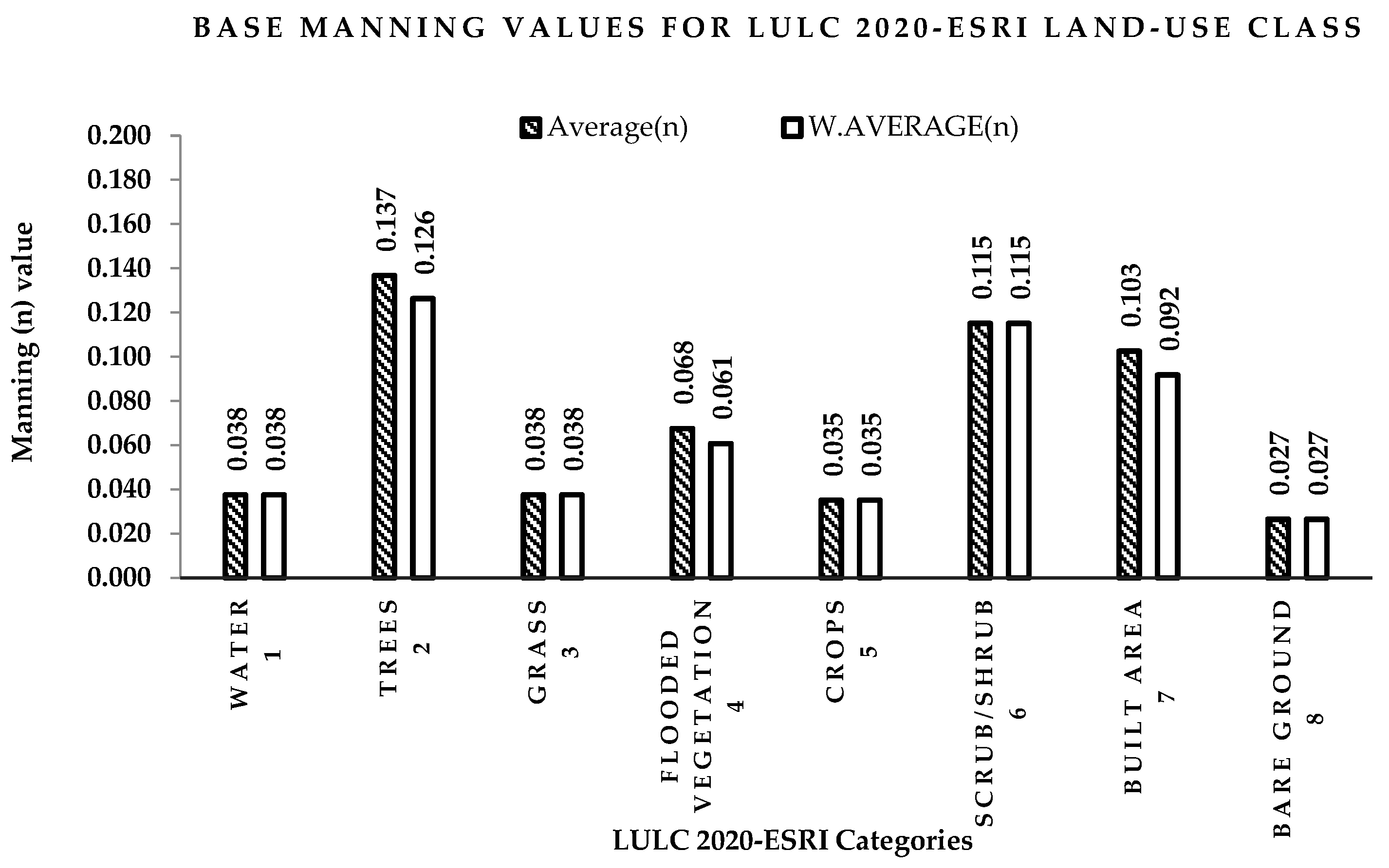
Table 5 illustrates the most matching classes between the two datasets; most of the classes in LULC 2020-ESRI were matched with only one class in the NLCD 2019 dataset, except for only three biased classes: grass, trees, and built area. Two statistical techniques, average and weighted average methods, were used to detect the proposed Manning’s roughness values for biased classes.
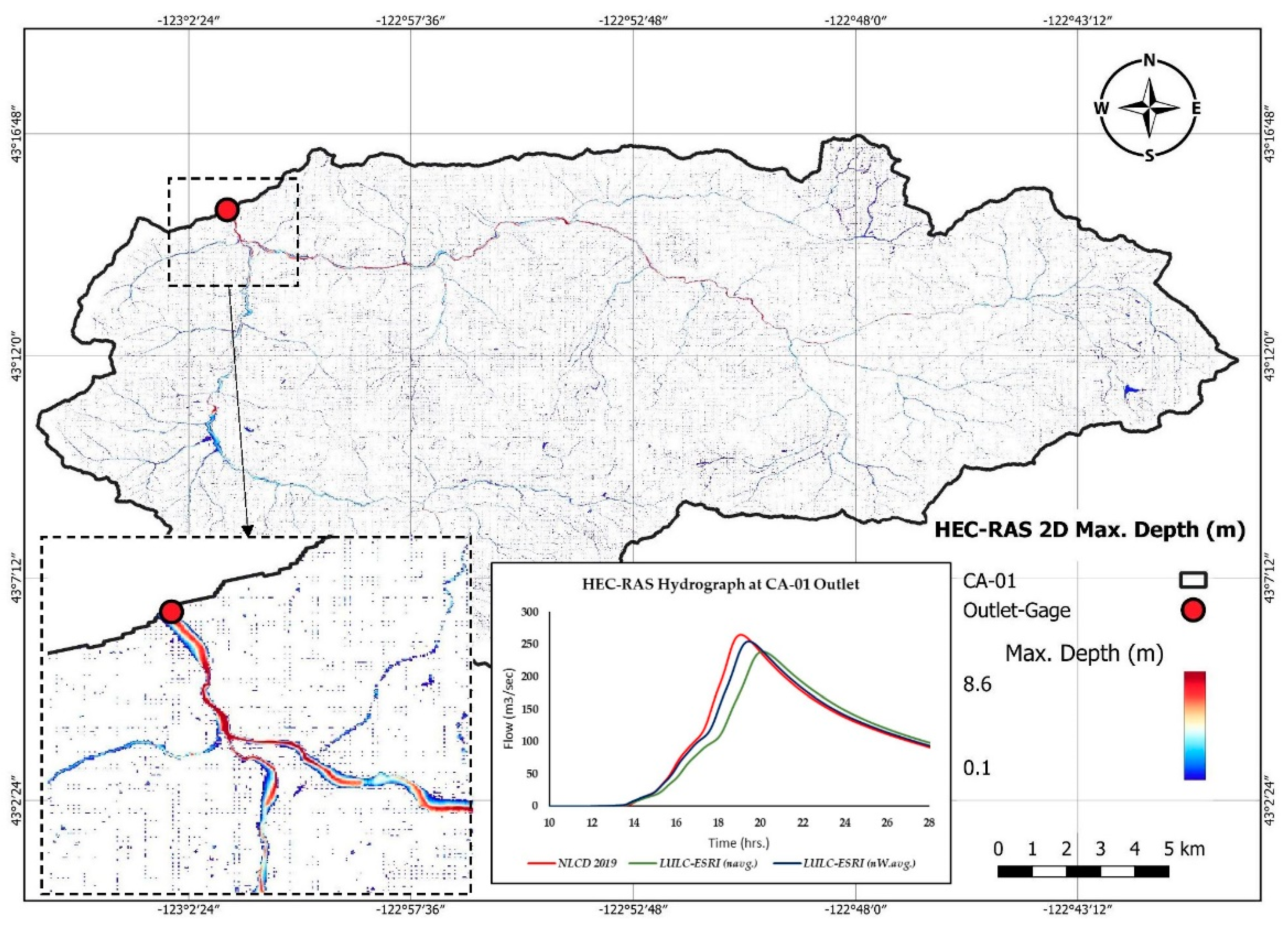
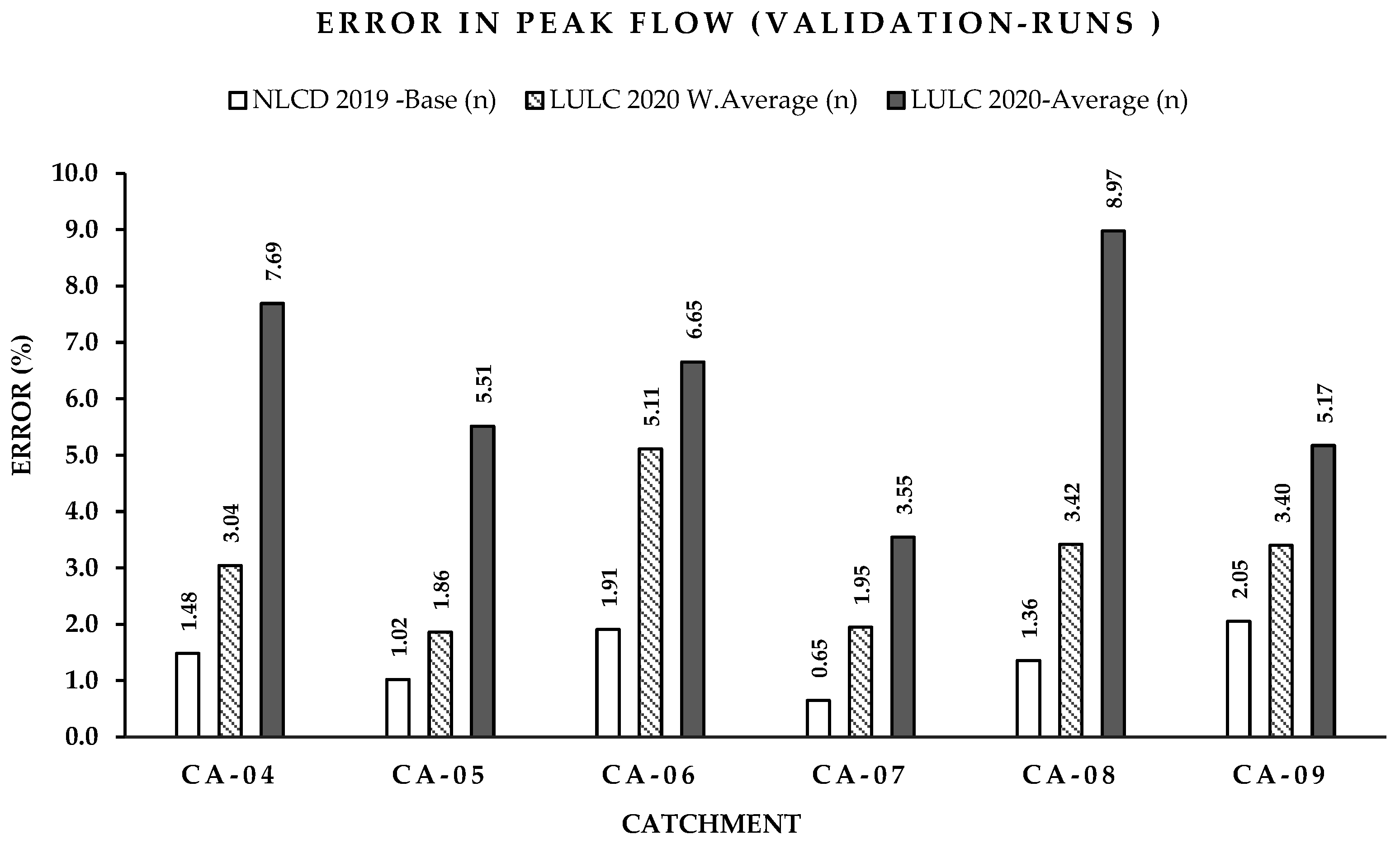
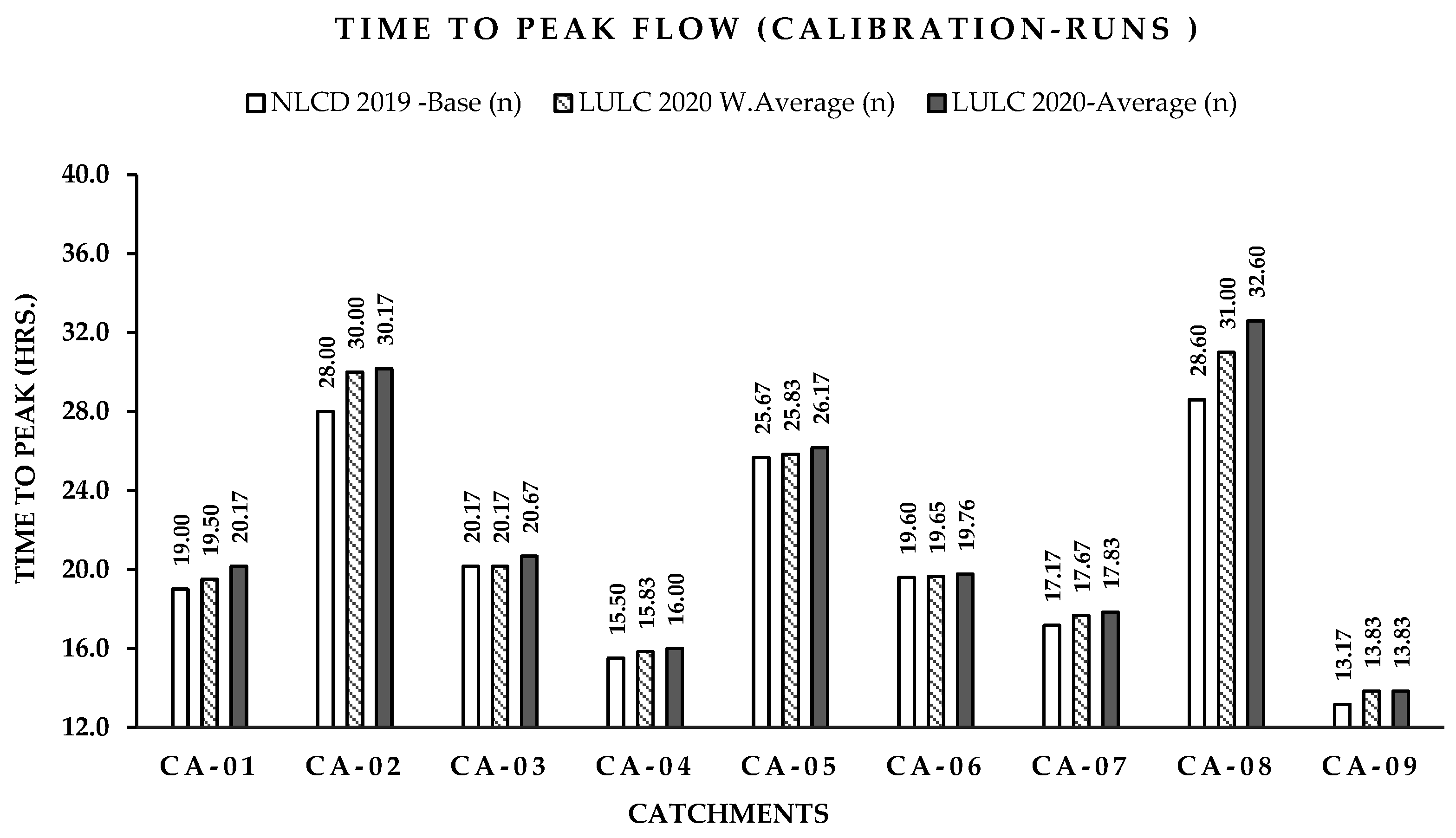
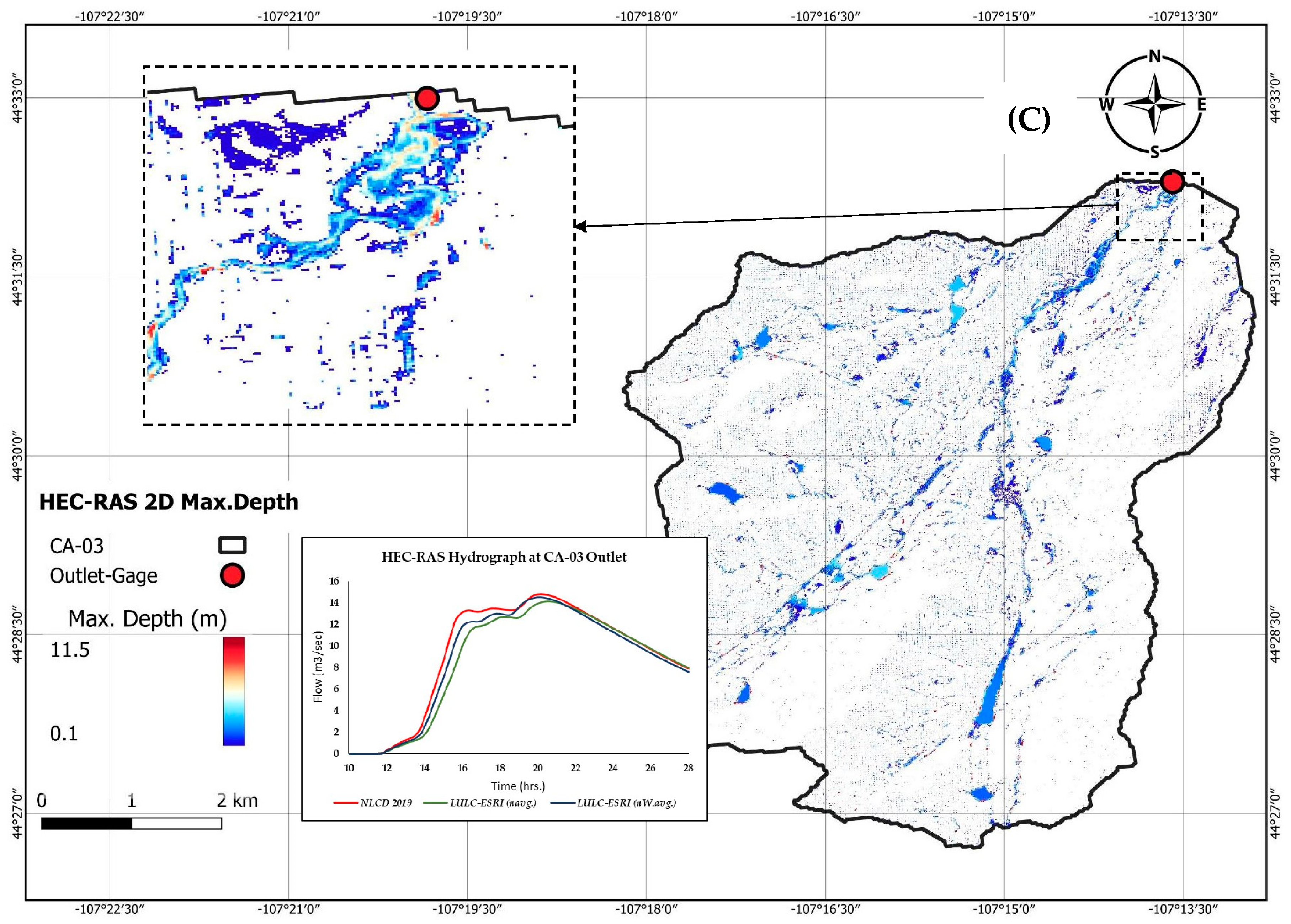
Based on the HEC-RAS 2D ROG analysis, implementing the proposed LULC 2020ESRI Manning’s roughness values for both average and weighted average methods (
Table 8), it was concluded that the weighted average values (
nw.avg) in all simulations showed relatively less time to peak and accurate peak-flow values. The average error in the peak flow is 5.22% (2.0% min. to 8.8% max.) for weighted average values (
nw.avg) compared to 8.5% (4.4% min. to 12.4% max.) when using the LULC 2020-ESRI map with average Manning’s roughness values (
navg) (
Table 8).
Appendix B shows flow hydrographs at the catchments’ outlets using the implemented maps.
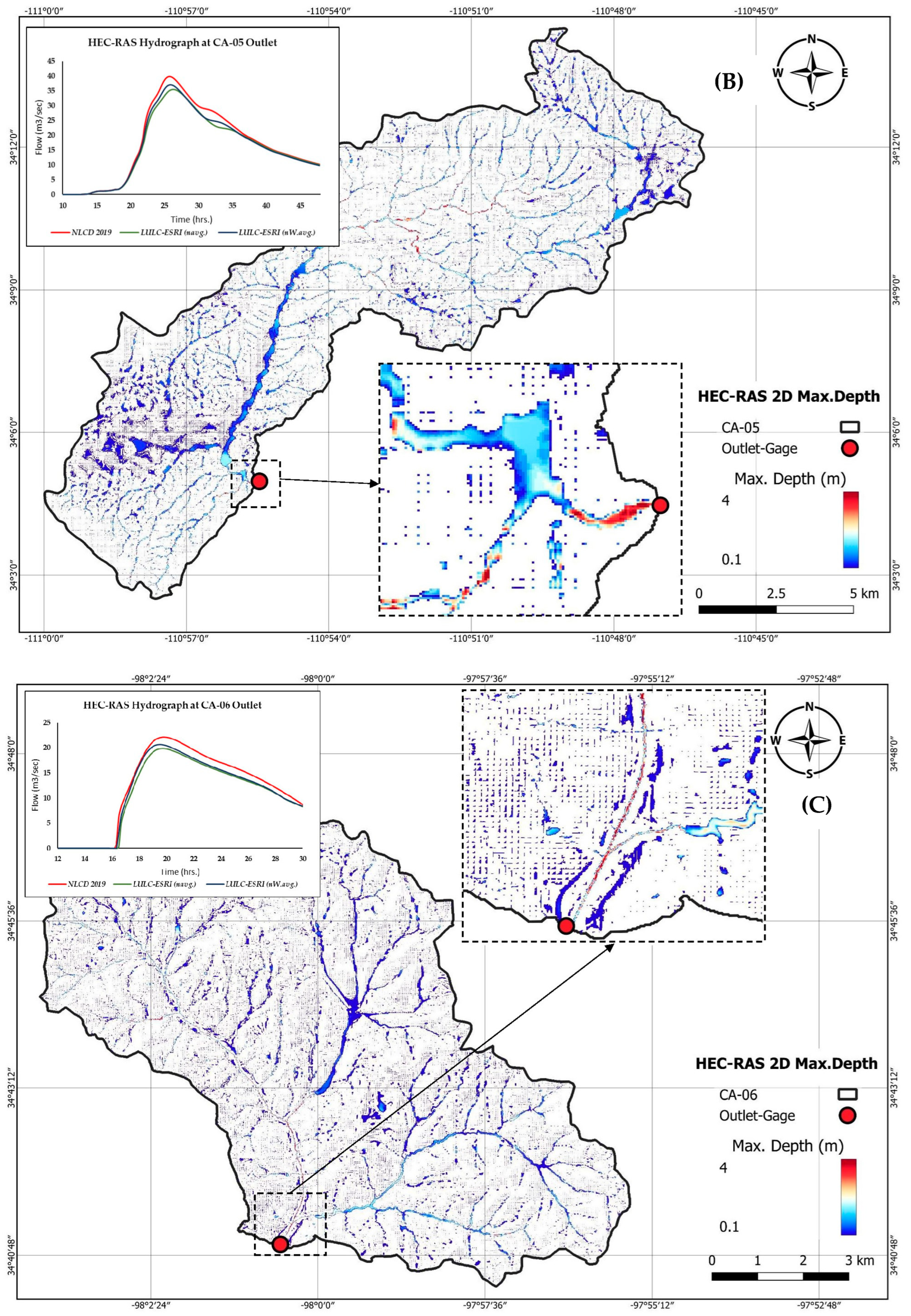
Using both of the statistical performance measures mean square error (RMSE) and mean absolute error (MAE), the HEC-RAS computational results were extracted and GIS tools were used to calculate floodplain inundated maximum depths and velocities. It has been concluded from the results in
Table 8 that the LULC 2020-ESRI maps using weighted average Manning’s roughness values (
nw.avg) in all simulations give lower error values with an overall value (RMSE
depth) of 2.7 cm, compared to 3.72 cm when using average Manning’s roughness (n) values, and an MAE
depth of 5.32 cm, compared to 7.75 cm when using average Manning’s roughness values (
navg). The same analysis was repeated to measure the errors (RMSE and MAE) in the velocity simulation, and it was found to confirm the same performance.
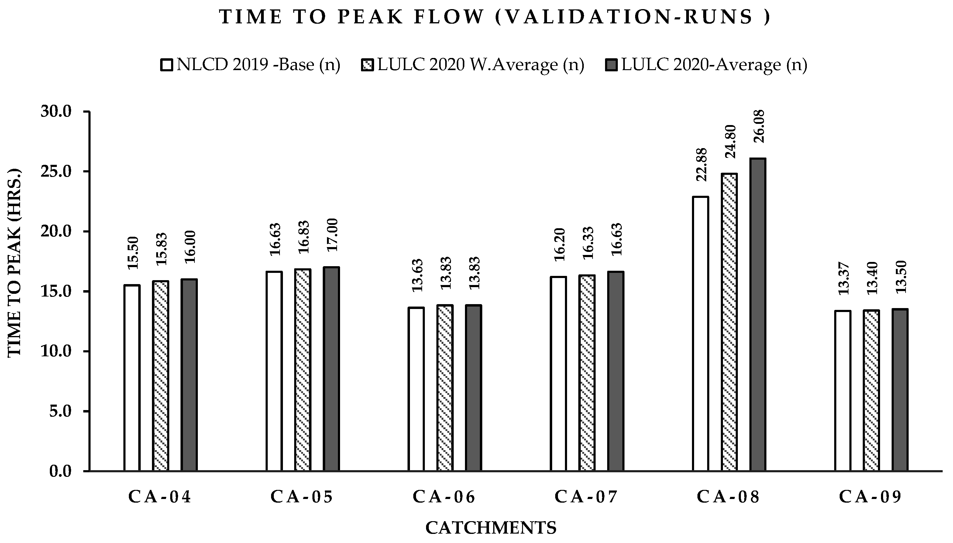
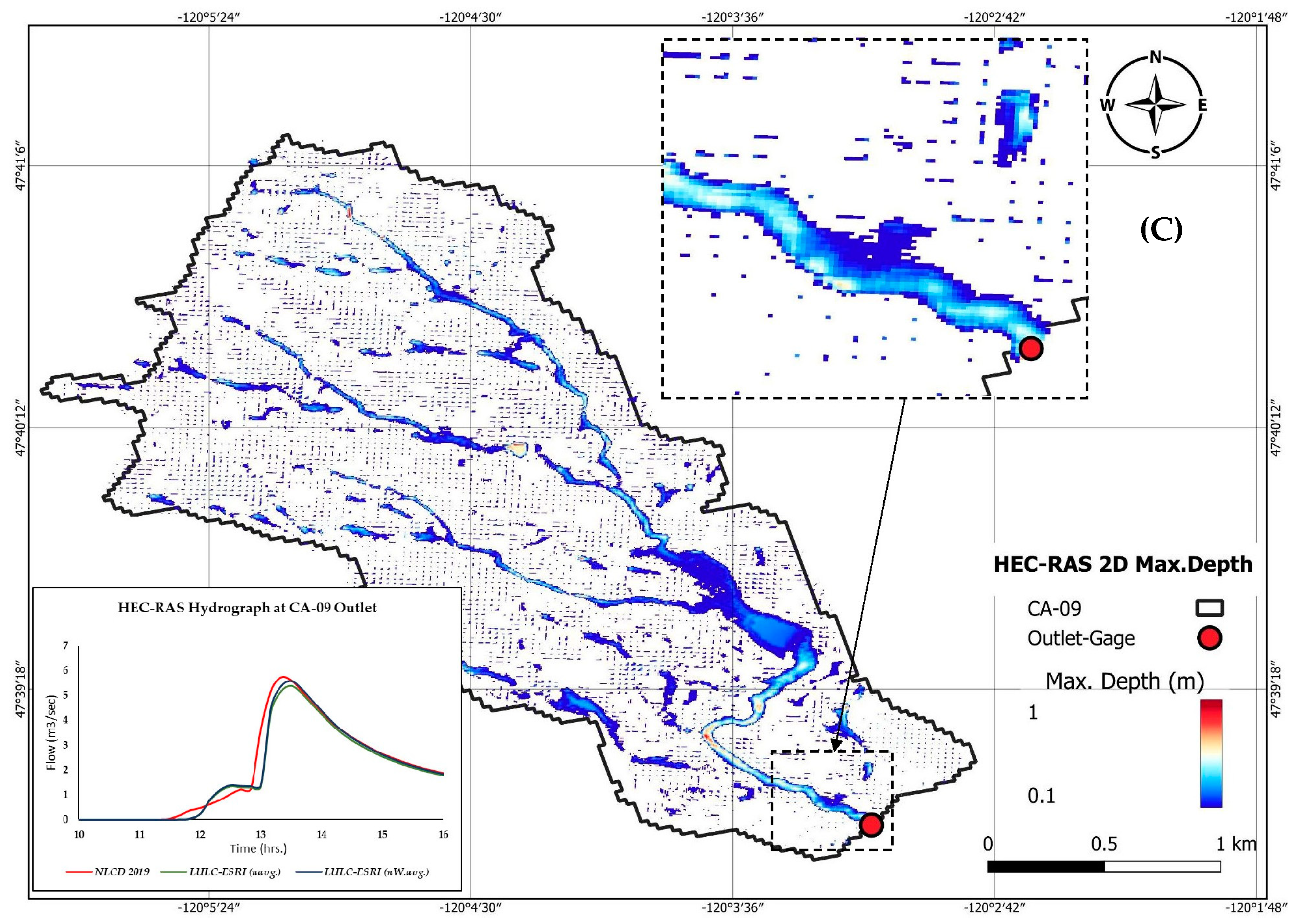
Testing the same catchments’ responses to the ROG HEC-RAS model using the validation dataset with 100-year 24 h rainfall (
Table 9) reveals that during high return periods, the error in capturing the peak value was reduced to an average of 3.13% when using weighted average Manning’s roughness values (
nw.avg), compared to 6.62% when using average Manning’s roughness values (
navg). Also, during the validation process, the error values in the water depth RMSE and MAE were with an average value of 3.8 cm and 4.2 cm, respectively, when using weighted average Manning’s roughness values (
nw.avg), compared to 4.7 cm and 8.1 cm, respectively, when using average Manning’s roughness values (
navg). The same analysis was repeated to measure the errors (RMSE and MAE) in the velocity simulation, and it was found to confirm the same performance.
One of the main outputs of the current study is the generated new base/reference for Manning’s roughness values for each class in the global land-use maps LULC 2020-ESRI. The generated maps using these Manning’s roughness values have been tested and confirmed to drive a low magnitude of error with an acceptable accuracy in both calibration and validation processes. Recommended Manning’s roughness values to be compatible with the global LULC 2020-ESRI maps are presented in
Table 10.


