Smooth Spatial Modeling of Extreme Mediterranean Precipitation

Abstract

Extreme precipitation events can lead to disastrous floods, which are the most significant natural hazards in the Mediterranean regions. Therefore, a proper characterization of these events is crucial. Extreme events defined as annual maxima can be modeled with the generalized extreme value (GEV) distribution. Owing to spatial heterogeneity, the distribution of extremes is non-stationary in space. To take non-stationarity into account, the parameters of the GEV distribution can be viewed as functions of covariates that convey spatial information. Such functions may be implemented as a generalized linear model (GLM) or with a more flexible non-parametric non-linear model such as an artificial neural network (ANN). In this work, we evaluate several statistical models that combine the GEV distribution with a GLM or with an ANN for a spatial interpolation of the GEV parameters. Key issues are the proper selection of the complexity level of the ANN (i.e., the number of hidden units) and the proper selection of spatial covariates. Three sites are included in our study: a region in the French Mediterranean, the Cap Bon area in northeast Tunisia, and the Merguellil catchment in central Tunisia. The comparative analysis aim at assessing the genericity of state-of-the-art approaches to interpolate the distribution of extreme precipitation events.

1. Introduction

The increasing hazard triggered by extreme precipitation events heightens the need to develop risk estimation approaches. The last decades have seen several deadly floods caused by extreme rainfall, particularly in the Mediterranean region (e.g., [1,2]). For example, during a heavy flood event in northeastern Tunisia in 2018, precipitation of around 200 mm occurred on a regional scale, producing a record of 297 mm in the Beni Khalled station in just a few hours [3]. The south of France was affected by a similar event in 2014 that left the city underwater with a record equivalent to more than six months of precipitation [4]. Every autumn, regions around the Mediterranean are affected by floods. The consequences of these phenomena are sometimes dramatic, including human and material losses, pollution of water resources and destruction of agricultural farms. Therefore, an effective forecasting system is essential to reduce the impacts of these disasters and to make the right decisions regarding flood risk assessment.

Extreme value theory (EVT) provides a proper parametric framework to model the distribution of extremes, particularly in hydrology [5]. The distribution of maxima over blocks of observations, often chosen to correspond to a time period of length one year, can be approximated by the generalized extreme value (GEV) family of distributions [6]. To convey information on the probability of extreme events, quantiles of the GEV distribution function are of particular interest because of their interpretation as return levels. This value is defined as the level of rainfall intensity that is expected to be exceeded on average once in a given year.

A major challenge in investigating the distribution of extreme rainfall events is to define a spatial representation at ungauged sites. Rainfall data are usually recorded from networks of rainfall stations in the study area. The spatial interpolation process involves using point data to find estimates at surrounding locations for which observations are not available. Several interpolation schemes have been proposed in the literature [7,8,9,10,11]. In classical initial interpolation approaches, the distribution parameters are estimated locally and then interpolated to obtain return level maps. For instance, in [12], local estimates of extreme rainfall intensities are interpolated to perform a regional analysis. Among others, the Inverse Distance Weighting (IDW) [13] and classical Kriging techniques [10,11], such as Ordinary Kriging [14], are frequently used. In this case, the grid estimate is obtained by the weighted average of the relevant observations, and each of the techniques uses a different weight calculation method.

More recent approaches, called “response surfaces”, consider that the distribution parameters vary according to geographical covariates. For instance, a smooth GEV fitting was proposed in [15] for mapping snow depth where parameters are directly modeled as function in space. In particular, the authors in [16] highlighted the use of several stations in regional approaches, known as region-of-influence, to reduce variance. Response surfaces provide a more flexible alternative to the regional approach by allowing the parameters to vary more flexibly in space. The relationship between GEV parameters and spatial covariates can be described by a regression model. Artificial neural networks (ANNs) can offer greater accuracy in estimating climate variables due to their ability to recognize patterns in the data [17]. As universal approximators, ANNs can model non-linear relationships between a set of inputs without making assumptions regarding the nature of data [18]. Owing to their flexible structure, neural networks can be related to other regression methods, such as the generalized linear model (GLM). For example, the authors in [19] conducted a spatial regression model with a GLM for the estimation of the GEV parameters to model the univariate marginal distributions. In this work, spatial modeling is carried out using response surfaces.

In order to obtain a spatial mapping of the extreme distribution at ungauged locations, covariates must be known everywhere in the study area. The main way to incorporate non-stationarity into the modeling of extreme events is to assume that the distribution parameters are no longer constant but vary as a function of covariates [5]. Researchers have highlighted the need to incorporate climatic and hydrological-based variables as covariates [20]. For example, in [21], an evaluation of several climatic covariates has been presented (altitude, longitude, latitude, mean annual rainfall, mean number of daily rainfall and mean daily rainfall). In [22], the authors proposed a model with annual precipitation as a covariate that exhibits good performance. We can also refer to the use of the North Atlantic Oscillation and Mediterranean Index in [23], the frequency of southern-type circulation patterns and air temperature in [20] and the Southern Oscillation Index in [24]. Satellite-based rainfall data are increasingly used, since they provide spatially detailed information about rainfall distribution [25].

The main objective of this work is to propose a smooth spatial modeling framework based on GEV response surfaces to interpolate extreme Mediterranean precipitation hazard. In Section 2, we described the three selected Mediterranean study areas and the used data set. We presented two techniques for modeling the relationship between GEV parameters and spatial covariates (GLM and ANN) (see Section 3). The model selection strategy involved determining the complexity level (i.e., the number of parameters in the model) by satisfying a trade-off between bias and variance, and finding the optimal set of covariates using a cross-validation technique. In Section 4, we presented the pointwise and the smooth spatial GEV parameters estimation. An assessment of the goodness-of-fit of each spatial model is conducted by comparing the confidence bands of the return levels at test stations.

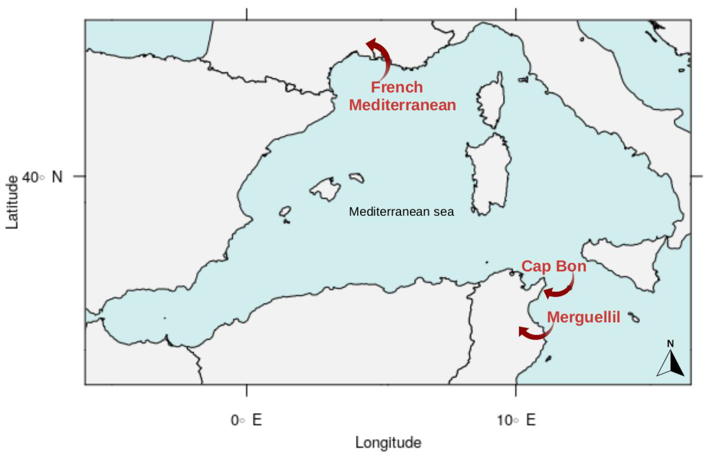
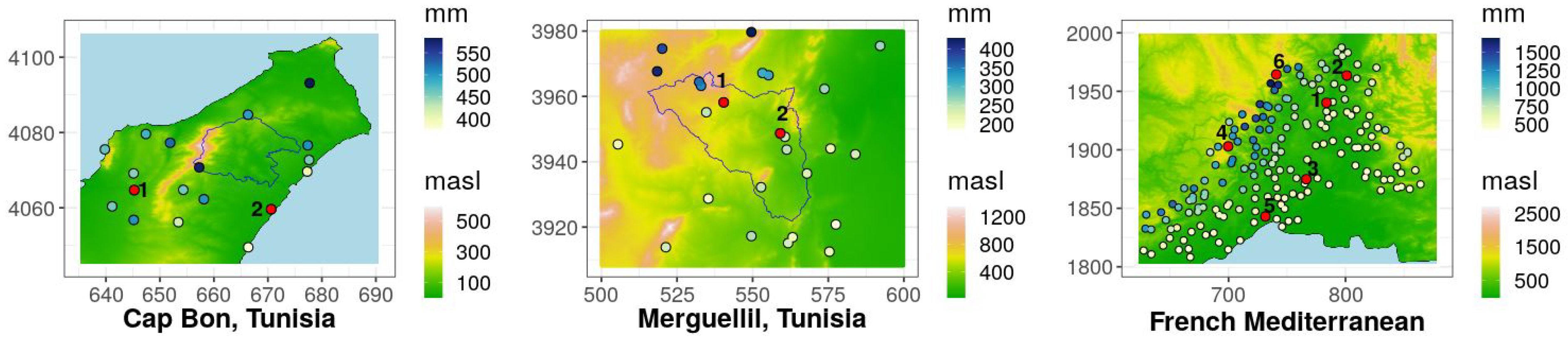
2. Study Area and Data

We consider three study areas marked by a Mediterranean climate: a region in the French Mediterranean, the Cap Bon area in northeast Tunisia, and the Merguellil catchment area in central Tunisia, which are located in Figure 1. These three Mediterranean regions are characterized by a north–south aridity gradient [26] and by a high spatial variability of precipitation with the occurrence of extreme events such as floods and droughts. The rainy season for the three study areas was fixed as the period from September to April (241 or 242 days per season). For each month of the year, the average rainfall totals show an increase between September and April and a decrease for the other months. For regions around the Mediterranean, other authors have considered the same rainy season (e.g., [10,27]). We note that all gauging stations in Figure 2 were selected by having at least 30 years of observations with less than 10% missing values per rainy season.

2.1. Rainfall Station Data

The French Mediterranean region is bounded on the south by the Mediterranean sea, on the west by the Cevennes mountain range (maximum elevation around 1687 m), and on the east by the Southern Alps (maximum elevation around 2694 m) (see the rightmost panel of Figure 2). Severe flooding, known as the “Cévenole”, occurs in this region, especially in the fall season [1]. From a climatic point of view, this study area is not homogeneous, since it contains two types of climate: the Mediterranean climate and the mountain climate [28]. Compared to the Mediterranean climate, the mountain climate is characterized by colder winters and milder summers. The hydrological processes are different due to the high variability of the rainfall regime, which means that the rainy season can be different. In order to work on a spatially homogeneous region and to define the same season for all study sites, we have chosen to classify the stations by climate type. We are only interested in the Mediterranean climate because of its high vulnerability to flooding. We selected stations by identifying sub-regions similar in terms of extreme rainfall behavior, inspired by the climatic regionalization approach presented in [29]. Each station was described by a vector containing 15 elements: the $95\%$ quantiles of the monthly maxima of daily precipitation for each of the 12 months of the year and the three corresponding geographical coordinates (longitude, latitude, altitude). Then, the K-means clustering method was applied to split the stations into two groups. Stations with a Mediterranean climate were retained. Those data were collected by Météo-France, with a spatial resolution of $0.4$ km, and they consist of daily precipitation records measured at 183 rainfall stations from 1958 to 2019. Average annual rainfall totals in this region over the rainy season vary from $433.4$ to $1697.3$ mm (see the rightmost panel of Figure 2). There are 20 stations with a complete number of observations and missing data for the remaining stations are up to $50.8\%$.

The region in central Tunisia, west of Kairouan, includes the Merguellil catchment, which covers an area of about 1200 km² upstream of El Haouareb dam [2,30] (see the central panel in Figure 2). Average annual rainfall totals over the rainy season vary from $185.6$ mm in the plain to $430.2$ mm in the highest part of the catchment. In this region, observations are available from 1900 to 2014 in 26 gauging stations, and the percentage of missing data varies between $40.35\%$ to $72.45\%$. We have also considered the Cap Bon region in northeastern Tunisia, which contains the Lebna catchment that covers an area of about 210 km² (see the leftmost panel of Figure 2). The maximum altitude is located in the mountainous region known as Djebel Abderrahmane and then decreases toward the coast. Daily precipitation data are available from 1919 to 2014 in 18 stations, with a percentage of missing data that varies between $19.29\%$ and $67.5\%$. Average annual rainfall totals over the rainy season range from $377.3$ to $583.2$ mm. Both daily rainfall data sets in Tunisia were collected from the Tunisian General Directorate of Water Resources.

2.2. CHIRPS Data Set

In addition to the covariates extracted from the geographical coordinates (longitude, latitude, altitude), we proposed to integrate the climatic variable obtained from the CHIRPS data set. Climate Hazards Group InfraRed Precipitation with Station data (CHIRPS) is a precipitation dataset developed by combining real-time observations with infrared data [31]. It is derived from three products: global climatologies, satellite estimates and gauge observations with daily, monthly and yearly temporal resolutions. From 1981 to the near present, CHIRPS data offer precipitation records with a spatial resolution ($0.05\times 0.05$ degree) and a quasi-global coverage 50° N to 50° S. This type of data will permit depicting the spatial pattern of precipitation in different regions. This information is not used directly to analyze extreme events because of its low spatial resolution and the existing bias between this data and local observations.

Daily CHIRPS GeoTIFF data were retrieved for the selected study area from https://climateserv.servirglobal.net/ (accessed on 17 November 2022). Average annual totals per rainy season (September to April) were computed from 1981 to 2019. The longitude and latitude coordinates were projected onto Lambert 2 coordinates. Bi-linear interpolation was applied to the averaged annual total values to match the DEM grid. The results of the interpolation are presented in Figure 3. For each gauged station, we assigned the value of the nearest grid cell in order to obtain the “chirps” covariate, which will be used as a spatial covariate.

2.3. Inter-Covariate Correlation Analysis

Kendall correlation coefficients between each pair of covariates were computed as a preliminary analysis to assess the amount of inter-dependence present in the covariates. Kendall’s coefficient varies from −1 and +1 and can be interpreted as follows: the closer it is to 1, the stronger the positive association is (variation in the same direction), and the closer it is to −1, the stronger the negative association. However, if the coefficient is close to zero, it means that there is no association. The correlation matrix for the three study regions is presented in Figure 4. For the French Mediterranean region, we observe a correlation coefficient that exceeds 0.5 for (x,y), (z,chirps), and (y,chirps); see the rightmost panel of the Figure 4. For Merguellil, see the central panel of Figure 4, where the covariate x has a negative correlation coefficient with all other covariates, especially a strong negative value with z-coordinate, which is obvious on the elevation map of the region (in Figure 2). For the Cap Bon region, see the leftmost panel of Figure 4: there is a moderate negative correlation coefficient for (x,chirps) and a lack of association for the other covariates.

3. Statistical Methods

3.1. Extreme Value Theory

As we are interested in extreme events, we need to focus on the behavior of the upper tail of the distribution. Extreme value theory (EVT) is a classical set of tools used to analyze extreme values [6]. We suppose that $X_1\dots X_n$ is a sequence of independent random variables and that $M_n=\max \{X_1\dots X_n\}$ is their maximum values. In this paper, the random variables are time series of daily rainfall observations from several gauged stations.

The fundamental theorem of [32] gives an asymptotic result allowing us to characterize the distribution of $M_n$. Suppose that there exists $c_n>0$ and $d_n\in \mathbb{R}$, two sequences of real numbers, such that:

$$\begin{array}{c}\hfill \underset{n\to \infty }{lim}P\left(\frac{M_n-d_n}{c_n}\le x\right)=G\left(x\right)\end{array}$$

(1)

where G is a non-degenerate distribution function that can be expressed as the generalized extreme value (GEV) distribution:

$$\begin{array}{c}\hfill G\left(z\right)=\exp -{\left[1+\xi \left(\frac{z-\mu }{\sigma }\right)\right]}_{+}^{-1/\xi }\end{array}$$

(2)

defined for the values of z for which $1+\xi (z-\mu )/\sigma >0$ and ($\mu$, $\sigma$, $\xi$) are the location, scale and shape parameters, respectively. The GEV distribution encompasses the three different behaviors of the maximum as controlled by the shape parameter. If $\xi >0$, the tail decays as a polynomial function; if $\xi =0$, the tail decays exponentially, and if $\xi <0$, the upper tail is bounded. The shape parameter is often assumed to be constant because it is difficult to estimate [6,33]. However, it would be advantageous to allow all GEV parameters to vary as a function of covariate [15,34].

The quantiles of the GEV distribution function are particularly significant because of their interpretation as return levels. The behavior of the extremes of the distribution function can be seen as the upper quantiles of a high order. To estimate these quantiles for the GEV, we invert Equation (2) such that $G\left(z_p\right)=1-p$ to obtain a return level $z_p$, with a return period $T=1/p$ which should be exceeded by the annual maximum with a probability p. The return level is given as follows:

$$z_p=\left\{\begin{array}{cc}\mu -\frac{\sigma }{\xi }[1-{(-log(1-p))}^{-\xi }]\hfill & \mathrm{if}\xi \ne 0\hfill \\ \mu -\sigma log(-log(1-p\left)\right)\hfill & \mathrm{if}\xi =0\hfill \end{array}\right.$$

(3)

The block maxima approach consists of sampling the observed maximum over a block, which is often chosen to correspond to a period of one year. In this paper, the block is considered as the rainy season in order to reduce the effect of temporal non-stationarity.

Several approaches have been proposed to estimate the parameters of the GEV distribution, including maximum likelihood (ML) or L-moments. The L-moment method estimates the set of parameters by matching the L-moments of the model to the L-moments of the empirical distribution [35,36]. It generally performs well with small samples and is usually more robust and less biased than the ML. However, applying the L-moment estimator is almost limited to stationary data. We will use the L-moment for the pointwise estimation and the ML for the spatial estimation.

3.2. Smooth Spatial Modeling for Extremes

3.2.1. Generalized Linear Models

The generalized linear model (GLM) is an extension of ordinary linear regression [37]. This model is widely used to model hydrometeorological variables [38,39]. The main idea of GLMs is to allow the linear model to be related to a response variable through a link function. These variables are no longer limited to the normal distribution, as assumed in linear regression, and they can come from any exponential family distribution (e.g., Gamma, Poisson). We consider that for a response variable Y assumed to follow the same exponential family distribution, and for $x_n$ a set of covariates, there exists the following relation:

$$g\left(E\left(Y\right|\mathit{x})\right)={\beta }_0+\sum _{i=1}^n{\beta }_i{x}_i.$$

(4)

The link function $g(·)$ is used to define a relationship between the linear predictor ${\beta }_0+{\sum }_{i=1}^n{\beta }_i{x}_i$ and the conditional mean of the distribution $E\left(Y\right|\mathit{x})$. The choice of this function depends on the nature of the response variable (e.g., identity, log). The set of parameters $\beta$ is estimated by the maximum likelihood [40].

Smooth spatial modeling can be achieved by considering that the input variables $\mathit{x}$ are covariates reflecting spatial information. Suppose that $g\left(z\right)=(g_1\left(z\right),g_2\left(z\right),g_3\left(z\right))$. The GLM applied to the GEV distribution can be written as follows:

$$g_1\left(\mu (Y,{\beta }_{\mu })\right)={\beta }_{{\mu }_0}+\sum _{i=1}^n{\beta }_{{\mu }_i}{x}_i$$

(5)

$$g_2\left(\sigma (Y,{\beta }_{\sigma })\right)={\beta }_{{\sigma }_0}+\sum _{i=1}^n{\beta }_{{\sigma }_i}{x}_i$$

(6)

$$g_3\left(\xi (Y,{\beta }_{\xi })\right)={\beta }_{{\xi }_0}+\sum _{i=1}^n{\beta }_{{\xi }_i}{x}_i,$$

(7)

where $g\left(z\right)=(z,\log (z),\log (z+0.5\left)\right)$. The link function for the scale parameter is the log function to ensure its positivity. For the shape parameter, it is assumed that $\xi >-0.5$ to ensure the regularity of the maximum likelihood estimators. The GLM is implemented by the VGAM package [41] for the R statistical computing environment.

3.2.2. Artificial Neural Networks

The artificial neural network (ANN) is a flexible model capable of identifying complex non-linear relationships between inputs and outputs [18], without predefined information about the underlying process involved. They are composed of a set of stacked and interconnected layers: the first layer contains inputs, the last layer contains outputs, and the layers in between are called hidden layers. In this work, we will use a feed-forward neural network with one hidden layer, i.e., the information flow is unidirectional from input to output. The neurons feed the neurons of the following layers to obtain final output data. Associating an ANN with the GEV distribution is equivalent to considering that the parameters $(\mu ,\sigma ,\xi )$ are the outputs of the network.

The first step of training the neural network (forward phase) is presented as follows. Suppose that $\mathit{x}=\{x_1,\dots x_n\}$ are the input variables (or covariates). Each neuron j of the hidden layer transforms m linear combination of inputs to give an output:

$$\begin{array}{c}\hfill z_j=h(\sum _{i=1}^n{w}_{ji}{x}_i+w_{j0}),\end{array}$$

(8)

with $j=1,\dots ,m$. $w_{ji}$ is the weight between two neurons i and j, and $w_{j0}$ is the bias of the neuron j. We took the hyperbolic tangent as the activation function $h(.)$ of the hidden layer. To obtain the outputs ${\theta }_k=(\mu ,\sigma ,\xi )$, we proceed to another linear combination with the activation function $f(.)$ over $z_j$:

$$\begin{array}{c}\hfill {\theta }_k=f(\sum _{j=1}^m{w}_{kj}{z}_j+w_{k0}).\end{array}$$

(9)

For $\mathit{y}=\{y_1,\dots ,y_n\}$ that comes from a GEV distribution, the conditional log likelihood is defined as a cost function to optimize the parameter values. To ensure that $-0.5<\xi <0.5$, we assumed that $\xi =\frac{2}{k}-0.5$ for all $k>2$. The cost function can be written as follows:

$$\begin{array}{cc}\hfill l(\theta ;y)& =\log \sigma +(1+\frac{1}{\xi })\sum _{i=1}^n\log \left[1+\xi \left(\frac{y_i-\mu }{\sigma }\right)\right]+\sum _{i=1}^n{\left[1+\xi \left(\frac{y_i-\mu }{\sigma }\right)\right]}^{-\frac{1}{\xi }}\hfill \\ \hfill & =\log \sigma +\left(\frac{2+0.5k}{2-0.5k}\right)\sum _{i=1}^n\log \left[1+\frac{(2-0.5k)(y_i-\mu )}{k\sigma }\right]+\sum _{i=1}^n{\left[1+\frac{(2-0.5k)(y_i-\mu )}{k\sigma }\right]}^{-\left(\frac{k}{2-0.5k}\right)}.\hfill \end{array}$$

(10)

The second step (the backward phase) consists of the computation of the gradient of the log-likelihood in Equation (10) with respect to all the weights of the network using the back-propagation algorithm, and the optimization is completed with a gradient descent algorithm. Weights are given randomly at the first step of the training and then updated until convergence.

The complexity level is controlled by the number of hidden units of the neural network. Indeed, the number of hidden units directly influences the number of weights in the ANN and hence its flexibility. The choice of the number of hidden units must satisfy the bias–variance trade-off: if it is too small, the ANN is biased (a phenomenon also called under-fitting), if it is too high, the ANN has a large variance (a phenomenon also called over-fitting). Therefore, the selected number of hidden units must simultaneously minimize the bias and variance of the ANN. One way to do this is to use cross-validation, which is a process that aims to estimate the generalization capability, i.e., the ability to perform well on unseen data.

In this work, to estimate the generalization capability, we will use the 10-fold cross-validation technique summarized in the following steps:

• Shuffle the data set randomly.
• Split the data set into k = 10 folds.
• For each fold:

  –

  Define that fold as the validation data set.

  –

  Define the remaining folds as the training data set.

  –

  Fit the model on the training set and evaluate on the validation set.

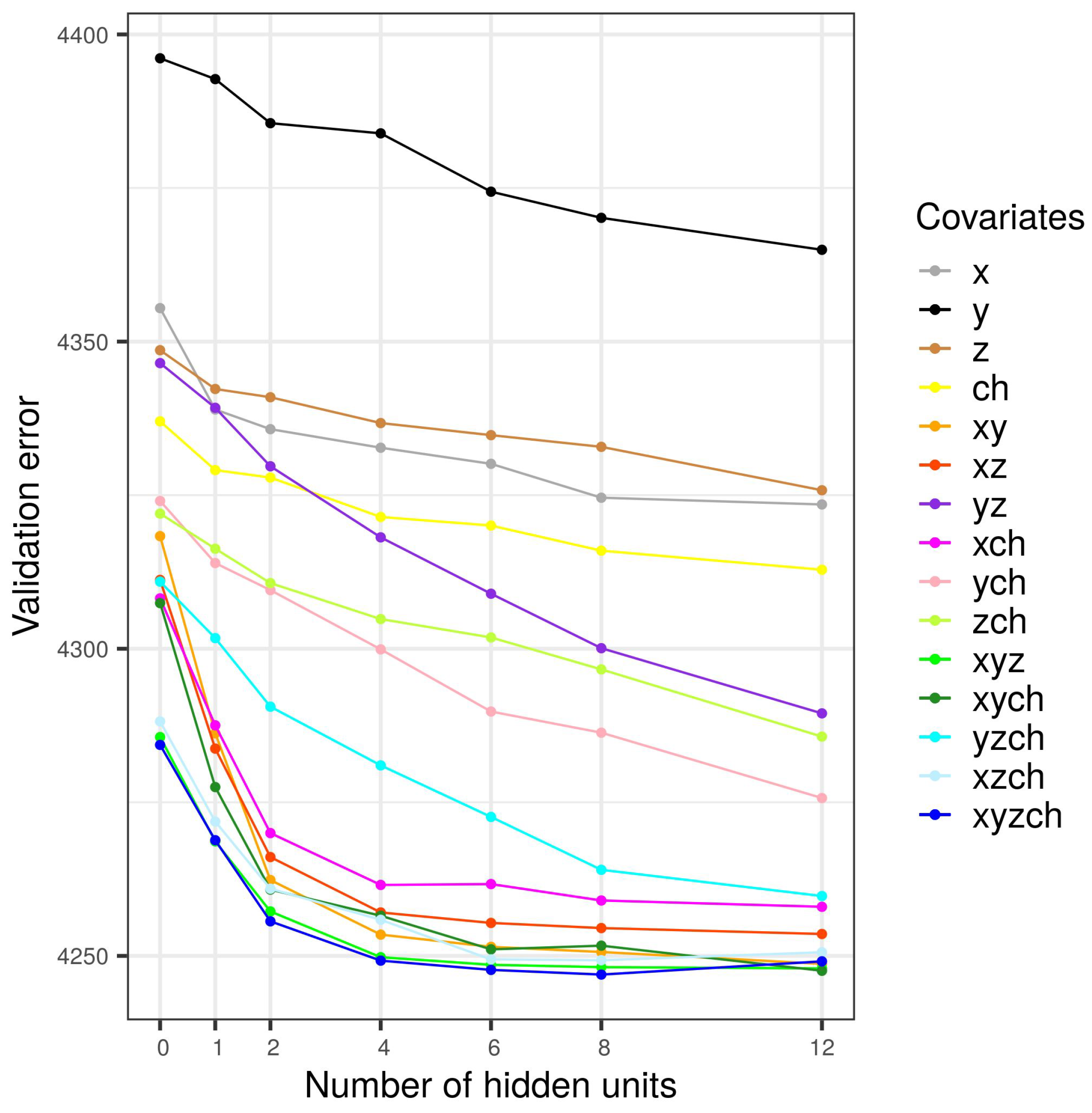
• The error is calculated as the average of the error over all validation sets. The optimal number of hidden units corresponds to the minimum of errors.

4. Results

The present research compares two spatial models (GLM and ANN), which are defined in Section 3, applied to the daily rainfall data sets described in Section 2. In Section 4.1, we explored the estimation of the GEV parameters locally (i.e., for each gauging station) to gain insight into the spatial estimation. Then, in Section 4.2, we proceeded to build the two spatial models by identifying the covariates and the appropriate level of complexity (i.e., the number of hidden units). Finally, comparison and evaluation were dedicated in Section 4.3.

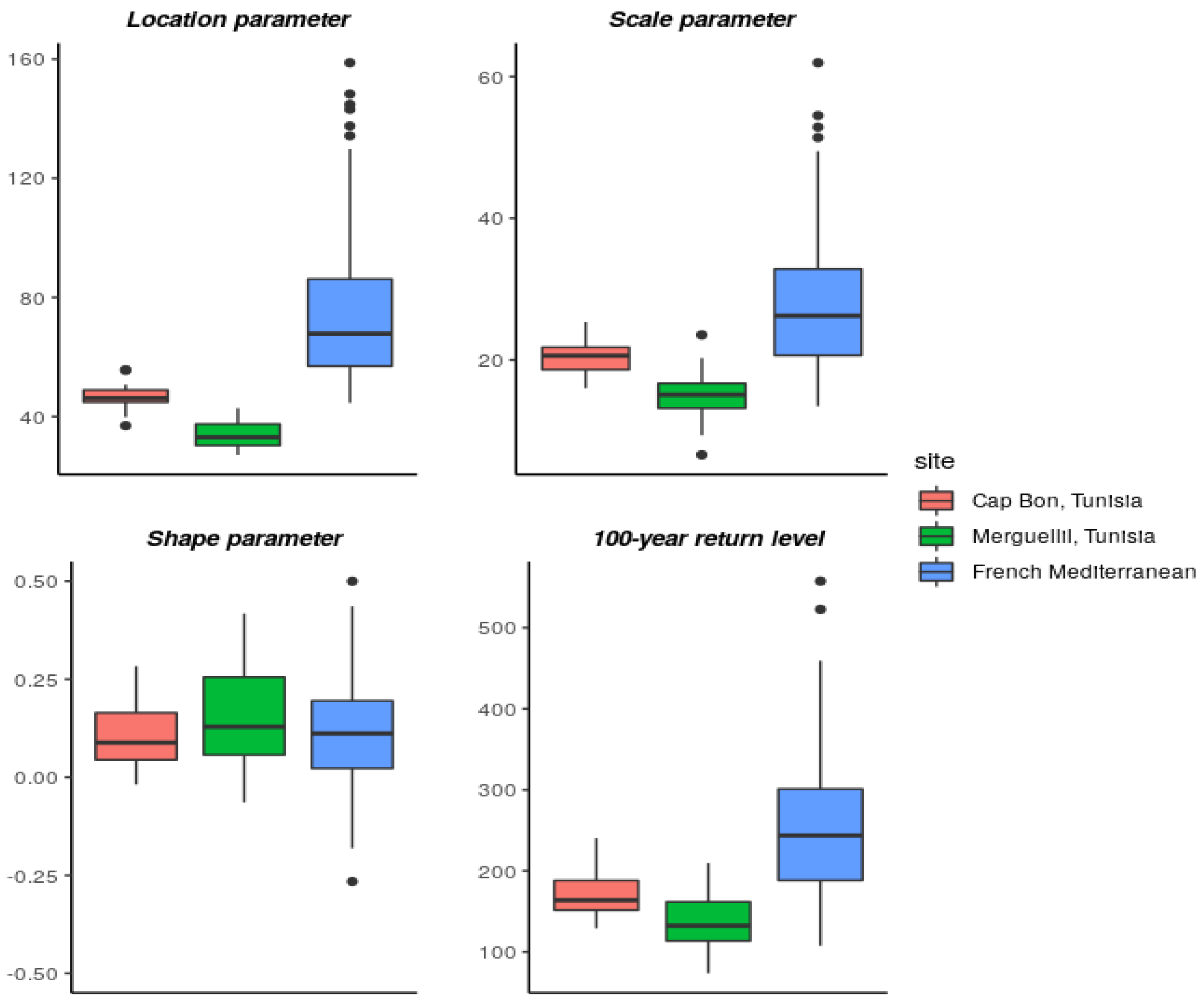
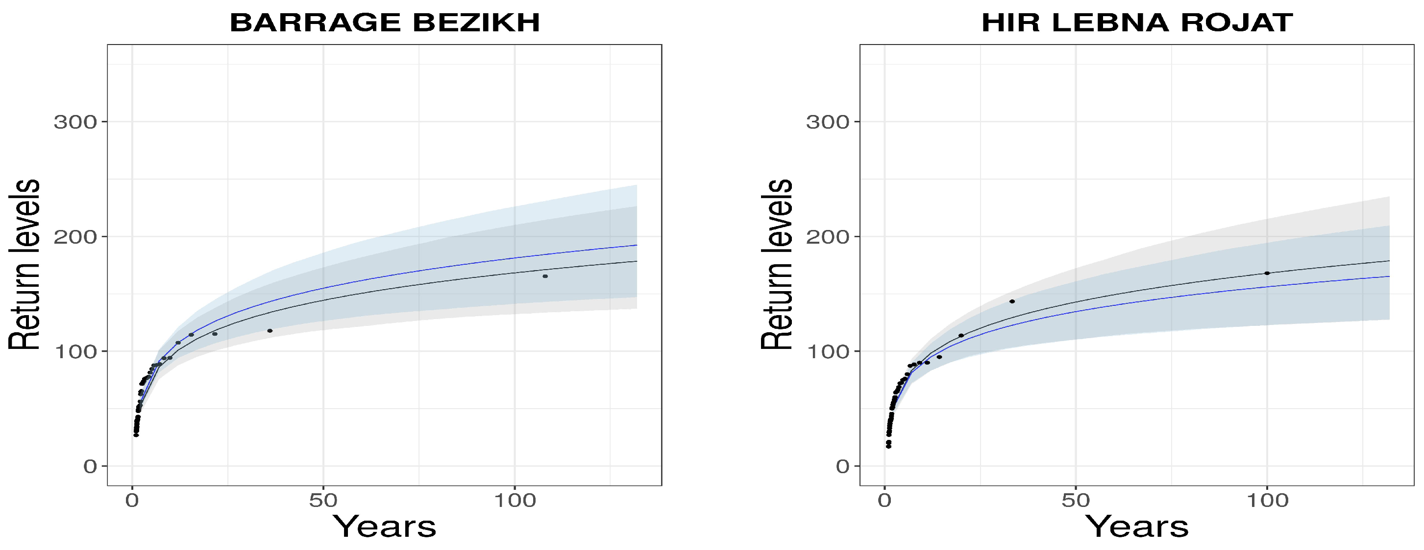
4.1. Pointwise GEV Parameters Estimation

Once the maxima per rainy season have been fixed for each station s, the GEV distribution parameters $({\mu }_s,{\sigma }_s,{\xi }_s)$ are estimated locally by the L-moments method. The 100-year return levels were computed from these estimates by Equation (3). A summary of all point estimates is presented in Figure 5. All shape parameter estimates are between −0.5 and 0.5. Indeed, the majority of stations have positive values of the shape parameter indicating the heaviness of the tail of the distribution (very large rainfall events can occur). However, fewer stations have negative values in the Merguellil and Cap Bon region compared to the French Mediterranean (32 stations).

Pointwise parameter estimates can only give information for the few stations where data are available. It will be more interesting to investigate the spatial variation of these parameters at any point in space. The following part of this article will focus on this issue.

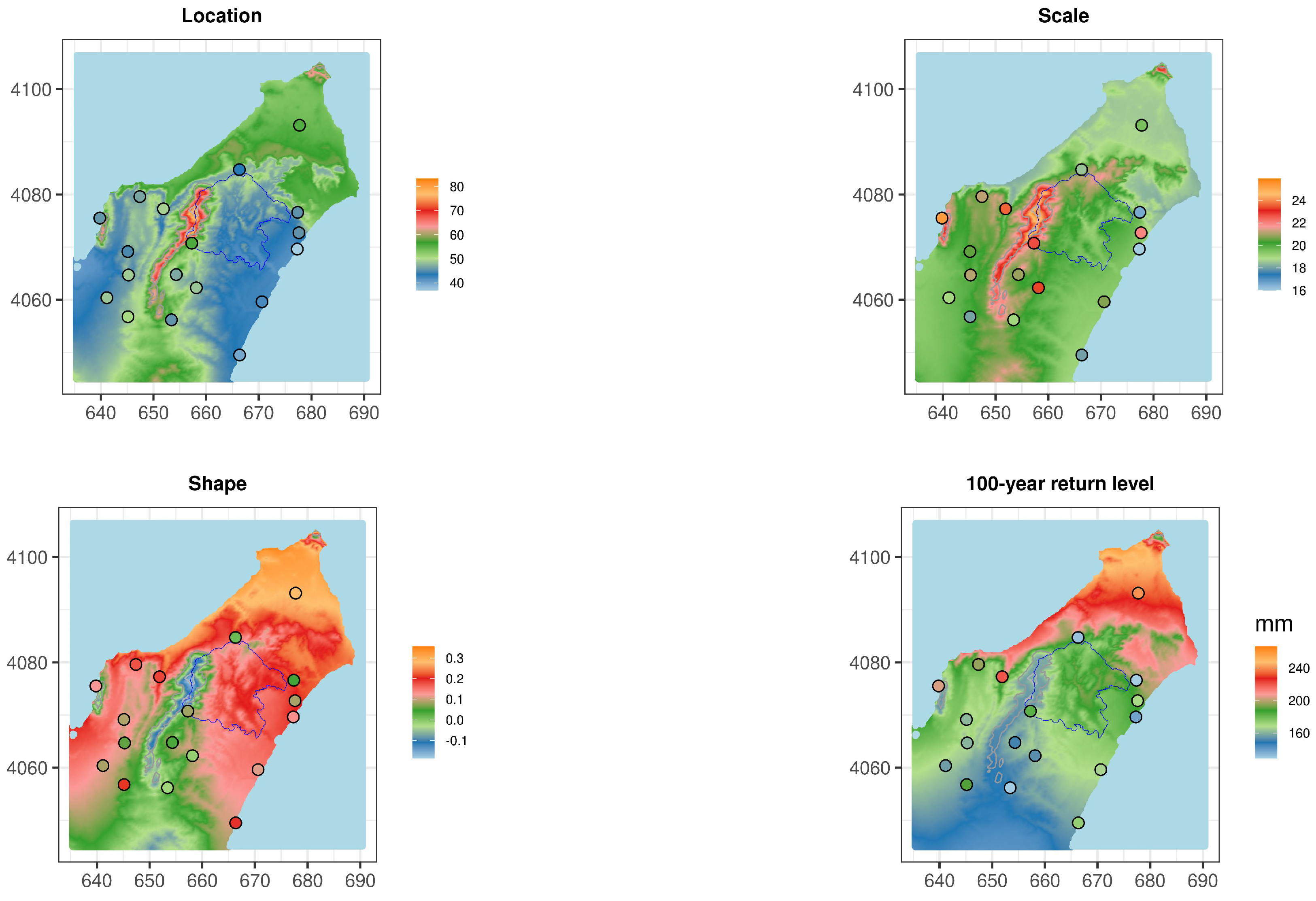
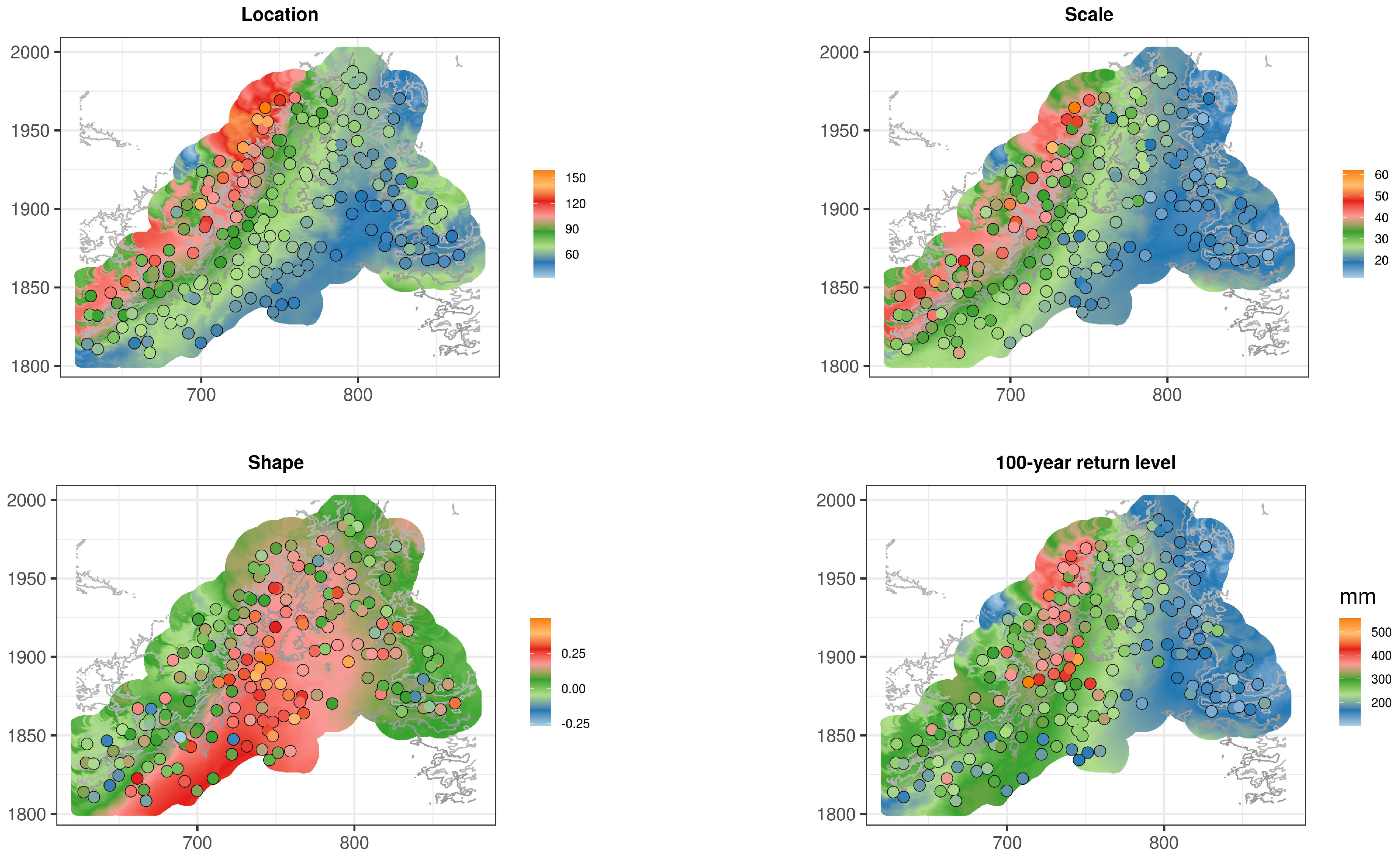
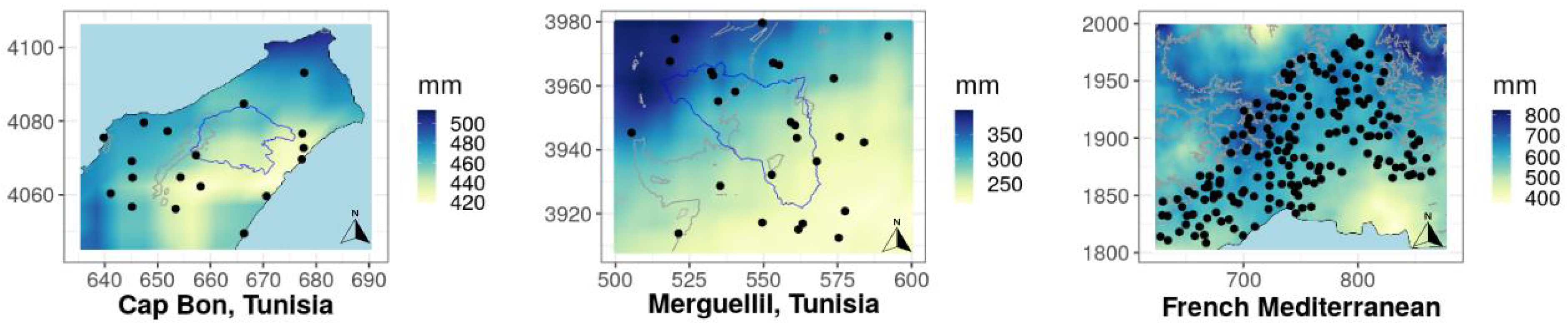
4.2. Spatial GEV Parameters Estimation

Two spatial tools have been proposed, acting as a bridge between local rainfall information to a smooth spatial mapping. For both models, the choice of covariates was made by 10-fold cross-validation (as explained in Section 3.2.2). The models are fitted for all possible combinations of the selected covariates (see row names of

Table 1. Validation error values for the GLM model resulted from the 10-fold cross-validation.

Covariate	French Mediterranean	Merguellil	Lebna
x	4341.18	488.39	364.70
y	4382.88	488.36	367.07
z	4341.94	488.46	366.97
chirps	4326.7	488.56	365.08
(x,y)	4305.67	487.34	361.42
(x,z)	4301.3	487.21	364.51
(y,z)	4340.35	488.63	363.98
(x,chirps)	4296.11	486.64	364.42
(y,chirps)	4313.43	487.00	364.65
(z,chirps)	4314.11	487.50	363.04
(x,y,z)	4275.84	486.52	360.75
(x,y,chirps)	4295.64	486.93	360.91
(y,z,chirps)	4301.79	487.46	361.89
(x,z,chirps)	4277.24	486.60	362.39
(x,y,z,chirps)	4274.04	486.55	361.25

). Validation error values that resulted from the cross-validation technique by fitting the GLM are presented in Table 1. For the ANN, there is an additional choice of the number of hidden units. We therefore have more validation errors to compare corresponding to the fitted ANN model with $nh=(0,1,2,4,6,8,12)$ hidden units. Results of covariate selection and the optimal number of hidden units for each region are summarized in

Table 2. The selected covariates for the spatial model (GLM and ANN) of the GEV parameters over the three sites. The number of hidden units concerns only the ANN model.

Site	GLM Covariate	ANN Covariate	Number of Hidden Units
French Mediterranean	(x,y,z,chirps)	(x,y,z,chirps)	4
Merguellil	(x,y,z)	(y,chirps)	1
Lebna	(x,y,z)	(y,z)	1

.

Results of the 10-fold cross-validation error curves by fitting the ANN model are presented in Appendix A.2. For the French Mediterranean site, we notice that the error curves do not rise with increasing the complexity level to 12 hidden units. According to the theory, the validation error curves tend to decrease until they reach a minimum and then increase again as we add complexity to the model. While performing some preliminary tests, we discovered that the data set is so large that we do not reach the overfitting area. Regarding the number of hidden units, the difference in terms of validation error is tiny, between 4 and 8 hidden units, so the optimal number was chosen where the descent stops (4 hidden units). We can also learn from these curves that using a unique covariate will give the worst models. So, it is recommended to select at least two covariates. When the four proposed covariates (x,y,z,chirps) are used simultaneously, the best model with the lowest validation error was obtained compared to the results produced by applying the other set of covariates. This finding emphasizes the interest in considering the climate variable CHIRPS. For both Tunisian regions, a single hidden unit corresponds to the model with the least errors. The selected covariates for the region of Merguellil are (y,chirps), and those for the Cap Bon region are (y,z). Compared with the French region, the model with the four covariates increases the error value, and that using two covariates is required to obtain a good performance.

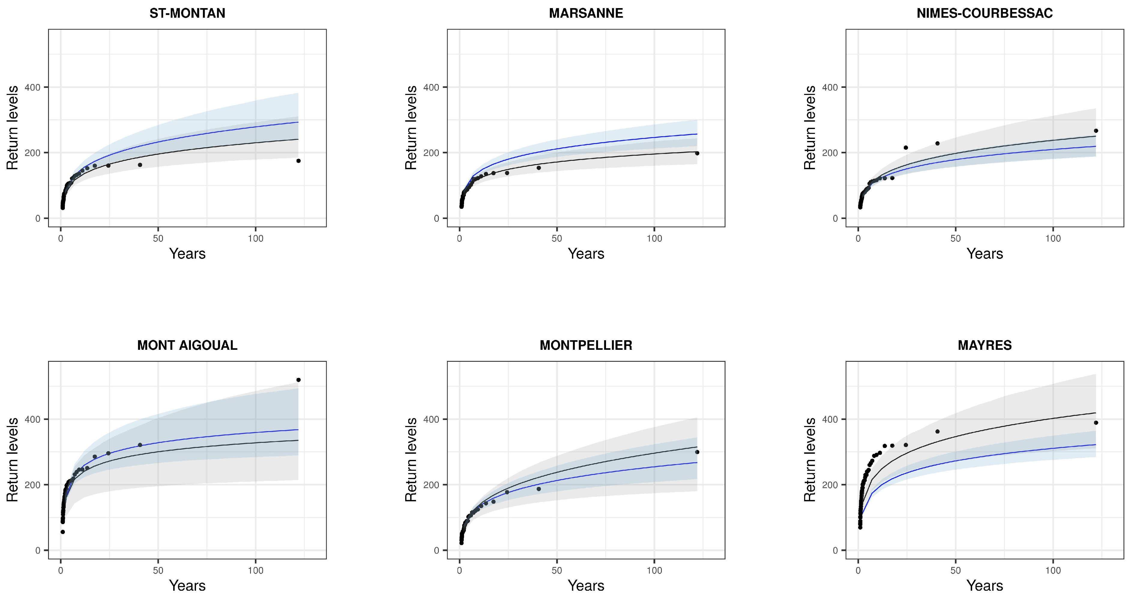
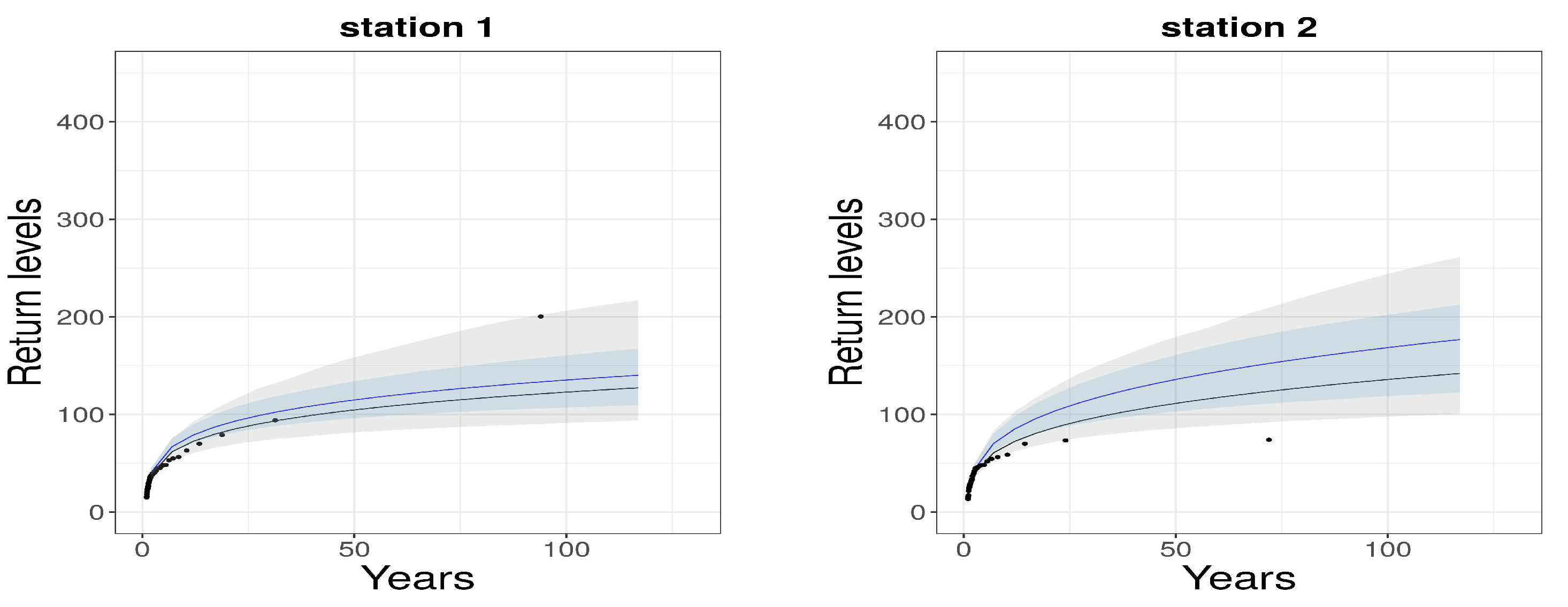
4.3. Model Evaluation

After selecting the covariates and the number of hidden units, we want to compare the two models (ANN versus GLM). For this purpose, negative log-likelihood values were calculated for each station and each study site. The number of stations that verified a minimum negative log-likelihood value with the neural network model was then calculated. The ratio over the total number of stations is given in

Table 3. The rate of the number of stations with a better performance with the ANN model.

Site	Negative Log-Likelihood	Kolmogorov–Smirnov
French Mediterranean	72.67%	74.35%
Merguellil	61.53%	65.38%
Lebna	61.1%	61.1%

. In addition, the goodness-of-fit was evaluated by the non-parametric Kolmogorov–Smirnov (Ks) test. The percentage of stations with a lower Ks distance using the ANN model was computed. These two values prove that the neural network model performs better on more than 60% of the stations compared to the GLM model.

To support this evaluation, we selected test stations (six stations for the French Mediterranean region and two stations for each Tunisian region) having a large number of observations and well distributed in space (see the stations depicted with red points in Figure 2). The Bootstrap resampling method was used to construct the 95% confidence bands of the return level curves. This technique was applied to both selected models (ANN and GLM) at the stations that were kept aside for testing. In total, 1000 replications were obtained by sampling with replacement years of annual maxima. The estimated return levels are represented by curves with the corresponding confidence bands. The evaluation consists of comparing the bands with the empirical return levels (black dots) based on observations.

For the French Mediterranean region, return level curves are presented in Figure 6. Confidence intervals represent the range of uncertainty associated with the estimate. The width of the GLM confidence intervals is narrow for most test stations compared to the ANN bands. In this case, the margin of error is smaller, and the model offers more precision. However, the GLM presents overestimation in St-Montan and Marsanne (stations 1 and 2, respectively, in Figure 2) or an underestimation in Nimes-courbessac and Mayres (station 3 and 6, respectively, in Figure 2) of the empirical estimates. Although the confidence bands are wider for the ANN, it can better capture empirical values.

For the Tunisian sites, return level curves are presented in Figure 7 and Figure 8. For these regions, the low density of the network of gauging stations implies that stations at the limit of the studied domain may suffer from a high estimation uncertainty because the regression model extrapolates outside its knowledge. The same evaluation process was applied to different selected test stations in each Tunisian region. An increase in the variation of the confidence bands was observed.

The test stations chosen in France have a complete number of observations, while in Capbon, we have an average of 19.29% of missing values on the two test stations (46.79% on all stations), and for Merguellil, we have an average of 46.3% of missing values (59.74% on all stations). The large number of stations in the French region, as well as the density of the hydro-meteorological station network, means that the model has more training data. This may affect the choice of model in terms of covariates and hidden units, which generates models with more accuracy when compared with the Tunisian data.

Given the difference between the results obtained for the French Mediterranean and Tunisia, a relationship was suspected between the density of the networks of the gauging station and the obtained results. It is certain that the quality of the data plays a major factor in the modeling. We performed a downgrading of the French dataset to become closer to the Tunisian dataset. For the French Mediterranean, the number of stations per 1000 km² is $6.57$, i.e., 1 station per 152 km². For Merguellil, the number of stations per 1000 km² is $3.6$, i.e., 1 station per 277 km². To have approximately the same density, we selected 100 stations instead of 183. The selection of covariates in this case for the ANN model is 4 hidden units and the covariates (x,y,z). We even attempted to take the same number of stations, i.e., 26 stations for the French Mediterranean region. In this case, the result of the cross-validation for the ANN model is to use (x,y,z,chirps) as covariates and 2 hidden units. From these experiments, we can deduce that there is a close relationship between model complexity and input size, which explains the difference between the number of hidden units in Table 2 (four for the French Mediterranean and one for each Tunisian site).

To review, the evaluation of the performance of the two models shows that the ANN model is considered to be more accurate than the GLM model for spatially approximating the risk of extreme events for these three study sites. The choice of covariates and the number of hidden units is different from one study site to another due to the difference in sample size as well as the difference in the inter-covariate association. By the 10-fold cross-validation, it was observed that the validation error is high when we fit a model with one covariate, and it is less obvious for two or more covariates.

In Figure 9, we present ANN spatial estimates within a radius of 15 km around the gauging stations of the French Mediterranean site. Pointwise estimates are illustrated by points for each station. The location and scale parameters show the highest values in the northwestern mountainous region, corresponding to the same variation in local estimates. For the shape parameter, a different spatial representation is shown with the highest values at the lowest altitude. Spatially, there are only positive values of the shape parameter, unlike the results of the local estimation. The results of the spatial estimation by ANN on the Tunisian sites are shown in Appendix A.1.

5. Discussion

In this work, we have emphasised the use of response surfaces for a smooth spatial representation of extreme events. This choice was motivated by the outcomes of [15,16]. It has been explicitly stated that it will be more efficient to bypass conventional spatial interpolation methods. Regional methods are more stable than methods based on spatial interpolation. It is of great benefit to take the surrounding area into account in order to ensure a smooth spatial variation of the parameters.

ANNs have proven their performance as a modern machine learning technique in several research areas and are gaining more and more popularity in hydrological studies. They overcome some of the weaknesses, such as linearity assumptions, of more classical methods. However, they are often seen as “black box” models in the sense that, while approximating a function, studying its structure will not provide any insight into the structure of the approximated function. Hence, the influence of each parameter estimate on covariates is difficult to interpret. For this purpose, it would be worth investigating the use of so-called interpretive machine learning (ML) models, where ANNs can be enhanced to highlight the understanding of relevant relationships in the data. For instance, the authors in [42,43] have built a flexible modeling framework by applying ML models to induce physically consistent models with high predictive accuracy. The idea is to combine a data-driven method (such as ANNs) with the understanding of physical process models: the training could be guided to mimic a physical phenomenon by specifying a physical law, serving as prior knowledge and added into the loss function.

Furthermore, we have focused on the analysis of extreme rainfall events that occur on a daily time scale. In fact, daily records are more widely available and usually exceed the length of the sub-daily observations. However, hydrological estimations often require long time series at high temporal resolution. The issue can be overcome by disaggregating daily into sub-daily values. Several resampling methods have been proposed to simulate a range of possible disaggregation scenarios that could occur at finer time scales. For example, non-parametric resampling models based on methods of fragments (MOF) (also called the analog method) have been shown to perform well compared to other disaggregation approaches [44,45]. In particular, [46] presented a space-time approach based on the MOF to convert daily-to-hourly precipitation. It would be interesting to follow up this idea by applying the proposed model to finer time scale data. Along the same lines, it would be interesting to perform a spatial estimation of the intensity–duration–frequency (IDF) curves in order to estimate the distribution of extreme precipitation of any duration at ungauged locations [47,48]. This could be seen as a starting point for building stochastic weather generators [49,50] that takes in account extreme events.

6. Conclusions

The main challenge of this work is to map the risk of extreme rainfall events taking into account spatial non-stationarity. To achieve this goal, two spatial estimation approaches are proposed to be applied to GEV parameters to assess the risk through the associated return levels. It has been shown that smooth spatial modeling by ANN gives better results on more than 60% of the stations compared to the GLM model.

One critical issue is to control the complexity level and the bias–variance trade-off. It was identified by optimizing the number of hidden neurons by a cross-validation method. Using a high variance model may not adequately capture the structure of the underlying phenomenon and become too dependent on training data. By contrast, a simpler model may lack flexibility and fail to capture the full complexity of the phenomenon. The trade-off between bias and variance occurs at the minimum of the generalization error.

The other issue concerns the choice of appropriate covariates that serve to add a geographical influence in the modeling of spatial non-stationarity. The CHIRPS climate variable is an effective source of information on the spatial distribution of rainfall. It was initially used in this study to compare the spatial behavior of observations. We checked the inter-annual totals of the gauging stations against the CHIRPS covariate, and we noticed that the local observations are globally higher than the CHIRPS rains, which is expected since it is an average over a 4 km grid. We included the CHIRPS data as a covariate with the geographical coordinates to provide a spatial description of the three Mediterranean regions.

References

1. Gaume, E.; Borga, M.; Llassat, M.; Maouche, S.; Lang, M.; Diakakis, M. Sub-chapter 1.3.4. Mediterranean extreme floods and flash floods. In The Mediterranean Region under Climate Change; Collection Synthèses; IRD Editions: Marseille, France, 2016; pp. 133–144. [Google Scholar] [CrossRef]
2. Leduc, C.; Ammar, S.B.; Favreau, G.; Beji, R.; Virrion, R.; Lacombe, G.; Tarhouni, J.; Aouadi, C.; Chelli, B.Z.; Jebnoun, N.; et al. Impacts of hydrological changes in the Mediterranean zone: Environmental modifications and rural development in the Merguellil catchment, central Tunisia/Un Ex. D’évolution Hydrol. En Méditerranée: Impacts Des Modif. Environnementales Et Du Développement Agric. Dans Le Bassin-Versant Du Merguellil (Tunisie Cent. Hydrol. Sci. J. 2007, 52, 1162–1178. [Google Scholar] [CrossRef]
3. Hmidi, N.; Fehri, N.; Baccar, A. Inondation devastatrice dans la ville de Soliman (Tunisie): Cas de sa zone industrielle lors de l’événement pluviométrique du 22 septembre 2018. In Le Changement Climatique, la Variabilité et les Risques Climatiques; AIC: Aix-en-Provence, France, 2019; p. 199. [Google Scholar]
4. Brunet, P.; Bouvier, C.; Neppel, L. Retour d’expérience sur les crues des 6 et 7 octobre 2014 à Montpellier-Grabels (Hérault, France): Caractéristiques hydro-météorologiques et contexte historique de l’épisode. Physio-Géo 2018, 12, 43–59. [Google Scholar] [CrossRef]
5. Katz, R.W.; Parlange, M.B.; Naveau, P. Statistics of extremes in hydrology. Adv. Water Resour. 2002, 25, 1287–1304. [Google Scholar] [CrossRef] [Green Version]
6. Coles, S. An Introduction to Statistical Modeling of Extreme Values; Springer Series in Statistics; Springer: Berlin/Heidelberg, Germany, 2001. [Google Scholar] [CrossRef]
7. Vicente-Serrano, S.M.; Saz-Sánchez, M.A.; Cuadrat, J.M. Comparative analysis of interpolation methods in the middle Ebro Valley (Spain): Application to annual precipitation and temperature. Clim. Res. 2003, 24, 161–180. [Google Scholar] [CrossRef] [Green Version]
8. Li, J.; Heap, A.D. A Review of Spatial Interpolation Methods for Environmental Scientists; Geoscience Australia: Canberra, Australia, 2008; p. 154.
9. Kumar Adhikary, S.; Muttil, N.; Gokhan Yilmaz, A. Ordinary kriging and genetic programming for spatial estimation of rainfall in the Middle Yarra River catchment, Australia. Hydrol. Res. 2016, 47, 1182–1197. [Google Scholar] [CrossRef]
10. Feki, H.; Slimani, M.; Cudennec, C. Incorporating elevation in rainfall interpolation in Tunisia using geostatistical methods. Hydrol. Sci. J. 2012, 57, 1294–1314. [Google Scholar] [CrossRef]
11. Feki, H.; Slimani, M.; Cudennec, C. Geostatistically based optimization of a rainfall monitoring network extension: Case of the climatically heterogeneous Tunisia. Hydrol. Res. 2017, 48, 514–541. [Google Scholar] [CrossRef]
12. Ceresetti, D.; Ursu, E.; Carreau, J.; Anquetin, S.; Creutin, J.D.; Gardes, L.; Girard, S.; Molinié, G. Evaluation of classical spatial-analysis schemes of extreme rainfall. Nat. Hazards Earth Syst. Sci. 2012, 12, 3229–3240. [Google Scholar] [CrossRef]
13. Shepard, D. A two-dimensional interpolation function for irregularly-spaced data. In Proceedings of the 1968 23rd ACM National Conference, New York, NY, USA, 27–29 August 1968; ACM Press: New York, NY, USA, 1968; pp. 517–524. [Google Scholar] [CrossRef]
14. Goovaerts, P. Geostatistical approaches for incorporating elevation into the spatial interpolation of rainfall. J. Hydrol. 2000, 228, 113–129. [Google Scholar] [CrossRef]
15. Blanchet, J.; Lehning, M. Mapping snow depth return levels: Smooth spatial modeling versus station interpolation. Hydrol. Earth Syst. Sci. 2010, 14, 2527–2544. [Google Scholar] [CrossRef] [Green Version]
16. Neppel, L.; Arnaud, P.; Borchi, F.; Carreau, J.; Garavaglia, F.; Lang, M.; Paquet, E.; Renard, B.; Soubeyroux, J.; Veysseire, J. Résultats du projet Extraflo sur la comparaison des méthodes d’estimation des pluies extrêmes en France. Houille Blanche-Rev. Int. L’eau 2014, 2, 14–19. [Google Scholar] [CrossRef] [Green Version]
17. Chowdhury, M.; Alouani, A.; Hossain, F. Comparison of ordinary kriging and artificial neural network for spatial mapping of arsenic contamination of groundwater. Stoch. Environ. Res. Risk Assess. 2010, 24, 1–7. [Google Scholar] [CrossRef]
18. Bishop, C.M. Pattern Recognition and Machine Learning; Information Science and Statistics; Springer: Berlin/Heidelberg, Germany, 2006. [Google Scholar]
19. Carreau, J.; Toulemonde, G. Extra-parametrized extreme value copula: Extension to a spatial framework. Spat. Stat. 2020, 40, 100410. [Google Scholar] [CrossRef] [Green Version]
20. Tramblay, Y.; Neppel, L.; Carreau, J.; Najib, K. Non-stationary frequency analysis of heavy rainfall events in southern France. Hydrol. Sci. J. 2013, 58, 280–294. [Google Scholar] [CrossRef]
21. Panthou, G.; Vischel, T.; Lebel, T.; Blanchet, J.; Quantin, G.; Ali, A. Extreme rainfall in West Africa: A regional modeling. Water Resour. Res. 2012, 48, 8. [Google Scholar] [CrossRef]
22. Šraj, M.; Viglione, A.; Parajka, J.; Blöschl, G. The influence of non-stationarity in extreme hydrological events on flood frequency estimation. J. Hydrol. Hydromech. 2016, 64, 426–437. [Google Scholar] [CrossRef] [Green Version]
23. Villarini, G.; Smith, J.; Serinaldi, F.; Ntelekos, A.; Schwarz, U. Analyses of extreme flooding in Austria over the period 1951–2006. Int. J. Climatol. 2012, 32, 1178–1192. [Google Scholar] [CrossRef]
24. Aissaoui-Fqayeh, I.; El-Adlouni, S.; Ouarda, T.B.M.J.; St-Hilaire, A. Non-stationary lognormal model development and comparison with the non-stationary GEV model. Hydrol. Sci. J. 2009, 54, 1141–1156. [Google Scholar] [CrossRef]
25. Wagner, P.D.; Fiener, P.; Wilken, F.; Kumar, S.; Schneider, K. Comparison and evaluation of spatial interpolation schemes for daily rainfall in data scarce regions. J. Hydrol. 2012, 464, 388–400. [Google Scholar] [CrossRef]
26. Slimani, M.; Cudennec, C.; Feki, H. Structure du gradient pluviométrique de la transition Méditerranée-Sahara en Tunisie: Déterminants géographiques et saisonnalité/Structure Rainfall Gradient Mediterranean-Sahara Transit. Tunisia: Geogr. Determ. Seas. Hydrol. Sci. J. 2007, 52, 1088–1102. [Google Scholar] [CrossRef]
27. Raymond, F. and Ullmann, A.; Tramblay, Y.; Drobinski, P.; Camberlin, P. Evolution of Mediterranean extreme dry spells during the wet season under climate change. Reg. Environ. Chang. 2019, 19, 2339–2351. [Google Scholar] [CrossRef]
28. Joly, D.; Brossard, T.; Cardot, H.; Cavailhes, J.; Hilal, M.; Wavresky, P. Les types de climats en France, une construction spatiale. Cybergeo 2010, 501, 34–42. [Google Scholar] [CrossRef]
29. Pujol, N.; Neppel, L.; Sabatier, R. Approche régionale pour la détection de tendances dans des séries de précipitations de la région méditerranéenne française. Comptes Rendus Geosci. 2007, 339, 651–658. [Google Scholar] [CrossRef]
30. Lacombe, G.; Cappelaere, B.; Leduc, C. Hydrological impact of water and soil conservation works in the Merguellil catchment of central Tunisia. J. Hydrol. 2008, 359, 210–224. [Google Scholar] [CrossRef]
31. Funk, C.; Peterson, P.; Landsfeld, M.; Pedreros, D.; Verdin, J.; Shukla, S.; Husak, G.; Rowland, J.; Harrison, L.; Hoell, A.; et al. The climate hazards infrared precipitation with stations-a new environmental record for monitoring extremes. Sci. Data 2015, 2, 150066. [Google Scholar] [CrossRef] [PubMed] [Green Version]
32. Fisher, R.A.; Tippett, L.H.C. Limiting forms of the frequency distribution of the largest or smallest member of a sample. Math. Proc. Camb. Philos. Soc. 1928, 24, 180–190. [Google Scholar] [CrossRef]
33. Pujol, N.; Neppel, L.; Sabatier, R. Regional tests for trend detection in maximum precipitation series in the French Mediterranean region. Hydrol. Sci. J. 2007, 52, 956–973. [Google Scholar] [CrossRef]
34. Cooley, D.; Nychka, D.; Naveau, P. Bayesian Spatial Modeling of Extreme Precipitation Return Levels. J. Am. Stat. Assoc. 2007, 102, 824–840. [Google Scholar] [CrossRef]
35. Hosking, J. L-moments: Analysis and Estimation of Distribution us sing Linear Combinations of Order Statistics. J. R. Stat. Soc. Ser. B Methodol. 1990, 52, 105–124. [Google Scholar] [CrossRef]
36. Hosking, J.R.M.; Wallis, J.R. Regional Frequency Analysis: An Approach Based on L-Moments, 1st ed.; Cambridge University Press: Cambridge, UK, 1997. [Google Scholar] [CrossRef]
37. McCullagh, P. Generalized Linear Models; Routledge: London, UK, 2019. [Google Scholar]
38. Chandler, R. On the use of generalized linear models for interpreting climate variability. Environmetrics 2005, 16, 699–715. [Google Scholar] [CrossRef]
39. Yan, Z.; Bate, S.; Chandler, R.E.; Isham, V.; Wheater, H. An Analysis of Daily Maximum Wind Speed in Northwestern Europe Using Generalized Linear Models. J. Clim. 2002, 15, 2073–2088. [Google Scholar] [CrossRef]
40. McCullagh, P.; Nelder, J.A. Generalized Linear Models; Monographs on statistics and applied probability; Chapman and Hall: New York, NY, USA, 1989. [Google Scholar]
41. Yee, T.W.; Stephenson, A. Vector generalized linear and additive extreme value models. Extremes 2007, 10, 1–19. [Google Scholar] [CrossRef]
42. Herath, H.; Chadalawada, J.; Babovic, V. Hydrologically informed machine learning for rainfall–runoff modelling: Towards distributed modelling. Hydrol. Earth Syst. Sci. 2021, 25, 4373–4401. [Google Scholar] [CrossRef]
43. Jiang, S.; Zheng, Y.; Wang, C.; Babovic, V. Uncovering flooding mechanisms across the contiguous United States through interpretive deep learning on representative catchments. Water Resour. Res. 2022, 58, e2021WR030185. [Google Scholar] [CrossRef]
44. Mezghani, A.; Hingray, B. A combined downscaling-disaggregation weather generator for stochastic generation of multisite hourly weather variables over complex terrain: Development and multi-scale validation for the Upper Rhone River basin. J. Hydrol. 2009, 377, 245–260. [Google Scholar] [CrossRef]
45. Carreau, J.; Mhenni, N.; Huard, F.; Neppel, L. Exploiting the spatial pattern of daily precipitation in the analog method for regional temporal disaggregation. J. Hydrol. 2019, 568, 780–791. [Google Scholar] [CrossRef]
46. Li, X.; Meshgi, A.; Wang, X.; Zhang, J.; Tay, S.H.X.; Pijcke, G.; Manocha, N.; Ong, M.; Nguyen, M.; Babovic, V. Three resampling approaches based on method of fragments for daily-to-subdaily precipitation disaggregation. Int. J. Climatol. 2018, 38, e1119–e1138. [Google Scholar] [CrossRef]
47. Mélèse, V.; Blanchet, J.; Creutin, J. A Regional Scale-Invariant Extreme Value Model of Rainfall Intensity-Duration-Area-Frequency Relationships. Water Resour. Res. 2019, 55, 5539–5558. [Google Scholar] [CrossRef]
48. Ulrich, J.; Jurado, O.; Peter, M.; Scheibel, M.; Rust, H. Estimating IDF Curves Consistently over Durations with Spatial Covariates. Water 2020, 12, 3119. [Google Scholar] [CrossRef]
49. Fatichi, S.; Ivanov, V.; Caporali, E. Simulation of future climate scenarios with a weather generator. Adv. Water Resour. 2011, 34, 448–467. [Google Scholar] [CrossRef]
50. Li, X.; Babovic, V. A new scheme for multivariate, multisite weather generator with inter-variable, inter-site dependence and inter-annual variability based on empirical copula approach. Clim. Dyn. 2019, 52, 2247–2267. [Google Scholar] [CrossRef]
Figure 1. Localization of the selected study areas around the Mediterranean region.
Water 14 03782 g001
Figure 2. DEMs for the three study sites. The selected stations are represented with average annual rainfall totals over rainy season represented by the blue scale. The stations numbered in red will serve as test stations. The sky blue area represents the Mediterranean Sea and the blue lines delimit the catchment areas.
Water 14 03782 g002
Figure 3. Interpolated average seasonal precipitation totals computed from the CHIRPS data constituting the CHIRPS spatial covariate. The gauging stations are depicted as black points, and contour lines from DEM are represented by the gray lines.
Water 14 03782 g003
Figure 4. Kendall’s correlation matrix for the covariates corresponding to the three study areas.
Water 14 03782 g004
Figure 5. Box−plots of estimated L-moments parameters of GEV distribution ( μ , σ , ξ ) and 100-year return level.
Water 14 03782 g005
Figure 6. Return levels at the selected test stations for the French Mediterranean region. The 95% bootstrap confidence bands of the return levels obtained from the fitted models: the ANN in gray and the GLM in blue. The dots represent the empirical return levels.
Water 14 03782 g006
Figure 7. Return levels at the selected test stations for the Merguellil region, showing 95% bootstrap confidence bands of the return levels obtained from the fitted models: the ANN in gray and the GLM in blue. The dots represent the empirical return levels.
Water 14 03782 g007
Figure 8. Return levels at the selected test stations for the Cap Bon region, showing 95% bootstrap confidence bands of the return levels obtained from the fitted models: the ANN in gray and the GLM in blue. The dots represent the empirical return levels.
Water 14 03782 g008
Figure 9. Estimates of the GEV parameters ( μ , σ , ξ ) and the 100-year return level over the French Mediterranean region. Spatial estimates result from an ANN using (x,y,z,chirps) as covariates with four hidden units, and the point estimations are obtained by the L−moments method.
Water 14 03782 g009