The Large-Scale Hydraulic Conductivity for Gravitational Fingering Flow in Unsaturated Homogenous Porous Media: A Review and Further Discussion

Abstract

Gravitational fingering often occurs for water flow in unsaturated porous media. This paper reviews a recent effort in developing a macroscopic theory to describe the gravitational fingering flow of water in homogeneous and unsaturated soils, based on the optimality principle that water flows in unsaturated soils in such a manner that the generated flow patterns correspond to the minimum global flow resistance. The key difference between the new theory and the conventional unsaturated flow theories is that the hydraulic conductivity in the new theory is not only related to water saturation or capillary pressure, but also proportional to a power function of water flux, because the water flux is closely related to the fingering flow patterns and the power function allows for large hydraulic conductivities at locations where water fluxes are large as well to minimize the global flow resistance. The resultant relationship for the fraction of fingering flow zone is compared with that obtained from a parallel effort based on the fractal nature of fingering flow patterns. The relationships from the two efforts are found to be essentially identical for gravity-dominated water flow in unsaturated soils and can both be expressed as a power function of the water saturation. This work also demonstrates that the theoretical values for the exponent of the power function vary in a relatively narrow range between 0.75 and 0.80 for most soils, which is supported by observations from previous field tests. This remarkable finding makes it easy to apply the new theory to field sites where experimental data are not readily available for estimating the exponent value. The potential limitations of the theory and the suggested future research topics in the area are also discussed.

1. Introduction

Downward water flow in unsaturated soils is often associated with so-called preferential flow that is nonuniform, can by-pass significant portion of soils, and thus results in rapid water flow and solute transport from the ground surface to the water table for a given water flux at the ground surface [1]. Preferential flow has been a major research area in the vadose zone hydrology community and probably considered the most frustrating processes in terms of hampering accurate predictions of contaminant transport in the vadose zone [2]. There are two major mechanisms for the preferential flow. One is the existence of soil macropores near the ground surface that give rise to fast water flow within these pores that are not in the hydraulic equilibrium with surrounding soil matrix [3,4]. Water flow process in soils within macropores is similar to the process in unsaturated fractured rock, with the macropores playing essentially the same role as fractures [5,6]. The other major mechanism is gravitational fingering flow resulting from soil–water wetting front instability during the infiltration process [7,8,9,10]. While field-scale preferential flow is likely caused by a combination of the two mechanisms, how to accurately model the flow process in a theoretically rigorous way remains a technical challenge [11].

This paper focuses on fingering flow in unsaturated and homogeneous soils because of gravitational instability. Fingering flow likely plays a more important role in the deep vadose zone while macropores often exist near the ground surface only. There are two scales associated with the fingering flow (Figure 1). The local scale is characterized by a size considerably smaller than the width of a water finger. On this scale, the traditional Darcy–Buckingham law applies [10], because of the validity of the local equilibrium assumption that water capillary pressure is essentially uniform across the scale under consideration and thus water distribution is purely determined by the pore size distribution. The Darcy–Buckingham law was developed based on the local equilibrium assumption. Under the local equilibrium, the local-scale hydraulic conductivity is fully determined by water capillary pressure or saturation [12,13]. Note that the so-called local scale herein may also be considered to correspond to a small grid block in a continuum-based numerical model. In other words, the traditional Darcy–Buckingham law can be used for modeling fingering flow with very fine numerical grid systems, which, however, is very computationally intensive and may not be realistic in the foreseeable future for field-scale problems [10].

The other scale is called large scale, or macroscale, which corresponds to a coarse grid block including multiple fingers within it (Figure 1). At the large scale, the local equilibrium assumption is not valid simply because the water capillary pressure is not uniform across the scale (or the course grid block). The water capillary pressures can be significantly different between the water fingers and the nonfingering zone (Figure 1). Consequently, water distribution within the grid block cannot be purely determined by the pore size distribution but is related to the flow pattern. In this case, the traditional Darcy–Buckingham law is not applicable, and an additional physical principle needs to be introduced for characterizing the flow pattern. Since models with coarse grid blocks are more useful in practical applications, it is highly desirable to develop a large-scale relationship for hydraulic conductivities for modeling fingering flow processes.

Recently, an effort has been made to investigate the large-scale hydraulic conductivity for modeling fingering flow processes by incorporating an additional physical principle or so-called optimality [10,14]. The optimality principle refers to the state of a physical process that is controlled by an optimal condition subject to physical and resource constraints [14]. Different versions of the principle have been used in several areas, including evolution of vegetation coverage under water-limited conditions [15] and tree-like pathways for liquid flow and heat transfer [16]. The importance of the optimality principle in forming complex natural flow patterns, such as water channels, has been recognized and intensively studied for many years in the surface hydrology communities [17,18,19,20]. However, the quantitative applications of the optimality to subsurface flow problems are very limited probably because flow patterns in the subsurface are difficult to observe and characterize.

Based on the optimality principle that water flows in unsaturated porous media in such a manner that the generated flow patterns correspond to the minimum global flow resistance, Liu [10,14] mathematically derived a large-scale relationship of hydraulic conductivity for the fingering flow process. The hydraulic conductivity has been found to be a function of not only water saturation or capillary pressure, but also water flux. The consistency between the theoretical relationship and laboratory and field observations was demonstrated as well [10,14]. In a parallel effort, Liu et al. also developed a large-scale relationship of hydraulic conductivity based on the fractal nature of fingering flow patterns [21].

The objectives of this work are to review the development of large-scale relationships of hydraulic conductivity for the fingering flow process, demonstrate the consistency of theoretical results obtained based on both optimality and fractal flow patterns, and present typical values for key parameters in the large-scale relationship that is especially important for practical applications.

2. Theory

This section discusses large-scale relationships of hydraulic conductivity for the fingering flow processes, based on both the optimality and fractal flow patterns, and their consistency.

2.1. The Relationship Based on the Optimality Principle

As previously indicated, Darcy–Buckingham law was developed based on the local equilibrium assumption and an additional physical principle is needed for deriving the large-scale relationship of hydraulic conductivities for the fingering flow process. We here present the detailed procedure to obtain such a relationship based on the optimality principle that water flows in unsaturated porous media in such a manner that the generated flow patterns correspond to the minimum global flow resistance. 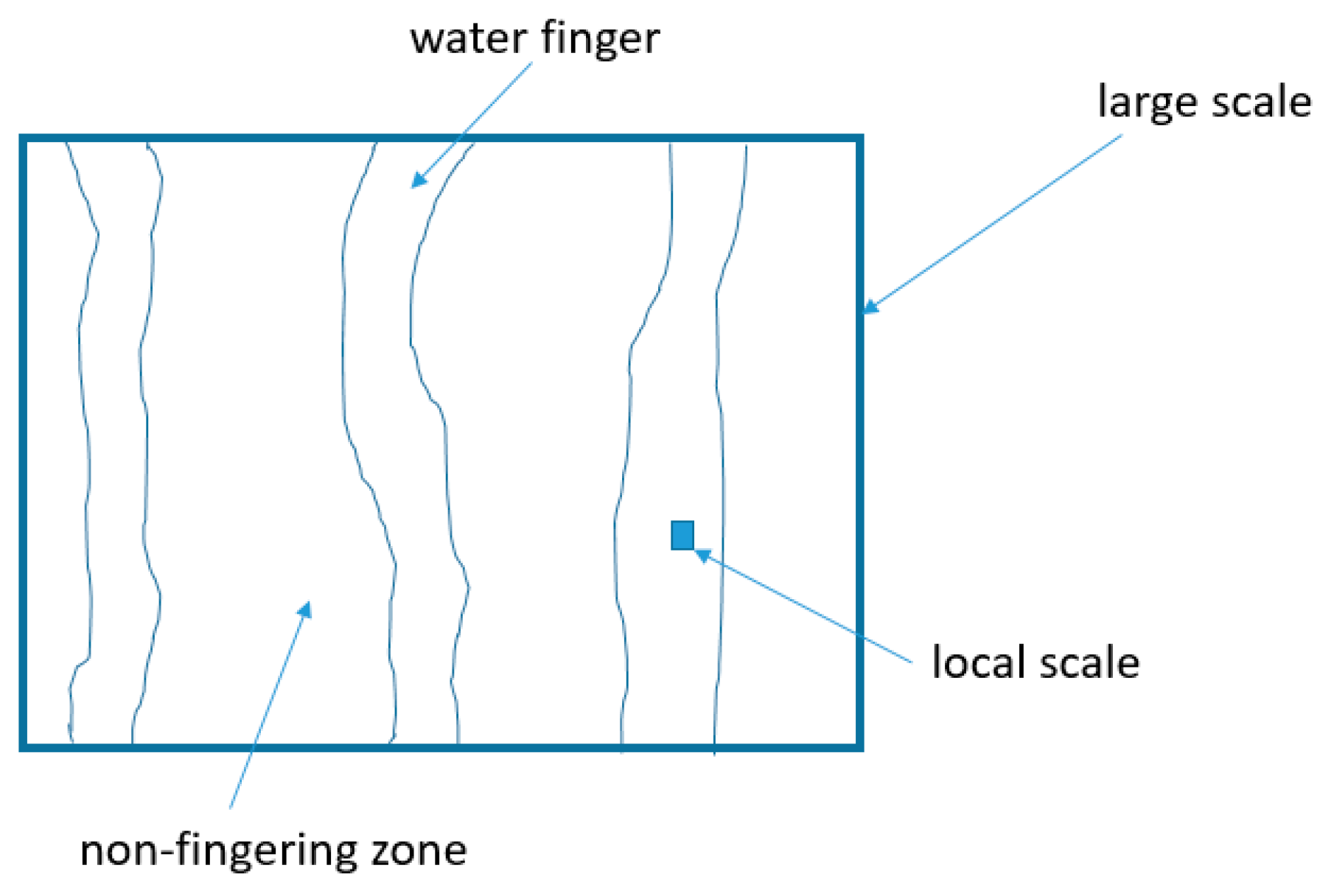Following the common practice to determine large-scale flow parameters [22], we focus on the steady-state flow process given that this work focuses on the fully developed fingering flow process. The steady-state water flow equation on a large scale (Figure 1) for a homogeneous and isotropic porous medium is given as

$$\frac{\partial q_x}{\partial x}+\frac{\partial q_y}{\partial y}+\frac{\partial q_z}{\partial z}=0$$

(1)

where x and y are the two horizontal coordinate axes, z is the vertical axis, and q_x, q_y and q_z are large-scale Darcy flux along x, y and z directions, respectively.

To apply the optimality principle, we need to derive the expression for energy expenditure rate. The energy of unit weight of liquid water in a porous medium, E, is given by

$$E=z+h$$

(2)

where h is the average capillary pressure head within the fingers as shown in Figure 1. The energy expenditure rate for a unit volume of porous medium can be written as

$${\Delta }_E=\frac{\partial \left(q_{x}E\right)}{\partial x}+\frac{\partial \left(q_{y}E\right)}{\partial y}+\frac{\partial \left(q_{z}E\right)}{\partial z}$$

(3)

The above equation represents the rate of water energy loss within a unit volume of porous medium. Combining Equations (1) and (3) yields

$${\Delta }_E=q_x\frac{\partial E}{\partial x}+q_y\frac{\partial E}{\partial y}+q_z\frac{\partial E}{\partial z}$$

(4)

Therefore, the rate of water energy loss is represented by a product of water flux and energy gradient.

Following Liu [10,14], we assume that the mathematical form of Darcy–Buckingham law is still applicable to the fingering process at a large scale except that the corresponding hydraulic conductivity, as discussed below, does not depend on water saturation or capillary pressure only:

$$q_x=-K\frac{\partial E}{\partial x}; q_y=-K\frac{\partial E}{\partial y}; q_z=-K\frac{\partial E}{\partial z}$$

(5)

The major difference between Liu [10,14] and the traditional unsaturated flow theories is the expression for hydraulic conductivity K. Conventionally, K is a function of water saturation or capillary pressure only. This is a direct result of the local equilibrium assumption that, however, is not valid for modeling fingering flow on a large scale. In other words, the water distribution within a course grid block (Figure 1) cannot be uniquely determined by water saturation or capillary pressure alone. Additional large-scale variables are needed to accurately determine the state of subgrid water distribution. Water flux is a logical choice because it is highly relevant to the fingering flow process. Following Liu [10,14], we used the square of the energy gradient as the additional variable to determine the large-scale conductivity for mathematical convenience. This is equivalent to the use of water flux because water flux and the energy gradient are related to each other (Equation (5)). In this case, the large-scale hydraulic conductivity is given by

$$K=K_{sat}{k}_r\left(h,S_{*}\right)$$

(6)

where K_sat is the saturated hydraulic conductivity, $k_r$ is the relative permeability, and the square of the energy gradient $S_{*}$ is defined by

$$S_{*}={\left(\frac{\partial E}{\partial x}\right)}^2+{\left(\frac{\partial E}{\partial y}\right)}^2+{\left(\frac{\partial E}{\partial z}\right)}^2$$

(7)

The optimality principle is used to derive the explicit relationship among K, h, and $S_{*}$ (Equation (6)). Based on Equations (4), (5), and (7), we can write the total energy expenditure rate for the whole flow domain as

$$\int \int \int {\Delta }_{E}dxdydz=\int \int \int \left(-K{S}_{*}\right)dxdydz$$

(8)

When applying the optimality principle regarding the minimization of global flow resistance, the total energy expenditure rate could be either the minimum or the maximum, depending on the given boundary conditions. For fixed E values at boundaries, the small flow resistance will allow for large water flux and thus the absolute value of the energy expenditure rate will reach its maximum. On the other hand, for fixed flux values at boundaries, the small flow resistance will allow for small absolute values of the energy gradient along the flow path and thus the absolute value of the energy expenditure rate will reach its minimum. These are the direct results of the definition of the energy expenditure rate that is the product of water flux and energy gradient. This important relation between boundary conditions and the extrema of the total energy expenditure rate was not discussed in Liu [10,14]. In this work, we used the boundary conditions with fixed E values, which, as demonstrated later, allows for deriving mathematically tractable results.

The calculus of variations is used here to deal with the extremum problems of Equation (8). While we encourage readers to consult the relevant mathematical textbooks on the details of calculus of variations [23], some of the results used in this study are briefly presented here. Consider a functional I_w with an unknown function w:

$$I_w=\int \int \int L\left(x,y,z,w,w_x,w_y,w_z\right)dxdydz$$

(9)

where function L is called Lagrangian, and w_x, w_y, and w_z are derivatives of w with respect to x, y, and z, respectively. When I_w reaches its extrema, the unknown function w follows the Euler equation [23]:

$$\frac{\partial L}{\partial w}-\frac{\partial }{\partial x}\left(\frac{\partial L}{\partial w_x}\right)-\frac{\partial }{\partial y}\left(\frac{\partial L}{\partial w_y}\right)-\frac{\partial }{\partial z}\left(\frac{\partial L}{\partial w_z}\right)=0$$

(10)

Then, Equation (10) can be used to solve function w. The above form of the Euler equation holds only when w has fixed values or satisfies the following condition at boundaries:

$$\frac{\partial L}{\partial w_x}=\frac{\partial L}{\partial w_y}=\frac{\partial L}{\partial w_z}=0$$

(11)

Equations (9) and (10) were developed only for a functional with one unknown function. For cases with more than one unknown functions, Equation (10) was applied to each one of these functions [23].

From Equation (8), we have the Lagrangian function

$$L=-K{S}_{*}+{\lambda }^{\prime }\left[S_{*}-{\left(\frac{\partial E}{\partial x}\right)}^2-{\left(\frac{\partial E}{\partial y}\right)}^2-{\left(\frac{\partial E}{\partial z}\right)}^2\right]$$

(12)

The second term on the right-hand side of the above equation is a constraint from Equation (7). The Lagrange multiplier ${\lambda }^{\prime }$ is a function. The constraint related to the water flow equation (Equation (1)) is not included in Equation (12) and handled later.

Since $S_{*}$ satisfies Equation (11), Equation (10) is applicable when replacing w with $S_{*}$. Inserting Equation (12) into Equation (10) gives:

$${\lambda }^{\prime }=\frac{\partial \left(K{S}_{*}\right)}{\partial S_{*}}$$

(13)

In this study, we considered a boundary condition with fixed E values at boundaries. Thus, Equation (10) is also applicable when replacing w with E. Inserting Equation (12) into Equation (10) and using Equations (1) and (13) yield:

$$\frac{\partial \left(\frac{\partial K}{\partial \left(log{S}_{*}\right)}\frac{\partial E}{\partial x}\right)}{\partial x}+\frac{\partial \left(\frac{\partial K}{\partial \left(log{S}_{*}\right)}\frac{\partial E}{\partial y}\right)}{\partial y}+\frac{\partial \left(\frac{\partial K}{\partial \left(log{S}_{*}\right)}\frac{\partial E}{\partial z}\right)}{\partial z}=\frac{S_{*}}{2}\frac{\partial K}{\partial h}$$

(14)

While Liu [10,14] also obtained Equations (13) and (14) with the Euler equation (Equation (10)), he did not clearly specify the boundary conditions for E and $S_{*}$. As previously indicated, specific boundary conditions are required for applying Equation (10).

As indicated by Liu [10,14], an analytical relationship for the large-scale hydraulic conductivity can be obtained if the term on the right-hand side of Equation (14) becomes zero. Liu [14] argued that for a gravity-dominant flow the term on the right-hand side of Equation (14) is small based on a rough order-of-magnitude analysis [S(∂K/∂h)]/(∂K/∂logS) = ∂S/∂h. For a gravity-dominant flow, the energy gradient is close to one in the vertical direction and not a strong function of local capillary pressure at locations occupied by flow patterns. In other words, for two different gravity-dominated flow situations for a given flow system, changes in the energy gradient are much smaller than changes in the capillary pressure. This argument is also consistent with an observation that ∂K/∂h → 0 for large water saturation (corresponding to the gravity-dominated conditions) [13]. In this case, the term on the right-hand side of Equation (14) drops and then that equation becomes

$$\frac{\partial \left(\frac{\partial K}{\partial \left(log{S}_{*}\right)}\frac{\partial E}{\partial x}\right)}{\partial x}+\frac{\partial \left(\frac{\partial K}{\partial \left(log{S}_{*}\right)}\frac{\partial E}{\partial y}\right)}{\partial y}+\frac{\partial \left(\frac{\partial K}{\partial \left(log{S}_{*}\right)}\frac{\partial E}{\partial z}\right)}{\partial z}=0$$

(15)

Note that Equation (1) can be rewritten as

$$\frac{\partial \left(K\frac{\partial E}{\partial x}\right)}{\partial x}+\frac{\partial \left(K\frac{\partial E}{\partial y}\right)}{\partial y}+\frac{\partial \left(K\frac{\partial E}{\partial z}\right)}{\partial z}=0$$

(16)

Equation (15) provides the partial differential equation that K should satisfy based on the optimality principle. However, the derivation of Equation (15) does not consider the constraints of the water flow equation (Equation (1) or (16)), as previously indicated. A comparison between Equations (15) and (16) indicates that the water flow equation (Equation (16)) is also satisfied if we let

$$\frac{\partial K}{\partial \left(\log S_{*}\right)}=AK$$

(17)

where $A$ is a constant.

Following Liu [14], we approximately express K by

$$K=K_{sat}{k}_r\left(h,S_{*}\right)=K_{sat}{f}_h\left(h\right)g_s\left(S_{*}\right)$$

(18)

where $f_h$ and $g_s$ are functions of h and $S_{*}$, respectively. Inserting Equation (18) into Equation (17) results in

$$g_s\left(S_{*}\right)\propto {\left(S_{*}\right)}^A$$

(19)

Based on Equation (5), the above equation can be rewritten as

$$g_s\left(S_{*}\right)\propto {\left(\frac{q}{K_{sat}}\right)}^{A/2}$$

(20)

where q is the magnitude of water flux given by

$$q={\left(q_x^2+q_y^2+q_z^2\right)}^{1/2}$$

(21)

Inserting Equation (20) into Equation (18) gives the final relationship of large-scale hydraulic conductivity for gravitational fingering flow in unsaturated homogeneous porous media as

$$K=K_{sat}{F}_h\left(h\right){\left(\frac{q}{K_{sat}}\right)}^a$$

(22)

where F_h is a function of h and a is a constant. The term $K_{sat}{F}_h\left(h\right)$ in Equation (22) is considered unsaturated hydraulic conductivity on a local scale (Figure 1) simply because it is a function of h (the capillary pressure head in fingering flow zone) only. The power function term

$$f={\left(\frac{q}{K_{sat}}\right)}^a$$

(23)

represents the fraction of fingering flow zone in the cross section normal to the flux direction [10,14]. Wang et al. compiled laboratory experimental results of gravitational fingering flows and found the same relationship for the fraction of fingering flow zone with a = 0.5 [8].

The fact that the large-scale hydraulic conductivity is a function of flux, as shown in Equation (22), is consistent with behavior of other unstable flow processes, such as turbulent flow. To be more specific, Liu compared Equation (22) to the expression of water viscosity in the literature of hydrodynamics, with the conductivity and viscosity being considered as conceptual analogues [10]. He considered laminar water flow and turbulent flow within the context of hydrodynamics to correspond to unform flow (or nonfingering flow) in unsaturated soils and fingering flow, respectively, for comparison purposes. As the hydraulic conductivity is only a function of water saturation in the uniform flow in unsaturated soils, the water viscosity in the laminar flow is a sole property of water and not associated with water velocity. However, for turbulent flows, the apparent viscosity is related to the Reynolds number (Re) that is a function of water velocity. Consequently, it should not be surprising that conductivity for fingering flow depends on water flux because both fingering flow in unsaturated soils and water turbulent flow in hydrodynamics conceptually belong to the same flow regime in a broad sense: unstable flow. Furthermore, as there are different constitutive models for water flow in laminar and turbulent flow regimes in the hydrodynamics community, we need to develop the theoretical framework for large-scale fingering flow, in addition to the framework of uniform flow (Darcy–Buckingham law), to fully describe soil water flow in all the regimes. Our work is only the initial step to address this significant issue.

For a positive a value, Equation (22) indicates that large conductivity values correspond to locations where water fluxes are large as well, so that the global flow resistance is minimized. This is also consistent with our daily life experiences. For example, to maximize traffic transportation efficiency, our highways always have more lanes in locations with high-traffic fluxes. Highway networks may be analogous to fingering flow paths, with traffic flux and the number of lanes corresponding to water flux and hydraulic conductivity, respectively. Liu noted that when the conductivity for a flow system is defined as the flux divided by the absolute value of energy gradient, the power relationship between the conductivity and the flux exists for different flow systems, including water flow in a river basin and heat flow in the Earth’s climate system [10]. Further discussion of these flow systems is beyond the scope of this paper and readers are referred to Liu [10] for the details of them. Nevertheless, the existence of the power relationship among different flow systems implies that such a relationship could be a signature of highly nonlinear flow systems, although the exponents are different for different flow systems simply because these systems are subject to different flow mechanisms.

2.2. The Relationship Based on the Fractal Flow Pattern

In Section 2.1, we derived a large-scale relationship of hydraulic conductivity for the fingering flow process based on the optimality principle. As a parallel effort, a large-scale relationship was also derived from a more “descriptive” point of view by incorporating the fractal nature of fingering flow patterns [21]. This subsection provides the detailed derivation of the relationship based on the fractal flow patterns, while Section 2.3 will demonstrate that the two relationships are essentially equivalent for gravitational fingering flow in unsaturated soils.

Several researchers reported the observed fractal patterns of fingering flow in unsaturated soils. For example, Flury and Flühler [24] and Persson et al. [25] indicated that solute leaching patterns, characterizing fingering flow in fields, can be well modeled with a diffusion-limited aggregation (DLA) method that is known to generate fractal patterns [26]. Closely related to water flow process in unsaturated soils, fractal flow patterns are also observed from multiphase flow systems. Again, as an example, Smith and Zhang reported that gravitational DNAPL (dense nonaqueous phase liquid) fingering flow in water saturated porous media, observed from sandbox experiments, was fractal [27].

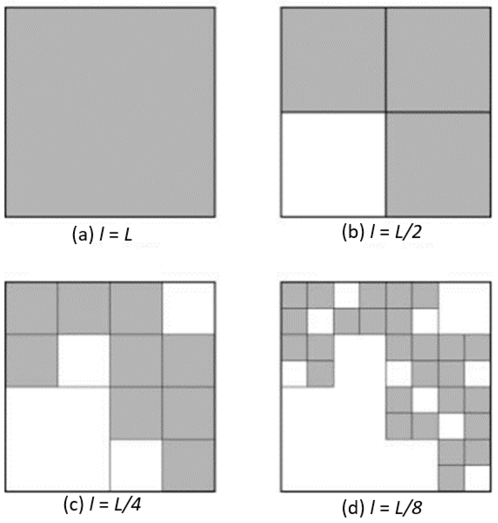
A fractal pattern is characterized by the so-called fractal dimension, $d_f$, that is generally not an integer and smaller than the corresponding Euclidean (topological) dimension of the space, D. There are different ways to determine fractal dimensions in practice. One straightforward definition of the fractal dimension is called “box” dimension that is determined by counting the number (N) of box, as a function of box size (l), required to cover the fractal pattern:

$$N\left(l\right)={\left(\frac{L}{l}\right)}^{df}$$

(24)

where L is the characteristic size of the fractal pattern beyond which fractal behavior may not exist any longer. Note that in practice the fractal only exists on a limited range of scales and not on all length scales. For example, Figure 2 shows the “box” counting procedure for a two-dimensional fingering flow pattern with a fractal dimension of 1.6.

For the uniform flow pattern, the box dimension will be the same as the Euclidean (topological) dimension of the space, D. In this case, the number of box (N*) with a size l to cover the flow pattern with the characteristic size L is

$$N^{*}\left(l\right)={\left(\frac{L}{l}\right)}^D$$

(25)

From Equations (24) and (25), we have

$$\frac{L}{l}=N{\left(l\right)}^{\frac{1}{df}}=N^{*}{\left(l\right)}^{\frac{1}{D}}$$

(26)

The average effective water saturation for the “box” with size L is estimated by

$$S_e=\frac{V_w}{l^D\phi N^{*}\left(l\right)}$$

(27a)

where $V_w$ is the total volume of the mobile water within the box, $\phi$ is porosity, and S_e is effective water saturation defined by

$$S_e=\frac{\theta -{\theta }_r}{{\theta }_{sat}-{\theta }_r}$$

(27b)

where $\theta$ is water content, ${\theta }_r$ is the residual water content, and ${\theta }_{sat}$ is the saturated water content and should be equal to the porosity when there is no trapped air. Similarly, the average effective water saturation for the fractal flow pattern within the “box” with size L is given by

$$S_f=\frac{V_w}{l^D\phi N\left(l\right)}$$

(28)

Obviously, $S_f$ is always larger than $S_e$.

Since the porous medium is under the unsaturated condition, we can always find a length scale $l_1<L$ such that

$$\frac{V_w}{l_1^D\phi }=1$$

(29)

Thus, for $l=l_1$, we have from Equations (27) and (28):

$$S_e=\frac{1}{N^{*}\left(l_1\right)}$$

(30)

and

$$S_{f,1}=\frac{1}{N\left(l_1\right)}$$

(31)

Inserting the above two equations into Equation (26) yields

$$S_{f,1}={\left(S_e\right)}^{\frac{df}{D}}$$

(32)

In the above discussion, we have developed a saturation relationship (Equation (32)) for a control volume (or “box”) with a characteristic length L and a cutoff scale l₁. However, a nonequilibrium process may still exist on the scale l₁. Thus, we continue the process for deriving Equation (32), on an average sense, for a smaller control volume with a characteristic length l₁ and a cutoff scale l₂ < l₁ at which we have:

$$\frac{V_{w,1}}{l_2^D\phi }=1$$

(33)

where V_w,1 is the average water volume for the small control volumes covering the fingering flow part and determined by $V_w/N^{*}\left(l_1\right)$.

Following the same mathematical procedure to derive Equation (32), we obtain the following saturation relationship:

$$S_{f,2}={\left(S_{f,1}\right)}^{\frac{df}{D}}={\left(S_e\right)}^{{\left(\frac{df}{D}\right)}^2}$$

(34)

We continue the above process for the smaller and smaller cutoff scales until the scale reaches $l_{n-1}$ at which the local equilibrium starts to hold. In this case, we have

$$S_f=S_{f,n}={\left(S_e\right)}^{{\left(\frac{df}{D}\right)}^n}$$

(35)

Note that Equation (35) holds only for a series of discrete cutoff scales $l_{n-1}$ (n = 2, 3, …). However, Equation (35) can hold approximately for a length scale between the two adjacent cutoff scales if n is allowed to take noninteger values. Thus, Equation (36) is practically general for fingering flow pattens.

Using the definition of the fraction of fingering flow zone, we have:

$$f=\frac{S_e}{S_f}=S_e{}^{\gamma }$$

(36)

where

$$\gamma =1-{\left(\frac{df}{D}\right)}^n$$

(37)

Note that $d_f=D$ corresponds to the uniform flow or f = 1. Equations (36) and (37) imply that the traditional theory is not able to capture the fingering flow on a macroscopic or large scale because the theory ignores the difference between the fractal dimension of the fingering flow pattern and the topological dimension of the space. This dimension difference is the other way to state that the local equilibrium does not hold any longer on a macroscopic scale when fingering flow occurs (Figure 1).

In Equation (37), fractal dimension $d_f$ and parameter n are difficult to determine in practice. The parameter n is determined by L, the characteristic size of a fractal pattern beyond which fractal behavior may not exist any longer, and length scale $l_{n-1}$ at which the local equilibrium starts to hold. Liu et al. suggested to treat parameter $\gamma$ as a constant for practical applications and the first step to incorporate the dimension difference [21]. The validity of this suggestion and typical $\gamma$ values for unsaturated soils will be discussed later. Additionally, based on Equation (36), one can easily obtain the large-scale hydraulic conductivity for the gravitational fingering flow that is simply the local-scale conductivity (associated with average water saturation within the fingers) multiplied by the fraction of fingering flow zone f.

2.3. The Consistency between the Relationships Derived from the Two Methods

The two relationships of the large-scale hydraulic conductivity for gravitational fingering flow have been derived based on the optimality principle and the fractal behavior of the fingering flow patterns, respectively. We demonstrate that the two relationships are consistent at least in an approximate sense.

Firstly, we show that the expression for the fraction of fingering flow zone, obtained from the fractal fingering flow patterns, can also be derived from the results based on the optimality principle. For the gravity-dominated flow, the hydraulic gradient is approximately equal to one. Consequently, the magnitude of the vertical flux, q, is equal to the hydraulic conductivity, or

$$q=K_{f}f$$

(38)

where K_f is hydraulic conductivity within the fingering zone. Inserting Equation (38) into Equation (23) gives

$$f={\left(\frac{K_{f}f}{K_{sat}}\right)}^a$$

(39)

Note that $K_f/K_{sat}$ is the relative permeability within the fingering zone and can be represented with Brooks–Corey relation [12]:

$$\frac{K_f}{K_{sat}}={\left(S_f\right)}^{\beta }={\left(\frac{S_e}{f}\right)}^{\beta }$$

(40)

where $\beta$ is a constant defined by [12]

$$\beta =\frac{2+3\lambda }{\lambda }$$

(41)

where $\lambda$ is the index for the pore-size distribution.

Inserting Equation (40) into Equation (39) and solving for f, we obtain Equation (36) with the exponent $\gamma$ defined by

$$\gamma =\frac{a\beta }{1+a\beta -a}$$

(42)

Since we can derive Equation (36), a result obtained based on the fractal flow patterns, from the large-scale hydraulic conductivity derived based on the optimality principle, the two relationships from the two methods are consistent. Additionally, Equation (42) indicates that parameter $\gamma$ is a constant, implying that the suggestion of Liu et al. [21] to treat $\gamma$ as a constant seems to be valid.

One interesting question is what the typical $\gamma$ values are for most unsaturated soils. The answer is especially important for some practical applications in which values for $\gamma$ are not readily available from experimental observations. Fortunately, Equation (42) provides a way to estimate theoretical values for $\gamma$. As previously indicated, Wang et al. compiled laboratory experimental results and found a = 0.5 [8] that is used herein for estimating $\gamma$. 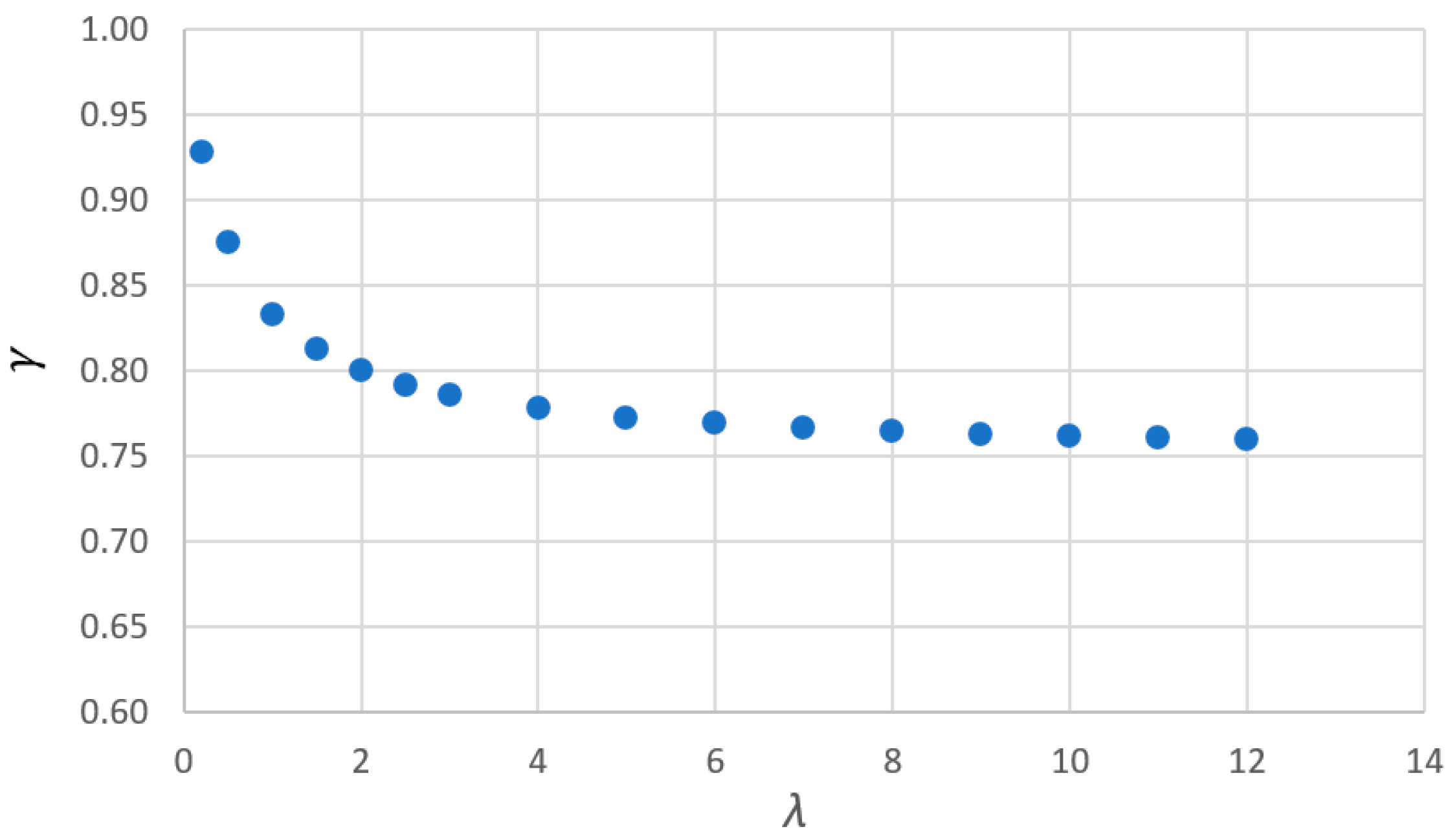Mualem [28] reported that typical values for $\lambda$ in Equation (41) range from 0.2 to 12 for different types of soils. For the above given parameter values, the typical values for $\gamma$ vary in a relatively narrow range between 0.76 and 0.93 (Figure 3). 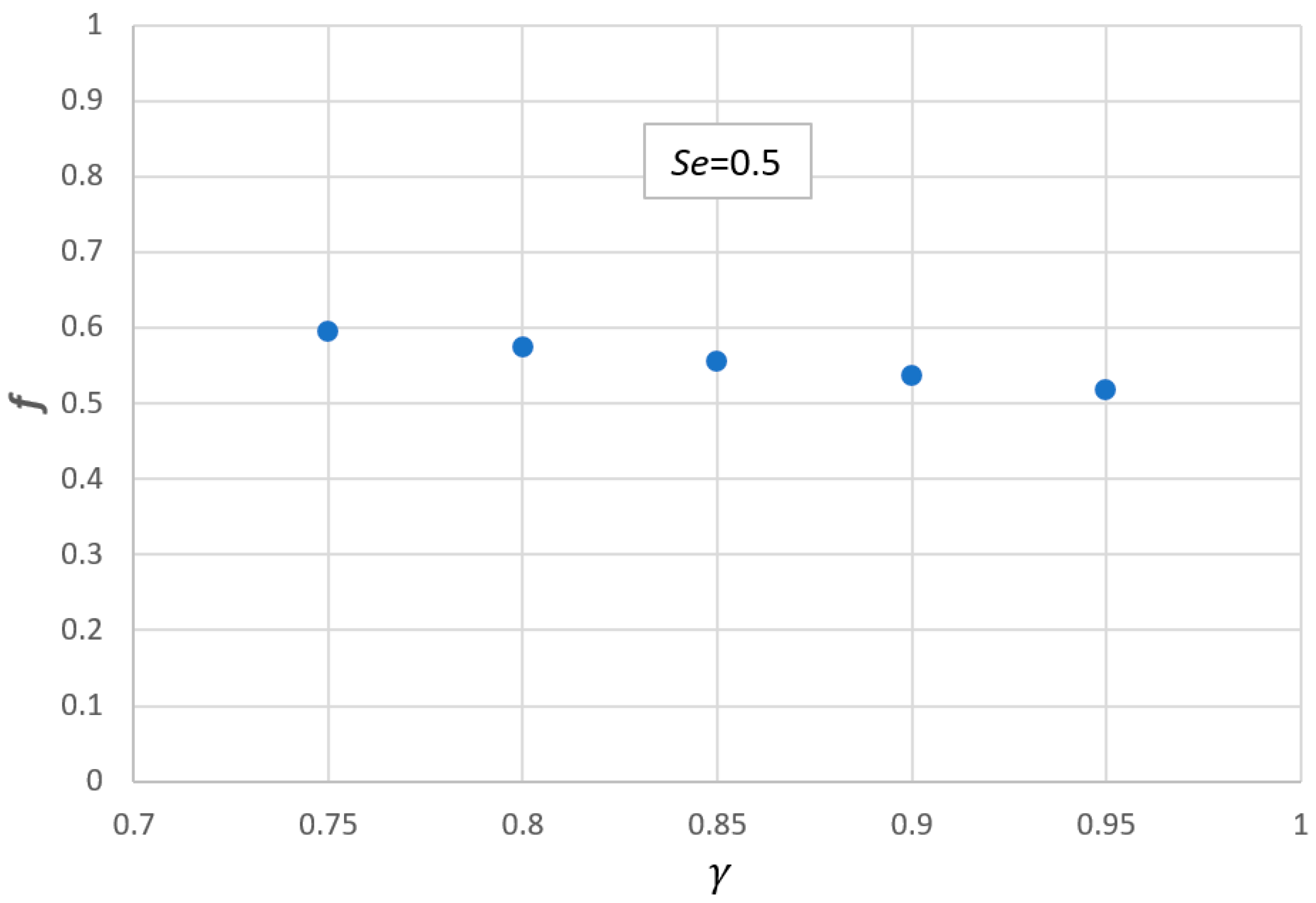For $\lambda$ > 2, $\gamma$ is between 0.76 and 0.80. Furthermore, Figure 4 shows that the fraction of the fingering flow zone f, the parameter that directly determines the large-scale fingering flow process, is not very sensitive to $\gamma$ when $\gamma$ takes its typical value between 0.76 and 0.93. Based on the above discussion, we can conclude that typical theoretical values for $\gamma$ are between 0.75 and 0.80 for most soils.

The theoretical values for $\gamma$ reported in this work are supported by previous experimental studies involving the determination of $\gamma$ values with field observations. Sheng et al. reported 13 dyed-water infiltration tests conducted in unsaturated soils at two different field sites, corresponding to loamy and clay soils, respectively, under various testing scales (or the sizes of infiltration plots) and total depths of infiltrated water [29]. For the clay-soil test site, the upper layer of soil was removed before the tests to eliminate the impact of observed macropores in the soil layer. For each test, dyed water was applied from the soil surface, which allowed for determination of water flow patterns by visualizing dye patterns. The patterns were mapped and water contents within the fingering flow were measured at different depths. Thus, from the measurements they could directly estimate the fractions of the fingering flow zone in horizontal planes at different depths and the average water content in the fingering flow zones at each depth. Consequently, they estimated $\gamma$ values for each test using Equation (36) that match the data reasonably well. Sheng et al. [29] observed that the estimated $\gamma$ values for two different soil types and a variety of test conditions were within a relatively narrow range between 0.62 and 0.79 with an average of 0.72. Liu et al. [30] also reported the $\gamma$ value estimated from the infiltration tests conducted by Öhrström et al. [31] was 0.80. Given the potential uncertainties involved in the data collection from the field-scale tests and the complexity of fingering flow patterns in the infiltration tests, the general consistency between theoretical and observed $\gamma$ values is remarkable.

3. Discussion

Darcy–Buckingham law was developed for water flow in unsaturated soil under the local-equilibrium condition. When preferential flow occurs, the local equilibrium does not hold any longer and alternative theoretical framework is needed for describing the water flow process. The preferential flow is mainly caused by the existence of macropores and wetting front instability (or fingering flow). Considerable attention has been given to the preferential flow associated with macropores [3,4], while water flow process in soils with macropores is similar to the process in unsaturated fractured rock, with macropores playing essentially the same role as fractures [5,6]. Although considerable laboratory studies and related theoretical investigations have been conducted for understanding and predicting properties of individual fingers and finger spacing, as reviewed by de Rooij [9], studies related to the development of macroscopic theory or modeling approaches for fingering flow are very limited. Unless computational technology is developed to such a level that we can routinely simulate large-scale fingering flow in unsaturated soils with a numerical grid-block size on the order of millimeter that allows for using the Darcy–Buckingham law to explicitly model individual fingers, a macroscopic theory for fingering flow is necessary for practical applications. At least for the foreseeable future, the fine-grid simulation mentioned above is not realistic.

This work provides a review of the on-going effort of developing a macroscopic theory for fingering flow. The theory does not seek to model individual fingers in detail, but to describe subgrid fingering in an average sense within the framework of the continuum approach that is convenient to use in practice. Since the local equilibrium assumption does not hold any longer, an alternative (optimality) principle was used for the theoretical development. The optimality principle states that water flows in unsaturated porous media in such a manner that the generated flow patterns correspond to the minimum global flow resistance. Unlike the Darcy–Buckingham law in which the conductivity is a function of capillary pressure or water saturation, the large-scale conductivity developed based on the optimality principle is also a power function of water flux, indicating that large hydraulic conductivities are allocated to locations where water fluxes are large to minimize the global flow resistance. As a parallel effort, a large-scale conductivity relationship was also derived by considering the fractal nature of fingering flow. This is mainly a descriptive, rather than physics-based method. Nevertheless, we demonstrate that the results from the two methods are essentially identical at least in an approximate sense. We also found that the theoretical values for the key parameter $\gamma$ in our model vary in a relatively narrow range between 0.75 and 0.80 for most soils, which is supported by the observations from previous field tests. As previously indicated, given the potential uncertainties involved in the data collection from the field-scale tests and the complexity of fingering flow patterns in the infiltration tests, the general consistency between theoretical and observed $\gamma$ values is remarkable. This finding also makes it easy to apply the new theory to field sites where experimental data are not readily available for estimating the $\gamma$ value.

The current models for describing water flow in macropores assume that the water flow is uniform in the macropore medium [3,4]. However, because water flow in these pores is gravity dominated, fingering flow could also occur in the pore network when the density of macropores is high enough that they can form a continuum. The evidence to support this point of view is available from the studies on water flow in unsaturated fractured rocks if we can use fractures as an analogue of macropores. Liu et al. reported that in the densely fractured unsaturated zone of Yucca Mountain, Nevada, only less than 10% of connected fractures had conducted water flow based on the analysis of the fracture coating data while other fractures were simply by-passed because of fingering flow in the fracture network [6]. Thus, Liu et al. argued that the macroscopic conductivity model developed herein for fingering flow should also be applicable to modeling water flow in macropores [31].

The implementation of our theory and related relationships into an existing numerical simulator is relatively straightforward and only involves modifying certain constitutive relations. The capillary pressure is a function of water saturation in fingering flow zone, rather than average saturation of a numerical grid-block. The former saturation is the ratio of the latter to the fraction of the fingering flow zone f. The mathematical expression for the relationship between capillary pressure and water saturation in the fingering flow zone is the same as the widely used local-scale expressions [12,13]. The fraction of the fingering flow zone f can be determined using Equation (36) with a $\gamma$ value between 0.75 and 0.80 for most soils. The unsaturated hydraulic conductivity is the local-scale conductivity as a function of water saturation within the fingering flow zone [12,13] multiplied by the fraction of fingering flow zone f. Further details of the implementation of our theory are available in Liu et al. [6,30] and Engstrom and Liu [32].

Finally, it is useful to comment on the potential limitations of the current theory. During the discussions in this and previous sections, initial water saturation has been assumed to be the residual water saturation. This is not the case for most field-scale problems of water flow in unsaturated soils. While an approximate approach to dealing with this issue (that assumes initial water saturation in the nonfingering flow zone to be immobile) was given in Liu et al. [30], a more rigorous approach needs to be developed in the future. When initial water saturation is higher than the residual saturation, two flow regimes coexist. The nonfingering flow zone corresponds to a relatively uniform and slow flow process that can be described by the conventional Darcy–Buckingham law. The flow process within the fingering flow zone needs to be described by the current theory. A more rigorous approach should be able to consider the coexistence of the two flow regimes, including their interactions on the subgrid scale.

One feature of gravitational fingers in porous media that receives considerable attention is the so-called saturation overshoot [33,34,35]. The overshoot is the pile-up of water at the fingering front where the water saturation near the front is higher than that within the finger body above the front. Our current theoretical framework focuses on the fully developed fingering flow process, as previously indicated, and thus is more suitable for capturing fingering flow behavior and average properties above the wetting front and is not able to capture the saturation overshoot near the wetting front. If the saturation overshoot becomes important for some practical applications, our theory needs to be refined to incorporate the overshoot phenomena on a large scale.

4. Concluding Remarks

This paper reviews a recent effort in developing a macroscopic theory to describe gravitational fingering flow of water in homogeneous and unsaturated soils, based on the optimality principle that water flows in unsaturated soils in such a manner that the generated flow patterns correspond to the minimum global flow resistance. The key difference between the new theory and the conventional unsaturated flow theories is that the unsaturated hydraulic conductivity in the new theory is not only related to water saturation or capillary pressure, but also proportional to a power function of water flux. This is because the water flux is closely related to the fingering flow patterns that allow for the existence of large hydraulic conductivity at locations where water fluxes are large to minimize the global flow resistance. The resultant relationship for the fraction of fingering flow zone is compared with that obtained from a parallel effort based on the fractal nature of the fingering flow pattern. The relationships from the two efforts are found to be essentially identical for gravity-dominated water flow in unsaturated soils and can both be expressed as a power function of the water saturation. This work also demonstrates that the theoretical values for the exponent of the power function vary in a relatively narrow range between 0.75 and 0.80 for most soils, which is supported by observations from previous field tests. This remarkable consistency makes it easy to apply our theory to field sites where experimental data are not readily available for estimating the exponent value.