Article

Assessing Streambed Stability Using D50-Based Stream Power Across Contiguous U.S.

1
Department of Civil, Architectural, and Environmental Engineering, North Carolina A&T State University, Greensboro, NC 27410, USA
2
Department of Geoscience, Baylor University, Waco, TX 76798, USA
3
Grassland Soil and Water Research Laboratory, USDA-ARS, Temple, TX 76502, USA
*
Author to whom correspondence should be addressed.
Water 2022, 14(22), 3646; https://doi.org/10.3390/w14223646
Submission received: 26 September 2022 / Revised: 8 November 2022 / Accepted: 10 November 2022 / Published: 12 November 2022
(This article belongs to the Section Water Erosion and Sediment Transport)

Abstract

:
Streambed aggradation and degradation are ways in which a stream will respond to changes in the incoming flow and sediment loads. Several environmental and societal problems are attributed to these channel bed adjustments. Prior studies have extensively used stream power to discern dominant channel processes and establish threshold limits required to trigger channel modifications. However, these studies were constrained by limited datasets and the scope of the applications. The current study used a large dataset of streambed median grain size (D50) across the contiguous U.S. in conjunction with a screening tool to assess the streambed stability for channel erosion and deposition potential. Analysis at the Physiographic Province level indicated major geomorphic changes are highly likely to occur in the Blue Ridge and Pacific Border provinces. Deposition-dominated streams are prominent in the Central Lowland, Great Plains, and Coastal Plain, whereas the Colorado Plateaus and Wyoming Basin have the highest percentage of stable channels. Smoothed spatial maps of stream power indicated the prevalence of high stream power in the Northeast and Pacific Northwest regions of the U.S. Comparison of channel erosion and deposition predictions using the stream power map with actual field calculated aggradation and degradation results yielded a 55% prediction accuracy. Further analysis based on the stream order revealed the association of higher stream power with lower stream orders.

1. Introduction

A thorough understanding of the balance between channel aggradation and degradation potential is essential for effective river management. Many environmental and societal predicaments including structural failures, habitat losses, and water quality deteriorations can be attributed to stream instability [1,2,3]. Channel aggradation or degradation are ways in which a stream will respond to changes in the incoming water flow and sediment load. Geomorphological and hydrological alterations that can arise from anthropogenic and natural events are the two major factors that induce stream instability [4]. The severity of these responses is contingent upon the landscape characteristics and geoclimatic factors [2]. Channel responses usually occur in the form of channel widening or narrowing, downstream aggradation, and upstream degradation [5]. Anticipation of the potential channel response can provide managers with time to design an efficient and well-suited stream rehabilitation scheme [6].
Channel instability in the past has been correlated with dominant geomorphic processes that unfold within a stream channel. Brice [7] correlated the instability of stream channels with the significance of the rate at which changes such as lateral bank erosion, streambed aggradation/degradation, and fluctuation of streambed elevation occur in a river. Spatial and temporal trends of these channel changes are usually illustrated using indicators that describe the characteristics and conditions of the channel [8]. Sediment transport formulas that use variables such as critical shear stress, bankfull discharge, median grain size, and channel slope have been used extensively to assess stream channel stability [9,10]. However, complex flow and sediment transport conditions cannot be adequately portrayed using such data-intensive conceptual frameworks [11]. Accordingly, recent studies have explored the usage of parameters requiring fewer resources such as stream power to examine channel morphological adjustments and sediment transport [11,12,13,14]. The ease involved in its computation and the proliferation of the digital elevation model (DEM) that allows the estimation of channel slope with higher precision have made stream power an ideal stream assessment tool [6,15].
Stream power is a vital metric that drives stream and floodplain-attributed processes including sediment transport and deposition [16]. Many aspects of the fluvial system have been shown to be impacted by stream power [17]; hence, it has been used as a practical means of investigating channel geomorphic processes. When compared with shear stress, critical specific stream power was found to be more viable in depicting sediment transport [14,18]. This justifies its extensive usage in sediment transport and channel characterization studies. The applicability of stream power as a predictor of channel modifications was investigated by Yochum et al. [19]. They used peak unit stream power values to establish different classes of geomorphic changes that unfolded in confined and unconfined stream channels. The total and specific stream power computed at and upstream of a location was used by Bizzi and Lerner [13] to identify the susceptibility of channels to erosion or deposition dominance. Cao et al. [20] used stream power to successfully quantify sediment transport rates both in ephemeral and perennial rivers when incorporating physically sensible parameters such as sediment particle size. Nanson and Croke [21] used the relationship between stream power and sediment character to classify floodplains. Several studies, on the other hand, tried to establish stream power threshold values to predict stability conditions and channel patterns [15,22,23,24]. Despite its importance, the number of studies that have investigated the applicability of stream power as a stream stability assessment tool on a broad spatial scale is still lacking.
The use of stream power as a preliminary screening tool to predict the susceptibility of a river to erode or deposit following interventions has gained interest in recent studies [25]. The Stream Power Screening Tool is an initial decision-making tool that foretells the likelihood of erosion and deposition within river channels. It is a graphical presentation of the power that resides in a stream. Brookes [23] applied the screening tool to channelized rivers in Denmark and developed power threshold values that corresponded with distinct channel processes. It has also been applied as a reconnaissance tool to anticipate the likely occurrence of adverse geomorphological adjustments in rivers of the UK [25]. Stacey and Rutherfurd [26] applied the screening tool while investigating the stability of sites in Virginia, although they were not able to discriminate between stable and unstable sites. Most studies that dealt with stream power-based investigation of channel stability were conducted on a smaller scale. Moreover, the limited number of data used in these studies confines their applicability scope and hampers their adaptability to large-scale investigations. Furthermore, previous applications of the tool disregarded the role of bed and bank material composition on the stability of a channel, keys to the assessment of bed stability.
This study aims to assess the use of stream power as a potential predictor of channel stability conditions (degradation and aggradation potential) using a comprehensive database of median grain size (D50) of streambed from across the contiguous U.S. A screening tool with embedded power threshold values was applied at the Physiographic Province level to examine streambed stability. Spatial maps that portray stream power and dominant channel process distributions were also prepared. The results of this study can be of use for future hydrologic and river management studies in terms of providing a general perspective into channel conditions of streams located within the U.S.

2. Materials and Methods

2.1. Stream Power

The concept of stream power was introduced by Bagnold [27] and since has been extensively used to characterize channel processes in both alluvial and gravel-dominated streams. Bagnold [27] developed an equation for the stream power needed to initiate the movement of grain particles, as follows:
Ω = ρ g Q S
where Ω is the unit-length stream power (W/m), ρ is water density (kg/m3), g is the gravitational acceleration (m/s2), Q is discharge (m3/s), and S is the channel slope. The equation is further modified for stream power per unit bed area of a stream reach (Bagnold [27]):
ω = Ω W = ρ   g   Q   S W
where ω is stream power (W/m2) and w is channel width (m). This equation indicates that the stream power is a function of slope, width, and discharge, which are easily extractable parameters. Similarly, in relatively recent study by Parker et al. [14], discussed further by Camenen [28] and Ferguson [29], they proposed a simplified equation for stream power (ω) which solely bases on the median grain size (D50), as follows:
ω = 0 . 1   ρ   [ ( SG   -   1 )   g   D 50 ) ] 3 / 2
where SG is the sediment specific gravity (~2.65).
This study used Equation (2) as “available” stream power, and Equation (3) as “critical” stream power in the analysis of degradation and aggradation processes in river channels.

2.2. Sources of D50 and Hydrological Data

A D50 dataset containing 2453 data points across the contiguous U.S. from five different sources was used in this study. A detailed description of the data variables, data sources, and data preparation can be found in Jha et al. [30]. Table 1 provides information on the number of data points, from each of the sources, for which D50 and other data were available including bankfull discharge (Q), width (W), depth (D), channel slope (S), and drainage area (DA). Additionally, the National Hydrography Dataset (NHD+) was used to acquire the data on W, D, and S at corresponding points with available D50 data [31]. The NHD+ data provides an accurate characterization of the river network through a high volume of attribute data depicting the hydrologic relations between stream segments and their interaction with surrounding catchments [32]. Furthermore, slope data were extracted at designated D50 points from the Soil Survey Geographic Database (SSURGO), State Soil Geographic Dataset (STATSGO) spatial data for comparison purposes.

2.3. Scale of Analysis

Regional frameworks for data analysis and interpretation are beneficial because they can give an insight into the correlation between spatial patterns and ecological and physical variables at the landscape scale [37]. The Physiographic Provinces of the contiguous U.S. developed by Fenneman and Johnson [38] were used in this study as a conceptual framework to regionalize the data analysis. They classified the contiguous U.S. into eight divisions and twenty-five provinces based on the topographical layout and geological conditions. Some of the previous applications of this framework for regional analysis include Bieger et al. [35] and Blackburn-Lynch et al. [39], which used Physiographic Divisions for developing bankfull hydraulic geometry relations, and Johnson and Fecko [40], which used these boundaries for establishing channel geometry equations. Figure 1 shows the distribution of D50 data points used in this study over Physiographic Provinces across the contiguous U.S. The Central Lowland province contained the highest number with 241 data points, whereas the St. Lawrence Valley province received the lowest with only 3 data points. Details on the number of data points and other associated hydraulic parameter information are provided in Table 2 under the results and discussion section.

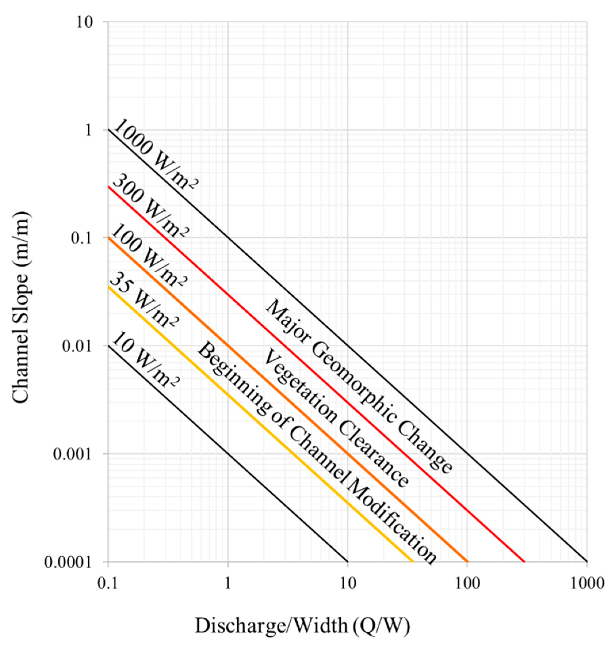
2.4. Stream Power Screening Tool

The stream power screening tool is a rapid means of assessing channel conditions through readily available hydrological variables. It graphically presents the stream power available at a river as the product of the bankfull discharge per unit width and the channel slope. The screening tool incorporates a series of lines that represent threshold stream power values: 10 W/m2, 35 W/m2, 100 W/m2, 300 W/m2, and 1000 W/m2 from bottom to top respectively (Figure 2). Previous applications of the screening tool revolved around predicting channel likelihood to erode or deposit after an intervention [23,41,42,43]. Despite the simplicity involved in its computation, threshold stream power values that correspond with geomorphic adjustments have not been defined clearly. In a study of channelized low-gradient rivers located in the UK and Denmark, Brookes [23] proposed a stream power threshold of 35 W/m2 to identify between stable and unstable rivers. Bizzi and Lerner [13] studied two sinuous single-thread channels with a bed majorly composed of boulder, cobble, and gravel, and suggested a stream power threshold of 34 W/m2 to classify erosion-dominated and stable channels. In a study conducted on a river basin located in Mississippi with a median bed size ranging from 0.2 to 0.5 mm, Bledsoe et al. [22] concluded that streams will attain a state of stability when the stream power is lower than 30 W/m2. Despite the comparability between the threshold values for stability presented in these studies, field investigations have shown contrasting values. Zavadil et al. [44], using field data collected from rivers in Australia, showed that stable incised streams can exhibit a stream power as high as 60 W/m2. A low-gradient river with an unconsolidated fine-grained bed in Illinois, on the other hand, starts to meander at a stream power of 10 to 20 W/m2 [16].
Similar discrepancies are witnessed in the threshold value that corresponds with the initiation of major geomorphic changes. Miller [24] studied stream power trends in Central Appalachian Mountains and observed the occurrence of severe damage on the stream bed when the stream power exceeds 300 W/m2. Indicating the successful application of the 300 W/m2 threshold in areas with different climatic and geomorphic conditions to discern channel responses, Buraas et al. [45] emphasized the universality of this threshold. Nevertheless, extreme flood events investigated in different studies elucidated that this threshold can be exceeded with no major geomorphological changes. For example, Yochum et al. [19] showed that their study sites underwent nominal geomorphological changes despite experiencing a stream power within the range of 800 to 1000 W/m2. This variability reveals that floods of similar magnitude can have wide-ranging impacts based on particle size distribution, cross-section characteristics, channel confinement, and channel alignment [16].
Even though the exceedance of the 300 W/m2 threshold cannot assure geomorphic instability, it can be tied to the initiation of major geomorphic changes [19]. Furthermore, the stream power thresholds for the initiation of channel erosion as proposed in the work of [13,22,23] all fell within the range of 30 to 35 W/m2 despite the former being conducted on a coarse-bedded channel whereas the latter two on a fine bedded channel.
This study used the screening tool in conjunction with threshold values to quantify the potential channel morphological changes under prevailing conditions and examine the variations in stream power amongst Physiographic Provinces. A threshold of 300 W/m2 was adopted to identify channels prone to major geomorphic change and a threshold range of 30 to 35 W/m2 was set to identify channels susceptible to erosion. Moreover, a threshold range of 15 to 25 W/m2 was adopted from Brookes [23]. The use of a screening tool requires three input parameters: channel slope (S), bankfull discharge (Q), and bankfull width (W). Channel slope and bankfull discharge were not available at all D50 data points, so further investigation was conducted to complete the dataset for use in the screening tool.

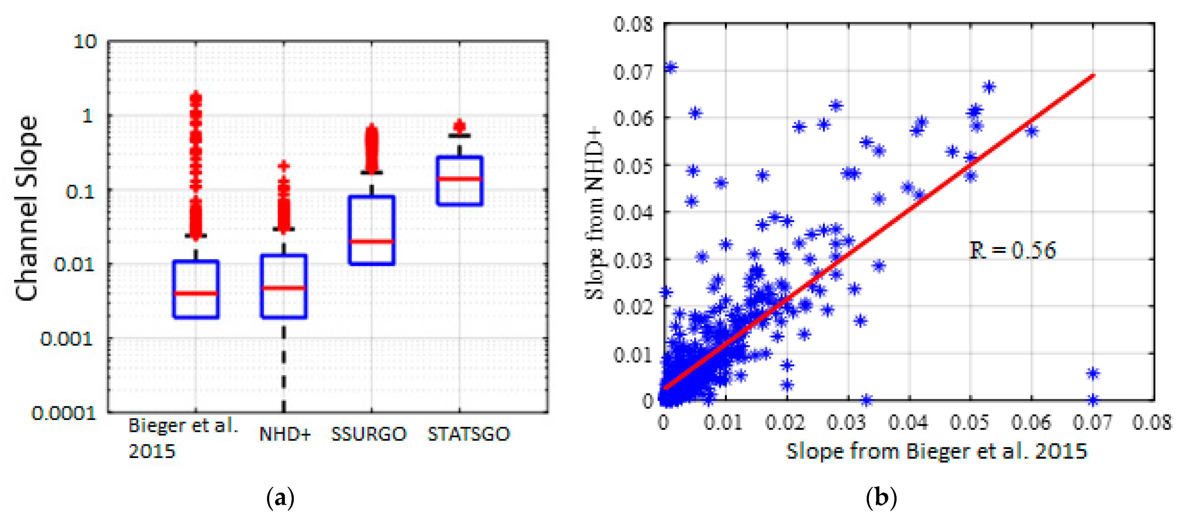
2.5. Slope at D50 Data Points

The slope data is very important as it can significantly influence the position of data points on the screening tool. Using the latitude and longitude of D50 data points, slope data were extracted from Soil Survey Geographic Database (SSURGO), State Soil Geographic Dataset (STATSGO), and NHD+. These data were compared with the slope data reported in Bieger et al. [33], which provided the slope data for most of its data points. Figure 3a shows the box plot of channel slope data for 560 data points from all four sources. STATSGO was found to clearly overpredict the slope data significantly. For SSURGO, in addition to overprediction, it did not return a corresponding slope value for 60 percent of the data points due to missing data in the original SSURRGO database. Consequently, because of its proximity to the data reported in the publication and its comprehensiveness, NHD+ was selected as a credible source of the slope data. A magnified scatter plot of slope values (slope < 0.08) from NHD+ and Bieger et al. [33] is presented in Figure 3b, which shows a moderate correlation (R2 = 0.56) between the two data sets.

2.6. Bankfull Discharge at D50 Data Points

The bankfull discharge, as defined by Simon et al. [46], is a channel-forming flow that has a considerable geomorphic significance. Stream power computation is commonly done for the bankfull discharge, which is usually taken to be a flow with a 1.5-year recurrence interval [12] or a 2-year recurrence interval [13]. The bankfull discharge data are usually not readily available but are generally developed using regional regression equations. Simon et al. [46] established a bankfull discharge relationship with the corresponding drainage area for 76 Level III Ecoregions. Likewise, Liu [47] presented an empirical power relation between the bankfull discharge and drainage area for 19 HUC2 water resource regions. The quasi-universal relation proposed by Parker et al. [48] described bankfull hydrologic geometry parameters, including bankfull discharge, using dimensionless equations. They used the bankfull discharge as a regressor to describe the bankfull depth, bankfull width, and slope. Due to the more refined spatial level of analysis, the regression relations developed by Simon et al. [46] were selected as a primary method to develop the bankfull discharge data used in this study. However, the accuracy of the predictions is examined using the equations and methods presented by Liu [47] and Parker et al. [48].
The bankfull discharge was computed for 1829 data points out of the total 2208 data points. The remaining points were in ecoregions whose regression coefficients and exponents were not provided in the publications. A t-statistics hypothesis test with a confidence level of 95% was conducted between the means of discharge estimates from Liu [47] and Simon et al. [46] relations to evaluate their correspondence. The null hypothesis that claimed similarity between the two means was supported by a test statistic of 0.517 and a p-value of 0.302, which were lower and higher than the critical value (1.96) and the level of significance (0.05) respectively. Secondary verification of estimated discharges by Simon et al. [46] was conducted using the quasi-universal relations of Parker et al. [48]. Data on bankfull width, bankfull depth, and slope were adopted from the NHD+ database. For the comparative analysis, the bankfull discharge data estimated using Simon et al. [46] were transformed into their dimensionless version and plotted with the data points originally provided by Parker et al. [48] for the corresponding dimensionless width, depth, and slope. The dimensionless values (w’, h’, and Q’) were developed for each datapoints using the equations provided in Parker et al. [48]. Figure 4 shows the visual correspondence of these two data sources, revealing a good agreement, thus providing additional validation for using Simon et al. [46] regression equations to develop bankfull discharge data.

3. Results and Discussion

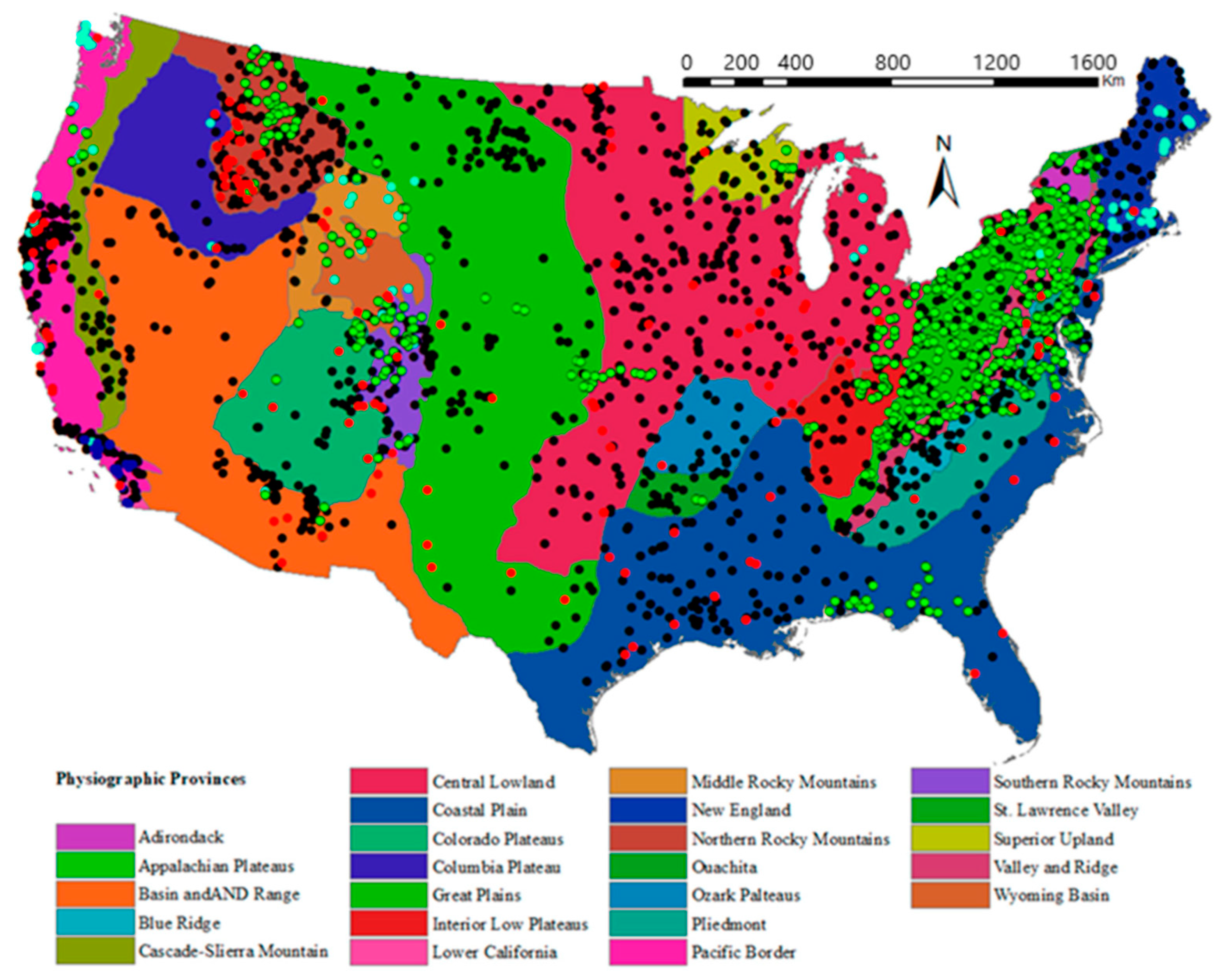
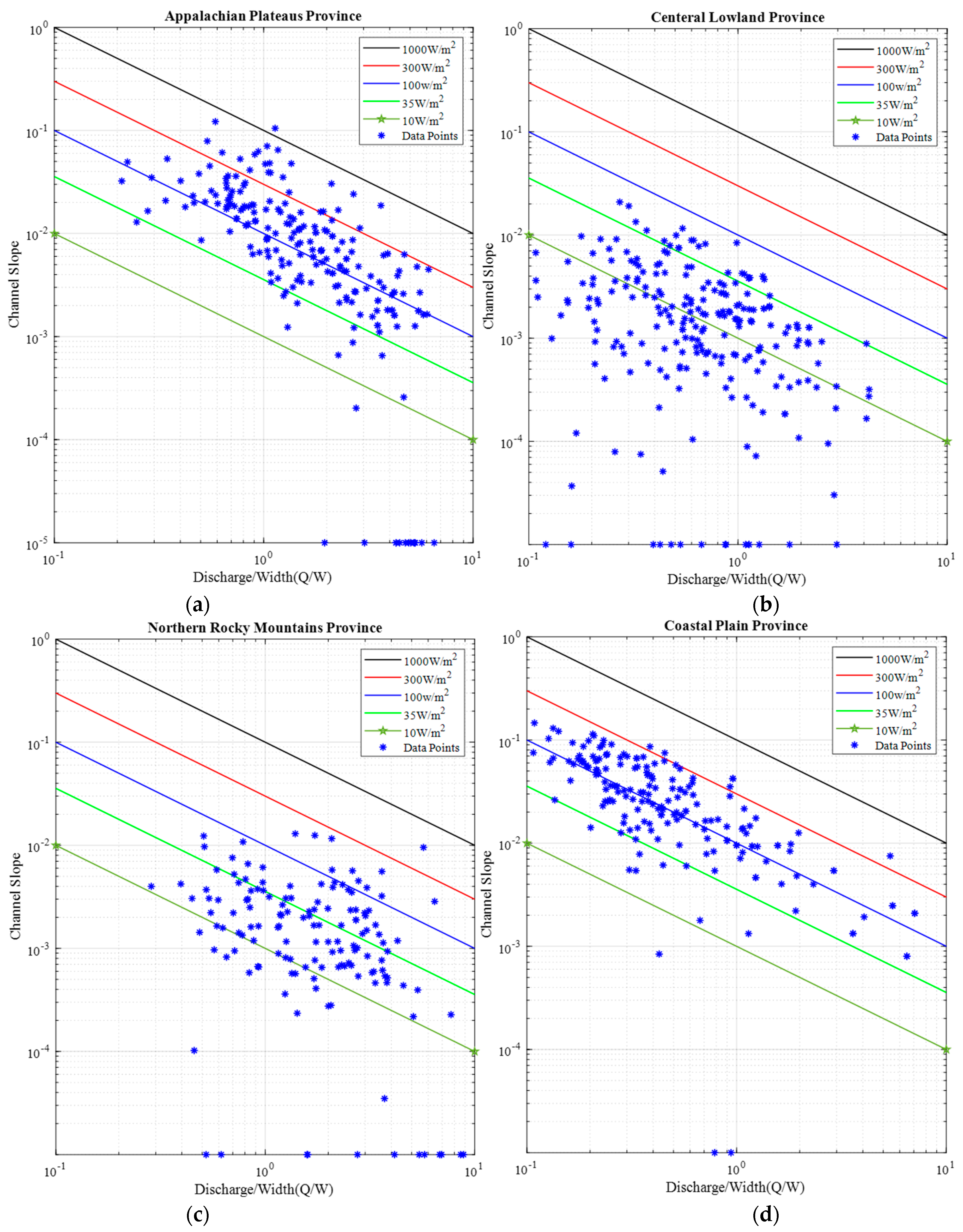
3.1. Stream Power Screening Tool by Physiographic Provinces

The screening tool was applied at the regional framework of the Physiographic Province level to analyze the aggradation/degradation potential based on the dataset developed for D50, channel slope, bankfull width, and bankfull discharge. Figure 5 shows the screening tool as being applied for four selected Physiographic Provinces that contained the highest number of data points: Appalachian Plateaus, Central Lowlands, Coastal Plains, and Northern Rocky Mountains. The positions of the data points with respect to the existing stream power lines indicate the potential power a stream possesses to perform morphological works.
The Appalachian Plateaus (Figure 5a) was found to be dominated by streams that have high power as compared to the remaining three regions. The stream power in this province ranged from 0.19 to 1169 W/m2. Ten percent of the data (23 points) were positioned above 300 W/m2, with the remaining majority laying within the range of 100 to 300 W/m2. Streams in this region are characterized by steeper slopes and narrower channels with bed material mainly composed of sand and gravel [8]. This is consistent with the range of channel slopes and widths compiled for this Physiographic region. The Central Lowland (Figure 5b), compared to the other three provinces, experienced a lower stream power that ranged from 0.023 to 261 W/m2 excluding outlying points, with a majority of the data points falling below the 10 W/m2 power line. The region has the highest width range accompanied by milder slopes and high bankfull discharges. Similarly, the Northern Rocky Mountain province (Figure 5c), the course grain bedded and steep-sloped mountainous streams [8], possessed streams with power ranging from 0.08 to 700 W/m2. Streams in the Coastal Plain province (Figure 5d) exhibited a stream power that ranged from 0.05 W/m2 to 533.33 W/m2. For this region, characterized by gently sloped streams [8,49], more than 90 percent of the data points fell below the 300 W/m2 stream power threshold line despite large discharge ranges. This agrees with MacBroom et al. [16], who pointed out the decrement possibility of stream power in areas with higher discharge but with a decreasing slope downstream.
Table 2 provides comprehensive information by Physiographic Provinces for physical attributes of streams, stream power ranges, and the percentage of data points that lie below or above the threshold values. This information is useful in generally assessing the likelihood of aggradation and degradation potential of streams in different provinces. Specifically, the Blue Ridge and Pacific Border provinces have streams that are highly prone to major geomorphological adjustments with more than 50 percent of the study sites located in each of these regions experiencing a stream power higher than 300 W/m2. The deposition was seen to be a dominant process in the Central Lowland, Great Plains, and Coastal Plain provinces with a considerable number of data points having stream power lower than 15 W/m2. Johnson [8] also asserted the tendency of streams within the Great Plains to serve as a depositional environment for sediment derived from the mountainous west. The Colorado Plateaus and Wyoming Basin, whose stream channels are composed of bedrock or semi-alluvial and large bank and bed material respectively [8], saw the highest percentage of data points that had a stream power which allows channel stability. Overall, the majority of the Physiographic Provinces contained data points with stream power higher than 35 W/m2. This indicates the susceptibility of most of the stream sites assessed in this study to channel erosion. It should be noted that these results are subjective to the locations of data points and also the quantity of the data that explains it.

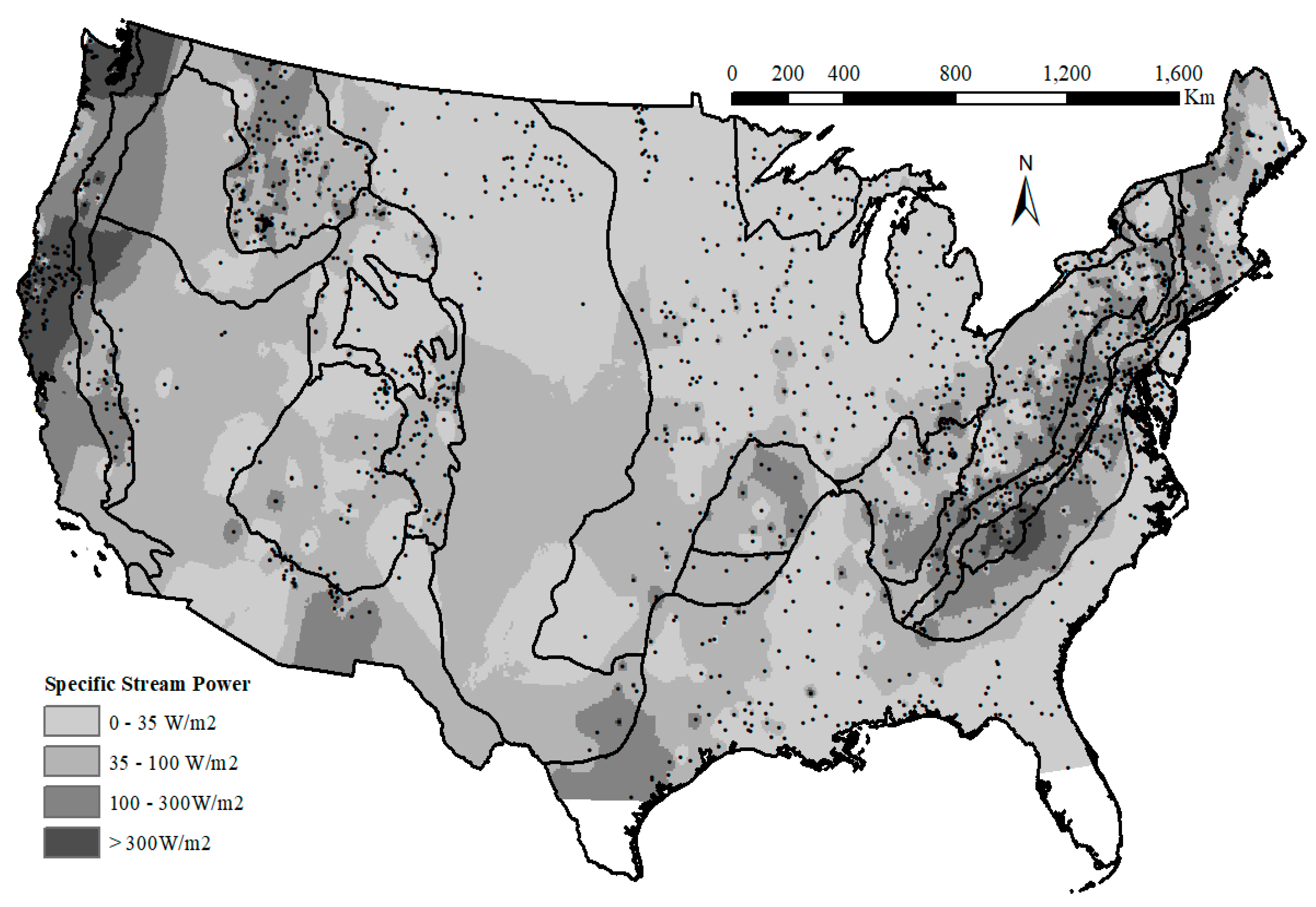
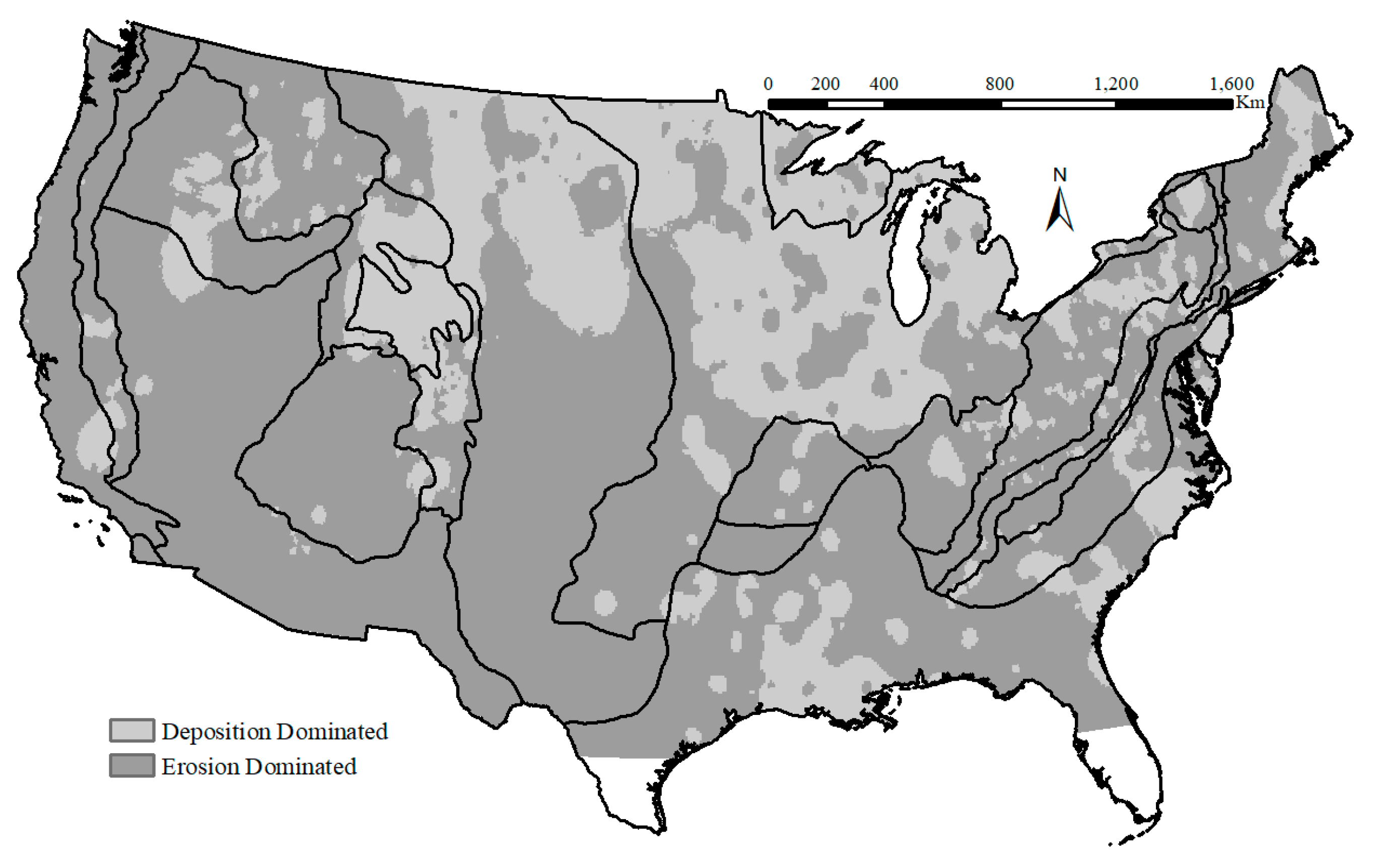
3.2. Interpolation of Stream Power across Contiguous U.S.

Stream power at each data point was calculated using Bagnold’s equation (Equation (1) to develop a series of spatial maps showing the distribution of “available stream power” across the contiguous U.S. Figure 6 depicts an interpolated map prepared based on a function in ArcMap that uses the technique of inverse distance weighted interpolation. In this method, the weighted averages of nearby observations are calculated to assign raster cell values; the weight depends on the distance between the observation and the raster cell. Since the stream power values exhibit broad spatial variation from inconsistency in geological condition, particle size distribution, channel alignment, and channel cross-section characteristics, the logarithmic values of stream powers were used in map development to ameliorate the effect of large spatial variation. The logarithmic values were then converted back to “W/m2” in legend for easier interpretation and visualization. Four classes of stream power were mapped across the contiguous U.S. The two higher-stream power classes mainly dominated the Pacific Northwest and Northeast regions, whereas the Midwest, Southeast, and Southwest regions were majorly dominated by the two lower-stream power classes.
Likewise, a spatial map of “critical stream power”, that defines the amount of stream power needed to initiate the movement of a grain particle, was developed using Equation (3). The difference between the “critical stream power” and “available stream power” was then used to classify erosion- and deposition-dominated streams. Channels with higher available stream power were classified as erosion-susceptible channels, whereas those with higher critical stream power were labeled as deposition-dominated channels. This assumption did not consider the existing sediment concentration of the river which, in combination with the sediment transport capacity, will drive the actual erosion or deposition. The magnitude of the stream power higher/lower than that of the critical threshold only indicates the higher/lower sediment transport capacity.
Figure 7 presents the interpolated map showing areas with the corresponding degradation/aggradation channel processes. The logarithmic values were once again used for the map development process. As can be inferred from the map, much of the U.S. is classified as being predisposed to erosion. The Wyoming Basin, part of Grate Plain, and Central Lowland were among the provinces where deposition is seen to be dominant.

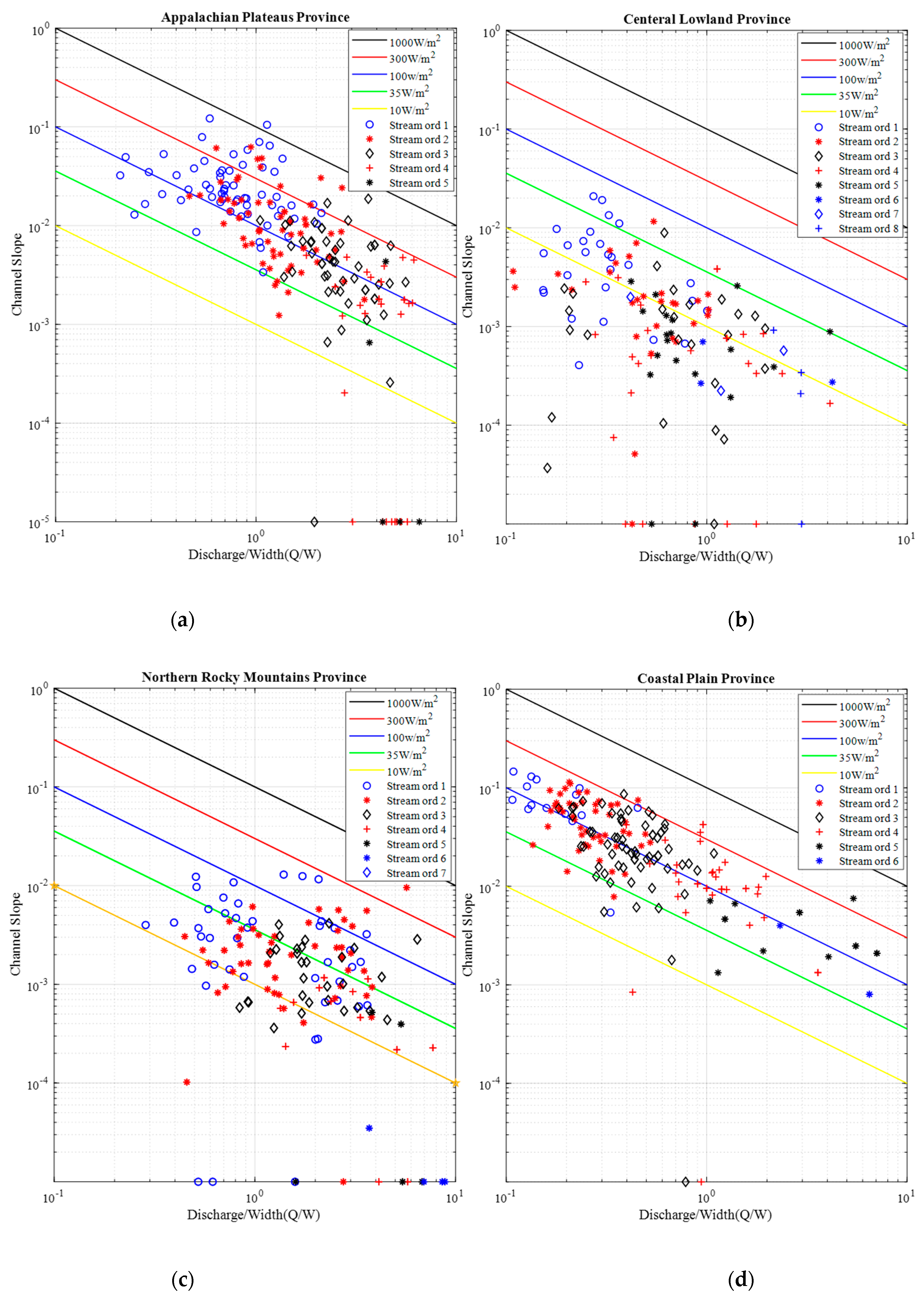
3.3. Analysis of Stream Power Based on the Stream Order

Streams adopt various channel forms as they flow from headwaters to their mouth that is guided by the interplay among variables including channel slope, discharge, and sediment type [50]. These channel variations can often be addressed using a stream order based classification. Stall and Fok [51] revealed a reasonable correlation between stream order, channel slope, and low frequency discharge. Similarly, [13,50] found prevailing channel gradients and discharge to govern the downstream patterns of change in stream power. Consequently, the variation in stream power and corresponding river forms and processes, which results from the combined effect of channel gradient and discharge, can thus be addressed using the concept of stream order.
For this stream order-based analysis of stream power, stream order data were extracted from NHD+ for all D50 data points. Using the latitude and longitude values, “COMID” a unique numerical identifier of stream segments within NHD+, was assigned to each data point. Hydrological and channel parameters were then extracted from the database based on their COMID. Figure 8 shows stream power data for four Physiographic Provinces on the screening tool based on stream order. It can be observed that most of the low order streams, characterized by steeper slopes, low discharge, and narrower channels, are placed on the top left corner of the screening tool showing a higher stream power. Conversely, the higher order streams characterized by low gradient, high discharge, and wider channels were placed on the bottom right side of the screening tool.
Sorting the data points by stream order basis, as provided in Table 3, indicated both channel slope and bankfull discharge adopt a decremental and incremental pattern respectively, with a corresponding increase in stream order. Likewise, the range of stream power was seen to decrease with an increase in stream power. Channel processes operating within a river system were highly correlated with the downstream change in stream power. Major geomorphological changes and channel erosions were prevalent in low order streams, with much of the data points exhibiting stream power exceeding 35 W/m2. The higher order stream (6 and 7) were majorly prone to deposition, with more than 50 percent of their data points attaining a stream power lower than 15 W/m2. Although the general decremental pattern of stream power with an increase in stream order was maintained in most cases, high stream power values were also found in higher order streams.

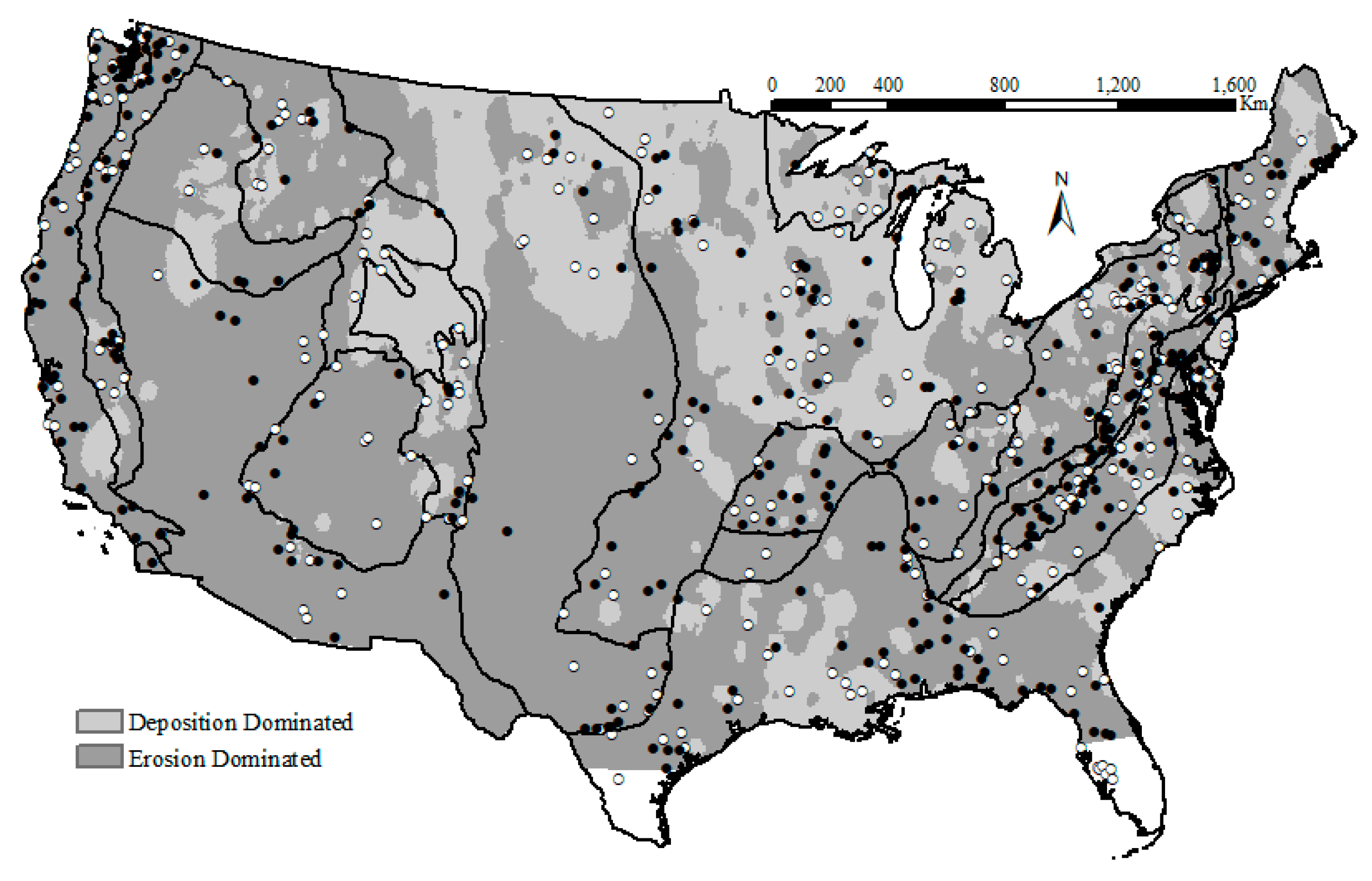
3.4. Comparison with Long-Term Erosion/Deposition Temporal Data

An analysis was attempted to assess the reliability of the erosion/deposition pattern. Figure 7 was compared with long-term temporal data provided by Slater and Singer [36], which provided the decadal trends of riverbed aggradation and degradation on 623 USGS gaging stations over a period of 61 years (1950–2011). Using the longitudinal and latitudinal location of these gaging stations, we overlaid these points of aggradation/degradation on the spatial map of erosion/deposition developed in Figure 7. The comparison resulted in the agreement of 55% (332) of the data points, as can be seen in Figure 9, for which erosion points matched with the degradation area and deposition points matched with the aggradation area. A few points did not get compared as they fell over areas with no raster values (white regions) on the interpolated map. It should be noted that the comparative analysis presented here used a spatial map (developed using about 2000 data points across the contiguous U.S.) overlaid with 623 observation points (not uniformly distributed across the area). In addition, these are very small datasets compared to the vast geographic area we selected for the analysis. With these uncertainties at hand, agreeing with more than half of the observation data points is remarkable.

4. Conclusions

This study used an extensive dataset collected from five sources to evaluate stream channel conditions by applying a stream power-based screening tool. Stream power threshold values solely will not guarantee the occurrence of predicted channel processes; however, they can be linked with morphological adjustments. The study provided useful information in generally assessing the likelihood of aggradation and degradation potential of streams by Physiographic provinces. Major geomorphological changes are dominant in streams located in the Blue Ridge and Pacific Border provinces. Streams in the Central Lowland, Great Plains, and Coastal Plain provinces, compare to all other provinces, are prone to sediment deposition due to low stream power of less than 15 W/m2. We also developed an interpolated map that depicted stream power residing in different regions of the U.S. The Northeast and the Pacific Northwest are dominated by streams that possess higher erosive power, whereas streams in the Midwest, Southeast, and part of Southwest regions have a lower stream power. Analysis using the available and critical stream power, calculated at data points, and the resulting interpolated map delineated the regions depicting dominant channel processes including erosion and deposition. Further analysis based on stream order found that the low order streams that are characterized by steeper slopes, low discharge, and narrower channel width corresponded with higher stream power. Streams and rivers are dynamic systems and our effort to characterize their form and processes will continue to be constrained by data limitations. The data and analysis presented in this study are a starting point for a national scale stream power-based assessment of stream systems. The interpolation technique and hence accuracy of the smoothed maps are contingent upon the density of data points used. Some of the potential limitations of the analysis presented in this study are summarized below:
  • Stream power as a sole indicator for degradation/aggradation: This study relies on stream power to discretize the major geomorphological changes that could unfold in a stream channel. However, as noted by Bizzi and Lerner [13], stream power mainly accounts for the drivers of stream processes, slope, and discharge, with no characterization given to the resisting forces: sediments size distribution, bed lithology, and bedforms [12]. Yochum et al. [19] showed that variable stream power thresholds had been attributed to certain geomorphological changes in different studies, demonstrating the inadequacy of stream power to serve as a sole indicator of dominant channel processes. It is vital to understand and integrate both the driving and resisting forces while establishing threshold stream power values for actual channel condition prediction [16].
  • Threshold limits on the screening tool: Threshold values of stream power for stream conditions were developed and recommended based on limited datasets. These were intended to be used in an environment that resembles the original study sites [25]. Application of these threshold values in a broad spatial extent with different streambed substrate types, channel geometry, and geological conditions can lead to an obscured result. Nevertheless, this study adopted a range of threshold values to discriminate between channel types, intending to encapsulate minimum stream power values required for erosion instigation in both coarse- and fine-bedded stream channels. The effect of streambed grain size was also accounted for here through the computation of critical stream power. This enhances the channel discrimination competency conducted here compared to previous studies that disregard the effect of particle size distribution while establishing stream power thresholds.
  • Data limitation for large-scale application: The data used in this study was representative of the contiguous U.S. except for areas where spatial gaps were present. The data scarcity is majorly noticeable in the Great Plains, Basin and Range, and Colombia Plateaus provinces. Interpolation techniques used in the development of spatial maps highly depend on the density and distribution of data points. The accuracy of this map could have been improved if more data were available and added to the dataset. Nonetheless, the data presented in this study can serve as a foundation upon which a more comprehensive and representative analysis can be built.
Future studies can capitalize on the current database to establish a detailed and competent depiction of channel conditions across the contiguous U.S. Results from this study indicated stream power can reasonably estimate prevailing channel processes. However, factors including channel confinement, channel alignment, and cohesion, which could impact prevailing conditions, were not accounted for in this study. Additional research is needed on the influence of these variables to improvise prediction accuracy.

Author Contributions

Conceptualization, P.M.A.; Formal analysis, D.M.A.; Funding acquisition, M.J.W.; Investigation, M.K.J., P.M.A. and J.G.A.; Methodology, P.M.A. and J.G.A.; Project administration, M.K.J.; Resources, J.G.A. and M.J.W.; Software, M.J.W.; Supervision, M.K.J.; Writing—original draft, D.M.A.; Writing—review & editing, M.K.J. All authors have read and agreed to the published version of the manuscript.

Funding

This material is based upon work supported by the Agricultural Research Service (ARS), U.S. Department of Agriculture (USDA), under agreement number 58-3098-8-003. Any opinions, findings, conclusions, or recommendations expressed in this publication are those of the author(s) and do not necessarily reflect the view of the USDA. USDA is an equal opportunity provider and employer.

Institutional Review Board Statement

Not applicable.

Informed Consent Statement

Not applicable.

Data Availability Statement

Not applicable.

Conflicts of Interest

The authors declare no conflict of interest.

References

  1. Bledsoe, B.; Baker, D.; Nelson, P.; Rosburg, T.; Sholtes, J.; Stroth, T. Design Hydrology for Stream Restoration and Channel Stability at Stream Crossings; The National Academies of Sciences, Engineering, and Medicine: Fort Collins, CO, USA, 2016; Available online: http://onlinepubs.trb.org/onlinepubs/nchrp/nchrp_rpt_853_FinalReport.pdf (accessed on 1 October 2022).
  2. Kaufmann, P.R.; Larsen, D.P.; Faustini, J.M. Bed stability and sedimentation associated with human disturbances in Pacific Northwest streams. J. Amer. Wat. Res. Assoc. 2009, 45, 434–459. [Google Scholar] [CrossRef]
  3. Piégay, H.; Darby, S.E.; Mosselman, E.; Surian, N. A review of techniques available for delimiting the erodible river corridor: A sustainable approach to managing bank erosion. Riv. Res. App. 2005, 21, 773–789. [Google Scholar] [CrossRef]
  4. Lagasse, P.F.; Schall, J.D.; Johnson, F.; Richardson, E.V.; Chang, F. Stream Stability at Highway Structures; U.S. Department of Transportation, FHWA-IP-90-014; 1995. Available online: https://rosap.ntl.bts.gov/view/dot/25666 (accessed on 1 October 2022).
  5. Simon, A.; Downs, P.W. An interdisciplinary approach to evaluation of potential instability in alluvial channels. Geomorphology 1995, 12, 215–232. [Google Scholar] [CrossRef]
  6. Soar, P.J.; Wallerstein, N.P.; Thorne, C.R. Quantifying river channel stability at the basin scale. Water 2017, 9, 133. [Google Scholar] [CrossRef] [Green Version]
  7. Brice, J.C. Stream Channel Stability Assessment; Tech Report FHWA/RD-82/021; U.S. Geological Survey: Menlo Park, CA, USA, 1982. Available online: https://rosap.ntl.bts.gov/view/dot/34974 (accessed on 1 October 2022).
  8. Johnson, P.A. Assessing Stream Channel Stability at Bridges in Physiographic Regions; VirginiaFHWA-HRT-05-072; U.S. Department of Transportation: McLean, VA, USA, 2006.
  9. Olsen, D.; Whitaker, A.C.; Potts, D.F. Assessing stream channel stability thresholds using flow competence estimates at bankfull stage. J. Am. Water Resour. Assoc. 1997, 33, 1197–1207. [Google Scholar] [CrossRef]
  10. Rosgen, D.L. A Stream Channel Stability Assessment Methodology. In Proceedings of the Seventh Federal Interagency Sedimentation Conference, Reno, Nevada, 25–29 March 2001. [Google Scholar]
  11. Lea, D.M.; Legleiter, C.J. Mapping spatial patterns of stream power and channel change along a gravel-bed river in northern Yellowstone. Geomorphology 2016, 252, 66–79. [Google Scholar] [CrossRef]
  12. Petit, F.; Gob, F.; Houbrechts, G.; Assani, A.A. Critical specific stream power in gravel-bed rivers. Geomorphology 2005, 69, 92–101. [Google Scholar] [CrossRef]
  13. Bizzi, S.; Lerner, D.N. The use of stream power as an indicator of channel sensitivity to erosion and deposition processes. Riv. Res. App. 2015, 31, 16–27. [Google Scholar] [CrossRef]
  14. Parker, C.; Clifford, N.J.; Thorne, C.R. Understanding the influence of slope on the threshold of coarse grain motion: Revisiting critical stream power. Geomorphology 2011, 126, 51–65. [Google Scholar] [CrossRef]
  15. Ferencevic, M.V.; Ashmore, P. Creating and evaluating dem-based stream power maps as a stream assessment tool. Riv. Res. App. 2012, 28. [Google Scholar] [CrossRef]
  16. MacBroom, J.G.; Schiff, R.; Louisos, J. River and Stream Power Assessment Report Including Culvert and Bridge Vulnerability Analysis: Deerfield River Basin; Water Resources and Extension at ScholarWorks@UMass: Amherst, MA, USA, 2017; Available online: https://scholarworks.umass.edu/water_reports/4 (accessed on 1 October 2022).
  17. Knighton, A.D. Downstream variation in stream power. Geomorphology 1999, 29, 293–306. [Google Scholar] [CrossRef]
  18. Habersack, H.M.; Laronne, J.B. Evaluation and improvement of bed load discharge formulas based on Helley–Smith sampling in an Alpine Gravel Bed River. J. Hydrau. Eng. 2002, 128, 484–499. [Google Scholar] [CrossRef]
  19. Yochum, S.E.; Sholtes, J.S.; Scott, J.A.; Bledsoe, B.P. Stream power framework for predicting geomorphic change: The 2013 Colorado Front Range Flood. Geomorphology 2017, 292, 178–192. [Google Scholar] [CrossRef]
  20. Cao, Z.; Hu, P.; Pender, G. Reconciled bedload sediment transport rates in ephemeral and perennial rivers. Earth Surf. Proc. Landf. 2010, 35, 1655–1665. [Google Scholar] [CrossRef]
  21. Nanson, G.C.; Croke, J.C. A genetic classification of floodplains. Geomorphology 1992, 4, 459–486. [Google Scholar] [CrossRef] [Green Version]
  22. Bledsoe, B.; Watson, C.; Biedenharn, D. Quantification of incised channel evolution and equilibrium. J. Am. Water Resour. Assoc. 2002, 38, 861–870. [Google Scholar] [CrossRef]
  23. Brookes, A. The distribution and management of channelized streams in Denmark. Regul. Rivers Res. Manag. 1987, 1, 3–16. [Google Scholar] [CrossRef]
  24. Miller, A.J. Flood hydrology and geomorphic effectiveness in the central Appalachians. Earth Sur. Proc. Landf. 1990, 15, 119–134. [Google Scholar] [CrossRef]
  25. Wishart, D.; Brookes, A. Application of a Stream Power Screening Tool. In Accounting for Sediment in Rivers—A Tool Box of Sediment Transport and Transfer Analysis Methods and Models to Support Hydromophologically-Sustainable Flood Risk Management in the UK; Research Report UR9; Wallerstein, N.P., Ed.; Flood Risk Management Research Consortium: Watlington, UK, 2006; pp. 13–24. [Google Scholar]
  26. Stacey, M.; Rutherfurd, I. Testing Specific Stream Power Thresholds of Channel Stability with GIS. In Proceedings of the 5th Australian Stream Management Conference, Charles Sturt University, Thurgoona, Australia, 21–25 May 2007. [Google Scholar]
  27. Bagnold, R.A. An Approach to the Sediment Transport Problem From General Physics; Geological Survey Professional, Paper 422-1; United States Department of the Interior: Washington, DC, USA, 1966; Volume 422.
  28. Camenen, B. Discussion of “Understanding the influence of slope on the threshold of coarse grain motion: Revisiting critical stream power by C. Parker, N.J. Clifford, and C.R. Thorne Geomorphology, Volume 126, March 2011, Pages 51–65”. Geomorphology 2012, 139–140, 34–38. [Google Scholar] [CrossRef] [Green Version]
  29. Ferguson, R.I. River channel slope, flow resistance, and gravel entrainment thresholds. Wat. Resou. Res. 2012, 48, W05517. [Google Scholar] [CrossRef]
  30. Jha, M.K.; Asamen, D.M.; Allen, P.M.; Arnold, J.G.; White, M.J. Streambed Median Grain Size (D50) Across the Contiguous U.S. Water 2022, 14, 3378. [Google Scholar] [CrossRef]
  31. Huang, J.; Frimpong, E.A. Modifying the United States National Hydrography Dataset to improve data quality for ecological models. Ecol. Inform. 2016, 32, 7–11. [Google Scholar] [CrossRef]
  32. Hill, R.A.; Weber, M.H.; Leibowitz, S.G.; Olsen, A.R.; Thornbrugh, D.J. The Stream-Catchment (StreamCat) dataset: A database of watershed metrics for the conterminous United States. J. Amer. Wat. Res. Assoc. 2016, 52, 120–128. [Google Scholar] [CrossRef]
  33. Bieger, K.; Rathjens, H.; Allen, P.M.; Arnold, J.G. Development and evaluation of bankfull hydraulic geometry relationships for the Physiographic Regions of the United States. J. Amer. Wat. Res. Assoc. 2015, 51, 842–858. [Google Scholar] [CrossRef] [Green Version]
  34. USEPA. Wadeable Stream Assessment: A Collaborative Summary of the Nation’s Streams; (EPA) 841-B-06-002; United States Environmental Protection Agency: Washington, DC, USA, 2006. Available online: https://www.epa.gov/sites/production/files/2014-10/documents/2007_5_16_streamsurvey_wsa_assessment_may2007.pdf (accessed on 1 October 2022).
  35. Hawley, R.J.; Bledsoe, B.P. Channel enlargement in semiarid suburbanizing watersheds: A southern California case study. J. Hydrol. 2013, 496, 17–30. [Google Scholar] [CrossRef]
  36. Slater, L.J.; Singer, M.B. Imprint of climate and climate change in alluvial riverbeds: Continental United States, 1950–2011. Geology 2013, 41, 595. [Google Scholar] [CrossRef] [Green Version]
  37. McManamay, R.A.; Orth, D.J.; Dolloff, C.A.; Frimpong, E.A. Regional rrameworks applied to hydrology: Can landscape-based frameworks capture the hydrologic variability? Riv. Res. App. 2011, 28, 1325–1339. [Google Scholar] [CrossRef]
  38. Fenneman, N.M.; Johnson, D.W. Physiographic Divisions of the Conterminous U.S.; U.S. Geological Survey: Reston, VA, USA, 1946.
  39. Blackburn-Lynch, W.; Agouridis, C.T.; Barton, C.D. Development of regional curves for hydrologic landscape regions (HLR) in the Contiguous United States. J. Amer. Wat. Res. Assoc. 2017, 53, 903–928. [Google Scholar] [CrossRef]
  40. Johnson, P.A.; Fecko, B.J. Regional channel geometry equations: A statistical comparison for physiographic provinces in the eastern US. Riv. Res. App. 2008, 24, 823–834. [Google Scholar] [CrossRef]
  41. Brookes, A. Restoration and enhancement of engineered river channels: Some european experiences. Regul. Rivers: Res. Manag. 1990, 5, 45–56. [Google Scholar] [CrossRef]
  42. Nakamura, F.; Sudo, T.; Kameyama, S.; Jitsu, M. Influences of channelization on discharge of suspended sediment and wetland vegetation in Kushiro Marsh, Northern Japan. Geomorphology 1997, 18, 279–289. [Google Scholar] [CrossRef]
  43. Erskine, W.; White, L.J. Historical River Metamorphosis of the Cann River, East Gippsland, Victoria. In Proceedings of the First National Conference on Stream Management in Australia, Merrijig, Australia, 19–23 February 1996. [Google Scholar]
  44. Zavadil, E.; Hardie, R.; Blackham, D.; Ivezich, M. The Role of Stream Power and Strategic Native Vegetation Establishment in the Management of Incised River Stems. In Proceedings of the 7th Australian Stream Management Conference, Townsville, Queensland, 21–30 July 2014. [Google Scholar]
  45. Buraas, E.M.; Renshaw, C.E.; Magilligan, F.J.; Dade, W.B. Impact of reach geometry on stream channel sensitivity to extreme floods. Earth Surf. Process. Landf. 2014, 39, 1778–1789. [Google Scholar] [CrossRef]
  46. Simon, A.; Dickerson, W.; Heins, A. Suspended-sediment transport rates at the 1.5-year recurrence interval for ecoregions of the United States: Transport conditions at the bankfull and effective discharge? Geomorphology 2004, 58, 243–262. [Google Scholar] [CrossRef] [Green Version]
  47. Liu, Z. An Explicit Representation of River Networks in a Continental-Scale Catchment-Based Land Surface Model Framework. Ph.D. Dissertation, University of California, Berkeley, CA, USA, 2014. [Google Scholar]
  48. Parker, G.; Wilcock, P.R.; Paola, C.; Dietrich, W.E.; Pitlick, J. Physical basis for quasi-universal relations describing bankfull hydraulic geometry of single-thread gravel bed rivers. J. Geophys. Res. 2007, 112, F04005. [Google Scholar] [CrossRef]
  49. Hack, J.T. Studies of Longitudinal Stream Profiles in Virginia and Maryland; Geological Survey Professional Paper, 245-B; U.S. Government Printing Office: Washington, DC, USA, 1957.
  50. Reinfelds, I.; Cohen, T.; Batten, P.; Brierley, G. Assessment of downstream trends in channel gradient, total and specific stream power: A GIS approach. Geomorphology 2004, 60, 403–416. [Google Scholar] [CrossRef]
  51. Stall, J.B.; Fok, Y.-S. Discharge as Related to Stream System Morphology. Publication 75; International Association of Scientific Hydrology Symposium on River Morphology: Gentbrugge, Belgium, 1967; pp. 224–235. [Google Scholar]
Figure 1. Distribution of data points over Physiographic Provinces adapted from Jha et al. [30]. Dots with different colors in the figure represent different D50 data sources.
Water 14 03646 g001
Figure 2. Stream power screening tool with threshold power lines for assessing degradation and aggradation potential of streams.
Water 14 03646 g002
Figure 3. Comparison of slope (a) between the four sources (red dots indicate outliers and blue boxes are range of data with 25th and 75th percentiles), and (b) between NHD+ and Bieger et al. [33].
Water 14 03646 g003
Figure 4. Dimensionless bankfull width, dimensionless bankfull depth, and channel slope plotted as a function of dimensionless bankfull discharge. Bankfull discharge estimated using Simon et al. [46] were overlaid with data points provided by Parker et al. [48].
Water 14 03646 g004
Figure 5. Stream power screening tool being applied for Physiographic Provinces with superimposed lines indicating stream power values: (a) Appalachian Plateaus Province, (b) Central Lowland Province, (c) Northern Rocky Mountain Province, (d) Coastal Plain Province.
Water 14 03646 g005
Figure 6. Map of interpolated “available stream power” over the contiguous U.S. The map was prepared using the log values of stream power computed for 1829 points. Black dots on the map indicate the locations of the actual D50 data.
Water 14 03646 g006
Figure 7. Spatial map showing dominant channel processes over the contiguous U.S. The map was prepared by interpolating the difference between critical and available stream power values for 1829 points.
Water 14 03646 g007
Figure 8. Stream power screening tool being applied for Physiographic Provinces with superimposed lines indicating stream power values. Data points were arranged and plotted on a stream order basis (a) Appalachian Plateaus (b) Central Lowland (c) Northern Rocky Mountains (d) Coastal Plains.
Water 14 03646 g008
Figure 9. Spatial map showing dominant channel processes over the contiguous U.S. overlaid with points obtained from [36] for aggradation/degradation pattern. Black dots indicate gaging sites where both sources agree for the erosion/deposition pattern; the converse is true for the white dots.
Water 14 03646 g009
Table 1. Information on D50 data from five different sources adapted from [30].
Data SourceHydrological ParameterNumber of Data Points
Bieger et al. [33]Q, D50, W, D, S and DA642
Bledsoe et al. [1]Q, D50 and DA103
USEPA [34]D501387
Hawley and Bledsoe [35]D5066
Slater and Singer [36]D50, W, D, S and DA255
Table 2. Number of sites, range of parameters, and stream power with the percentage of data points above or below power thresholds per Physiographic Province.
Range Percentage of Data with Stream Power
Physiographic Provinces SlopeWidth (m)Discharge (Q) (m3/s)Stream Power (W/m2)No. of Data<15 W/m2>35 W/m2>300 W/m2
Adirondack0.00001–0.0523.08–30.211.5–1590.10–497933.3%66.7%22.2%
Appalachian Plateaus0.00001–0.1222.73–28.260.6–1520.19–11692177.4%88.9%10.6%
Basin And Range0.00001–0.1581.70–109.30.17–1520.02–4225014.0%76.0%2.0%
Blue Ridge0.00029–0.1763.16–24.052.6–548.12–1853224.5%90.9%50.0%
Cascade-Sierra Mountains0.00001–0.1434.41–24.880.44–1700.67–739352.9%97.1%22.9%
Central Lowland0.00001–0.0232.81–225.30.95–23710.02–91124138.6%36.5%0.4%
Coastal Plain0.00001–0.0132.99–27.201.06–178190.05–53316133.5%36.0%0.6%
Colorado Plateaus0.00070–0.1183.55–104.250.19–1415.83–2016510.8%50.8%0.0%
Columbia Plateau0.00027–0.02112.49–94.090.86–57014.47–57425.0%25.0%0.0%
Great Plains0.00001–0.0506.04–107.950.97–1760.01–3287481.1%14.9%1.4%
Interior Low Plateaus0.00001–0.0613.12–57.932.03–5890.44–799656.2%83.1%3.1%
Middle Rocky Mountains0.00001–0.2093.01–37.870.12–200.03–3582718.5%66.7%3.7%
New England0.00001–0.0392.95–24.512.2–1010.12–5111239.8%82.1%2.4%
Northern Rocky Mountains0.00001–0.2072.74–79.370.07–16950.08–7001972.5%92.4%3.6%
Ouachita0.00160–0.00310.58–12.9142.1–5565.81–11440.0%100%0%
Ozark Plateaus0.00001–0.0076.55–38.6618–3870.98–2851513.3%86.7%0.0%
Pacific Border0.00001–0.2953.35–95.592.5–20840.44–26281323.8%94.7%65.2%
Piedmont0.00001–0.0842.63–24.992.79–1280.28–7001093.7%92.7%5.5%
Southern Rocky Mountains0.00001–0.1134.34–99.550.29–1320.04–240783.8%83.3%0.0%
St. Lawrence Valley0.00420–0.0175.75–14.223.22–2470.04–19730.0%100.0%0.0%
Superior Upland0.00001–0.0154.37–31.761.76–510.06–952751.9%14.8%0.0%
Valley and Ridge0.00040–0.0482.56–31.071.35–16915.61–5641400.0%96.4%6.4%
Wyoming Basin0.00001–0.0627.06–69.630.75–1060.07–983050.0%13.3%0.0%
Lower California
Note: stream power <15 W/m2 indicates deposition dominance; >35 W/m2 indicate erosion dominance; >300 W/m2 indicates occurrence of major channel changes.
Table 3. Number of data, range of parameters, and stream power with the percentage of data points above or below power thresholds per stream order.
Range Percentage of Data Points with Stream Power
Stream OrderSlopeDischarge (Q) (m3/s)Stream Power (W/m2)No. of Data<15 W/m2>35 W/m2>300 W/m2
10.00001–0.2950.073–192.50.02–2627.63119.00%82.32%17.68%
20.00001–0.2090.302–222.80.03–2003.95089.06%78.35%10.04%
30.00001–0.1430.566–503.40.01–1641.950414.09%72.82%7.94%
40.00001–0.0621.316–839.10.02–2358.932223.29%64.29%3.73%
50.00001–0.0235.371–620.70.03–398.412148.76%39.67%2.48%
60.00001–0.00520.76–2084.20.06–700.44252.38%21.43%2.38%
70.00001–0.00715.5–17818.70.14–98.961656.25%25.00%0.00%
80.00001–0.001807.3–2370.71.03–45.2425.00%50.00%0.00%
Publisher’s Note: MDPI stays neutral with regard to jurisdictional claims in published maps and institutional affiliations.

