Article

Applying Electrical Resistivity Tomography and Biological Methods to Assess the Hyporheic Zone Water Exchanges in Two Mediterranean Stream Reaches

by
Sanda Iepure
1,*,
David Gomez-Ortiz
2,
Javier Lillo
2,3,
Rubén Rasines-Ladero
4 and
Tiziana Di Lorenzo
1,5,6
1
“Emil Racovita” Institute of Speleology, Clinicilor 5, 400006 Cluj-Napoca, Romania
2
Global Earth Change and Environmental Geology Research Group, Department of Biology, Geology, Physics and Inorganic Chemistry, Rey Juan Carlos University, 29833 Móstoles, Spain
3
IMDEA Water Institute, Av. Punto Com, 2, 28805 Alcalá de Henares, Spain
4
Departament of Geology, Geography and Environmental Science, University of Alcala, 28802 Alcalá de Henares, Spain
5
Research Institute on Terrestrial Ecosystems of the National Research Council, IRET CNR, Via Madonna del Piano 10, 50019 Sesto Fiorentino, Italy
6
cE3c—Centre for Ecology, Evolution and Environmental Changes & CHANGE—Global Change and Sustainability Institute, Departamento de Biologia Animal, Faculdade de Ciências, Universidade de Lisboa, Campo Grande, 1749-016 Lisbon, Portugal
*
Author to whom correspondence should be addressed.
Water 2022, 14(21), 3396; https://doi.org/10.3390/w14213396
Submission received: 28 September 2022 / Revised: 20 October 2022 / Accepted: 21 October 2022 / Published: 26 October 2022
(This article belongs to the Special Issue Research on Karst Eco-Hydrology and Sediment)

Abstract

:
The hyporheic zone (HZ) is a critical area of all river ecosystems. It is the area beneath the stream and adjacent to the stream, where the surface water and groundwater are mixed. The HZ extends both vertically and laterally depending on the sediment configuration, namely their porosity and permeability. This influences the hyporheic communities’ structural pattern and their active dispersal among distinct rivers compartments and alluvial aquifers. It is still difficult to assess the spatial extent of the HZ and the distribution of the mixing zones. This study applies time-lapse images obtained using electrical resistivity tomography (ERT) of 20 m wide and 5 m deep alluvial streams, with regards to the structural pattern of hyporheic communities represented by cyclopoids and ostracods, in order to assess the extent of the HZ in the riverbed and the parafluvial sediment configurations. The ERT images obtained at the hyporheic Site 1 are characterized by alluvial deposits dominated by coarse and very coarse sands with resistivity values ranging from ~20 to 80 Ohm.m, indicating a permeable zone up to ~0.5 m thick and extending laterally for ca. 5 m from the channel and associated with the hyporheic zone. The sediment configurations, texture, and structure indicate an active surface–hyporheic water exchange and low water retention into the sediments. This is also indicated by the hyporheic copepods and ostracods communities’ structure formed by a mixture of non-stygobites (five species) and stygobites (two species). A low-resistivity (<70 Ohm.m) permeable zone located 2.3 m below the streambed and unconnected with the river channel was also detected and associated with the associated alluvial aquifer. In contrast, the resistivity image at Site 2 dominated by coarse, medium, and very fine sands, shows a low-permeability zone in the upper ~0.5 m of the profile, with a resistivity value ranging from ~45 to 80 Ohm.m, indicating a reduced HZ extension in both vertical and lateral dimensions. Here the sediment configurations indicate that the water retention and interaction with the sediment is higher, reflected by more diverse hyporheic communities and with highly abundant stygobite species. The two examples show that non-invasive ERT images and biological assessments provide complementary and valuable information about the characterization of the sub-channel architecture and its potential hydraulic connection to the floodplain aquifer.

1. Introduction

The hyporheic zone (HZ) is the subsurface-flow area beneath and adjacent to streams and rivers which are characterized by active vertical and lateral exchanges of surface and groundwater [1,2]. The HZ is a heterogeneous key habitat for several invertebrates’ taxa and plays a significant role in river ecosystems, functioning by the transfer and turnover of the nutrients from surface to groundwater systems and vice versa [3,4].
The hyporheic is described as a dynamic ecotone, whose boundaries and size are prone to temporary change in response to hydrological behavior and sediment characteristics (Figure 1). These changes can also occur among streams that belong to distinct ecotypes [5,6]. The characterization and delineation of the hyporheic zone extent are generally challenging due to the scarcity of spatial information about the structure of riverbed sediments and the magnitude and extent of stream interactions with the parafluvial and riparian zones [7,8,9,10]. Hence, assessing the sediments’ texture distribution is critical to constrain their complex spatial and temporal heterogeneity, and subsequently, to understand the porosity and permeability variations in the hyporheic zone. The distribution of streambed sediments varies over space and time, further influencing the hydrological, chemical, and biological processes stirring in the HZ, and of ecological processes occurring at the surface [11,12]. Water exchanges occur simultaneously at various spatial scales, from the basic local-scale sequence to stream and catchment scales that further control the structural patterns of hyporheic biota [13].
Recent research on HZ ecohydrology reveals the need to define the extent of this zone in terms of physical, chemical, and biodiversity variations, attributable to surface conditions [4,15]. Special attention is currently given to temporary streams that are known to experience large periods of flow disturbance, altering the sediments’ texture and interstitial flow patterns, further reflected in the hyporheic community’s configuration [4,9,16,17].
The existing methods to characterize and outline the HZ boundaries vary in both quality and quantity of information, using both hydrogeological and biological methods. In the last decades, various non-invasive geophysical techniques (i.e., electrical resistivity tomography—ERT, ground penetrating radar—GPR) were developed to characterize the streambed architecture, providing detailed spatial information on hyporheic vertical and horizontal continuity of temporary rivers in regions with distinct climatic conditions [18,19,20,21]. Particularly the ERT has become a popular geophysical method to characterize the subsurface environments in terms of hydrogeologic variations, providing high-resolution qualitative and quantitative information on stream-bed lithology and the hydrological attributes of the waters, despite some uncertainties in data processing [19].
The HZ biota represented by invertebrates (i.e., hyporheos) plays a significant role in many river ecosystem processes and energy budgets, alongside surface and benthic communities [5,17]. The hyporheic populations are characterized by high dynamicity and vary among sites in terms of the disturbance regime in water flow or intensity of surface–groundwater exchanges [5,22,23,24,25,26]. Their role as biotracers in identifying the hydrological pathways and the surface–groundwater exchanges in subsurface ecosystems has been recently documented [27,28,29,30,31,32]. Several hyporheic species have uneven and narrow distribution due to species-specific habitat preferences and low dispersal abilities. Hyporheos are also good candidates to reveal the properties of the HZ structure [4,25,26,33,34,35,36].
In this paper we used a combination of near-surface images obtained by electrical resistivity tomography (ERT) with the analysis of the biological and environmental features of the hyporheic habitats of the upper Tagus River Watershed with the objective to demonstrate the congruence of the ERT and ecological techniques in depicting the hydrological characteristics of the HZ at the local scale. We specifically aim to: (1) test the effectiveness of the ERT application technique to depict the physical characteristics of the HZ at the local scale and to delineate its vertical and lateral extent; (2) describe the hyporheic community’s structure at the local scale; and (3) use the hyporheic biota to characterize the HZ physical properties and potential surface–groundwater exchanges.
We applied the ERT technique at two sites with distinct lithology, porosity, permeability, and hydrological connection with the alluvial aquifers to test the hypothesis that local-scale (in situ) properties of hyporheic sediment—and the hydrological and geological conditions required for hyporheic exchange flows—occur in the presence of discharging aquifers, as well as the configurations and textures of hyporheic sediments are reflected by the hyporheic community patterns. Our results aim to provide initial templates for high-resolution in situ studies of HZ characteristics at the local scale, with broad and integrated methods to identify the boundaries between hyporheic and parafluvial zones and the time-scale fluctuations in response to water exchanges with the surface stream.

2. Materials and Methods

2.1. Study Sites and Sampling Strategy

The area of study is located in central Spain in the upper Tagus River Watershed, (Guadalajara Province) about 35 km eastward of Madrid (Figure 2). Two monitoring sites (HEN and TAJ) were located in two hydrological sub-basins of the Tagus, namely in the middle sectors of two gaining rivers, Henares (HEN) and Tajuña (TAJ) (Figure 2 and Figure 3). The general climate of the region is semi-arid, with local variation in average annual precipitation ranging from 559 to 653 mm/year [37].
The Henares River (158.27 km course and 4144 km2 catchment surface area) runs south-eastward from the Guadalajara province up to the confluence with the Jarama River. The river flows on carbonate rocks at the headwater and on conglomerates, limestone and evaporite clay in the middle and lower sectors [25,26,36]. At the headwaters, the Henares River is hydrologically connected with the Jurassic carbonate aquifer of Siguenza—Maranchon (030.002). In the middle and lower sectors, it is connected with the Quaternary detrital alluvial aquifer of Guadalajara (030.006) [38]. Siguenza—Maranchon is a highly permeable aquifer; whereas Guadalajara is characterized by intergranular porosity, transmissivity, and permeability of 7 m2/day and 0.22 m/day, respectively. Both aquifers discharge the groundwaters into the Henares River channel, which contributes to maintain a permanent flow during the whole year.
The experimental Site 1 (HEN), Heras de Ayuso (40°48′41.6″ N—3°7′44.2″ W, 651 m a.s.l.) is located in the middle sector of the Henares River (Figure 3a–c). At the sampling point, the stream was approximately 7 m wide and varies in depth from 0.4 to 0.7 m. The river runs over alluvial deposits (gravels, sands, and silts) with very high permeability [38]. The riverbed sediments are characterized by a mixture of heterometric sub-angular to rounded gravels (mainly quartzite and minor limestone), coarse sand, silt, and minor clay (Table 1). The sands are mainly composed by grains of quartz, K-feldspars, and dolosparite fragments [39]. The riparian vegetation at the site is formed by Populus sp., Salix sp., Rosa sp., Cartaegus monogyna and Rubus ulmifolius [40]. The river bottom is characterized by well-developed submerged macrophyte plants.
Tajuña is a perennial river of 255 km (2068 km2 catchment area) flowing southwards through the Guadalajara province (Figure 2). The river has a low average water discharge of 2.83 m3/s. The rock formations related to Tajuña consist of fractured limestone and dolomites in the upper and middle sectors, and gypsum carbonates and marls in the lower part [26,36,38]. The aquifer of La Alcarria (030.008) diffusely discharges the groundwaters into the streambed, further contributing to the permanent flow of the river [25,26]. La Alcarria is an intergranular groundwater body that corresponds to an alluvial fan system formed by three types of aquifers: a Quaternary-detrital aquifer that is hydraulically connected with the Tajuña river, non-detrital alluvial of Tertiary-Miocene ages and the carbonate aquifer of the Páramo [38]. The first two aquifers have very high permeability (10 m/day) and transmissivity (2300 m2/day); whereas the later has a karst-type groundwater flow with high permeability and transmissivity (90–550 m2/day) [38].
The experimental Site 2 (TAJ), Romanones (40°41′54.8″ N–2°54′1.4″ W, 783 m a.s.l.) is located in the middle sector of the Tajuña River (Figure 3d). At the sampling point, the river flows over alluvial deposits (gravels, sands, and silts) with very high permeability [35]. The hyporheic sediments of the river channel at this site are dominated by heterometric sub-angular gravels (mainly limestone) and coarse to very fine sands embedded in a silty–argillaceous matrix variably cemented by gypsum, giving a moderate to low permeability as a result. At the experimental site, the stream channel is approximately 4 m wide and the depth is about 0.4–0.5 m. The riparian vegetation is mainly dominated by Populus sp. [36]. The river channel is devoided of submerged macrophytes plants.

2.2. Electrical Resistivity Measurements

Electrical resistivity tomography (ERT) is a geophysical prospecting technique designed for the investigation of areas with complex geology. Usually, the technique is carried out using a large number of electrodes, 24 or more, connected to a multi-core cable. A laptop microcomputer alongside an electronic switching unit is used to automatically select the relevant four electrodes for each measurement. Since the increasing separation between electrodes provides information from increasingly greater depths, the measured apparent resistivity can be inverted to provide a cross-section of true resistivity along the survey line [41,42]. Several standard electrode arrays are available, with different horizontal and vertical resolutions, penetration depth, and signal–noise ratio [43]. A Syscal Junior Switch 48, IRIS instruments, and France was used in this work. The topography information, as well as the location of every electrode along the profile, was obtained by means of a Magellan differential GPS model MobileMapper CX that provides sub-meter accuracy.
Electrical measurements collected from each profile were analyzed in a two-stage process. First, we used PROSYS II software (IRIS Instruments) for initial data processing to remove anomalous values and insert the topography data. Following this stage, the corrected data were used in an inversion process with RES2DINV software [44,45] for 2D ERT analyses. The inversion process enabled us to obtain a 2D distribution of electrical resistivity in the subsurface, known as an inverted-resistivity image or a 2-D resistivity section. Robust inversion (L1 norm) was used in all inversions because of its ability to handle sharp boundaries such as those of the water saturated-unsaturated materials [46]. The absolute error for each electrical section was obtained as a parameter showing the accuracy of the match between the measured and predicted apparent resistivity values. The ERT geophysical measurements were performed twice, in June 2013 and in April 2014, respectively, by installing 48 electrodes (1 m spacing) on a 47 m transect normal to the river channels using a Werner–Schlumberger array, across both the riparian zones and the river bed, in both HEN and TAJ. The electrode spacing and the data-acquisition method used in this study have resulted in an optimal compromise between resolution and depth of penetration [47].

2.3. Hyporheic Invertebrate Sampling and Community Characterisation

The samples were collected from the middle river channel (1.5 m distance) at a depth of 20–40 cm in the streambed. The interstitial material (water, sediments, and biota) was extracted by pumping 7L of water using the Bou–Rouch method [48]. The biological samples were preserved in 96% alcohol.
Hyporheic invertebrates were collected in two replicates (A and B) from two riffles. The chemico-physical and biological surveys were carried out from February 2012 to April 2014. The two monitoring sites were sampled on seven occasions (2012: February, June, September, December; 2013: February, June; 2014: April). The chemico-physical variables were investigated on time in two different habitats, namely in the hyporheic (HZ) and epibenthic (SW) habitats, while biological variables were investigated just in the hyporheic.
The copepods and ostracods retrieved during the monitoring occasions were identified to the species level [49,50] and the insects to the family level. The other invertebrate groups encountered were just counted. The identified copepod and ostracod species were classified for their affinities for ground waters in stygobites (Sb), clear-groundwater dwellers, and non-stygobites (nSb) that include stygophile (species able to live in both surface and groundwaters) and stygoxene species (epigean species accidentally occurring in groundwater) [51].
In situ measurements were achieved for electrical conductivity (EC) (CM 35+ CRISON Hanna, Barcelona, Spain), temperature (HI98509 Checktemp®1 Hanna) and pH (Crison pH 25+ Hanna) for both the SW and the HP habitats. One liter of surface water and hyporheic-zone waters were retrieved for the following physico-chemical and chemical analyses (22 more variables): conductivity (μS/cm, EC), non-purgeable organic carbon (mg/L−1, NPOC), total carbon (TC), inorganic carbon (IC), total organic carbon (mg/L−1, TOC) and dissolved organic carbon (mg/L−1, DOC), total suspended solids (mg/L−1, TSS), total alkalinity (mg/L−1, as HCO3), the cations Mg2+, K+, Ca2+, and the major anions Cl SO42− and NO3.

2.4. Data Analysis

The effects of the two sub-basins (HEN and TAJ) and habitats (hyporheic zone and surface water) on the chemico-physical variables indicated in Table 1 in the hyporheic zone of the upper Tagus River Watershed were analyzed through a permutational analysis of variance (PERMANOVA) [51,52] on the base of a Euclidean dissimilarity matrix. Sediment granulometry, DBO5 and Li were excluded from the analysis because of too many missing values. The PERMANOVA design was crossed and consisted of two fixed factors, namely sub-basin—SUB (two levels: HEN and TAJ) and habitat—HAB (two levels: SW and hyporheic zone). The highest-order interaction term (SUB x HAB) was not considered in the analysis due to the lack of spatial replicates [52,53]. Since PERMANOVA does not assume the data to be normally distributed, the variables were not transformed prior to the analysis; however, they were standardized to a range of 0–1, and the homogeneity of dispersions tested by Levene’s tests. The number of permutations of the residuals was set at 9999. The chemico-physical data matrix was subsequently utilized for a principal coordinate analysis (PCO) [54]. Pearson’s tests were run to test for multicollinearity between variable taken in pairs. A pairwise correlation >80% was highlighted and one of the two variables of each pair was excluded from the analysis to avoid the effect of multicollinearity [55]. A subsequent PERMANOVA was then run on the reduced chemico-physical matrix used for the PCO, with the same setting as for the prior full-model PERMANOVA. Finally, a further one-way PERMANOVA (fixed factor SUB; levels: HEN and TAJ) and a PCO were performed to highlight the effect of the sub-basin on the two hyporheic zones. The sediment composition was included in these two last analyses.
The exhaustiveness of the biological sampling effort was assessed through permutational (9999 perms) species-richness estimations, using the non-parametric estimators Chao1 and Chao2 [56], Jacknife1 and Jacknife2, Bootstrap, UGE (Ugland), and the parametric MM (Michaelis–Menten) [57], based on the number of collected samples [58]. The analyses were run on the cumulative samples from the two sampling sites (Upper Tagus River Watershed). The sampling was considered to be sufficient if the observed species richness reached at least half the estimated richness [59,60].
The effects of the two sub-basins (HEN and TAJ) in shaping the dominant crustacean (copepods and ostracods) assemblages of the hyporheic zones were assessed by PERMANOVAs with a one-way design consisting of the factor SUB (two levels: HEN and TAJ), with the same setting as for the chemico-physical matrix. Prior to the analyses, the biological data were log (x + 1) transformed in order to reach the homoschedasticity, which was in turn checked by Levene tests. A dummy variable of 1 was added to all samples to facilitate the inclusion of otherwise empty (zero abundance) samples prior to the Bray–Curtis similarity coefficients computation.
The patterns of crustacean assemblages were visualized by nMDS (non-Multidimensional scaling). A SIMPER analysis [61] was then used to identify the species that contributed most to the differences between factors’ levels. Finally, a BEST (Bio-Env + Stepwise) permutational procedure [62] was applied to examine whether the multivariate biotic and environmental variables were correlated under the null hypothesis of complete independence of biotic and environmental patterns. A DISTLM analysis was performed as well. DISTLM plays a similar role to BEST; however, BEST is designed to find a combination of environmental variables whose ranking of the inter-samples resemblance, best matches those arising from the biological data. DISTLM formally fits a linear model of environmental predictor variables to a response-species data cloud, in the space defined by the chosen resemblance measure. A stepwise forward selection was chosen for DISTLM first, followed by a BEST selection procedure. p-values for testing the null hypothesis of no relationship were obtained using appropriate permutation methods. Statistical analyses were performed using PRIMER and PERMANOVA Version 6.1 (PRIMER-E Ltd., Plymouth, UK) and R (R core team, 2013). A significance level of 0.05 was used for all analyses.

3. Results

3.1. Environmental Conditions during the Experiments

The temperature of the hyporheic waters at the HEN Site in both experimental periods was higher than in the river channel (Table 2 and Supplementary Table S1). The variation in temperature between June 2013 and April 2014 was about 3 °C. The hyporheic waters EC and pH were slightly lower than those in the channel and did not show significant differences among the experimental periods.
The contents of NPOC, TOC, TC, and DQO in the hyporheic were greater than those in the channel in both periods, whereas IC showed an opposite pattern.
In June 2013, the hyporheic zone waters had higher content of Cl, SO42−, K+ and Mg2+ than in the surface channel; whereas in April 2014, only the alkalinity and Ca2+ increased (Table S1, Supplementary Materials).
At the HEN site, the hyporheic zone waters had the highest conductivity and content of Cl, SO42−, K+, Mg2+, Ca2+, TOC, and IC in June 2013. On the other hand, the hyporheic zone waters in the TAJ site showed a different pattern, with the highest conductivity and content of Cl, K+, Ca2+, and TOC in April 2014.
The registered temperature of hyporheic waters at the TAJ Site was lower than at the HEN Site by about 4 °C (Table 2). The chemico-physical variable did not vary between the SW and HZ within each sub-basin of the upper Tagus River Watershed (HAB: Pseudo-F1.22 = 1.26, p = 0.2369); however, the chemico-physical variables of the two sub-basins were significantly different (SUB: Pseudo-F1.13 = 7.86, p = 0.0001).
The chemico-physical matrix was reduced to 20 variables for the PCO analysis; however, the two-dimensional PCO plots captured the same patterns highlighted by the full-model PERMANOVA, showing a clear separation of samples due to the sub-basins (Figure 4). The PERMANOVA results on the reduced model were in agreement (SUB: Pseudo-F1.22 = 6.37, p = 0.0001; HAB: Pseudo-F1.22 = 1.50, p = 0.1394). Finally, the PERMANOVA highlighted the difference between the hyporheic zones of the two sub-basins (SUB: Pseudo-F1.12 = 3.95, p = 0.0007).
The PCO showed accordingly (Figure 4); the potential linear (Pearson > 70%) monitoring relationships between the set of variables and the PCO axes showed that coarse sediments, EC, pH, hardness, and SO42− are the variables that showed the highest values in the hyporheic zone of HEN, while very fine, fine, and mean sediments were those that showed the highest values in the hyporheic zone of TAJ.

3.2. Hyporheic Biota Assemblage’s Composition

A total of 2235 invertebrate’s specimens that belong to 19 taxa were collected from both hyporheic sites (Table S2, Supplementary Materials). This represents almost 80% of the total invertebrates recovered from both sites during the two years of monitoring.
The species accumulation curve (SAC) reached a plateau with 3 out of 7 estimators (Chao 2, Chao 1 and Jackknife 2), at 34, 32, and 40 versus 26 collected species (Sobs) indicating that the sampling effort was sufficient to record the true taxonomic diversity of copepods and ostracods in the upper Tagus River Watershed (Figure 5).
The local richness, abundance, and composition varied greatly with the channel type lithology and grain size texture. At the experimental HEN Site, there were 12 invertebrate taxa identified during the experimental survey, as well as between the 2 years of monitoring (Table S3, Supplementary Materials) [31].
The hyporheic populations were highly abundant for Harpacticoida, Gasteropoda and Insecta. At this site the hyporheic communities are formed by a mixture of non-stygobites, e.g., Cladocera, Chironomidae, Cyclopoida i.e., Microcyclops rubellus, (Lilljeborg, 1901), Paracyclops fimbriatus (Fischer, 1853), Ostracoda i.e., Darwinula stevensoni (Brady & Robertson, 1870), Prionocypris zenkeri Chyzer, 1858 and stygobite copepods species i.e., Eucyclops hadjebensis (Kiefer, 1926), Acanthocylops sp. and Parastenocaris sp. 1. During the ERT experiments, 12 out of 16 species of copepods and ostracods (overall 2-years of survey) were identified (Table S2, Supplementary Materials).
Contrasting results were detected at the TAJ Site, where a similar number of taxonomic groups were identified; however, they were in higher abundance than at the HEN Site (Table S2, Supplementary Materials). During the experiments, 10 (out of the total of 14) species of copepods and ostracods were identified during the 2-years monitoring. The copepod and ostracod assemblages, taken cumulatively, did not differ significantly between the hyporheic zone of the two sub-basins (pseudo-F1.12 = 1.70, p-value = 0.0756, perm = 1710); however, when the assemblage of the dominant crustaceans was split in two groups (respectively, copepods and ostracods), the analyses gave a different result. The effect of the sub-basins was not significant for the ostracod assemblages (pseudo-F1.12 = 0.46, p-value = 0.8460, perm = 1227).
On the contrary, the copepod assemblage of the TAJ sub-basin differed significantly from those of HEN’s (pseudo-F1.12 = 2.24, p-value = 0.0303, perm = 1248), as observed in the nMDS plot (Figure S1, Supplementary Materials). The SIMPER analysis indicated a large contrast (77.20%) between TAJ and HEN copepod assemblages due to Paracyclops imminutus, Bryocamptus sp. 2, Microcyclops rubellus, Microcyclops albidus, Diacyclops languidoides lang. ssp, Microcyclops sp., and Parastenocaris sp. 1, being the average dissimilarity between the two sites of 94% (Table 3).

3.3. Hyporheic Water Chemistry vs. Biota Relationships
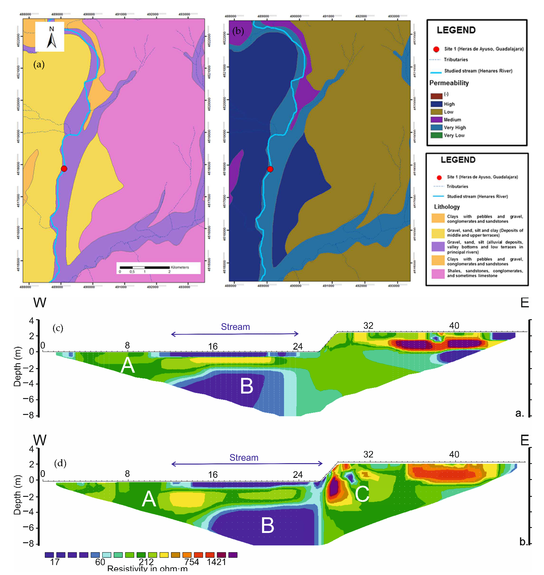
The copepod assemblages of the HEN and TAJ were significantly correlated (ρ = 0.694; p-value: 0.049) to a combination of five chemico-physical variables, namely TSS, NPOC, K, V coarse%, and V fine %; accordingly, the marginal tests of DISTLM highlighted that the granulometry played a role in shaping the copepod assemblages (V.fine %: p = 0.035; Fine%: p = 0.002; Medium %: p = 0.431; V. coarse%: p = 0.007) together with K (p = 0.024), and TSS (p = 0.012).
The SIMPER analysis output indicated 77% (Heras de Ayuso, Henares River) (Romanones, Tajuna River) of the sub-basin. Contrib%: percentage of dissimilarity provided by each species; Cum%: cumulative percentage of dissimilarity.

3.4. ERT Profiles

The RMS absolute error of the ERT images obtained at the HEN Site during mild and cold seasons were 3.9% and 5.2%, respectively. The inversion procedure reached convergence after the five (June 2013) and seven (April 2014) iterations. The river deposits at this site, characterized by gravel, sand, and silt alluvial sediments (Figure 6a,b), showed a modest resistivity variability due to the season, since the values ranged from 15–5000 Ohm.m in the June 2013 period (Figure 6c) and from 14–3100 Ohm.m during the April 2014 (Figure 6d). ERT also indicated the presence of a permeable zone up to 0.5 m thick (A), thus including the hyporheic zone as a whole. The permeable zone proved to extend laterally for ca. 5 m from the channel. A low-resistivity (<70 Ohm.m) permeable zone (B) below the streambed and unconnected with the river channel was detected during both surveys, but at different depths (2.3 m and 3 m, respectively); however, the channel appears to be slightly connected with the aquifer in the April 2014 (after intense floods), via lateral terrace located to the east (Figure 6d).
The ERT profiles carried out at the TAJ site display RMS absolute errors of 2.0% and 1.4% for June 2013 and April 2014, respectively (Figure 7). In both cases, a convergence during the inversion procedure was achieved after seven iterations. Gravel, sand, and silt mixed with marl sediments with gypsum crusts characterize the geological materials present at the site (Figure 7a,b).
The overall resistivity variability due to the season ranges from 10–600 Ohm.m during the June 2013 (Figure 7c) to 3–1400 Ohm.m during the April 2014 (Figure 7d). Looking at the mean resistivity values obtained around the stream location, the resistivity is lower in April 2014 indicating a high content in water of the sediments at that time. Both profiles showed a low-permeability zone (D) from the benthic up to 0.5 m of the profile (thus including the hyporheic zone), with resistivity values ranging from 45 to 80 Ohm.m (Figure 7c,d).
Similar to the HEN site, a low-resistivity (<50 Ohm.m) permeable zone (E) appears below the streambed, disconnected with the river channel and at a different depth depending on the time of the experiment (2.3 m and 3 m, respectively). Furthermore, a low-resistivity (<30 Ohm.m) high-permeability zone (F) was detected 2 m laterally from the riverbed, at a depth of ca. 3 m. This zone would be associated either to a suspended aquifer supplied with water from the terraces (located to the west-northeast west of the profile), or to water accumulation within tree roots, that might be temporarily connected with the stream’s hyporheic system.

4. Discussion

Quantifying the extent of the sediment structure and the water flow in the hyporheic zone of temporary rivers, in combination with the biotic communities, is a particularly challenging issue with significant implications for a stream’s ecosystem management [4,12,63,64]. For temporary streams located in the Mediterranean region, this is a particular concern, given that they are exceedingly prone to the alteration of environmental conditions due to climatic shifts and the intensification of drought periods. These events are predicted to change the hyporheic zone’s sediment configuration and subsequently the organizational pattern of the hyporheic communities [65,66,67].
Our experimental investigations performed in two gaining rivers from the upper Tagus River Watershed (Guadalajara Province) demonstrate the effectiveness of the ERT application technique to depict the physical characteristics of the HZ at the local scale and to delineate its vertical and lateral extent in conjunction with the analyses of structural pattern of the hyporheos. We also found that the permeability of the riverbed sediments detected at the local scale in both rivers is in contrast with the overall permeability previously detected at the catchment scale in the Jarama basin [25,26]. These results confirm previous studies on the hyporheic system, indicating that the local-scale permeability is higher than that of the surrounding catchment [68] and vary spatially.
The hyporheic zone material in the HEN site in the Henares River is dominated by gravels and coarse sands, showing a low-resistivity ranging from 20–80 Ohm.m and indicating a relatively high-permeability. Consequently, there is a high-surface input, and a low-residence time of the water into a hyporheic zone, indicating a more active interstitial water renewal, shown by the similar values of 18O for both surface and HZ waters. Below the stream bed, at 2.3 m, there was a low-permeability area detected with a resistivity of <70 Ohm.m associated with the shallow floodplain aquifer of Guadalajara. In June 2013, this area was not connected to the river. This fact is likely due to a general lowering of the piezometric level in the Guadalajara aquifer in the summer that may be leading to a reduction in the base flow of the Henares watercourse [38,69].
At this site, the relationships between the hyporheic biota and the water’s physico-chemistry are correlated just for copepod assemblages, indicating that other factors might be responsible for controlling the structural patterns of the whole hyporheic community.
We assume that the differences in sediment porosity and permeability due to grain size are prone to seasonal alterations of the particularities of the fluvial sediment’s deposits and to changes in the surface channel flow (vertical connection), significantly altering the configuration of the hyporheos. At this site the hyporheic biota is dominated by non-stygobite species, mostly benthic, indicating more significant surface water input into the hyporheic zone. The low abundance of the stygobites species Eucyclops hadjebensis and Acanthocyclops n. sp. (the later found also in the associated alluvial aquifer) indicate that the connection to the river with the alluvial aquifer may occur only sporadically throughout the year [26,69].
The hyporheic zone material at the TAJ site in the Tajuña River is dominated by coarse to very fine sands in a silty–argillaceous matrix variably cemented by gypsum. Similarly, as in the previous case, the water chemistry influences have low significance on the structural pattern of hyporheic communities. The ERT results shows a low-permeability zone in the upper 0.5 m of the profile, with resistivity values ranging from 45–80 Ohm.m. The obtained ERT profile indicates a reduced hyporheic zone extension in both vertical and lateral dimensions. Here, both water retention into the hyporheic sediments and the interaction between water and sediments are higher than at the HEN site and consequently, the hyporheic water is slightly more mineralized (Table S1, Supplementary Materials) [26,36,69]. During both experimental periods, below the streambed of the Tajuña, there was a high-permeability zone detected with low resistivity (<30 Ohm.m) located at 3 m depth and 2 m laterally from the channel in the riparian zone. This area might be associated with either a suspended aquifer supplied with water from the terraces of the Tajuña River, or with the water accumulation within tree roots. This area was slightly connected with the stream-hyporheic system of the river in June 2013.
Although the alluvial aquifer of La Alcarria is assumed to be hydraulically connected with Tajuña River, the connection was not detected during our experiments. This might be the results of the high accumulation of total suspended solids in the HZ (more evident in June 2013) that could significantly contribute to clogging the hyporheic interstices and would further impede the hydraulic connection with the alluvial aquifer, blocking the pathways to reach the hyporheic zone by obligate-groundwater species. The presence of a mixture of coarse, medium and fine sand is also an indication of the low-discharge capacity of the aquifer to reach the hyporheic zone during the experimental period [36]; however, when compared to the site of the Henares River, the hyporheic site of Tajuña River appears to exchange the water with the associated alluvial aquifer more frequently. This might be predicted by the incidence of an abundant stygobite population of Parastenocaris sp. 2 during the two ERT experimental periods and the presence of a second stygobite dweller during the 2-year monitoring period, i.e., Acanthocyclops sp. [26,36,69]. We assume that the configuration of hyporheic sediments at this site allows for the presence of a ‘subsurface highway’, enabling stygobites species to reach the streambed in certain periods of the year.
The hyporheic residents respond to the perceived fine-scales dynamics of water exchanges by the establishment of large stygobite populations during the year which are resilient to changes of hyporheic environmental conditions when the contact with the alluvial aquifer is lost. Fine sediments are usually one of the major sources of physical-habitat deterioration with negative consequences on many ecological processes of the river [70]; however, the presence of fine sediments and a high-residence time of the water generates a range of environmental conditions suitable for the persistence of stygobite species.

Implication of Hyporheic Zone Biota as Indicators for Surface–Groundwater Exchanges: From Theory to Practice

The potential use of hyporheic biota as biological tracers for water movement and surface—groundwater exchanges has long been recognized [4,26,34]. The earliest published studies attempting to delineate the hyporheic zone are actually based on biota [71]. In these studies, it was first assumed that the hyporheic sediments do not function only as a refugee space for surface dwellers against disturbances caused by extreme droughts or floods events [72], but rather, that the hyporheic zone is a stable environment for specific fauna. The hyporheic zone was later documented to be populated by a complex and dynamic meiofauna [73,74,75] which are moving deeper beneath the streambed and up to a few hundreds of meters from the channel into the alluvial plain [71], which discounts the theory that they are occasional refugees from the surface channel.
It is highly relevant to define the average depth of the hyporheic biota distribution into the HZ, which sometimes proved to extend up to 3 km from the river [76]. It was also shown that the distribution and structure of hyporheic communities are more subjective to the direction and magnitude of water flow [77], groundwater flow and/or exchange with the stream [78], the sedimentary structure of alluvial sediments [36,79,80], and geological terrains [81] rather than to environmental conditions of water [26,82,83,84]. Clogging also markedly influenced the hyporheic biota. Density and taxonomic richness are reduced in logged catchments; whereas in unlogged basins, the hyporheos were denser and extended at greater depths. The HZ structure is shaped by water flow, but a significant contribution can result from the combined interaction among water, sediments and biota, which enhance the ecological integrity of fluvial ecosystems.

5. Conclusions

This paper sought to demonstrate the congruence of the ERT and ecological techniques in describing the hydrological characteristics of the hyporheic zone at the local scale. In particular, we examined the properties of the hyporheic zone of two groundwater-fed streams from the upper part of Tagus River watershed. We found that a non-invasive ERT image coupled with biological and hydrological assessments of the hyporheic zone provide enough important information related to the structure and configurations of the sediments and their properties to characterize the habitat provided by this zone and its connection with the associated alluvial aquifer. We identify that the hyporheic biota has a similar taxonomic richness at both sites; however, there are significant differences among the structural pattern configuration independent of the physico-chemical parameters of the water. Hence, the site dominated by coarse and very coarse sand with a high permeability allows for a more active surface–hyporheic water exchange and low-water retention into the sediments. This is characterized by a combination of cosmopolitan surface species, mostly benthic, and few stygobites in low abundance. In contrast, the hyporheic site characterized by less permeable sediments and a more interaction among sediments and waters, has a distinct configuration of the hyporheos being best represented by stygobyte taxa. Our overall results provide initial templates for high-resolution in situ studies with broad and integrated methods to identify the boundaries between hyporheic and parafluvial zones and the time-scale fluctuations in response to water exchanges with the surface stream.

Supplementary Materials

The following material are available online at: https://www.mdpi.com/article/10.3390/w14213396/s1, Table S1: Environmental variables measurements in the study sites (Site 1, HEN—Heras de Ayuso, Henares River; Site 2, TAJ—Romanones, Tajuna River (Guadalajara, central Spain); Table S2: Mean total and taxon-specific invertebrates’ abundances and higher-level taxon richness in Site 1, HEN (Heras de Ayuso, Henares River) and Sites 2, TAJ (Romanones, Tajuna River); Table S3: List of copepods and ostracods from the hyporheic zone of the two investigated sites, Sites 1, HEN—Henares River and Site 2, TAJ—Tajuna River (central Spain) between 2012–2014; Figure S1: Non metric multidimensional scaling (nMDS) plot of samples from the two investigated sub-basins (HEN—Heras de Ayuso, Henares River; and TAJ—Romanones, Tajuna River) based on copepod abundances.

Author Contributions

Conceptualization, S.I.; methodology, S.I., D.G.-O., J.L.-R, R.R.-L., and T.D.L.; software, D.G.-O.; validation, S.I., D.G.-O., J.L, and R.R.-L.; formal analysis, S.I., D.G.-O., J.L, and T.D.L.; investigation, S.I., D.G.-O., J.L, R.R.-L., and T.D.L.; resources, S.I., D.G.-O., J.L., and R.R.-L.; data curation, S.I.; writing—original draft preparation, S.I.; writing—review and editing, S.I., D.G.-O., J.L., R.R.-L., and T.D.L.; visualization, S.I. and D.G.-O.; supervision, S.I. All authors have read and agreed to the published version of the manuscript.

Institutional Review Board Statement

Not applicable.

Informed Consent Statement

Not applicable.

Data Availability Statement

The data presented in this study are available in Supplementary Materials.

Conflicts of Interest

The authors declare no conflict of interest.

References

  1. Orghidan, T. Un nou domeniu de viata acvatica subterana: ‘biotopul hiporeic’. Bul. Stiintific Sect. Biol. Stiinte Agric. 1955, 7, 657–676. [Google Scholar]
  2. Bencala, K.E. Hyporheic zone hydrological processes. Hydrol. Process. 2000, 14, 2797–2798. [Google Scholar] [CrossRef]
  3. Braun, A.; Auerswald, K.; Geist, J. Drivers and Spatio-Temporal Extent of Hyporheic Patch Variation: Implications for Sampling. PLoS ONE 2012, 7, e42046. [Google Scholar] [CrossRef] [PubMed] [Green Version]
  4. Leigh, C.; Stubbington, R.; Sheldon, F.; Boulton, A.J. Hyporheic invertebrates as bioindicators of ecological health in temporary rivers: A meta-analysis. Ecol. Indic. 2013, 32, 62–73. [Google Scholar] [CrossRef] [Green Version]
  5. Gibert, J.; Dole-Olivier, M.-J.; Marmonier, P.; Vervier, P. Surface water-groundwater ecotones. In he Ecology and Management of Aquatic-Terrestrial Ecotones; Naiman, R.J., Decamps, H., Eds.; UNESCO Parthenon Publishing: London, UK, 1990. [Google Scholar]
  6. Boulton, A.J.; Datry, T.; Kasahara, T.; Mutz, M.; Stanford, J.A. Ecology and management of the hyporheic zone: Stream-groundwater interactions. J. N. Am. Benthol. Soc. 2010, 29, 26–40. [Google Scholar] [CrossRef] [Green Version]
  7. Triska, F.J.; Kennedy, V.C.; Avanzino, R.J.; Zellweger, G.W.; Bencala, K.E. Retention and transport of nutrients in a third-order stream in northwestern California: Hyporheic processes. Ecology 1989, 70, 1893–1905. [Google Scholar] [CrossRef]
  8. Kautz, R.; Kawula, R.; Hoctor, T.; Comiskey, J.; Jansen, D.; Jennings, D.; Kasbohm, J.; Mazzotti, F.; McBride, R.; Richardson, L.; et al. How much is enough? Landscape-scale conservation for the Florida panther. Biol. Conserv. 2006, 130, 118–133. [Google Scholar] [CrossRef]
  9. Krause, S.; Hannah, D.M.; Fleckenstein, J.H.; Heppell, C.M.; Pickup, R.; Pinay, G.; Robertson, A.; Wood, P.J.; Kaeser, D. Inter-disciplinary perspectives on processes in the hyporheic zone. Ecohydrology 2011, 4, 481–499. [Google Scholar] [CrossRef] [Green Version]
  10. McGarr, J.T.; Wallace, C.D.; Ntarlagiannis, D.; Sturmer, D.M.; Soltanian, M.R. Geophysical mapping of hyporheic processes controlled by sedimentary architecture within compound bar deposits. Hydrol. Process. 2021, 35, e14358. [Google Scholar] [CrossRef]
  11. Palmer, M.A.; Ambrose, R.F.; Poff, N.L. Ecological Theory and Community Restoration Ecology. Restor. Ecol. 1997, 5, 291–300. [Google Scholar] [CrossRef] [Green Version]
  12. Boulton, A.J.; Findlay, S.; Marmonier, P.; Stanley, E.H.; Valett, H.M. The functional significance of the hyporheic zone in streams and rivers. Annu. Rev. Ecol.Syst. 1998, 29, 59–81. [Google Scholar] [CrossRef]
  13. Malcolm, I.A.; Soulsby, C.; Youngson, A.F.; Petry, J. Heterogeneity in ground water–surface water interactions in the hyporheic zone of a salmonid spawning ground. Hydrol. Process. 2004, 17, 601–617. [Google Scholar] [CrossRef]
  14. Stonedahl, S.H.; Harvey, J.W.; Harvey, J.W.; Salehin, M.; Packman, A.I. A multiscale model for integrat-ing hyporheic exchange from ripples to meanders. Water Resour. Res. 2010, 46. [Google Scholar] [CrossRef] [Green Version]
  15. Stubbington, R. The Hyporheic Zone as A Refugium for Benthic Invertebrates in 589 Groundwater-Dominated Streams. Ph.D. Thesis, Loughborough University, Loughborough, UK, 2011. [Google Scholar]
  16. Boulton, A.J.; Fenwick, G.D.; Hancock, P.J.; Harvey, M.S. Biodiversity, functional roles and ecosystem services of groundwater invertebrates. Invert. Syst. 2008, 22, 103–116. [Google Scholar] [CrossRef]
  17. Iepure, S.; Kalache, M.; Rasines-Ladero, R. Land-use influence on hyporheic biota from Mediterranean streams in central Spain. Studia UBB Ambientum 2020, 16, 13–42. [Google Scholar] [CrossRef]
  18. Zarnetske, J.P.; Haggerty, R.; Wondzell, S.M.; Baker, M.A. Labile dissolved organic carbon supply limits hyporheic denitrification. J. Geophys. Res. 2011, 116, G04036. [Google Scholar] [CrossRef] [Green Version]
  19. Brosten, T.R.; Bradford, J.H.; McNamara, J.P.; Gooseff, M.N.; Zarnetske, J.P.; Bowden, W.B.; Johnston, M.E. Multi-offset GPR methods for hyporheic zone investigations. Near Surf. Geophys. 2009, 7, 247–257. [Google Scholar] [CrossRef] [Green Version]
  20. Ward, A.S.; Schmadel, N.M.; and Wondzell, S.M. Time-Variable Transit Time Distributions in the Hyporheic Zone of a Headwater Mountain Stream. Water Resour. Res. 2018, 54, 2017–2036. [Google Scholar] [CrossRef]
  21. Busato, L.; Boaga, J.; Perri, M.T.; Majone, B.; Bellin, A.; Cassiani, G. Hydrogeophysical characterization and monitoring of the hyporheic and riparian zones: The Vermigliana Creek case study. Sci. Total Environ. 2019, 648, 1105–1120. [Google Scholar] [CrossRef]
  22. Dole-Olivier, M.J.; Marmonier, P.; Beffy, J.L. Response of invertebrates to lotic disturbance: Is the hyporheic zone a patchy refugium? Freshw. Biol. 1997, 37, 257–276. [Google Scholar] [CrossRef]
  23. Hancock, P.J. Human impacts on the stream–groundwater exchange zone. Environ. Manag. 2002, 29, 763–781. [Google Scholar] [CrossRef] [PubMed]
  24. Dole-Olivier, M.J.; Castellarini, F.; Coineau, N.; Galassi, D.M.P.; Martin, P.; Mori, N.; Valdecasas, A.; Gibert, J. Towards an optimal sampling strategy to assess groundwater biodiversity: Comparison across six European regions. Freshw. Biol. 2009, 54, 777–796. [Google Scholar] [CrossRef]
  25. Iepure, S.; Martinez-Hernandez, V.; Herrera, S.; Rasines-Ladero, R.; de Bustamante, I. Response of microcrustacean communities from the surface-groundwater interface to water contamination in urban river system of the Jarama basin (central Spain). Environ. Sci. Pollut. Res. 2013, 20, 5813–5826. [Google Scholar] [CrossRef] [PubMed]
  26. Iepure, S.; Meffe, R.; Carreño, F.; Rasines-Ladero, R.; de Bustamante, I. Geochemical, geological and hydrological influence on ostracod assemblages distribution in the hyporheic zone of two Mediterranean rivers in central Spain. Int. Rev. Hydrobiol. 2014, 99, 435–449. [Google Scholar] [CrossRef]
  27. Bork, J.; Berkhoff, S.E.; Bork, S.; Hahn, H.J. Using subsurface metazoan fauna to indicate groundwater–surface water interactions in the Nakdong River floodplain, South Korea. Hydrol. J. 2009, 17, 61–75. [Google Scholar] [CrossRef]
  28. Stoch, F.; Artheau, M.; Brancelj, A.; Galassi, D.M.P.; Malard, F. Biodiversity indicators in European ground waters: Towards a predictive model of stygobiotic species richness. Freshwat. Biol. 2009, 54, 745–755. [Google Scholar] [CrossRef]
  29. Stein, H.; Kellermann, C.; Schmidt, S.I.; Brielmann, H.; Steube, C.; Berkhoff, S.E.; Fuchs, A.; Hahn, H.J.; Thulin, B.; Griebler, C. The potential use of fauna and bacteria as ecological indicators for the assessment of groundwater quality. J. Environ. Monit. 2010, 12, 242–254. [Google Scholar] [CrossRef]
  30. Galassi, D.M.P.; Lombardo, P.; Fiasca, B.; Di Cioccio, A.; Di Lorenzo, T.; Petitta, M.; Di Carlo, P. Earthquakes trigger the loss of groundwater biodiversity. Sci. Rep. 2014, 4, 6273. [Google Scholar] [CrossRef] [Green Version]
  31. Petitta, M.; Caschetto, M.; Galassi, D.M.P.; Aravena, R. Dualflow in karst aquifers toward a steady discharge spring (Presciano, central Italy): Influences on a subsurface groundwater dependent ecosystem and on changes related to post-earthquake hydrodynamics. Environ. Earth Sci. 2015, 73, 2609–2625. [Google Scholar] [CrossRef]
  32. Mori, N.; Kanduč, T.; Opalički Slabe, M.; Brancelj, A. Groundwater drift as a tracer for identifying sources of spring discharge. Groundwater 2015, 53, 123–132. [Google Scholar] [CrossRef]
  33. Stoch, F.; Fiasca, B.; Di Lorenzo, T.; Porfirio, S.; Petitta, M.; Galassi, D.M.P. Exploring copepod distribution patterns at three nested spatial scales in a spring system: Habitat partitioning and potential for hydrological bioindication. J. Limnol. 2016, 75, 1–13. [Google Scholar] [CrossRef]
  34. Boulton, A.J.; Humphreys, W.F.; Eberhard, S.M. Imperiled subsurface waters in Australia: Biodiversity, threatening processes and conservation. Aquat. Ecosys. Health 2003, 6, 41–54. [Google Scholar] [CrossRef]
  35. Moldovan, O.T.; Levei, E.; Banciu, M.; Banciu, H.L.; Marin, C.; Pavelescu, C.; Brad, T.; Cimpean, M.; Meleg, I.; Iepure, S.; et al. Spatial distribution patterns of the hyporheic invertebrate communities in a polluted river in Romania. Hydrobiologia 2011, 669, 63–82. [Google Scholar] [CrossRef]
  36. Rasines-Ladero, R.; Iepure, S. Parent lithology and organic matter influence hyporheic biota from two mediterranean rivers in central Spain. Limnetica 2016, 35, 19–36. [Google Scholar]
  37. AEMET. Available online: https://www.aemet.es/ (accessed on 1 June 2013).
  38. IGME. Available online: https://www.ign.es/web/resources/sismologia/tproximos/sismotectonica/pag_sismotectonicas/bet_centro.html (accessed on 1 February 2015).
  39. Arribasa, J.; Critelli, S.; Le Pera, E.C.; Tortosaa, A. Composition of modem stream sand derived from a mixture of sedimentary and metamorphic source rocks (Henares River, Central Spain). Sediment. Geol. 2000, 133, 27–48. [Google Scholar] [CrossRef] [Green Version]
  40. Benitez-Mora, A.; Camargo, J.A. Ecological Responses of Aquatic Macrophytes and Benthic Macroinvertebrates to Dams in the Henares River Basin (Central Spain). Hydrobiologia 2014, 728, 167–178. [Google Scholar] [CrossRef]
  41. Telford, W.M.; Geldart, L.P.; Sheriff, R.E.; Keys, D.A. Applied Geophysics, 2nd ed.; Cambridge University Press: Cambridge, UK, 1990; p. 770. [Google Scholar]
  42. Reynolds, J.M. An Introduction to Applied Environmental Geophysics; Wiley: New York, NY, USA, 1997; p. 780. [Google Scholar]
  43. Sasaki, Y. Resolution of resistivity tomography inferred from numerical simulation. Geophys. Prospect. 1992, 40, 453–464. [Google Scholar] [CrossRef]
  44. Loke, M.H. Electrical Imaging Surveys for Environmental and Engineering Studies. A Pract. Guide 2-D 3-D Surv. 2000, 61. [Google Scholar]
  45. Loke, M.H.; Wilkinson, P.B.; Chambers, P.B.; Strutt, M. Optimized arrays for 2-D cross-borehole electrical tomography surveys: Geophys. Prospect. 2014, 62, 172–189. [Google Scholar]
  46. Loke, M.H.; Acworth, I.; Dahlin, T. A comparison of smooth and blocky inversion methods in 2D electrical imaging surveys. Explor. Geophys. 2003, 34, 182–187. [Google Scholar] [CrossRef] [Green Version]
  47. Bernard, J. The Depth of Investigation of Electrical Methods; IRIS-instruments: Orléans, France, 2003. [Google Scholar]
  48. Malard, F.; Dole-Olivier, M.J.; Mathieu, J.; Stoch, F. Sampling manual for the assessment of regional groundwater biodiversity. In Sampling Manual Published within the Framework of the EU Project PASCALIS (Protocols for the ASsessment and Conservation of Aquatic Life In the Subsurface); EU: Maastricht, The Netherlands, 2002. [Google Scholar]
  49. Meisch, C. Freshwater Ostracoda from Western and Central Europe Süβwasserfauna von Mitteleuropa; Spektrum Akademischer Verlag: Heidelberg, Germany, 2000. [Google Scholar]
  50. Dussart, B.; Defaye, D. World Directory of Crustacea Copepoda of Inland Waters II—Cyclopiformes; Backhuys Publishers: Leiden, The Netherlands, 2006. [Google Scholar]
  51. Gibert, J.; Danielopol, D.L.; Stanford, J.A. Groundwater Ecology; Academic Press Inc.: San Diego, CA, USA, 1994. [Google Scholar]
  52. Anderson, M.J. A new method for non-parametric multivariate analysis of variance. Austral Ecol. 2008, 26, 32–46. [Google Scholar] [CrossRef]
  53. McArdle, B.H.; Anderson, M.J. Fitting Multivariate Models to Community Data: A Comment on Distance-Based Redundancy Analysis. Ecology 2001, 82, 290–297. [Google Scholar] [CrossRef]
  54. Gower, J.C. Some Distance Properties of Latent Root and Vector Methods Used in Multivariate Analysis. Biometrika 1966, 53, 325–338. [Google Scholar] [CrossRef]
  55. Kennedy, P. A Guide to Econometrics, 4th ed.; MIT Press: Cambridge, MA, USA, 1998. [Google Scholar]
  56. Chao, A. Non-parametric estimation of the number of classes in a population. Scand. J. Stat. 1984, 11, 265–270. [Google Scholar]
  57. Ugland, K.I.; Gray, J.S.; Ellingsen, K.E. The Species-Accumulation Curve and Estimation of Richness. J. Anim. Ecol. 2003, 72, 888–897. [Google Scholar] [CrossRef]
  58. Colwell, R.K.; Rahbek, C.; Gotelli, N. The mid-domain effect and species richness patterns: What have we learned so far? Am. Nat. 2004, 163, E1–E23. [Google Scholar] [CrossRef] [Green Version]
  59. Chao, A.; Lee, S.M. Estimating the number of classes via sample coverage. J. Am. Stat. Assoc. 1992, 87, 210–217. [Google Scholar] [CrossRef]
  60. Yek, S.H.; Williams, S.E.; Burwell, C.J.; Robson, S.K.A.; Crozier, R.H. Ground dwelling ants and surrogates for establishing conservation priorities in the australian wet tropics. J. Insects Sci. 2009, 9, 12. [Google Scholar] [CrossRef] [Green Version]
  61. Clarke, K.R. Non-parametric multivariate analysis of changes in community structure. Austral. J. Ecol. 1993, 18, 117–143. [Google Scholar] [CrossRef]
  62. Clarke, K.R.; Somerfield, P.J.; Gorley, R.N. Exploratory null hypothesis testing for community data: Similarity profiles and biota-environment linkage. J. Exp. Mar. Biol. Ecol. 2008, 366, 56–69. [Google Scholar] [CrossRef]
  63. McDonough, T.O.; Hosen, J.; Plamer, M. Temporary streams: The hydrology, geopgraphy and ecology of non-perennially flowing waters. In River Ecosystems: Dynamics, Management and Conservation, Hannah, S., Elliot, Lucas, E., Martin, Eds.; Nova Science Publishers, Inc.: Hauppauge, NY, USA, 2011; ISBN 978-1-61209-145-7. [Google Scholar]
  64. Sanchez-Hernandes, J.; Nunn, A.D. Environmental changes in a Mediterranean river: Implications for the fish assemblage. Ecohydrology 2016, 9, 1439–1451. [Google Scholar] [CrossRef]
  65. Bonada, N.; Rieradevall, M.; Dallas, H.; Davis, J.; Day, J.; Figueroa, R.; Resh, V.H.; Prat, N. Multi-scale assessment of macroinvertebrate richness and composition in Mediterranean-climate rivers. Freshw. Biol. 2008, 53, 772–788. [Google Scholar] [CrossRef]
  66. Dole-Olivier, M.-J.; Maazouzi, C.; Cellot, B.; Fiers, F.; Galassi, D.M.P.; Claret, C.; Marmonier, P. Assessing invertebrate assemblages in the subsurface zone of stream sediments (0–15 cm deep) using a hyporheic sampler. Water Resour. Res. 2014, 50, 453–465. [Google Scholar] [CrossRef]
  67. Nikolaidis, N.P.; Demetropoulou, L.; Froebrich, J.; Jacobs, C.; Gallart, F.; Prat, N.; Lo Porto, A.; Campana, C.; Papadoulakis, V.; Skoulikidis, N.; et al. Towards sustainable management of Mediterranean river basins: Policy recommendations on management aspects of temporary streams. Water Policy 2013, 15, 830–849. [Google Scholar] [CrossRef] [Green Version]
  68. Storey, R.; Howard, K.; Williams, D. Factors controlling rifflescale hyporheic exchange flows and their seasonal changes in a gaining stream: A three-dimensional groundwater flow model, Water Resour. Res. 2003, 39, 1034. [Google Scholar] [CrossRef]
  69. Rasines-Ladero, R. The Ecology of the Hyporheic Zone Associated with the Rivers Henares and Tajuña (Jarama River Basin, Spain). Ph.D. Thesis, University Rey Juan Carlos, Madrid, Spain, 2017. [Google Scholar]
  70. Iepure, S.; Rasines, R.; Meffe, R.; Carreño, F.; Mostaza, D.; Sundberg, A.; di Lorenzo, T.; Barroso, J. Exploring the distribution of groundwater Crustacea (Copepoda and Ostracoda) to disentangle aquifer type features—A case study in the upper Tajo basin (Central Spain). Ecohydrology 2017, 10, e1876. [Google Scholar] [CrossRef]
  71. Buendia, C.; Gibbins, C.N.; Vericat, D.; Batalla, R.J. Reach and catchment-scale influences on invertebrate assemblages in a river with naturally high fine sediment loads. Limnologica 2013, 43, 362–370. [Google Scholar] [CrossRef]
  72. Danielopol, D.L. Groundwater fauna associated with riverine aquifers. J. N. Am. Benthol. Soc. 1989, 8, 18–35. [Google Scholar] [CrossRef]
  73. Schwoerbel, J. Die Bedeutung des Hyporheals fur “gerollfu” hrender Hochgebirgsba¨che mit bewegter gewa¨ssers. Verh. Der Int. Ver. FuR Theor. Und Angew. Limnol. 1964, 15, 215–226. [Google Scholar]
  74. Ward, J.V.; Bretschko, G.; Brunke, M.; Danielopol, D.L.; Gibert, J.; Gonser, T.; Hildrew, A.G. The boundaries of river systems: The metazoan perspective. Freshw. Biol. 1998, 40, 531–569. [Google Scholar] [CrossRef]
  75. Robertson, A.; Rundle, S.D.; Schmid-Araya, J.M. An introduction to a special issue on lotic meiofauna. Freshw. Biol. 2000, 44, 1–3. [Google Scholar] [CrossRef]
  76. Marmonier, P.; Archambaud, G.; Belaidi, N.; Bougon, N.; Breil, P.; Chauvet, E.; Claret, C.; Cornut, J.; Datry, T.; Dole-Olivier, M.J.; et al. The role of organisms in hyporheic processes: Gaps in current knowledge, needs for future research and applications. Ann. Limnol.-Int. J. Lim. 2012, 48, 253–266. [Google Scholar] [CrossRef]
  77. Stanford, J.A.; Ward, J.V. The Hyporheic Habitat of River Ecosystems. Nature 1988, 335, 64–66. [Google Scholar] [CrossRef]
  78. Hakenkamp, C.C.; Palmer, M.A. The ecology of hyporheic meiofauna. In Streams and Ground Waters; Jones, J.B., Mulholland, P.J., Eds.; Academic Press: London, UK, 2000. [Google Scholar]
  79. Stanley, E.H.; Boulton, A.J. Hydrology and the distribution of hyporheos: Perspectives from a mesic river and a desert stream. J. N. Am. Benthol. Soc. 1993, 12, 79–83. [Google Scholar] [CrossRef]
  80. Trayler, K.M.; Davis, J.A. Forestry impacts and the vertical distribution of stream invertebrates in southwestern Australia. Freshw. Biol. 1998, 40, 331–342. [Google Scholar] [CrossRef]
  81. Dumas, P.; Bou, C.; Gibert, J. Groundwater macrocrustaceans as natural indicators of the Ariége alluvial aquifer. Int. Rev. Hydrobiol. 2001, 86, 619–633. [Google Scholar] [CrossRef]
  82. Cannan, C.E.; Armitage, P.D. The influence of catchment geology on the longitudinal distribution of macroinvertebrate assemblages in a groundwater dominated river. Hydrol. Process. 1999, 13, 355–369. [Google Scholar] [CrossRef]
  83. Malard, F.; Tockner, K.; Dole-Olivier, M.-J.; Ward, J.V. A landscape perspective of surface–subsurface hydrological exchanges in river 30 corridors. Freshw. Biol. 2002, 47, 621–640. [Google Scholar] [CrossRef]
  84. Malard, J.; Adamowski, J.; Días, M.R.; Yax, H.T.; Arévalo-Rodríguez, L.A.; Melgar-Quiñonez, H. Agroecological food webs: Modelling a missing piece to climate change adaptation. Geophys. Res. Abstr. 2019, 21, EGU2019-11656. [Google Scholar] [CrossRef]
Figure 1. Hyporheic reach—scale exchange pattern associated with ripples, bars, and meanders, adapted from [14].
Water 14 03396 g001
Figure 2. Location of the study sites in Madrid region (central Spain), HEN—Herras de Ayuso (Henares River) and TAJ—Romanones (Tajuna River).
Water 14 03396 g002
Figure 3. Pictures showing the main features of the investigated sites; (ac) Heras de Ayuso (Site 1, HEN, Henares River), (d) Romanones (Site 2, TAJ, Tajuna River).
Water 14 03396 g003
Figure 4. Principal coordinate analysis (PCO) plot of samples from the investigated sub-basin: Site 1 (a) (HEN—Heras de Ayuso, Henares River) and Site 2 (b) (TAJ—Romanones, Tajuna River) based on environmental parameters (abbreviations as in Table 1).
Water 14 03396 g004
Figure 5. Species rarefaction curves and estimators’ curves for copepods and ostracods in the groundwater of Upper Tagus River Watershed at increasing sample size. (Sobs): species rarefaction curve of observed species richness (mean values estimated by mean of 999 randomizations without replacement). Non-parametric estimators: Chao1, Chao2, Jacknife1, Jacknife2, Bootstrap and UGE; parametric estimator: MM (Michaelis–Menten), based on the number of collected samples.
Water 14 03396 g005
Figure 6. Characteristics of the hyporheic zone at Heras de Ayuso (Site 1) Henares River. (a) lithology; (b) permeability; (c) ERT applied in June 2013; (d) ERT applied in April 2014.
Water 14 03396 g006
Figure 7. Characteristics of the of the hyporheic zone at Romanones, Tajuna River. (a) lithology; (b) permeability; (c) ERT applied in June 2013; (d) ERT applied in April 2014.
Water 14 03396 g007
Table 1. Variables used for the analysis in the test area.
Variables Units/Indices
GeographicalAltitude (m a.s.l.)
Lithology
HydrologyWater depth (m)
Channel width (m)
Surface water discharge (m/s)
Surface water discharge (m/s monthly average)
Chemico-physicalConductivity (μS/cm, EC)
Non-purgeable organic carbon (in mg/L−1, NPOC)
Total carbon (TC)
Inorganic carbon (IC)
Total organic carbon (mg/L−1, TOC)
Dissolved organic carbon (mg/L−1, DOC)
Total suspended solids (mg/L−1, TSS)
Total alkalinity (mg/L−1, as HCO3)
Cations Mg2+, K+, Ca2+
Major anions Cl, SO42−, NO3
Biological Total abundance of species
Species richness (SR)
Stygobites number (SB)
Non-stygobites number (nSB)
Statistical levels Sub-basins (SUB): Henares (HEN), Tajuna (TAJ)
Habitats (HAB): surface (SW), hyporheic zone (HYPORHEIC ZONE) Season (SEA): cold (C), mild (M)
Table 2. Environmental variables and biotic parameters in the investigated sites.
Sites/
Environmental Variables
Site 1
Hera de Ayuso (HEN)
Site 2
Romanones (TAJ)
SW/HWJune 2013April 2014June 2013April 2014
Depth (cm)SW
HW
Water discharge * (m/s)SW2.642.50.460.48
Water discharge (m/s monthly average)SW2.833.60.520.49
Temperature (°C)SW15.6±13.23±11.86±6.43±
HW16.75±13.75±12.45±7.1±
Dissolved O2 (mg/L)SW 10.6±12.46±
HW8.91± 8.45±10.14±
pHSW8.04±8.4±8.36±8.1±
HW8.17±8.24±8.15±7.7±
Conductivity (μS/cm)SW1107±1024±549.3±736.6±
HW1102.5±1017±555±779.5±
ER (Ohm)HW19.1–73.7 47.9–77.5
Biotic parameters
Total abundance *HZ 5954041951226
Species richness ** HZ 9638
Stygobites ** HZ 3201
Non-stygobitesHZ 6437
Note(s): * without Ostracoda caparaces; ** Copepoda, Ostracoda), SW—surface water; HW—hyporheic water; HZ—hyporheic zone.
Table 3. SIMPER dissimilarity between the two investigated sites, Heras de Ayuso (Site 1, HEN) (Henares River) and Romanones (Site 2, TAJ) (Tajuna River).
SpeciesContrib%Cum.%
Paracyclops imminutus16.3516.35
Bryocampthus sp. 212.4728.81
Microcyclops rubellus11.6240.43
Macrocyclops albidus11.5051.94
Diacyclops languidoides lang. ssp11.2263.16
Microcyclops sp.7.4170.57
Parastenocaris sp.16.6377.20
Publisher’s Note: MDPI stays neutral with regard to jurisdictional claims in published maps and institutional affiliations.

