An Artificial Neural Network Model for Water Quality and Water Consumption Prediction

Abstract

With rapid urbanization, high rates of industrialization, and inappropriate waste disposal, water quality has been substantially degraded during the past decade. So, water quality prediction, an essential element for a healthy society, has become a task of great significance to protecting the water environment. Existing approaches focus predominantly on either water quality or water consumption prediction, utilizing complex algorithms that reduce the accuracy of imbalanced datasets and increase computational complexity. This study proposes a simple architecture of neural networks which is more efficient and accurate and can work for predicting both water quality and water consumption. An artificial neural network (ANN) consisting of one hidden layer and a couple of dropout and activation layers is utilized in this regard. The approach is tested using two datasets for predicting water quality and water consumption. Results show a 0.96 accuracy for water quality prediction which is better than existing studies. A 0.99 $R^2$ score is obtained for water consumption prediction which is superior to existing state-of-the-art approaches.

1. Introduction

Water quality directly impacts the health of human beings as it can be used for cooking, drinking, agriculture, etc. [1]. Similarly, it has a strong impact on other types of life and a potential impact on the ecosystem. Apart from drinking, water is used for power generation, navigation, recreation, etc. [2]. Water is the most essential resource for life on Earth, and the survival of existing organisms and human life is tied to it. Water of appropriate quality and its ready availability are primary requirements for living creatures. Species living in the water can tolerate a certain amount of pollution, but highly polluted or dirty water has a potential impact on their existence, putting their lives at high risk. The quality of most ambient water bodies, such as rivers, lakes, and streams, is determined by precise quality standards [3]. Water specifications for various applications/use also have their own sets of standards. For example, irrigation water must not be overly saline, nor should it contain poisonous elements; passing such water to plants and crops can destroy ecosystems. Based on the industrial processes, water quality for industrial uses also requires different properties. Natural water resources, such as ground and surface water, are some of the cheapest sources of fresh water [4]. Human/industrial activity, as well as other natural processes, can pollute such resources.

Water scarcity is a burning issue for many countries [5]. By the end of this decade, half of the world population is predicted to be living in water-stressed areas [6]. Water consumption prediction and water quality classification hold great significance in managing the sustainability of water distribution systems [6]. Water consumption prediction is a very important factor for infrastructure decision makers. Such predictions are very helpful in devising plans to meet the future needs for efficient water use in urban areas where large expansions are underway. Furthermore, water consumption prediction is necessary to foresee the needs for future smart cities, where smart and efficient water consumption is expected to reduce energy use and resources [7].

Rapid and large industrial development during the past decade led to increased water consumption. In addition, water quality has deteriorated at an alarming rate. Furthermore, infrastructures have a considerable impact on the use and quality of water due to a lack of public knowledge and fewer hygienic attributes. Indeed, the effects of excessive use of water and its contamination are quite harmful, threatening the very existence of human life, the environment, and infrastructure. According to a United Nations (UN) report, about 1.5 million people die each year from diseases caused by contaminated/dirty water [8]. Reports indicate that 80% of health problems in developing countries are caused by contaminated water. Five million deaths and 2.5 billion illnesses are reported yearly [9], which is much higher than all the deaths caused by accidents, terrorist attacks, crimes, etc.

Therefore, water quality and water consumption monitoring are necessary to alleviate the impact of polluted and dirty water. Water quality and its demand can be checked using traditional methods such as manually collecting water samples and then analyzing them using different techniques. However, these techniques are time-consuming and costly. Sensors might also be considered a traditional technique. However, using sensors to assess all of the water quality and its consumption prediction is deemed expensive and typically results in low precision. Predictive modeling using machine learning and deep learning algorithms is another option for monitoring water consumption and its quality. It has several advantages over other traditional methods, including cheaper costs, efficiency in terms of travel and collection time, the ability to predict under various phases of a system, and the capability to predict ideal values when accessing a site is difficult.

Many researchers have used neural networks and other machine learning methods in the field of water quality classification and its consumption prediction in recent years and have obtained good results. With this motivation, this work uses the water quality index (WQI), a collection of diverse water quality metrics that depicts water quality. Different parameters are used for forecasting water consumption, and both prediction and classification models are applied to predict the water quality and its consumption. In addition, the following are the paper’s main contributions:

• An approach is proposed which can work for both water quality prediction and water consumption forecasting. For this purpose, the architecture of an artificial neural network is deployed to obtain high performance with less complexity.
• For performance analysis of the proposed approach, several machine learning models are employed, including random forest (RF), decision tree (DT), extra tree (ET) classifier, logistic regression (LR), support vector machine (SVM), and AdaBoost (ADA) classifier. Moreover, a convolutional neural network (CNN), long short-term memory (LSTM), gated recurrent unit (GRU), and artificial neural network (ANN) are also used for performance appraisal.
• Performance is measured using accuracy, precision, recall, and F1 score. Moreover, root means squared error (RMSE), mean absolute error (MAE), mean square error (MSE), and $R^2$ are also used. A single model with high accuracy for both water quality prediction and water consumption forecasting is developed. Several existing state-of-the-art approaches are also used for performance validation.

The following is the structure of this paper. The literature review is presented in Section 2. The architecture of the proposed models is introduced in Section 3, along with a brief overview of the machine and deep learning models used. Section 4 presents the experimental setup and the analysis of the results. Finally, the paper is concluded in Section 5, and limitations and future scope are given.

2. Literature Review

This research explores the existing literature that has employed different approaches to solve the problems related to water quality. Typically, statistical and lab analyses are used to determine water quality, while developments in artificial intelligence (AI) help in finding the optimized solution for the water quality problem.

Theyazn et al. [10] used deep learning models, non-linear auto regression neural networks (NARNET), LSTM, machine learning models, support vector machine (SVM), k-nearest neighbors (KNN), and naïve Bayes (NB) for water quality classification. They achieved an accuracy value of 97.01% using the machine learning algorithm SVM. Hasan and Alhammadi [11] used standard water physical and chemical data from the Abu Dhabi water department for monitoring drinking water quality. The authors used five machine learning algorithms, such as LR, naive Bayes (NB), DT, SVM, and k-nearest neighbor (KNN). Results show that the DT was more efficient than other classifiers for the water quality level prediction and achieved an accuracy of 97.70%.

The study [12] adopted dimension reduction techniques to extract the most dominant parameters from the data. The authors used principal component regression (PCR) methods and machine learning algorithms in the proposed approach for water quality prediction. For the PCR method, accuracy of 95% was obtained, while a 100% accuracy was achieved by using the machine learning algorithm gradient boosting classifier. Dilimi and Ladjal [13] proposed a system for water quality classification. The proposed system integrates deep learning models with feature extraction to obtain better results. To estimate the performance of the LSTM and recurrent neural networks (RNNs) the authors used two methods of out-of-sample test and three methods of cross-validation. They demonstrated an accuracy value of 99.72% by using LSTM-RNN with latent Dirichlet allocation (LDA) and LSTM-RNNs with independent component analysis (ICA) using the random holdout technique.

The water quality classification system in [14] employed machine learning algorithms SVM, DT, and NB. The weighted arithmetic water quality index (WAWQI) was used to train the machine learning algorithms. The achieved accuracy was 98.50% using the DT classifier. Hassan et al. [15] worked on the prediction of water quality using BTM, SVM, MN, RF, and multiple linear regression (MLR). The proposed approach follows a five-step process, including preprocessing of data, handling missing values, feature correlation, machine learning algorithms, and models feature importance. A maximum accuracy of 99.83% was obtained using the MLR classifier. Haq et al. [16] followed a machine-learning-based approach for predicting water quality. Two types of performance were compared in this work. For the evaluation of the machine learning model, the study used K-fold cross-validation. The highest accuracy of 97.23% was achieved with the DT classifier.

Kouadri et al. [17] proposed a machine-learning-based system for predicting the water quality index of the Illizi region (Algerian southeast). The study performed two types of experiments following all features and reduced features based on sensitivity analysis. In the first scenario, MLR achieved 1, 1.4572 × 10–08, 3.1708 × 10–08%, 1.2573 × 10-10%, and 2.1418 × 10–08% for R, MAE, root relative squared error (RRSE), relative absolute error (RAE), and RMSE, respectively. For the second scenario, RF achieved 0.9984, 5.9642, 1.9942, 4.693, and 3.2488 for R, RRSE, MAE, RAE, and RMSE, respectively. Adhaileh and Alsaade [18] worked on the water quality index (WQI) and water quality prediction using the adaptive neuro-fuzzy interface (ANFIS) and KNN, and feed-forward neural network (FFNN), respectively. The study achieved a 100% accuracy for water quality classification using FFNN and 96.17% for the WQI using ANFIS with a regression coefficient. Umair et al. [19] used machine learning algorithms for the WQI and water quality classification using 15 machine learning algorithms and achieved good results. Gradient boosting and polynomial regression predicted the WQI with an MAE of 1.9642 and 2.7273, respectively. For water quality classification, MLP achieved an 85.07% accuracy score.

Baudhaouia and Wira’s work [20] presented data analysis for water consumption in real time using deep learning techniques. For the prediction of water consumption, they used LSTM and a backpropagation neural network (BPNN). LSTM achieved an RMSE value of 0.13, and BPNN achieved an RMSE value of 0.48. Shuang and Zhao [21] used the Beijing–Tianjin–Hebei region annual water report data to predict water demand for a particular region. They used eleven statistical-based and machine-learning-based models to conduct the study. To find the most suitable predictive models, they used two predictive scenarios: interpolation prediction scenario (IPS) and extrapolation prediction scenario (EPS). Results demonstrate that the GBDT achieved good performance in both scenarios. In addition to water quality prediction, several studies investigated water evolution in different regions. For example, ref. [22] utilized the isotopic and hydrogeochemical data of the karstic region to study water evolution. Different clustering methods were employed in this regard. The models were used to find the categorization of geological, hydrogeochemical, and isotopic characteristics. Similarly, ref. [23] studies the ground level of water using simulations by employing soft computing models. The objective was to consider meteorological components, such as precipitation, temperature, and evapotranspiration, and analyze their impact on the water level. Results demonstrated that ANN, fuzzy logic, adaptive neuro-fuzzy inference system, and least-square support vector machine models can be used to simulate the ground level of water.

Aggarwal and Sehgal [24] conducted a comparative study using machine learning algorithms with attribute selection techniques, fold cross-validation, and preprocessing techniques. The authors used lasso regression, ridge regression, XGBoost, least-square SVM, and the hybrid model (Lasso regression+XGBoost). Results proved that the proposed hybrid model achieved good results. Smolak et al. [25] used classical and adaptive algorithms for short-term water consumption prediction. The authors used ET, RF, support vector regression, autoregressive integrated moving averages (ARIMA), and blind techniques. Results showed that RF achieved an accuracy of 90.4% (measured by the mean absolute percentage error). Guo and Liu [26] only used two deep learning models GRU and conventional artificial neural network (ANN) for short-term water demand prediction. To simulate a real-life situation, they used two predictive approaches: a 15 min prediction and 24 h prediction with a 15 min time step. The result showed that the GRU outperformed the ANN model for both simulation scenarios.

Predominantly, the above-discussed research does not estimate the water quality classification based on accuracy, F1 score, etc.. Nor does it use too many parameters to obtain better results. Similarly, several approaches work either on WQI or water quality classification which necessitates a system that can work well with water quality classification and water demand prediction. The proposed methodology improved these notations by using a lightweight model. Table 1 shows a comparative summary of the discussed research works.

Table 1. Comparative summary of the discussed research works.

Ref.	Year	Classifiers	Achieved Accuracy	Dataset
[10]	2020	NARNET, LSTM, SVM, KNN, NB	SVM 97.01%	https://www.kaggle.com/anbarivan/indian-water-quality-data (Access on 20 July 2022).
[11]	2021	LR, NB, DT, SVM, KNN	DT 97.70%	Abu Dhabi Department of Energy dataset
[12]	2021	RF, SVC, GBC, ADA	GBC 100%	Gulshan Lake dataset
[13]	2021	Dimension reduction PCA, LDA, ICA RNN, LSTM, SVM (variants)	99.72% LSTM RNN with LDA LSTM RNN with ICA	Tilesdit Dam dataset
[27]	2020	SVM, DT, NB	DT 98.50%	(I) Narmada River, state of Madhya Pradesh, India (II) Combined data for the historical water quality of certain locations in India.
[15]	2021	NN, RF, MLR, SVM, BT	99.83% MLR	Indian water quality data on Kaggle
[16]	2021	DT, NB (variants), K-fold cross-validation	97.22% DT	https://www.kaggle.com/adityakadiwal/water-potability (Access on 20 July 2022).
[17]	2021	MLR, RF, M5PTree, RSS, AR, ANN, SVR, LWLR	With all parameters: MLR R = 1, MAE = 1.4572 × 10–08, RMSE = 2.1418 × 10–08, RAE = 1.2573 × 10–08%, RRSE = 3.1708 × 10–08% With reduced parameters based on the sensitivity analysis: RF R = 0.9984 MAE = 1.9942 RMSE = 3.2488 RAE = 4.693 RRSE = 5.9642	Illizi region of Algeria, state of Illizi directorate of water resource dataset.
[18]	2021	KNN, FFNN, ANIFS	WQI ANFIS 96.17% WQC FFNN 100%	https://www.kaggle.com/anbarivan/indian-waterquality-data (Access on 23 July 2022)
[19]	2019	Multiple linear regression, polynomial regression, RF, GBC, SVM, ridge regression, lasso regression, elastic net regression, MLP, GNB, LR, SGD, KNN, DT, bagging classifier	Classification: MLP accuracy = precision = recall = F1-score = regression: With 4 parameters GBC MAE = 1.9642 MSE = 7.2011 RMSE = 2.6835 R-squared = 0.7485 With 3 parameters: polynomial regression MAE = 2.7273 MSE = 12.7307 RMSE = 3.5680 R-squared = 0.4851	Rawal water lake dataset, Pakistan Council of Research in Water Resources (PCRWR) (available online at URL http://www.pcrwr.gov.pk/ (Access on 23 July 2022))
[20]	2021	LSTM,BPNN	LSTM RMSE = 0.13 BPNN RMSE = 0.48	Domestic house water consumption in France
[21]	2021	Linear regression, ridge regression, lasso regression,kernel ridge regression,baysian ridge regression, BPNN,DT, SVM, RF, Ada Boost, GBDT	GBDT (IPS) MSE = 0.00000016 MAE = 0.00032787 $R^2$ = 99.999% (EPS) MSE = 0.00006178 MAE = 0.00584230 $R^2$ = 99.9578%	BEIJING–Tianjin–Hebei region annual water report
[24]	2021	XGBoost, LSSVR, lasso regression, ridge regression, Proposed (Lasso regression + XGBoost)	proposed (lasso regression+XGBoost) MAE = 1.75 ADERV = 0.0591	Water consumption in the New York City, @city-of-ny, on data.world
[25]	2020	ET, RF,SVR, ARIMA/ARIMAX, Blind	RF Accuracy = 90.4%	Wroclaw water consumption report, Poland
[26]	2018	GRU, ANN	GRU 15 min MAE = 1.44 RMSE = 1.97 Nash–Sutcliffemodel efficiency = 0.991 mean absolute percentage error = 2.02 24 h MAE = 3.67 RMSE = 5.16 Nash–Sutcliffemodel efficiency = 0.941 mean absolute percentage error = 4.79	Changzhou city China

3. Methodology

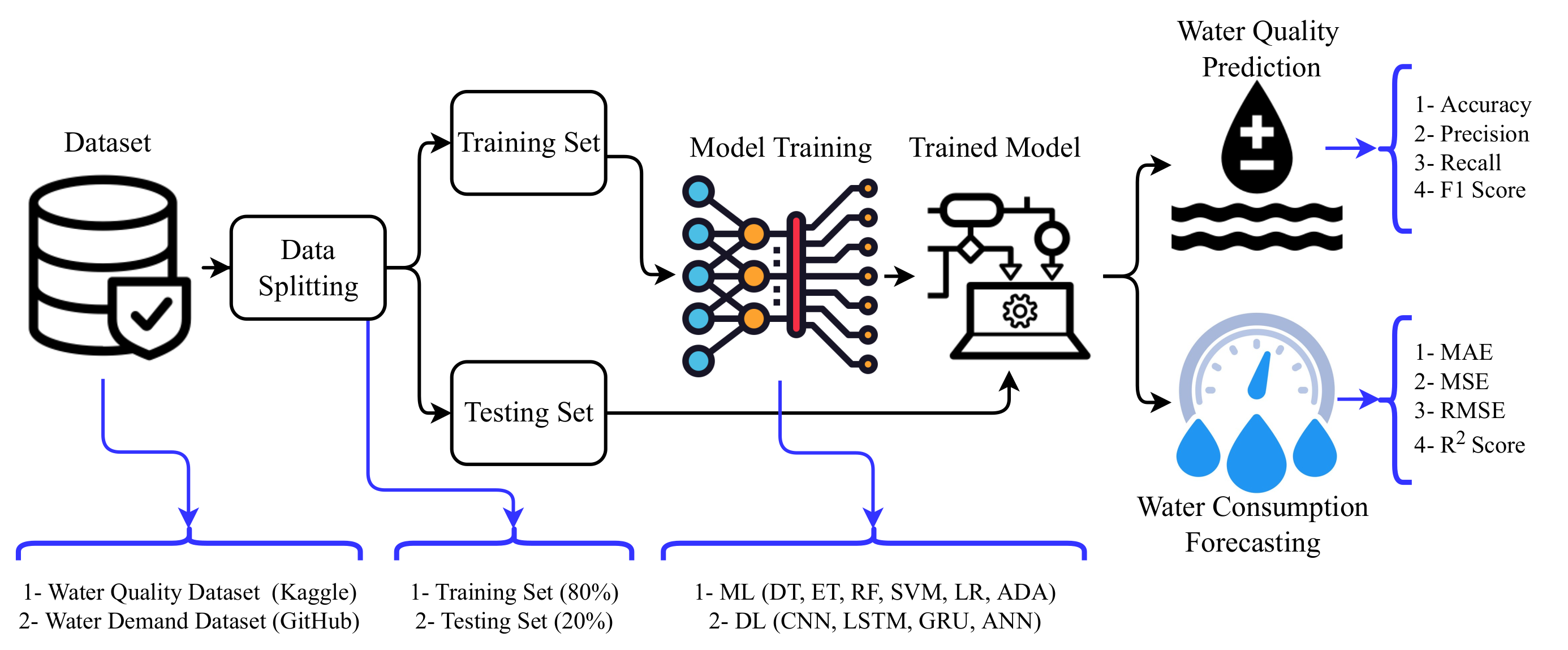
This study works on the prediction of water quality and forecasting of water consumption using a machine learning approach. From that perspective, it leverages state-of-the-art techniques for the chosen problem. To train machine learning models for both water consumption and water quality prediction, two datasets were acquired: the water quality prediction dataset from Kaggle [28] and the water consumption dataset from GitHub [29]. Experiments were performed using machine learning models RF, DT, ET, LR, SVM, and ADA and deep learning models CNN, LSTM, and GRU to compare their performance with the proposed approach. This study proposes a simple, yet efficient model for water quality and water consumption prediction. Figure 1 shows the flow of the methodology used in this study. Models are evaluated in terms of accuracy, precision, recall, F1 score, and confusion matrix for water quality prediction, while water consumption prediction is evaluated regarding RMS, MAE, and $R^2$. The study follows the steps of dataset acquiring, training machine learning models, and performance evaluation. A brief discussion of each is provided in the following sections.

Figure 1. Architecture of the adopted methodology in this study.

3.1. Datasets

This study used two datasets; one for water quality prediction and the other for water consumption forecasting. The datasets employed to conduct this research were acquired from renowned sources such as Kaggle and GitHub.

3.1.1. Water Quality

For water quality classification, the dataset was acquired from Kaggle [28]. This dataset consists of 8000 samples and 21 attributes. All the attributes of the water quality dataset are variables. A detailed description of the dataset variables is provided in Table 2.

Table 2. Description of attributes of water quality dataset.

No.	Attribute	Description	Range per Liter
1	aluminum	Water is unsafe if the level of aluminum is greater than 2.8 per liter	[0–5.05]
2	ammonia	Water is unsafe if the level of ammonia is greater than 32.5 per liter	[−0.08–29.8]
3	arsenic	Water is unsafe if the level of arsenic is greater than 0.01 per liter	0–1.05
4	barium	Water is unsafe if the level of barium is greater than 2 per liter	0–4.94
5	cadmium	Water is unsafe if the level of cadmium is greater than 0.005 per liter	0–0.13
6	chloramine	Water is unsafe if the level of chloramine is greater than 4 per liter	0–8.68
7	chromium	Water is unsafe if the level of chromium is greater than 0.1 per liter	0–0.9
8	copper	Water is unsafe if the level of copper is greater than 1.3 per liter	0–2
9	fluoride	Water is unsafe if the level of fluoride is greater than 1.5 per liter	0–1.5
10	bacteria	Water is unsafe if the level of bacteria is greater than 0 per liter	0–1
11	viruses	Water is unsafe if the level of viruses is greater than 0 per liter	0–1
12	lead	Water is unsafe if the level of lead is greater than 0.015 per liter	0–0.2
13	nitrates	Water is unsafe if the level of nitrates is greater than 10 per liter	0–19.8
14	nitrites	Water is unsafe if the level of nitrites is greater than 1 per liter	0–2.93
15	mercury	Water is unsafe if the level of mercury is greater than 0.002 per liter	0- 0.1
16	perchlorate	Water is unsafe if the level of perchlorate is greater than 56 per liter	0 - 60
17	radium	Water is unsafe if the level of radium is greater than 5 per liter	0–7.99
18	selenium	Water is unsafe if the level of selenium is greater than 0.5 per liter	0 – 0.1
19	silver	Water is unsafe if the level of silver is greater than 0.1 per liter	0–0.5
20	uranium	Water is unsafe if level of uranium is greater than 0.3 per litre	0–0.9
21	is_safe	class attribute (target class)	0 = not safe 1 = safe

Table 3 shows a few sample records from the dataset where `is_safe’ is the target class and has two values 0 and 1 for `not safe’ and `safe’ water, respectively.

Table 3. Sample records from water quality dataset.

No.	Selenium	Silver	Uranium	…	Is_Safe
1	0.08	0.34	0.02		1
2	0.08	0.27	0.05		1
3	0.07	0.44	0.01		0

Figure 2 shows the distribution of 20 attributes of the dataset which includes the amount of aluminum, ammonia, arsenic, etc. for safe and not-safe classes. The ratio between safe and not-safe classes is different and these features can be used to predict the water quality.

Figure 2. Distribution of water-containing compounds from the dataset.

3.1.2. Water Consumption Forecast

The dataset used for the water consumption forecast consists of two variables which are `Date’ and `Consumption’. The ’Date’ variable contains the timestamp, while the `Consumption’ variable contains the water consumption corresponding to that date. Table 4 shows the samples from the water-forecasting dataset.

Table 4. Sample records from water consumption dataset.

No.	Date	Consumption
1	7 January 2009	108,637.2762
2	7 February 2009	108,638.8474
3	7 March 2009	108,633.8275

Figure 3 shows the water consumption records for the last 10 years indicating that the demand varies between 80,000 to 130,000 in the city of London, Canada. In addition to the ups and downs over the years, the water demand has increased as well.

Figure 3. Trends of water consumption for city of London, Canada, from 2010 to 2020 [29].

3.2. Machine Learning Algorithms

For the classification of water quality, this study used several machine learning algorithms, a brief description of which is provided here for completeness. Machine learning models for water quality prediction and water consumption prediction are also discussed in terms of the parameter setting in Table 5 and Table 6, respectively. These hyperparameter settings were obtained using the grid search method which means that we tuned machine learning models between a specific range.

Table 5. Classifier hyperparameters setting for water quality prediction.

Model	Hyperparameters	Hyperparameters Tuning
DT	max_depth = 50	max_depth = {5 to 200}
RF	max_depth = 50, n_estimators = 300	max_depth = {5 to 200}, n_estimators = {50 to 500}
ETC	max_depth = 50, n_estimators = 300	max_depth = {5 to 200}, n_estimators = {50 to 500}
ADA	learning_rate = 0.8, n_estimators = 300	learning_rate = {0.1 to 1.0}, n_estimators = {50 to 500}
SVC	Kernel = linear, C = 1.0	Kernel = {poly, linear, sigmoid} C = {1.0 to 5.0}
LR	solver = liblinear, C = 1.0	Kernel = {liblinear, saga, sag} C = {1.0 to 5.0}

Table 6. Regression models hyperparameters setting for water consumption prediction.

Model	Hyperparameters	Hyperparameters Tuning
DT	max_depth = 10	max_depth = {2 to 50}
RF	max_depth = 10, n_estimators = 300	max_depth = {2 to 50}, n_estimators = {50 to 500}
ETC	max_depth = 10, n_estimators = 300	max_depth = {2 to 50}, n_estimators = {50 to 500}
ADA	learning_rate = 0.8, n_estimators = 300	learning_rate = {0.1 to 1.0}, n_estimators = {50 to 500}
SVR	kernel=’poly’	Kernel = {poly, linear, sigmoid}
LR	Default	Default

3.2.1. Decision Tree

A DT processes information in the form of trees which can also be represented as a set of discrete rules [30]. DT’s main advantage is its use of decision rules and features subsets that arise at various classification stages. A DT is made up of various nodes, including a leaf node and a number of internal nodes with branches. Every leaf node indicates a class that corresponds to an example, whereas internal nodes represent features, and branches represent a combination of features that leads to classification. The performance of the DT is determined by how well it is built on the training set. For the current study, the max_depth parameter was used with a value of 50 indicating that each tree can grow to a maximum of 50-level depth. It is used to help reduce the complexity of tree construction.

3.2.2. Random Forest

RF is a tree-based machine learning model that combines the results obtained by fitting several DTs on randomly selected training samples [31]. To select a root node, each DT in RF is built using an indicator such as information gain, or gini-index. RF is a meta-estimator that can be used for regression as well as classification tasks. RF’s prediction accuracy can be improved with the number of trees. By using the bootstrap sampling techniques, RF overcomes the overfitting problem [32]. RF was deployed with two hyperparameters as shown in Table 5. The n_estimators variable was used with a value of 300 which include 300 DTs in the prediction procedure. The max_depth parameter was used as a 50 indicating the maximum level to which each tree can grow.

3.2.3. Logistic Regression

LR is a statistical-based classification algorithm that is based on the sigmoid function or logistic function. LR maps between the given set of input features by sigmoid function with a discrete set of target variables by probability approximation. The sigmoid function is an S-shaped curve that restricts the probability value between the target variables [33]. Table 5 shows the hyperparameters used for LR including the ’liblinear’ solver which is a more suitable optimization algorithm for small datasets.

3.2.4. Support Vector Classifier

SVC is a linear model and is widely used for classification tasks [34]. SVC uses the data points to map them in a space of n dimensions, where n represents the number of features. It finds the ’best fit’ hyperplane that can differentiate between classes and performs classification. This study uses the SVC with a linear kernel as well as another parameter C = 3.0 as the regularization value.

3.2.5. Extra Tree Classifier

ETC is an ensemble machine learning approach that is based on DTs and is practically identical to an RF classifier. In ETC, however, randomization is generated through random divisions of data instead of bootstrapping input. It may enhance variance since bootstrapping diversifies it [11].

3.2.6. AdaBoost

ADA is an ensemble machine learning method that uses the boosting technique. Using this method, the weights are re-allocated for every instance; high weights are associated with improperly categorized instances. Boosting is applied to minimize the biases and variations in values. Basically, it is based on the concept of sequentially growing learning. In other words, the poor learner is transformed into a strong learner. During the process of training, it constructs various DTs. When the first DT is constructed, the wrongly classified record is prioritized and forwarded to the next DT. The procedure is repeated up to the number of provided basic learners [10].

3.3. Deep Learning Models

Recently, the use of deep learning models has gained wide attention. This study also deploys several deep learning models for performance comparison and analysis of results. A comprehensive description of these algorithms is provided in this part.

3.3.1. Convolutional Neural Network

CNN is a renowned deep learning model that handles data complexity during computation very well. Convolutional layers, dropout layer, activation layers, a flatten layer, and a pooling layer make up the CNN model. In CNN, the main layer is the convolutional layer, which extracts features, while the pooling layer reduces the size of these extracted features, the dropout layer reduces the overfitting, and the flatten layer transforms the data into an array.

3.3.2. Long Short-Term Memory Network

LSTM is a deep learning model specifically designed to handle classification problems. LSTM is an extended version of a recurrent neural network (RNN). With the help of memory cells and three gates, LSTM effectively saves information and handles long sequences. To control memory cells, it employs structured gates to add and forget data. To decide which information to delete, a forget gate is used [35]. The purpose of the sigmoid function is to remember the information if the output is 1 and forgot it if the output is 0. It is performed in light of current and previous states.

3.3.3. Gated Recurrent Unit

There are two versions of RNN; one is LSTM, and another variant of RNN is GRU, which is basically similar to LSTM. However, unlike LSTM, which has three layers, there are two layers in a GRU [12]. The first gate, called the reset gate, mainly manages the combination of previous computations and new input. The second gate, known as dubbed update gate, regulates what kind of information or data should be kept from the previous computations. GRU is mainly known as the conventionalized LSTM model and is more effective in terms of computational power compared to vanilla RNN and LSTM.

3.4. Proposed Artificial Neural Network Architecture

ANN is a non-linear computational model that has played a vital role in the field of machine learning. It is based on the working mechanism of a biological neural network. Similar to the linked neurons of the human brain, an ANN is made up of a large number of linked neurons. These neurons are capable of learning, generalizing training data, and deriving conclusions from complex data [36]. Usually, ANN consists of three interconnected layers: an input layer, a hidden layer(s), and an output layer. The input layer receives the input patterns/information for learning and then passes it to the hidden layer. The hidden layer contains the set of neurons that perform calculations on the input data. It learns the hidden patterns using ’weights’ which consist of the ’sum of weighted synapse connections’. Let, $h_1$ and $h_2$ be the input containing $w_1$ and $w_2$ weights, then the dot product of inputs and weight values will be calculated as $h_1·w_1+h_2·w_2$. In brief, the weighted sum is computed by the ANN, which also incorporates a bias b. It will become $h_1·w_1+h_2·w_2+b$. Bias is added to the model to avoid overfitting. There can be several hidden layers in an ANN. It removes the redundancy from input data and then forwards it to the next hidden layer for more computations. In this activation function, $A_f$ is used to convert the input signal into the output signal. The activation function is applied because the nature of solvable problems includes numerous influential aspects. It uses sigmoid and softmax transfer functions in the hidden and output layers, respectively. The third layer is the output layer which contains the model’s output/conclusions produced from all calculations. This layer can have a single or several nodes. The binary classification problem contains only one node and produced output [0 or 1]. The multi-class classification problem contains more than one node and produces output for more than one classification problem [37].

There are two types of ANN: one is an FFNN while the other is an RNN. The FFNN is a simple and most basic kind of ANN where the flow of the data is unidirectional, the input layer forwards data to the hidden layer, and the hidden layer forwards it to the output layer. FFNN is further divided into two types: single-layer perceptron (no hidden layer) and multi-layer perceptron (one or more than one hidden layer) [38]. The multi-layer perceptron can learn both linear and non-linear functions. Let h be the number of inputs with m units, then

$$h=h_1,h_2,\dots ,h_m\parallel hϵR^m$$

(1)

Then, randomly initialized weights are:

$$w=w_1,w_2,\dots ,w_m$$

(2)

As mentioned earlier, the hidden layer receives input and calculates the dot-product of h and w, called pre-state $S_p$, which can be calculated as

$$S_p=h_1.w_1+h_2.w_2+,\dots ,+b=\sum _{n=1}^m{W}_n*X_n+b$$

(3)

where m shows the total number of nodes, and b is the bias.

Equation (3) shows that the weighted sum of input is passed to an activation function. The activation function is used for the calculation of the non-linearity of the model. The whole process is represented in a matrix form. The calculations of the hidden layer are computed using different m numbers of pre-state $S_p^m$. In the end, the output is produced after applying the activation function. The activation function is applied on these pre-state $S_p^m$, which is called a state P of a neuron It is represented as

$$P=\alpha (W_m·S_p^m+b_m)$$

(4)

Let $(h^1,y^1),(h^2,y^2),\dots ,(h^m,y^m)$ be the input pairs, where $h^m$ indicates the input data point, and $y^m$ is a target point. The building of $NN$ will be

$$N\left(h^m\right)=y^m$$

(5)

Then, the error ${ϵ}_m$ will be calculated as

$$O^m=N\left(h^m\right),m$$

(6)

$$y^m=O^m+{ϵ}_m$$

(7)

where $O^m$ denotes the output that depends on various parameters. After that, the operations are performed to minimize the error rate as follows

$$E=\frac{1}{T}\sum _{m=1}^p\left|\right|y^m-O^m{\left|\right|}^2$$

(8)

where T is the various training parameters, E denotes the functions, and p denotes the data pairs

$$\left|\right|y^m-O^m{\left|\right|}^2={(y_1-O_1)}^2+{(y_1-O_1)}^2+,\dots ,+{(y_p-O_p)}^2$$

(9)

As we know, we cannot change the input and output values because these are assigned values. Now, by performing differentiation of both sides,

$$\frac{\delta }{\delta W}\left|\right|y-{O\left|\right|}^2=-2(Y-O)·\frac{\delta 0}{\delta W}$$

(10)

By using the chain rule, it becomes

$$\frac{\delta }{\delta W_{mj}}\left(\right||y-{O\left|\right|}^2)=-2(Y_m-O_m)·h_j$$

(11)

where $h_j$ shows that it is inside the mth coordinate location.

This returns as the output of $NN$ with different values of error rates. To make good estimations, we need a large amount of data. The crucial point is that once we obtain the derivative of the sum of squares error, we can use the training practice to alter these weights accordingly.

Figure 4 shows the architecture of the proposed ANN model. For classification and future forecasting, ANN consists of seven layers. The first layer is a dense layer containing 256 neurons that takes input data to perform calculations and then passes it to the rectified linear unit (ReLU) activation layer which creates linearity in the feature set. We used ReLU because it is simple, fast, and performs well for non-linear data. After the activation layer, we used a dropout layer with a 0.5 dropout rate which randomly deletes 50% of the neurons from the network to reduce complexity in the model. The second dense layer, after the dropout layer, contains 256 neurons followed by the ReLU activation layer and dropout layer with a 0.5 dropout rate. In the end, for the water quality layer, we used a dense layer with two neurons, and for water consumption prediction we used a dense layer with a single neuron. For water consumption prediction, we compiled the model with the `Adam’ optimizer and `mean_squared_error’ loss function, while for water quality prediction we compiled the model with the `Adam’ optimizer and binary_crossentropy loss function.

Figure 4. Architecture of proposed ANN model.

3.5. Performance Evaluation Metrics

Performance evaluation of the trained machine learning and deep learning models was carried out to understand how good the developed model was. To evaluate the performance of the aforementioned models, confusion matrix-based evaluation parameters were considered. For the water quality classification, we used accuracy, precision, recall, and F1 Score. The values of these parameters range between [0, 1], and they are calculated as follows

$$Accuracy=\frac{TP+TN}{TP+TN+FP+FN}$$

(12)

where TP, TN, FP, and FN represent the true positive, true negative, false positive, and false negative, respectively.

$$Precision=\frac{TP}{TP+FP}$$

(13)

$$Recall=\frac{TP}{TP+FN}$$

(14)

$$Precision=2*\frac{Precision*Recall}{Precision+Recall}$$

(15)

For water consumption prediction, we used MAE, MSE, RMSE, and RSE with the following equations

$$MAE=\frac{\sum (\parallel \parallel x_{obs}-x_{pred}\parallel \parallel )}{n}$$

(16)

$$MSE=\frac{\sum {(x_{obs}-x_{pred})}^2}{n}$$

(17)

$$RMSE=\sqrt{\frac{\sum {(x_{obs}-x_{pred})}^2}{n}}$$

(18)

$$R^2=1-\frac{\left(ExplainedVariation\right)}{\left(TotalVariation\right)}$$

(19)

4. Results and Discussions

The results for water quality prediction and water quality consumption are described in this section. These results were obtained by deploying machine learning and deep learning models. Experiments were performed using an Intel Core i7, a 7th generation machine with a Windows operating system. We used Python version 3+ and Jupyter notebook. The dataset was split into 0.8 to 0.2 ratios for training and testing, respectively.

4.1. Results for Water Quality Prediction

Models were used to predict the water quality as `safe’ or `not safe’ using machine learning, deep learning, and the proposed model. Table 7 shows experimental results for water quality prediction for machine learning models. Results suggest that most of the machine learning models perform better.

Table 7. Experimental results for the machine learning models.

Model	Accuracy	Class	Precision	Recall	F1 Score
LR	0.90	0	0.91	0.98	0.95
		1	0.68	0.28	0.39
		Avg.	0.80	0.63	0.67
DT	0.95	0	0.97	0.97	0.97
		1	0.77	0.78	0.78
		Avg.	0.87	0.88	0.87
RF	0.95	0	0.96	0.99	0.97
		1	0.91	0.65	0.76
		Avg.	0.93	0.82	0.87
SVM	0.91	0	0.91	0.99	0.95
		1	0.72	0.28	0.40
		Avg.	0.82	0.63	0.67
ADA	0.93	0	0.94	0.99	0.96
		1	0.82	0.50	0.62
		Avg.	0.88	0.74	0.79
ETC	0.92	0	0.92	1.00	0.96
		1	0.96	0.29	0.45
		Avg.	0.94	0.65	0.70

Tree-based models perform significantly better in terms of accuracy and F1 scores compared to linear models, such as DT which achieved a 0.95 accuracy and 0.87 F1 scores. Similarly, RF also achieved a 0.95 accuracy with a 0.87 F1 score. These models do not show higher overfitting on imbalanced data compared to linear models because tree-based models do not need a large dataset for training, so a few samples from the minority class are enough for the tree-based models. Linear models, such as LR and SVM, also perform well in terms of accuracy scores and achieved 0.90 and 0.91 accuracy scores, respectively. However, regarding the F1 score, both had poor performance, each with a 0.67 score. Linear models need a large dataset for training so they obtain a good fit for majority class data but are underfit for minority class data.

For the most part, the models experienced overfitting on the majority class data and showed poor performance for minority class samples. Because of the models’ overfitting, the accuracy score of models was much higher compared to the F1 score. Models showed substantially better results for the `not safe’ (0) class prediction as each model achieved almost similar results for precision, recall, and F1 score. However, for the `safe’ class (1), models showed poor performance in terms of each evaluation parameter because of underfit. Models did not receive enough training samples for the `safe’ class during training and showed poor performance for the minority class.

Figure 5 shows the confusion matrix for the machine learning models. In the confusion matrix, axis values 0 and 1 represent the `not safe’ and `safe’ targets, respectively. RF showed the best performance regarding the number of correct predictions with 1525 correct predictions out of 1600 predictions and gave only 75 wrong predictions. It is followed by the DT with 1419 correct predictions and 81 wrong predictions, while LR had poor performance with the highest number of wrong predictions as it gave 1446 correct predictions and 154 wrong predictions.

Figure 5. Confusion matrices for machine learning models showing correct and wrong predictions.

Table 8 contains the results for deep learning models regarding water quality prediction. Deep learning models require a large dataset for a good fit which is not available in this study. Because of the small dataset, this study designed simple deep learning models to obtain better results. We deployed ANN with only two dense layers which achieved a significant 0.96 accuracy score with a 0.89 F1 score. On the other hand, deployed deep learning models LSTM, GRU, and CNN showed poor performance. Primarily, the small size of the dataset was not enough for these models to obtain a good fit.

Table 8. Performance of deep learning models.

Model	Accuracy	Class	Precision	Recall	F1 Score
ANN	0.96	0	0.96	0.99	0.97
		1	0.86	0.74	0.81
		Avg.	0.91	0.87	0.89
LSTM	0.89	0	0.93	0.95	0.94
		1	0.42	0.32	0.37
		Avg.	0.67	0.64	0.65
GRU	0.87	0	0.92	0.93	0.93
		1	0.34	0.32	0.33
		Avg.	0.63	0.62	0.63
CNN	0.86	0	0.92	0.93	0.92
		1	0.28	0.26	0.27
		Avg.	0.60	0.59	0.60

Figure 6 shows the confusion matrix for deep learning models. ANN gave the highest number of correct predictions with 1533 correct predictions and only 67 wrong predictions, which were the lowest among both machine learning and deep learning models. All other deep learning models had a high number of wrong predictions, and their performance was inferior to machine learning models. Figure 7 shows the receiver operating characteristic (ROC) curve for the learning models.

Figure 6. Confusion matrices for deep learning models showing correct and wrong predictions.

Figure 7. ROC curve for classification models: (a) logistic regression; (b) decision tree; (c) random forest; (d) support vector classifier; (e) AdaBoost; (f) extra tree classifier; and (g) artificial neural network.

We made a simple artificial neural network with several layers which is more efficient in terms of accuracy compared to other used machine learning and deep learning models. We kept ANN architecture simple as well as efficient, using three layers. If we increase the number of layers, the complexity of models is also increased. We show the comparison between several architectures in Table 9 using accuracy and time measures.

Table 9. Several architectures in evaluation using accuracy and time measures.

No of Layers	Dropout 0.5		Dropout 0.8
	Accuracy	Time	Accuracy	Time
2 Layers	0.94	2:48.86	0.93	1:53.53
3 Layers	0.95	1:43.80	0.94	2:48.21
4 Layers	0.95	3:07.85	0.90	3:32.41
5 Layers	0.93	4:12.29	0.90	4:38.95
6 Layers	0.94	5:11.27	0.90	2:15.31
7 Layers	0.93	5:37.79	0.90	2:40.72

For the dropout rate explanation, the default interpretation of the dropout hyperparameter is the probability of training a given node in a layer, where 1.0 means no dropout, and 0.0 means no outputs from the layer. Thus, the ideal dropout rate is 0.5 when you want a balanced algorithm [39]. Table 9 shows the model’s performance with different layers and different dropout rates. We can see that as we increase the number of layers, the models’ computational cost increases, but accuracy is not improved because the increase in the number of layers can increase the model’s complexity.

4.2. Results for Water Consumption

This section discusses the results of machine learning models and the proposed ANN model for water consumption prediction. Table 10 shows the performance of machine learning models in terms of MAE, MSE, RMSE, and $R^2$. For forecasting, tree-based models performed well, with RF achieving the highest 0.801 $R^2$ score and ETC with a 0.793 $R^2$ score. LR and SVR both showed poor performance in comparison with tree-based models as LR achieves only 0.740, $R^2$ while SVR obtains an $R^2$ of 0.732.

Table 10. Performance of machine learning models for water consumption prediction.

Parameters	ADA	ETC	SVR	RF	DT	LR
MAE	3305	2944	3436	2871	3021	19,777,938
MSE	19,265,366	16,716,655	22,130,583	16,185,550	1,892,753	19,777,938
RMSE	4389.23	4088	4704	4023	4350	4447
$R^2$	0.765	0.793	0.732	0.801	0.770	0.740

Figure 8 shows the predictions of machine learning models regarding water consumption. The orange line in the graph shows the prediction for 2022, as given by the model, while the blue line shows previous predictions reported yearly.

Figure 8. Water consumption predictions by machine learning models: (a) AdaBoost regressor; (b) linear regressor; (c) extra tree regressor; (d) decision tree regressor; (e) random forest regressor; and (f) support vector regressor.

Table 11 shows the results of the proposed ANN for water consumption forecasts. The proposed ANN shows better performance than the machine learning models with significantly better values for performance evaluation metrics. ANN achieved the highest $R^2$ score of the study which was 0.997. It also performed better in terms of MAE compared to other models. Figure 9 shows the loss graph per epoch for the ANN model, as well as the predictions made by the ANN for water consumption. Figure 10 shows the close view of Figure 9b for validation and prediction points.

Table 11. Results by ANN for water consumption prediction.

Parameters	ANN
MAE	471
MSE	449,440
RMSE	670
$R^2$	0.997

Figure 9. Deep learning model ANN loss per epochs and prediction graph: (a) ANN loss graph per epoch; and (b) water consumption prediction.

Figure 10. Close view of Figure 9b for validation and prediction points.

We also used Nash–Sutcliffeevaluation matrix for the water consumption forecast models’ escalation [40], and results are shown in Table 12. Models also showed significant performance in terms of Nash–Sutcliffe(NSE). All models achieved NSE > 0.75 which shows that models were good at forecasting results. If a model shows a perfect performance, which means that the estimation error variance is closer to zero, the Nash–Sutcliffeefficiency is equal to one. The values given in Table 12 are closer to one, indicating a lower variance between the predicted and original values and showing better performance of the models.

Table 12. NSE values for water consumption prediction.

Model	NSE
LR	0.79
DT	0.80
RF	0.83
SVM	0.77
ADA	0.82
ETC	0.80
ANN	0.98

We performed k-fold cross-validation for both tasks, and the results are shown in Table 13. Models also performed better with 10-fold cross-validation as ANN achieved 0.95 mean accuracy with ±0.12 standard deviation for water quality prediction, while for the water consumption case, it achieved a 0.99 mean $R^2$ score with ±$-0.08$ standard deviation.

Table 13. Results using 10-fold cross-validation.

Model	Water Quality Prediction	Water Consumption Prediction
LR	0.87 ± 0.09	0.75 ± 0.05
DT	0.84 ± 0.15	0.74 ± 0.09
RF	0.91 ± 0.12	0.80 ± 0.21
SVM	0.86 ± 0.09	0.69 ± 013
ADA	0.89 ± 0.10	0.79 ± 0.27
ETC	0.89 ± 0.09	0.77 ± 0.20
ANN	0.95 ± 0.12	0.99 ± 0.08

4.3. Comparison with Other Approaches

To show the significance of the proposed approach, a performance comparison was carried out in this study. In this regard, several recent studies related to the current problem were selected. The study [10] used SVM for water quality prediction, while [11] leveraged DT for water quality prediction. Similarly, the study [13] proposed a hybrid approach by combining the LDA feature selection and LSTM-RNN model for prediction. We deployed all these approaches on the dataset used in this study and compared their results with the proposed approach. Similarly, models from previous studies regarding water consumption prediction were implemented on the current dataset. Comparison results given in Table 14 indicate that in both cases, the proposed approach showed better results than existing studies.

Table 14. Performance comparison with existing approaches.

Water Quality Prediction
Study	Year	Model	Accuracy	Precision	Recall	F1 Score
[10]	2020	SVM	0.91	0.82	0.63	0.67
[11]	2021	DT	0.95	0.77	0.78	0.78
[12]	2021	GBC	0.95	0.88	0.88	0.88
[13]	2021	LDA + LSTM-RNN	0.88	0.68	0.63	0.65
This study	2022	ANN	0.96	0.91	0.87	0.89
Water Consumption Prediction
Study	Year	Model	MAE	MSE	RMSE	${\mathit{R}}^{\mathbf{2}}$ Score
[20]	2021	LSTM	587	451,440	672	0.991
[24]	2021	XGBoost + LASSO	3315	19,777,938	4447	0.746
This study	2022	ANN	471	449,440	670	0.997

4.4. Study Implications

Water directly influences the health of living beings on Earth and maintaining its quality is essential to sustain life on Earth. With increased development globally, water quality is degraded. The increase in human population requires abundant and clean water. Ironically, urbanization to accommodate this population is affecting both water quality and quantity. Serious efforts are needed to analyze water quality globally, where machine learning methods can have a great impact. Similar to water quality, water scarcity is a burning issue, and several countries face the threat of water deprivation in the coming decades. Water consumption prediction systems, similar to the one which is presented in this study, can help authorities predict water consumption for the future and plan accordingly. An application on a smaller scale would be to predict water consumption for future smart cities and make necessary arrangements for a sufficient water supply.

A schematic illustration of the architecture of the water quality prediction system is shown in Figure 11. For the real-world application of the proposed approach for water quality prediction, different kinds of sensors can be used. For example, pH sensors, electric conductivity, and turbidity sensors can be used to take values of different parameters from water and feed them to the model for water quality prediction. For displaying the output, a web-based dashboard can be used. In addition to using a web platform for showing water quality, a mobile application can also be developed that can display the results of real-time water quality prediction.

Figure 11. Real-world water quality prediction application of the proposed approach.

5. Conclusions

Water is the most pivotal element for the existence of life on Earth, and clean water is needed for healthy human life which necessitates water quality evaluation. Unlike the traditional methods of water quality prediction, machine-learning-based approaches provide robust results using features from the water quality index. This study presents an efficient ANN model which is used to provide both high accuracy and robust results for water quality and water consumption predictions. Experiments using two datasets revealed the superb performance of the proposed approach. It obtains a 0.96 accuracy for water quality prediction using a small feature set and outperforms existing models for water quality prediction. In the same way, the proposed ANN achieves a 0.997 $R^2$ for water consumption production which is better than existing approaches. Using the Nash–Sutcliffe efficiency coefficient, a 0.98 score was achieved which indicates a very low variance between the predicted and original class samples. It is observed that simple neural network architecture performs well compared to complex deep learning models such as CNN, LSTM, and GRU. In addition, tree-based machine learning models perform well on small datasets similar to the one that is used for water quality prediction. Performance appraisal with state-of-the-art approaches suggests that the proposed model outperforms them with high accuracy. One limitation of this study is the use of an imbalanced dataset where the number of samples for water quality classes is not evenly distributed. It may lead to model overfitting. One possibility is to use the number of samples equal to the lowest number of samples for the experiments; however, in that case, the number of samples is insufficient for training and testing. We intend to increase the dataset size for future experiments.