Article

A Digital Light Microscopic Method for Diatom Surveys Using Embedded Acid-Cleaned Samples

1
Faculty of Biology, University Duisburg-Essen, Universitätsstr. 2, 45141 Essen, Germany
2
Thünen-Institut für Fischereiökologie, Herwigstraße 31, 27572 Bremerhaven, Germany
3
Biodata Mining Group, Bielefeld University, Universitätsstr. 25, 33615 Bielefeld, Germany
*
Author to whom correspondence should be addressed.
Water 2022, 14(20), 3332; https://doi.org/10.3390/w14203332
Submission received: 12 September 2022 / Revised: 14 October 2022 / Accepted: 19 October 2022 / Published: 21 October 2022

Abstract

:
Diatom identification and counting by light microscopy of permanently embedded acid-cleaned silicate shells (frustules) is a fundamental method in ecological and water quality investigations. Here we present a new variant of this method based on “digital virtual slides”, and compare it to the traditional, non-digitized light microscopy workflow on freshwater samples. We analysed three replicate slides taken from six benthic samples using two methods: (1) working directly on a light microscope (the “traditional” counting method), and (2) preparing “virtual digital slides” by high-resolution slide scanning and subsequently identifying and labelling individual valves or frustules using a web browser-based image annotation platform (the digital method). Both methods led to comparable results in terms of species richness, diatom indices and diatom community composition. Although counting by digital microscopy was slightly more time consuming, our experience points out that the digital workflow can not only improve the transparency and reusability of diatom counts but it can also increase taxonomic precision. The introduced digital workflow can also be applied for taxonomic inter-expert calibration through the web, and for producing training image sets for deep-learning-based diatom identification, making it a promising and versatile alternative or extension to traditional light microscopic diatom analyses in the future.

1. Introduction

The volume of data needed for the management and monitoring of natural resources in general has led to the digitalization of topography, hydraulics and vegetation appraisals [1,2]. In biological monitoring, one of the main biological indicators are diatoms. Diatoms are unicellular microalgae characterized by ornate silica shells (frustules) composed of two thecae, silicate half-shells fitting into each other, and their end plates (valves) often displaying species-specific morphologies. Diatom communities quickly respond to environmental changes and are thus widely used in freshwater ecosystem research and ecological quality assessment [3,4,5].
The most commonly used method for taxonomic characterization and diversity assessment of diatom communities is the identification by light microscopy, in principle, equivalent to the methods of diatomists of the 19th century [6]. This method is routinely used not only in water quality monitoring (there primarily on freshwater benthic samples), but also in diatom ecological, paleolimnological and paleoceanographic research [7,8]. Identifying diatom species by morphological traits was further improved with the advent of electron microscopy, which is an indispensable tool for taxonomy of small diatoms, with any dimension less than 5 µm [9], but is too expensive for routine counts. A more recently emerged alternative is DNA metabarcoding, which is now being applied increasingly and might in the near future replace or complement light microscopy for several routine types of diatom analyses [10]. But since DNA metabarcoding and light microscopy have different strengths and weaknesses, the latter will remain an important part of the routine diatom analysis toolkit for the foreseeable future [11,12].
In routine diatom light microscopy, the investigator usually identifies between 300 and 1000 diatom valves per sample. In the typical procedure, the analyst records a taxon name for each valve encountered during a systematic screening of the light microscopy slide. Although with the availability of microscopic cameras, it is technically possible to also document selected diatom valves by imaging, the routine counting procedure does not involve imaging every single valve identified. Diatom analysts usually receive a long and thorough training, nevertheless it is for several reasons difficult to ensure a fully objective and repeatable taxonomic identification of diatom valves. Comparisons show both differences between repeated counts of a sample by the same analyst (intra-observer variability), as well as inter-expert disagreement, especially in groups of taxa showing similar visual features [13,14,15]. The resulting uncertainty in taxonomic consistency between analysts can complicate data integration and synthesis [13].
In theory, the documentation of each identified diatom valve by a microphotograph could contribute to an increased consistency, or at least, better comparability between datasets. We refer to this as an increased transparency, since if published diatom counts were consistently accompanied by a microphotograph of every individual counted, a researcher having access to these images could perform a full re-count (or also a limited revision focusing on individual problematic taxa) when in doubt about taxonomic consistency. In spite of technological developments making it simple to obtain digital light micrographs, such practice is presently not being routinely used to our knowledge.
Automated methods for large-scale microscopic image acquisition for diatom preparations have been developed in the past, as early as 2000 with ADIAC [16,17,18,19]. In most cases, the aim was to use a large-scale imaging workflow as part of an (envisaged, though hitherto not fully realised) entirely automated diatom analysis workflow that would also include automated taxonomic identification. Until now it has not been widely recognized that such high throughput imaging methods can also usefully supplement a workflow involving “manual” taxonomic identification by human investigators. In our group, we have established such methods in the last years and used them in ecological and morphometrical studies by Burfeid-Castellanos and collaborators [20,21]. These digital methods have, however, not been systematically introduced nor has their effectivity been compared with the traditional light microscopic workflow.
In this paper, we close this gap describing a digital variant of the traditional light microscopic workflow for diatom taxonomic analysis in detail, in which the human analyst identifies diatom valves not directly by microscopic observation, but by interacting with a “virtual slide” through a web-browser-based annotation interface. Such a virtual slide is a digital representation of a large contiguous section of a physical slide, produced by slide scanning microscopy in which overlapping field of view images are combined into one large high-resolution image covering several mm2 of the microscopy slide. The resulting gigapixel-sized virtual slide image usually depicts hundreds to thousands of individual diatom valves. Taxonomic identification and counting are performed by manually locating and labelling diatom valves in the virtual slide using the web-browser-based image annotation system BIIGLE 2.0 [22,23], a tool that allows the collaborative and asynchronous annotation of samples.
Besides introducing this virtual slide-based digital methodology, we also compared its results with traditional light microscopy, both in terms of the obtained results/data and required time. To ensure comparability, equivalent procedures adapted to both methods were used, and both methods were applied to a common set of light microscopic preparations.

2. Materials and Methods

2.1. Diatom Collection, Preparation and Processing

Diatoms were collected following the European norm for flowing waters [24,25] within the Menne catchment in western Germany, at six sites exhibiting hydrologically contrasting characteristics. This is one of the main areas for our routine analyses and although the sites pertain to the same stream, the species variability due to changes in hydrology is high. For each of the six sites, a new clean toothbrush was used to scrape off ca. 20 cm2 from each one of five cobbles. The five scrapings were pooled with 20 mL stream water or, in case of the dry site, deionized water for each site. The collected material of the six samples was fixated with 20 mL 99% ethanol to yield a final approximate concentration of ca. 50% ethanol.
The diatom samples were digested using the hot hydrogen peroxide—hydrochloric acid method [25,26] and cleaned in seven cycles of centrifuging at 1200 g for 3 min (Eppendorf Centrifuge 5427 R; Eppendorf, Hamburg, Germany), discarding the supernatant and re-suspending the pellet in deionized water. From each cleaned sample approximately 420 µL suspension was pipetted onto three coverslips (15 × 15 mm, #1,5) each, producing triplicates. Diatom frustule suspensions were allowed to dry and the coverslips were mounted on slides in Naphrax artificial resin (refractive index = 1.71, Biologie-Bedarf Thorns, Deggendorf, Germany).
The part of the slide with the highest density of evenly distributed diatom valves was then investigated with the traditional light microscopy as well as with our digital approach (see below), analysing approximately the same slide section in both cases. Though a substantial overlap of identical valves for both methods was expected with this procedure, we did not aim at identifying exactly the same diatom frustules.
Identification and quantification of relative abundances were conducted by the same expert (A.M.B.C., 12 years experience with routine diatom identification and counting, having analysed ca. 950 samples) using two different methodologies (Figure 1). Under the traditional methodology, we refer to the commonly used light microscopy-based method, with sporadic use of a digital camera for measuring length, width and striae density for selected valves. Under the digital approach, we refer to our novel alternative technique comprising slide scanning and virtual slide annotation.
In both cases, at least 400 diatom valves were counted and identified at the highest possible taxonomic resolution, mostly at the species level, using a combination of general [27,28,29] and specific taxonomic literature [30,31]. Frustules/valves encountered in pleural (girdle) view were only identified at the genus level. For each sample, taxa were counted on three replicate slides using both methodologies. Before counting, an overall observation of the samples was performed over 10–20 fields of view to get an overview of occurring taxa and to create a preliminary taxa checklist. From specimens belonging to previously not encountered taxa, valve/frustule length and width as well as striae density were measured. The same was done in cases where species discrimination required a detailed morphometric comparison.

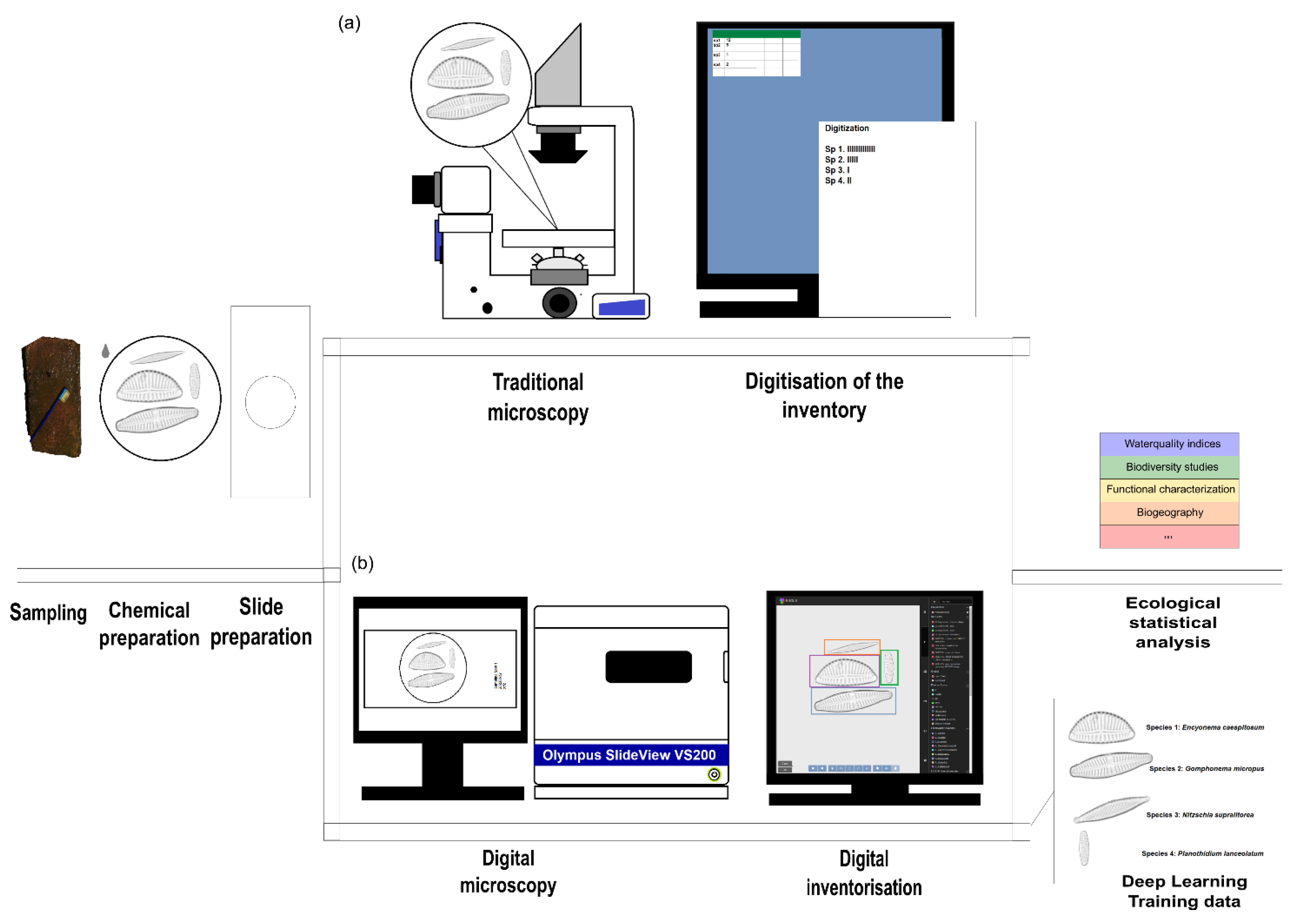
2.2. “Traditional” Diatom Identification Workflow

The slides were screened using a Zeiss Axio Vert.A1 (Carl Zeiss AG, Oberkochen, Germany) light microscope with an N-Achroplan 100×/1.25 oil immersion objective. When deemed necessary for identification, basic morphometric features (length, width, striae density) were measured after capturing a digital image with the Zen software v. 3.5 (Carl Zeiss AG, Oberkochen, Germany) using an AxioCam 305 color camera (Carl Zeiss AG, Oberkochen, Germany). 400 diatom valves within the previously selected slide section were identified and counted by taxon following a standard serpentine pattern. Diatom valves crossing the right and bottom edges of the field of view were not counted to avoid repeatedly counting the same specimen.

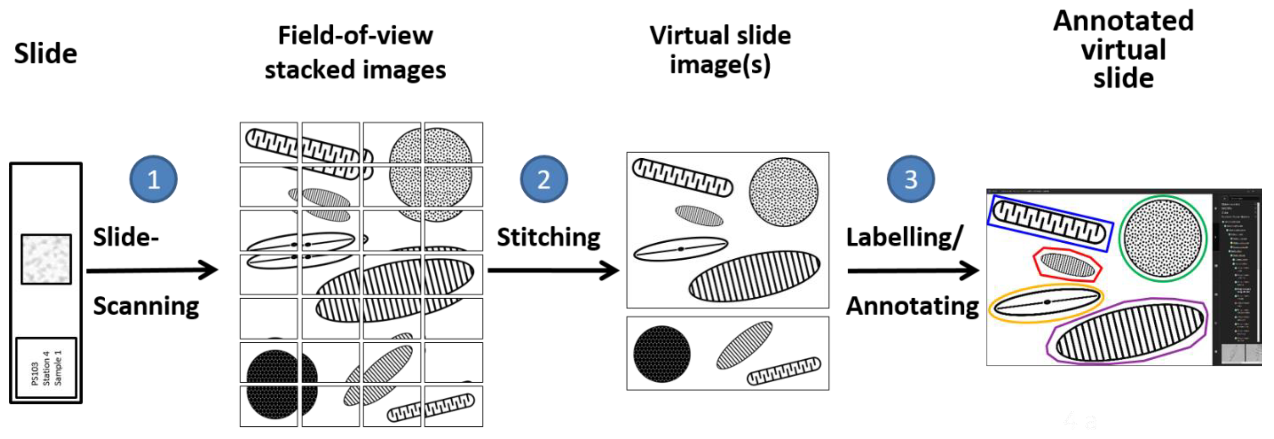
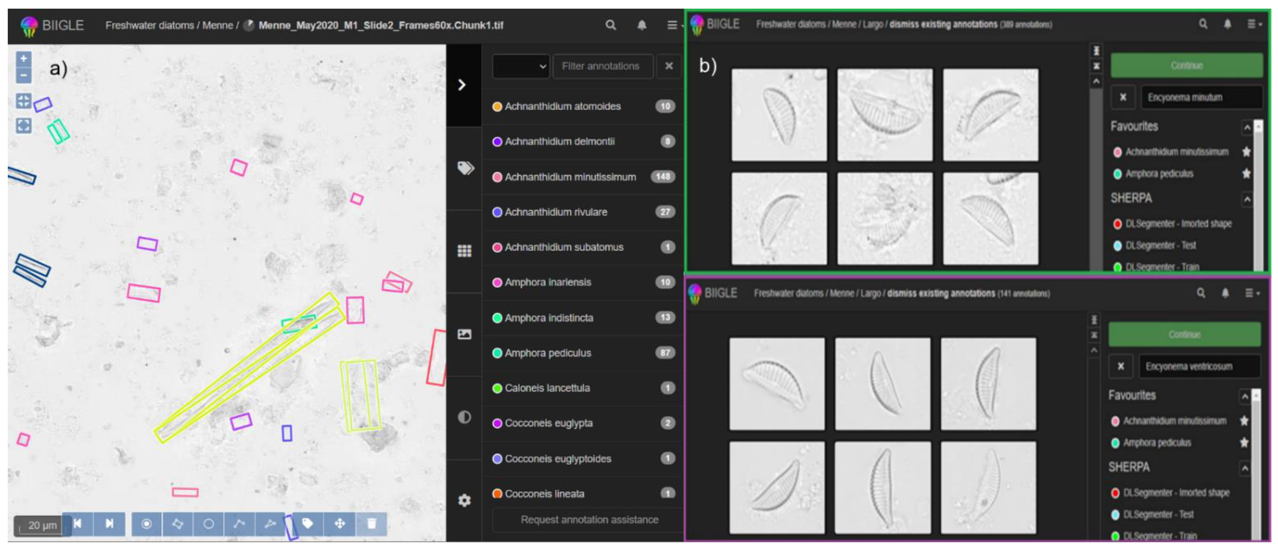
2.3. Digital Diatom Identification Workflow

In the second approach we used a digital analysis workflow, a slightly modified version of the one previously used by Burfeid-Castellanos et al. ([21], Figure 2). Slide scanning was performed with a VS200 slide scanner (Olympus Deutschland GmbH, Hamburg, Germany) with the ASW 3.1 software (Olympus Soft Imaging Solutions GmbH, Münster, Germany). The scan utilized a high-resolution oil immersion objective (UPlanXApo 60×/1.42) over a contiguous area of ca. 5 × 5 mm², which included the section of the slide that previously had been observed in the traditional workflow. For each field of view position 61 images were captured at different focus depths at a distance of 0.28 µm along the vertical Z-axis. The exact number of Z-layers required is dependent on scan area and tilt of cover slip; this number was determined to be appropriate for the set of samples considered here by trial and error. The distance between adjacent focal layers corresponds to half of the optical system’s depth of field to ensure that all ornamental valve details are captured. Neighbouring fields of view were captured with 10% overlap. The 61 images from each field of view were focus-stacked to an extended depth of field (EDF) image using the commercial Helicon Focus 7 Software (Helicon Soft Ltd., Kharkiv, Ukraine) [32], the resulting EDF image were then stitched to the final virtual slide image by combining two ImageJ plugins as described in Kloster and collaborators [33]. Each of these virtual slides had sizes of about 3 gigapixels with a single pixel depicting an area of 0.09 × 0.09 μm2 and an enhanced depth of field of 16.8 µm obtained from focus stacking. To keep the image file size below 2 gigabytes, which is a common limit for image processing software, the virtual slide images were converted to grayscale and divided into two subsections. These were uploaded into the web-based image annotation system BIIGLE 2.0 [22,34], from which point on we refer to them as “virtual slides”.
Subsequently, diatom valves were identified on each virtual slide as described below, screening the area approximately corresponding to that observed in the traditional light microscopy method. The BIIGLE 2.0 system enables flexible manual navigation across the whole sample area at arbitrary zoom/magnification levels (e.g., first screening of slide for getting an overview of taxa present; zooming in onto any individual valve for fine detail needed for identification). Systematic “row-by-row” screening of the virtual slide was performed until at least 400 diatom valves were counted, resembling the procedure applied during a traditional light microscopic count by using a function which is referred to as “Lawnmower mode” in BIIGLE. All individual diatom valves were annotated by marking their approximate outline and attaching a label corresponding to their taxonomic identification (Figure 3a). When deemed necessary for precise identification, basic morphometric features (length, width, striae density) were measured with the line measurement function of BIIGLE. Depending on the density of the diatom valves, either one or both subsections of the slide scan were required to reach the minimum of 400 valves per sample.
After all identifications were made, a quality assessment step was conducted, in order to spot misidentifications. The Label Review Grid Overview (LARGO) tool of BIIGLE was used to display side-by-side thumbnail images of all image areas (diatom valve images) annotated with a specific taxonomic label (Figure 3b). This tool facilitates synchronous observation of all valves identified as a specific taxon and enables easy recognition of morphological outliers, and so facilitates quality assessment in a way that has no analogue in the traditional microscopy workflow. For any morphological outliers or other problems spotted, it is possible to re-evaluate them in full original resolution, and to re-label them with the corrected taxon name if necessary.
The traditional vs. the digital workflow were compared by (1) community compositions; (2) diversity indices; (3) diatom indices. Since community composition determines the other two, the comparison of biotic diatom and diversity indices might be considered dispensable, nevertheless we conducted them because such comparisons are often presented in similar methodological comparisons [11,35].

2.4. Calculation of Biotic Indices

The diatom inventories obtained through the two different approaches were imported into the OMNIDIA v. 6.0.4 software [36,37] to calculate biotic diatom indices. We investigated four indices responding to nutrient concentrations (‘trophic’ indices): the Rott Trophic Index, (Rott TI, [38]); Polluosensitivity Index (IPS, [39,40]), Biological Diatom Index (IBD, [41]), the indice des diatomées génerique (IDG, [42]) and the Trophic Diatom Index (TDI, [43]). Additionally, two indices that respond to organic matter concentration (saprobic indices) were selected: Rott Saprobic Index (Rott SI, [44]) and Sládeček (SLA, [45]). All indices were calculated for each replicate of each sample separately.

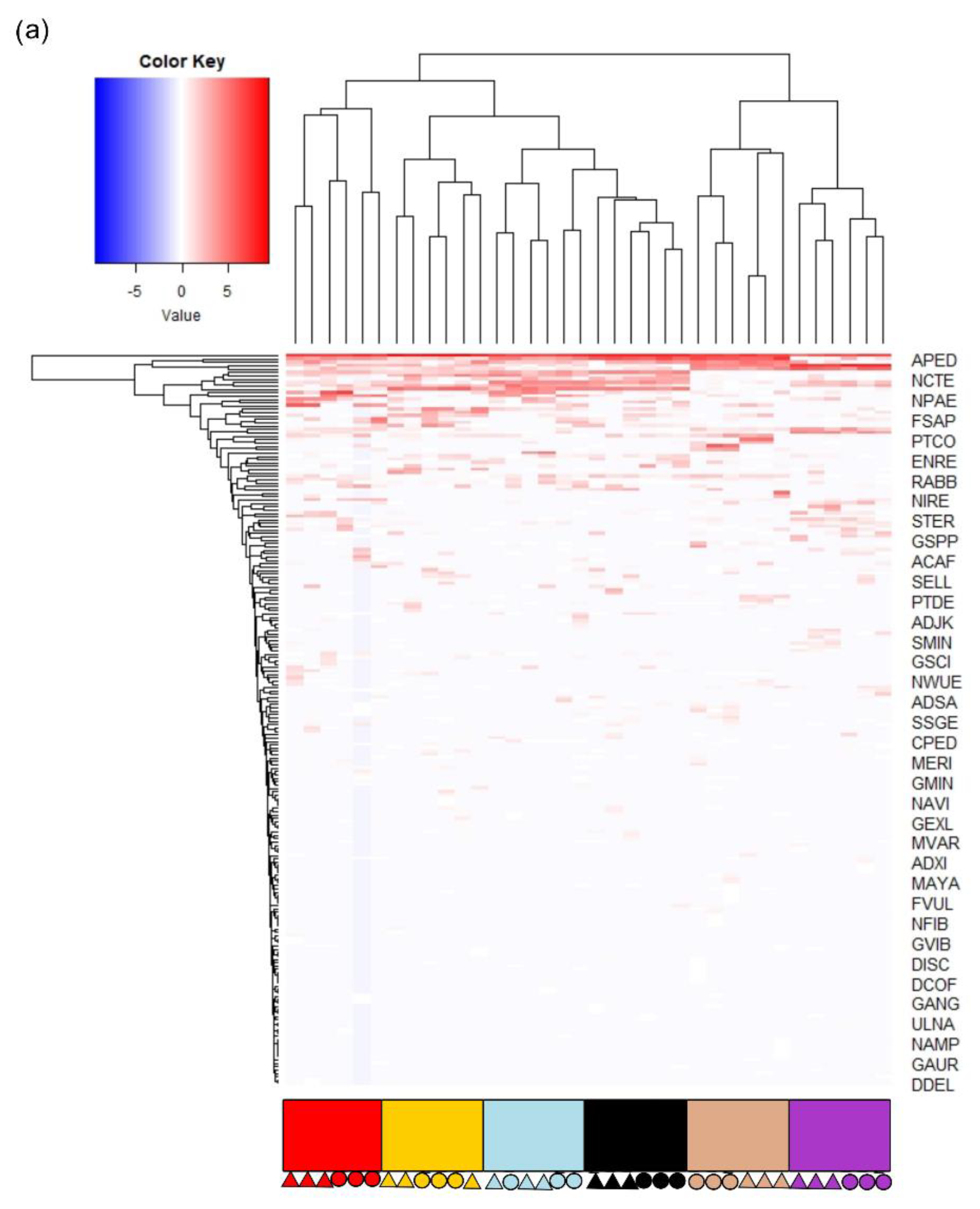
2.5. Statistical Analysis

The R software v. 3.6.1 [46] with RStudio v. 1.2.5019 [47] was used for statistical analysis. Species richness and Shannon as well as Simpson diversity metrics were calculated using the ‘vegan’ package [48].
One-way ANOVA and Kruskal-Wallis tests from the ‘R Base’ package were executed on species richness and diversity, as well as on biotic indices to test the statistical effect of the analysis method (traditional vs. digital) by sample. Tukey post-hoc tests (Tukey HSD, ‘R Base’ package) and Dunn tests (‘FSA’ package) were performed on parametric and non-parametric variables, depending on whether the outcome variable showed a significant deviation from a normal distribution as assessed by a Shapiro-Wilks-test respectively.
Relative abundances of diatoms were log-transformed for comparing community compositions as determined by the different methods. These data were used for a non-metric multidimensional scaling (nmds) and ANOSIM based on Bray-Curtis distances with the ‘vegan’ package. Effect of method (traditional vs. digital) upon observed community composition was tested by pairwise multilevel comparison of the ANOSIM results using the ‘pairwiseAdonis’ function [49].
A heatmap depicting relative abundances of predominant taxa among sampling sites was created using ‘gplots’ [50].
Besides applying the above comparative analysis to the final results, some comparisons were repeated with a transformed data set. In these cases, from taxon complexes, which are closely related and highly similar diatoms that are hard to resolve via light microscopy, individual taxa (species/varieties) were pooled at the level of the taxon complex (Table 1). The motivation behind this analysis was to test to which extent any disagreement between the traditional and digital method can be explained by varying degrees of granularity in the identification of these difficult to differentiate taxa.

3. Results & Discussion

3.1. Time Requirement

When comparing time usage for both methods, we only considered the steps of counting and preparation of abundance lists that had to be conducted by the taxonomic diatom expert. These included:
(a) Identification: In the digital microscopy workflow, diatom identification took approximately one hour longer per slide than in the traditional workflow. This additional time requirement can be explained by the fact that annotating the rough outlines of diatom valves and selecting the corresponding taxon labels takes few seconds per valve (estimating this roughly as 3600 s extra time/400 valves = ca. 9 s per valve). A second partial explanation for the extra time required in the digital workflow is that because it was simpler to measure individual valves, this also lowered the bar for measuring. Thus, probably substantially more valves were measured in the digital than in the traditional workflow, though this was not quantified.
(b) Data handling: the digital workflow did not require manual entry of inventories into a spreadsheet, as they could directly be exported from BIIGLE. In contrast, the digitization of the inventories in the traditional light microscopy method not only took some additional time, but also came at a higher risk of human error.
In total, these steps on average summed up to about 2.4 h per sample for the traditional and 3.2 h per sample for the digital approach.
On top of this, some additional tasks were conducted for the digital workflow, but are compared separately because they were either performed by technical personnel or were optional, without a corresponding step in the traditional method:
(a) An extra 15–20 min were required for setting up the scanning, downstream-processing of the digital image data and uploading the data into BIIGLE 2.0, which was performed by technical personnel. The time requirement of this step can vary depending on the exact details of the scanning procedure, including the slide scanner used, and the experience of the person conducting these steps.
(b) In the digital workflow, we implemented an additional quality assessment step that has no direct correspondence in the traditional workflow. For this, thumbnail images of all valves labelled with a user-selected taxon were evaluated side-by-side with BIIGLE’s LARGO function. Checking/confirming/revising all annotated valves/frustules took ca. 12 min per slide on average. In the traditional light microscopy approach, the full repetition of all the identification steps would be required for a similar quality assessment, due to the lack of image documentation. Since such a LARGO confirmation can be applied across a larger number of slides after all have been counted, the time requirement for this step is expected to grow slower than linear with the number of samples analysed.

3.2. Diatom Communities

A total of 161 species were identified using the digital method (number of valves [n] = 8858) and 130 species were identified using the traditional methodology (n = 9306), their distribution can be observed in Supplement Table S1. Community structures were compared using a Bray-Curtis dissimilarity matrix on log (x + 1) transformed relative abundances. The similarities ranged from 61.8% to 72.1%, with exception of the sparse sample M2 which only reached a maximal similarity of 51.6% between identical samples analysed with the digital vs. traditional workflow. Comparing communities between the traditional vs. digital counts of identical samples, ANOSIM showed no significant differences (Table 2). In a hierarchical cluster analysis of the dissimilarities of the community (Figure 4a, Supplement Figure S1), triplicates from the traditional and digital counts always clustered together. Similarly, a NMDS analysis showed a clustering of sites regardless of method (stress = 0.172, Figure 4b). Only communities from triplicates from sites M3 and M6 were intermingled in the cluster analysis, which can be explained by the high similarity between both communities. Two M2 samples analysed with the digital method did not cluster very well with other samples of the same location, which we attribute to the very low density of the sample material on these slides, which may have resulted in a smaller overlap between the areas analysed with both methods and thus might differ in species represented by only a few specimens.

3.3. Testing the Effect of Difficult Species Complexes

When comparing counts from both methods, it became apparent that taxa from some difficult species complexes were differently assessed by the two methods (Table 1) in spite of the fact that all counts were performed by the same person. To counter this, the inventories of both methods were reduced to standardize the difficult taxa. The most abundant such difficult taxon was the Achnanthidium minutissimum s.l. complex (see Table 1 for a list of taxa understood here to be part of this complex). Achnanthidium minutissimum var. jackii and Achnanthidium saprophilum were more easily discerned with the digital method, given that these very small diatoms (under 20 µm) have very slightly silicified ornamentations that were better visible in the digital extended depth of field virtual slide images.
The also monoraphid Cocconeis placentula complex (Table 1; Jahn et al. 2009; Jahn et al. 2020) was more readily identifiable by the rapheless valves, both in the traditional light microscopy and the digital method. Focus stacking in the digital method helped to recognize the raphe valve, which is mostly identifiable through morphometric features, in addition to the translucent rapheless valve. Similar was the case for the Nitzschia palea complex (Table 1). Individual taxa belonging to this complex are often identifiable by length-to-width ratio, which were more easily obtained using the digital method because it made such measurements much simpler and quicker to perform. Also, the small monoraphid Psammothidium grischunum complex (Table 1) contains many similar taxa which can appear in the same ecosystem. The taxon complex could be identified with a higher taxonomic resolution in the digital workflow due to better discrimination of morphometric and ornamentation features [56,57,58].
Specimens of the rare genera Luticola and Mayamaea, with a relative abundance under 3%, were most likely accidentally split into several species in the traditional workflow probably due to misidentification. Very rarely, specimens of the Ulnaria genus appeared, very long diatoms (>100 µm) with a taxonomy mostly based on a combination of striae density and apex form. These were assigned to multiple different species with the traditional light microscopy method, whereas identification with the digital method showed them to pertain to Ulnaria ulna. This again could point to a more precise morphometric characterization by the digital microscopy identification workflow.
A final category comprises easily overlooked taxa such as Fistulifera, a small naviculoid diatom with a very light silicification that often gets eroded during the preparation process, leaving only the raphe channel visible [54]. This taxon was slightly overrepresented in the results of the digital, compared to the traditional, method. Even though both Fistulifera saprophila and F. pelliculosa were present, they were pooled in the reduced dataset, as in the traditional light microscopy method the supposed F. pelliculosa specimens were erroneously identified as F. saprophila.
All in all, these can be interpreted as cases in which the digital method allows a more fine-grained identification, or a lower chance of overlooking hardly visible taxa (like Fistulifera) compared to the traditional analysis. To test whether such cases can explain the significant differences observed for richness at the M1 site, a “reduced” data set was obtained from the original counts by pooling taxa at the level of species complexes in the above listed cases (Table 1). Comparing richness values from the traditional vs. digital counts from site M1 showed no significant difference between both methods, nor for any other sample (Table 2, 3rd column), but the latter was expected since these showed no significant differences between richness values in the non-reduced dataset either (Table 2, 2nd column). Taxa composition and species richness within samples were not significantly different by analysis method either (Table 2, 4th column).

3.4. Biotic Indices

To further evaluate whether both methods led to comparable results, we assessed whether a range of other commonly used community metrics (Shannon diversity, Simpson diversity, trophic diatom indices IPS, IBD, IDG, TDI, Rott TI and the saprobic diatom indices Rott SI and SLA) differed between the traditional vs. digital counts of identical samples (Supplement Figure S2). In the case of all diatom indices, neither an ANOVA nor a non-parametric test showed a significant method effect after controlling for sample (Table 3). For Shannon entropy, ANOVA and Kruskal Wallis did not indicate significant differences between methods of the complete and reduced dataset. Explanation of species richness see above.

3.5. Overall Observations

In this contribution, we described how a largely digitized workflow can be used for diatom identification and counting. The traditional light microscopy method is being widely used in ecological research as well as water quality monitoring activities. This method involves the identification and counting of oxidized and mounted diatom valves/frustules using a light microscope, resulting in an inventory of counted valves per taxon. The here introduced digital workflow presents an alternative to the aforementioned traditional approach by using a modern slide-scanning microscope and web-based technologies which enable documenting every single specimen of a diatom sample as part of a virtual slide image

3.5.1. The Digital Workflow Provides Comparable Results with the “Traditional” One

The between-methods comparisons only showed significant differences in the most variable metrics, species composition and species richness, and only for a single one out of six samples. Pairwise Bray-Curtis distances between counts obtained from the same slide but with both methods varied between 0.27 and 0.382, which is a range considered to be consistent in diatom studies [13,59]. Altogether, our general first conclusion is that the digital method leads to comparable results with the traditional one.
Finding that the results were not quite identical, and significant differences were found between both methods in a single case, we hypothesized that a main explanation of differences between both methods could be explained by slight inconsistencies in the fine-grained identification of a few individual taxa in some difficult species complexes, like Achnanthidium minutissimum s.l., Cocconeis placentula s.l., Nitzschia palea s.l. (Table 1). This indeed seems to be the case, as detailed above, and is comparable to taxonomic inconsistency expectable for instance if the same analyst uses different microscopes with slightly different optics (e.g., DIC vs. bright field or phase contrast). However, our impression is that the taxonomic precision obtained with the digital method is not inferior, but in some cases, even better than in the traditional workflow. We explain this by the combination of several factors, including easier to perform morphometric measurements, often improved visibility of striation and better visibility of lightly silicified taxa like Fistulifera in extended depth of field images, and to a substantial extent by the additional quality assessment step. The latter allows to better reflect upon and reconsider individual specimen identifications after having seen the whole sample and, in some cases, to avoid an inconsistent or unwarranted species splitting based on first impressions. In this study, we had a single diatomist identifying diatoms for the methods comparison. Although this is not unusual for methodological comparisons in the diatom literature [60,61], final conclusions about intra- vs. inter-observer variability in counting results in comparison to differences arising from the digital vs. traditional workflow will need further studies with multiple experts identifying samples using both methodologies. Until such a study can be performed, research combining both types of methods will need some extra care for data collation/synthesis.
From the point of view of the human analyst identifying diatoms, a drawback of the digital workflow in its presented implementation is that, due to focus-stacking, the depth information is not preserved in the virtual slides. This means it is not possible to focus up and down through the specimen to get an idea about its three-dimensional structure, as it could be done during traditional counting. Also, identifying diatoms in focus-stacked images might require a certain adjustment from an analyst, since a specimen might look slightly different than directly on the microscope. On the other hand, focus-stacking increases the visibility of very slightly silicified structures, which often benefits taxonomic identification. Our experience shows that adjustment to extended-depth-focus is quick for a seasoned diatomist. We also note that it is not strictly necessary to limit the digital workflow to extended depth of field/focus-stacked images: the slide scanner used is also capable of obtaining virtual digital slides preserving individual focus level images. The BIIGLE 2.0 annotation platform we used, however, currently does not support such multi-depth virtual digital slides, which is a technical limitation that might be remedied in the future.

3.5.2. The Digital Workflow Is Slightly More Time Consuming, but Enables Better Scientific Practice

We found that performing a diatom count with the digital workflow took about 30% more time than with the traditional workflow. Even though annotating a diatom (marking its outline and attaching a taxonomic label to it) only took a few dozen seconds on average, this is substantially more than the handling time required in the traditional workflow, and the difference added up to about an hour over ca. 400 diatoms per sample.
Another factor contributing to the higher time-requirement of the digital workflow was the extensive use of morphometric measurements. These can be conducted much faster than in the traditional workflow, but in turn were performed much more often to help identification of hard-to-differentiate taxa. In this sense, the additional time investment translated into an increased taxonomic resolution and/or precision.
This higher time requirement can, at first sight, certainly be seen as a disadvantage of the digital method. We would argue, however, that substantial gains related to good scientific practice such as reproducibility and transparency can outweigh this disadvantage [62].
Such a taxonomically annotated virtual slide is an information-rich resource for downstream analyses. For instance, it is possible to extract counts of valves labelled with any or all taxonomic labels, as done for our comparisons; but also to extract an image cropped to the area surrounding any or all annotated valves from a virtual slide. Whereas the former represents the final (and only) output from traditional diatom counting, the latter (individual valve images) can accompany and enrich such a data set and can be used for instance for taxonomic consistency checking by human analysts, but also for image analyses aimed at morphometric characterization or taxonomic identification. Finally, in addition to sharing such data sets extracted from the virtual digital slides, it is also possible to archive and share the full virtual slide image alongside all annotations attached to it, enabling a level of transparency previously unattainable for routine diatom count data sets.
In the traditional method, every single diatom identified is generally seen only once, by one single analyst. In the case of the digital workflow, images of every single diatom encountered are available, revisitable and shareable through the internet. The additional quality assessment step we implemented above (looking at all diatoms assigned to a taxon and spotting outliers) is only one example of the multitude of ways in which this can become useful.
The digital workflow also facilitates checking for taxonomic consistency after having counted multiple slides. Especially when analysing a flora that the analyst was previously not deeply familiar with, a certain concept drift (slight changes in the way to recognize individual taxa) during a study can occur. In such cases, it can be useful to implement a quality assessment step in which any identifications can be updated, corrected and harmonized at one final time point. Such a quality assessment or consistency check could also be useful in projects where multiple analysts count subsets of samples. With the digital method, once all counts are performed, a taxonomic consistency check can be performed easily, and might even focus on particularly problematic taxa only. In the traditional workflow, comparable re-analysis would require a full re-count of all samples involved, basically starting with the whole analysis process all over again.
If taxonomically annotated images or virtual digital slides were made available routinely, similar taxonomic consistency control would also become possible beyond individual studies, for instance for larger scale data integration and synthetic analyses at large geographic scales. The problem of taxonomic consistency has long been considered an important issue for standardizing diatom-based environmental biomonitoring [63,64]. Although methods have been proposed to increase quality and reproducibility of diatom counts [15,65,66], these all rely on traditional light microscopy. As such, they do not readily enable a full transparency or re-analysis at the level of individual diatoms. If any documentation by microphotographs is involved, it is limited to a selection of one or a few examples per taxon/morphological unit. The digital method can remedy this problem by documenting each individual cell not only by its taxonomic identification but also by the corresponding image data.
We suggest that in the near future, web-based annotation of virtual digital slides in a distant collaborative setting (which was not investigated here, but is possible without further technical extensions in the introduced framework and was implemented by us for example to conduct international taxonomy workshops during the COVID pandemic) has the potential to increase the degree of taxonomic consistency substantially [13,14,15]. By hiding annotations made by other users, a feature of BIIGLE’s “annotation session” function, the agreement of independent taxonomic identifications among analysts on a common set of specimens can be quantified, and conflicts can be resolved like it was done in Beszteri et al. [14], but with less effort and as part of an integrated workflow. This way, taxonomic consistency checking can become part of routine multi-analyst counting procedures.
Finally, well-curated taxonomically annotated sets of specimen images resulting from such procedures can provide high quality data sets for training specialists in diatom identification, or also machine learning algorithms, as we demonstrated recently [34]. Computer vision/machine learning techniques have a large potential to further transform and assist the process of diatom analysis, for instance by detection of diatom valves on a virtual slide image, obviating the necessity for the human analyst to draw outline annotations, which in the here presented digital workflow is the most time consuming step [67,68,69,70,71]. Other steps which can expedite the digital variant include clustering diatom valves by their similarities to assist human annotation [17,72]; proposing taxonomic identifications based on taxon classifier models [33]; automatic digital morphometry [67,73,74]; or even by fully automated taxonomic identifications [33,72,75,76,77,78].

4. Conclusions

We propose a digital workflow combining high resolution slide scanning and web-based virtual slide annotation as a possible alternative to “traditional” light microscopic analysis of diatom community composition. In our comparison, the digital workflow provided comparable results with the traditional light microscopy, but in some cases with finer taxonomic resolution. The disadvantage is an increased time spent on measuring and labelling individual valves, which may be reduced with future informatic support. On the other hand, digital microscopy can contribute to increasing reproducibility and transparency, and provides much simpler possibilities for quality control, taxonomic updates, multi-expert collaboration or even taxonomic intercalibration. The visual appearance of diatoms in EDF (i.e., focus-stacked) images may differ from single focal plane images. However, this is relatively easy to adapt to for an experienced diatomist. A further advantage of the digital method is the by-product of annotated digital images, and the resulting labelled specimen images can be used for training machine and deep learning algorithms.

Supplementary Materials

The following supporting information can be downloaded at: https://www.mdpi.com/article/10.3390/w14203332/s1, Figure S1: Complete hierarchical clustering with triplicate annotation and complete list of diatoms using OMNIDIA 4-letter code; Figure S2: Pairwise comparison of diversity and biomonitoring indices of all samples depending on analysis method. Diversity and species values: (a) species richness, (b) Shannon diversity entropy, (c) Simpson diversity entropy. Trophic biomonitoring indices: (d) Indice de polluosensitivité (IPS), (e) Indice biologique des diatomées (IBD), (f) Trophic diatom index (TDI), (g) indice des diatomées génerique (IDG), (h) Rott Trophic index (Rott TI). Saprobic biomonitoring indices: (i) Rott saprobic index (Rott SI), (j) Sladecek saprobic index (Sladecek). Methods summarized as trad = “traditional” light microscopy and digi = digital microscopy. Video S1: Virtual diatom slide preparation process. Table S1: Species distribution along the sites. Percentage distribution on the triplicates. Methods: mic = traditional light microscopy, scan = digital microscopy. Percentages: +++ > 50%, 50% > ++ > 25%. 25% > + > 10%, 10% > r (rare) > 5%, 5% > vr (very rare) > 0.

Author Contributions

Conceptualization, A.M.B.-C., M.K. and B.B.; methodology, A.M.B.-C. and M.K.; software, M.K. and M.Z.; validation, S.B., B.B. and T.W.N.; formal analysis, B.B.; investigation, A.M.B.-C.; resources, B.B. and T.W.N.; data curation, A.M.B.-C.; writing—original draft preparation, A.M.B.-C.; writing—review and editing, A.M.B.-C., M.K., S.B., U.P., M.S., M.Z., T.W.N. and B.B.; visualization, A.M.B.-C. and M.K.; supervision, B.B. and T.W.N.; project administration, B.B.; funding acquisition, B.B. and T.W.N. All authors have read and agreed to the published version of the manuscript.

Funding

This work was partially funded under grant nrs. BE4316/7-1, BE4316/10-1 & NA 731/9-1 by the priority programme SPP 1991 Taxon-OMICS of the Deutsche Forschungsgemeinschaft (DFG). MZ was supported by BMBF project COSEMIO (FKZ 03F0812C). This work was supported by the BMBF-funded de.NBI Cloud within the German Network for Bioinformatics Infrastructure (de.NBI) (031A532B, 031A533A, 031A533B, 031A534A, 031A535A, 031A537A, 031A537B, 031A537C, 031A537D, 031A538A).

Institutional Review Board Statement

Not applicable.

Informed Consent Statement

Not applicable.

Data Availability Statement

All data and R scripts used for this article are open access and are available at Zenodo (https://doi.org/10.5281/zenodo.5517381), the digital slide scans and annotations can be viewed online in BIIGLE (direct link: https://biigle.de/images/1933537/annotations?scaleLine=1&zoomLevel=1&labelTooltip=1 (accessed on 3 March 2022), login: “[email protected]”, password: “microscopy”). A video summary of the digital workflow can also be found here (https://zenodo.org/record/7227922 (https://doi.org/10.5281/zenodo.7227922, accessed on 20 October 2022)).

Acknowledgments

We would like to thank Kreis Paderborn for permits for sampling in the Menne catchment.

Conflicts of Interest

The authors declare no conflict of interest.

References

  1. Lama, G.F.C.; Errico, A.; Pasquino, V.; Mirzaei, S.; Preti, F.; Chirico, G.B. Velocity uncertainty quantification based on Riparian vegetation indices in open channels colonized by Phragmites australis. J. Ecohydraulics 2022, 7, 71–76. [Google Scholar] [CrossRef]
  2. Jalonen, J.; Järvelä, J.; Koivusalo, H.; Hyyppä, H. Deriving Floodplain Topography and Vegetation Characteristics for Hydraulic Engineering Applications by Means of Terrestrial Laser Scanning. J. Hydraul. Eng. 2014, 140, 4014056. [Google Scholar] [CrossRef]
  3. Lowe, R.L. Environmental Requirements and Pollution Tolerance of Freshwater Diatoms EPA-670/4-74-005; National Environmental Research Center Office of Research and Development, U.S. Environmental Protection Agency: Cincinnati, OH, USA, 1974. [Google Scholar]
  4. Patrick, R. The Importance of Monitoring Change. In Biological Monitoring of Water and Effluent Quality; Cairns, J., Dikinson, K.L., Westlake, G., Eds.; American Society for Testing and Materials: West Conshohocken, PA, USA, 1976; pp. 157–190. [Google Scholar]
  5. Falasco, E.; Bona, F.; Monauni, C.; Zeni, A.; Piano, E. Environmental and spatial factors drive diatom species distribution in Alpine streams: Implications for biomonitoring. Ecol. Indic. 2019, 106, 105441. [Google Scholar] [CrossRef] [Green Version]
  6. Ehrenberg, C.G. Die Infusionsthierchen als Vollkommene Organismen; Leopold Voss: Leipzig, Germany, 1838. [Google Scholar]
  7. Lobo, E.A.; Heinrich, C.G.; Schuch, M.; Wetzel, C.E.; Ector, L. Chapter 11. Diatoms as Bioindicators in Rivers Eduardo A. Lobo, Carla Giselda Heinrich, Marilia Schuch, Carlos Eduardo Wetzel, and Luc Ector. In River Algae; Necchi, O., Ed.; Springer: Cham, Switzerland, 2016; ISBN 978-3-319-31983-4. [Google Scholar]
  8. Smol, J.P.; Stoermer, E.F. (Eds.) The Diatoms: Applications for the Environmental and Earth Sciences, 2nd ed.; Cambridge University Press: Cambridge, UK, 2012; ISBN 978-1-107-56496-1. [Google Scholar]
  9. Morales, E.A.; Siver, P.A.; Trainor, F.R. Identification of diatoms (Bacillariophyceae) during ecological assessments: Comparison between Light Microscopy and Scanning Electron Microscopy techniques. Analysis 2001, 151, 95–103. [Google Scholar] [CrossRef]
  10. Pérez-Burillo, J.; Trobajo, R.; Vasselon, V.; Rimet, F.; Bouchez, A.; Mann, D.G. Evaluation and sensitivity analysis of diatom DNA metabarcoding for WFD bioassessment of Mediterranean rivers. Sci. Total Environ. 2020, 727, 138445. [Google Scholar] [CrossRef]
  11. Bailet, B.; Bouchez, A.; Franc, A.; Frigerio, J.-M.; Keck, F.; Karjalainen, S.-M.; Rimet, F.; Schneider, S.; Kahlert, M. Molecular versus morphological data for benthic diatoms biomonitoring in Northern Europe freshwater and consequences for ecological status. Metabarcoding Metagenomics 2019, 3, e34002. [Google Scholar] [CrossRef] [Green Version]
  12. Borrego-Ramos, M.; Bécares, E.; García, P.; Nistal, A.; Blanco, S. Epiphytic Diatom-Based Biomonitoring in Mediterranean Ponds: Traditional Microscopy versus Metabarcoding Approaches. Water 2021, 13, 1351. [Google Scholar] [CrossRef]
  13. Kahlert, M.; Ács, É.; Almeida, S.F.P.; Blanco, S.; Dressler, M.; Ector, L.; Karjalainen, S.M.; Liess, A.; Mertens, A.; van der Wal, J.; et al. Quality assurance of diatom counts in Europe: Towards harmonized datasets. Hydrobiologia 2016, 772, 1–14. [Google Scholar] [CrossRef] [Green Version]
  14. Beszteri, B.; Allen, C.; Almandoz, G.O.; Armand, L.; Bárcena, M.A.; Cantzler, H.; Crosta, X.; Esper, O.; Jordan, R.W.; Kauer, G.; et al. Quantitative comparison of taxa and taxon concepts in the diatom genus Fragilariopsis a case study on using slide scanning multiexpert image annotation and image analysis in taxonomy. J. Phycol. 2018, 54, 705–719. [Google Scholar] [CrossRef] [Green Version]
  15. Tyree, M.A.; Bishop, I.W.; Hawkins, C.P.; Mitchell, R.; Spaulding, S.A. Reduction of taxonomic bias in diatom species data. Limnol. Oceanogr. Methods 2020, 18, 271–279. [Google Scholar] [CrossRef]
  16. Kloster, M.; Esper, O.; Kauer, G.; Beszteri, B. Large-Scale Permanent Slide Imaging and Image Analysis for Diatom Morphometrics. Appl. Sci. 2017, 7, 330. [Google Scholar] [CrossRef] [Green Version]
  17. Cristóbal, G.; Blanco, S.; Bueno, G. (Eds.) Modern Trends in Diatom Identification; Springer International Publishing: Cham, Switzerland, 2020; ISBN 978-3-030-39211-6. [Google Scholar]
  18. Du Buf, J.M.H.; Bayer, M.M. (Eds.) Automatic Diatom Identification (ADIAC); World Scientific Publishing Co. Pte. Ltd.: London, UK, 2002; ISBN 978-85-7811-079-6. [Google Scholar]
  19. Pinto, R.; Vilarinho, R.; Carvalho, A.P.; Moreira, J.A.; Guimarães, L.; Oliva-Teles, L. Novel Approach to Freshwater Diatom Profiling and Identification Using Raman Spectroscopy and Chemometric Analysis. Water 2022, 14, 2116. [Google Scholar] [CrossRef]
  20. Burfeid-Castellanos, A.M.; Kloster, M.; Cambra, J.; Beszteri, B. Both hydrology and physicochemistry influence diatom morphometry. Diatom Res. 2020, 35, 1–12. [Google Scholar] [CrossRef]
  21. Burfeid Castellanos, A.M.; Martín-Martín, R.P.; Kloster, M.; Angulo-Preckler, C.; Avila, C.; Beszteri, B.; Burfeid-Castellanos, A.M.; Kloster, M.; Angulo-Preckler, C.; Beszteri, B. Epiphytic diatom community structure and richness is determined by macroalgal host and location in the South Shetland Islands (Antarctica). PLoS ONE 2021, 16, e0250629. [Google Scholar] [CrossRef]
  22. Langenkämper, D.; Zurowietz, M.; Schoening, T.; Nattkemper, T.W. BIIGLE 2.0—Browsing and Annotating Large Marine Image Collections. Front. Mar. Sci. 2017, 4, 83. [Google Scholar] [CrossRef] [Green Version]
  23. Zurowietz, M.; Nattkemper, T.W. Current Trends and Future Directions of Large Scale Image and Video Annotation: Observations From Four Years of BIIGLE 2.0. Front. Mar. Sci. 2021, 8, 1752. [Google Scholar] [CrossRef]
  24. CEN. UNE-EN 13946:2014; Water Quality—Guidance for the Routine Sampling and Preparation of Benthic Diatoms from Rivers and Lakes. CEN-CENELEC Management Centre: Brussels, Belgium, 2014.
  25. CEN. UNE-EN 14407:2014; Water Quality—Guidance Standard for the Identification, Enumeration and Interpretation of Benthic Diatom Samples from rivers and lakes. CEN-CENELEC Management Centre: Brussels, Belgium, 2014.
  26. Taylor, J.C.; Harding, W.R.; Archibald, C.G.M. A Methods Manual for the Collection, Preparation and Analysis of Diatom Samples Version 1.0; TT 281/07; Water Research Commission: Pretoria, South Africa, 2007; ISBN 1-77005-483-9. [Google Scholar]
  27. Bey, M.-Y.; Ector, L. Atlas des Diatomées des Cours d’eau de la Région Rhône-Alpes; Tomes 1–6; Direction régionale de l'environnement, de l'aménagement et du logement, Préfet de la Région Auvergne-Rhône-Alpes: Lyon, France, 2013; ISBN 978-2-11-129817-0. [Google Scholar]
  28. Cantonati, M.; Hoffmann, G.; Kelly, M.G.; Lange-Bertalot, H.; Werum, M. Freshwater Benthic Diatoms of Central Europe: Over 800 Common Species Used in Ecological Assessment; Koeltz Botanical Books: Schmitten-Oberreifenberg, Germany, 2017; ISBN 978-3-946583-06-6. [Google Scholar]
  29. Bahls, L.L.; Edlund, M.B.; Kociolek, J.P.; Lowe, R.L.; Potapova, M.G.; Spaulding, S.A.; Bishop, I.; Burge, D.R.L.; English, J.; Furey, P.; et al. Diatoms of North America. Available online: https://diatoms.org/ (accessed on 30 June 2020).
  30. Levkov, Z.; Metzeltin, D.; Pavlov, A. Luticola and Luticolopsis. In Diatoms of the European Inland Waters and Comparable Habitats, 1st ed.; Bertalot, H.L., Ed.; Koeltz Botanical Books: Oberreifenberg, Germany, 2013; p. 698. ISBN 978-3-87429-439-3. [Google Scholar]
  31. Trobajo, R.; Rovira, L.; Ector, L.; Wetzel, C.E.; Kelly, M.G.; Mann, D.G. Morphology and identity of some ecologically important small Nitzschia species. Diatom Res. 2013, 28, 37–59. [Google Scholar] [CrossRef]
  32. Helicon Focus; Helicon Soft Ltd.: Kharkiv, Ukraine, 2020.
  33. Kloster, M.; Langenkämper, D.; Zurowietz, M.; Beszteri, B.; Nattkemper, T.W. Deep learning-based diatom taxonomy on virtual slides. Sci. Rep. 2020, 10, 14416. [Google Scholar] [CrossRef]
  34. Schoening, T.; Osterloff, J.; Nattkemper, T.W. RecoMIA—Recommendations for Marine Image Annotation: Lessons Learned and Future Directions. Front. Mar. Sci. 2016, 3, 59. [Google Scholar] [CrossRef] [Green Version]
  35. Bailet, B.; Apothéloz-Perret-Gentil, L.; Baričević, A.; Chonova, T.; Franc, A.; Frigerio, J.-M.; Kelly, M.; Mora, D.; Pfannkuchen, M.; Proft, S.; et al. Diatom DNA metabarcoding for ecological assessment: Comparison among bioinformatics pipelines used in six European countries reveals the need for standardization. Sci. Total Environ. 2020, 745, 140948. [Google Scholar] [CrossRef]
  36. Lecointe, C.; Coste, M.; Prygiel, J. “Omnidia”: Software for taxonomy, calculation of diatom indices and inventories management. Hydrobiologia 1993, 269, 509–513. [Google Scholar] [CrossRef]
  37. Lecointe, C.; Coste, M. Omnidia. 2015. Available online: https://omnidia.fr/en/ (accessed on 11 May 2020).
  38. Rott, E. Indikationslisten für Aufwuchsalgen in Österreichischen Fließgewässern. 2. Trophieindikation sowie geochemische Präferenz: Taxonomische und Toxikologische Anmerkungen; Bundesministerium f. Land- u. Forstwirtschaft: Wien, Austria, 1999. [Google Scholar]
  39. Descy, J.P.; Coste, M. Utilisation des diatomeés benthiques pour la mesure de la qualité des eaux du bassin Artois-Picardie: Bilan et perspectives. Ann. De Limnol. Int. J. Limnol. 1990, 29, 255–267. [Google Scholar]
  40. Prygiel, J.; Leveque, L.; Iserentant, R. Un nouvel indice Diatomique Pratique por l’évaluation de la qualité des eaux en réseau de surveillance. Rev. Des Sci. De L’Eau 1996, 1, 97–113. [Google Scholar]
  41. Prygiel, J.; Carpentier, P.; Almeida, S.F.P.; Coste, M.; Druart, J.-C.; Ector, L.; Guillard, D.; Honoré, M.-A.; Iserentant, R.; Ledeganck, P.; et al. Determination of the biological diatom index (IBD NF T 90–354): Results of an intercomparison exercise. J. Appl. Phycol. 2002, 14, 27–40. [Google Scholar] [CrossRef]
  42. Corse, P.B. Cemagref. Etude des Méthodes Biologiques Quantitatives D’appréciation de la Qualité des Eaux. Rapport Division Qualité des Eaux Lyon. 1982. Available online: https://www.documentation.eauetbiodiversite.fr/notice/00000000015def9cd65cdb328423f073 (accessed on 2 January 2019).
  43. Kelly, M.G.; Whitton, B.A. The trophic diatom index: A new index for monitoring eutrophication in rivers. J. Appl. Phycol. 1995, 7, 433–444. [Google Scholar] [CrossRef]
  44. Rott, E.; Hofmann, P.G.; Pall, K.; Pfister, P.; Pipp, E. Indikationslisten für Aufwuchsalgen in Österreichischen Fliessgewässern, Teil 1: Saprobielle Indikation; Bundesministerium f. Land- u. Forstwirtschaft: Wien, Austria, 1997. [Google Scholar]
  45. Sládeček, V. Diatoms as indicators of organic pollution. Acta Hydrochim. Et Hydrobiol. 1986, 14, 555–566. [Google Scholar] [CrossRef]
  46. R Development Core Team. R: A Language and Environment for Statistical Computing; R Foundation for Statistical Computing: Vienna, Austria, 2008; ISBN 3-900051-07-0. [Google Scholar]
  47. RStudio Team. RStudio: Integrated Development for R; RStudio, Inc.: Boston, MA, USA, 2015. [Google Scholar]
  48. Oksanen, J. Multivariate Analysis of Ecological Communities in R. Ph.D. Thesis, University of Oulu, Oulu, Finland, 2013. [Google Scholar]
  49. Martinez Arbizu, P. pairwiseAdonis: Pairwise Multilevel Comparison Using Adonis. 2020. Available online: https://github.com/pmartinezarbizu/pairwiseAdonis (accessed on 1 March 2020).
  50. Warnes, G.R.; Bolker, B.; Bonebakker, L.; Huber, W.; Liaw, A.; Lumley, T.; Magnusson, A.; Moeller, S.; Schwartz, M. Package ‘gplots’. 2015. Available online: https://cran.r-project.org/web/packages/gplots/gplots.pdf (accessed on 20 May 2018).
  51. Wojtal, A.Z.; Ector, L.; van de Vijver, B.; Morales, E.A.; Blanco, S.; Piatek, J.; Smieja, A. The Achnanthidium minutissimum complex (Bacillariophyceae ) in southern Poland. Algol. Stud. 2011, 136–137, 211–238. [Google Scholar] [CrossRef]
  52. Jahn, R.; Kusber, W.-H.; Romero, O.E. Cocconeis pediculus Ehrenberg and C. placentula Ehrenberg var. placentula (Bacillariophyta): Typification and taxonomy. Fottea 2009, 9, 275–288. [Google Scholar] [CrossRef]
  53. Zgrundo, A.; Lemke, P.; Pniewski, F.; Cox, E.J.; Latała, A. Morphological and molecular phylogenetic studies on Fistulifera saprophila. Diatom Res. 2013, 28, 431–443. [Google Scholar] [CrossRef]
  54. Trobajo, R.; Clavero, E.; Chepurnov, V.A.; Sabbe, K.; Mann, D.G.; Ishihara, S.; Cox, E.J. Morphological, genetic and mating diversity within the widespread bioindicator Nitzschia palea (Bacillariophyceae). Phycologia 2009, 48, 443–459. [Google Scholar] [CrossRef]
  55. Williams, D.M. Synedra, Ulnaria: Definitions and descriptions—A partial resolution. Diatom Res. 2011, 26, 149–153. [Google Scholar] [CrossRef]
  56. Novais, M.H.; Jüttner, I.; de van Vijver, B.; Morais, M.M.; Hoffmann, L.; Ector, L. Morphological variability within the Achnanthidium minutissimum species complex (Bacillariophyta): Comparison between the type material of Achnanthes minutissima and related taxa, and new freshwater Achnanthidium species from Portugal. Phytotaxa 2015, 224, 101–139. [Google Scholar] [CrossRef]
  57. Pinseel, E.; Vanormelingen, P.; Hamilton, P.B.; Vyverman, W.; de van Vijver, B.; Kopalova, K. Molecular and morphological characterization of the Achnanthidium minutissimum complex (Bacillariophyta) in Petuniabukta (Spitsbergen, High Arctic) including the description of A. digitatum sp. nov. Eur. J. Phycol. 2017, 52, 264–280. [Google Scholar] [CrossRef]
  58. Wetzel, C.E.; Jüttner, I.; Gurung, S.; Ector, L. Analysis of the type material of Achnanthes minutissima var. macrocephala (Bacillariophyta) and description of two new small capitate Achnanthidium species from Europe and the Himalaya. Plant Ecol. Evol. 2019, 152, 340–350. [Google Scholar] [CrossRef]
  59. Kelly, M.G. Use of similarity measures for quality control of benthic diatom samples. Water Res. 2001, 35, 2784–2788. [Google Scholar] [CrossRef]
  60. ter Braak, C.J.F.; van Dam, H. Inferring pH from diatoms: A comparison of old and new calibration methods. Hydrobiologia 1989, 178, 209–223. [Google Scholar] [CrossRef]
  61. Hamsher, S.E.; LeGresley, M.M.; Martin, J.L.; Saunders, G.W. A comparison of morphological and molecular-based surveys to estimate the species richness of Chaetoceros and Thalassiosira (bacillariophyta), in the Bay of Fundy. PLoS ONE 2013, 8, e73521. [Google Scholar] [CrossRef] [Green Version]
  62. Lowndes, J.S.S.; Best, B.D.; Scarborough, C.; Afflerbach, J.C.; Frazier, M.R.; O'Hara, C.C.; Jiang, N.; Halpern, B.S. Our path to better science in less time using open data science tools. Nat. Ecol. Evol. 2017, 1, 160. [Google Scholar] [CrossRef] [Green Version]
  63. Kahlert, M.; Kelly, M.G.; Albert, R.-L.; Almeida, S.F.P.; Bešta, T.; Blanco, S.; Coste, M.; Denys, L.; Ector, L.; Fránková, M.; et al. Identification versus counting protocols as sources of uncertainty in diatom-based ecological status assessments. Hydrobiologia 2012, 695, 109–124. [Google Scholar] [CrossRef]
  64. Kahlert, M.; Kelly, M.G.; Mann, D.G.; Rimet, F.; Sato, S.; Bouchez, A.; Keck, F. Connecting the morphological and molecular species concepts to facilitate species identification within the genus Fragilaria (Bacillariophyta). J. Phycol. 2019, 55, 948–970. [Google Scholar] [CrossRef]
  65. Bishop, I.W.; Esposito, R.M.; Tyree, M.; Spaulding, S.A.; BISHOP, I.W. A diatom voucher flora from selected southeast rivers (USA). Phytotaxa 2017, 332, 101. [Google Scholar] [CrossRef] [Green Version]
  66. Lee, S.S.; Bishop, I.W.; Spaulding, S.A.; Mitchell, R.M.; Yuan, L.L. Taxonomic harmonization may reveal a stronger association between diatom assemblages and total phosphorus in large datasets. Ecol. Indic. 2019, 102, 166–174. [Google Scholar] [CrossRef]
  67. Kloster, M.; Kauer, G.; Beszteri, B. SHERPA: An image segmentation and outline feature extraction tool for diatoms and other objects. BMC Bioinform. 2014, 15, 218. [Google Scholar] [CrossRef]
  68. Rojas Camacho, O.; Forero, M.G.; Menéndez, J.M.; Forero, M.; Menéndez, J. A Tuning Method for Diatom Segmentation Techniques. Appl. Sci. 2017, 7, 762. [Google Scholar] [CrossRef]
  69. Libreros, J.; Bueno, G.; Trujillo, M.; Ospina, M. Diatom Segmentation in Water Resources. In Advances in Computing, Proceedings of the 13th Colombian conference, CCC 2018, Cartagena, Colombia, 26–28 September 2018; Jairo, E., Serrano, C., Martínez-Santos, J.C., Eds.; Springer: Cham, Switzerland, 2018; pp. 83–97. ISBN 978-3-319-98998-3. [Google Scholar]
  70. Ivanova, M.V.; Vuntesmeri, Y.V.; Bukhtiiarova, L.M. Automated Detection and Classification of the Diatom Microscopic Photo Images. Mìkrosist. Elektron. Akust. 2019, 24, 18–25. [Google Scholar] [CrossRef]
  71. Fischer, S.; Shahbazkia, H.; Bunke, H. Contour Extraction. In Automatic Diatom Identification (ADIAC); Du Buf, J.M.H., Bayer, M.M., Eds.; World Scientific Publishing Co Pte Ltd.: London, UK, 2002; pp. 93–108. ISBN 978-85-7811-079-6. [Google Scholar]
  72. Westenberg, M.A.; Roerdink, J. Mixed-Method Identifications. In Automatic Diatom Identification (ADIAC); Du Buf, J.M.H., Bayer, M.M., Eds.; World Scientific Publishing Co Pte Ltd.: London, UK, 2002; pp. 245–258. ISBN 978-85-7811-079-6. [Google Scholar]
  73. Spaulding, S.A.; Jewson, D.H.; Bixby, R.J.; Nelson, H.; McKnight, D.M. Automated measurement of diatom size. Limnol. Oceanogr. Methods 2012, 10, 882–890. [Google Scholar] [CrossRef]
  74. Glemser, B.; Kloster, M.; Esper, O.; Eggers, S.L.; Kauer, G.; Beszteri, B. Biogeographic differentiation between two morphotypes of the Southern Ocean diatom Fragilariopsis kerguelensis. Polar Biol. 2019, 42, 1369–1376. [Google Scholar] [CrossRef] [Green Version]
  75. Jalba, A.C.; Wilkinson, M.H.F.; Roerdink, J.B.T.M. Automatic segmentation of diatom images for classification. Microsc. Res. Tech. 2004, 65, 72–85. [Google Scholar] [CrossRef] [Green Version]
  76. Bueno, G.; Deniz, O.; Pedraza, A.; Ruiz-Santaquiteria, J.; Salido, J.; Cristóbal, G.; Borrego-Ramos, M.; Blanco, S. Automated Diatom Classification (Part A): Handcrafted Feature Approaches. Appl. Sci. 2017, 7, 753. [Google Scholar] [CrossRef] [Green Version]
  77. Pedraza, A.; Bueno, G.; Deniz, O.; Cristóbal, G.; Blanco, S.; Borrego-Ramos, M. Automated Diatom Classification (Part B): A Deep Learning Approach. Appl. Sci. 2017, 7, 460. [Google Scholar] [CrossRef] [Green Version]
  78. Abdullah; Ali, S.; Khan, Z.; Hussain, A.; Athar, A.; Kim, H.-C. Computer Vision Based Deep Learning Approach for the Detection and Classification of Algae Species Using Microscopic Images. Water 2022, 14, 2219. [Google Scholar] [CrossRef]
Figure 1. Comparison of the methods used for diatom identification and counting. Note that the identical slides were used for the “traditional” light microscopy path (a) as well as for the digital slide scanning methodology (b). Samples were collected following UNE EN 13946 (2014), then chemically prepared, dripped onto coverslips and mounted on a slide. (a) A square subsection of the slide with the highest density of evenly distributed valves was observed under the microscope, diatoms were identified and counted. (b) approximately the same slide area was scanned using the slide scanner, leading to a virtual slide image which was uploaded to BIIGLE 2.0 for taxonomically labelling individual diatom valves within a web browser. The resulting inventories (taxa-by-sample matrices) were used to compare results from both methods.
Water 14 03332 g001
Figure 2. Construction of a virtual slide image. The slide is imaged by a slide scanning microscope, each field of view is captured at multiple focus depths that are then focus-stacked in an intermediate step (1). The focus-stacked, slightly overlapping field of view images are joined via a stitching procedure into a single, large image file encompassing the whole scanned slide area at full original resolution (2). The virtual slide images are uploaded to the BIIGLE 2.0 image annotation platform and diatoms are identified and labelled manually through a web browser, detail in Figure 3a (3). Image modified from Kloster et al. 2020 [33].
Water 14 03332 g002
Figure 3. Examples of BIIGLE functions: (a) completely identified sample with identification labels, each frustule/valve and label can be revisited if necessary e.g., for quality control. (b) LARGO function comparing morphologically similar species of the Encyonema genus for possible taxonomical updates.
Water 14 03332 g003
Figure 4. Diatom species composition [log (relative abundance + 1)] and sites (a) using a hierarchical cluster analysis, and (b) ordination by non-metric multidimensional scaling. Triplicates of the same sample cluster together, without a separation by counting method, only counts obtained from sample M2 (red) using digital microscopy show a wider spread. Four letter code explained in Supplement Table S1.
Water 14 03332 g004aWater 14 03332 g004b
Table 1. Rationale for the reduced dataset.
Combined Name/ComplexSpecies in Complete DatasetRationale
Achnanthidium minutissimum (Kützing) Czarnecki complexAchnanthidium alteragracillimum Round & BukhtiyarovaRelative similarity of the valves may bring over-specification of diatoms and enhance error [51]
Achnanthidium affine (Grunow) Czarnecki
Achnanthidium minussimum (Kützing) Czarnecki
Achnanthidium minutissimum var. jackii (Rabenhorst) Lange-Bertalot
Achnanthidium saprophilum (Kobayashi & Mayama) Round & Bukhtiyarova
Cocconeis placentula EhrenbergCocconeis placentula var. euglypta EhrenbergFollowing diatoms.org, we selected this as a complex [52]
Cocconeis placentula var. euglyptoides (Geitler) Lange-Bertalot
Cocconeis placentula Ehrenberg
Cocconeis lineata Ehrenberg
Fistulifera saprophila (Lange-Bertalot & Bonik) Lange-BertalotFistulifera saprophila (Lange-Bertalot & Bonik) Lange-BertalotTaxa difficult to differentiate with the “traditional” method [53], pooled into F. saprophila.
Fistulifera pellucida (Kützing) Lange-Bertalot
Luticola mutica (Kützing) D.G. MannLuticola goeppertiana (Bleisch) D.G. Mann ex J. Rarick, S. Wu, S.S. Lee & EdlundExpected misidentification in “traditional” method [30]
Luticola mutica (Kützing) D.G. Mann
Luticola saprophila Levkov, Metzeltin & A. Pavlov
Mayamaea atomus (Kützing) Lange-BertalotMayamaea atomus (Kützing) Lange-BertalotPossible species splitting in “traditional” method [28]
Mayamaea atomus var. alcimonica (E.Reichardt) E.Reichardt
Mayamaea atomus var. permitis (Hustedt) Lange-Bertalot
Nitzschia palea (Kützing) W. SmithNitzschia palea var. debilis (Kützing) GrunowPossible species splitting in “traditional” method [54]
Nitzschia palea (Kützing) W. Smith
Psammothidium grischunum Bukhtiyarova & RoundPsammothidium bioretii (H.Germain) Buhtiyarova & RoundPossible species splitting in “traditional” method [28]
Psammothidium daonense (Lange-Bertalot) Lange-Bertalot
Psammothidium grischunum Bukhtiyarova & Round
Ulnaria ulna (Nitzsch) CompèreUlnaria acus (Kützing) AboalPossible species splitting in “traditional” method [55]
Ulnaria danica (Kützing) Compère & Bukhtiyarova
Ulnaria (Kützing) Compère
Ulnaria ulna (Nitzsch) Compère
Table 2. Post-hoc Tukey HSD analysis to test the intra-site variation of species richness community structure according to method on the complete and the reduced dataset. In bold, significant values.
F-Value Richness Complete DatasetF-Value Richness Reduced DatasetF-Value Community Structure Reduced Dataset
M1 per method14.333 *,1−3.333 n.s.3.890 n.s.
M2 per method6.667 n.s.0.667 n.s.5.004 n.s.
M3 per method8.333 n.s.−9.000 n.s.3.927 n.s.
M4 per method10.000 n.s.−9.667 n.s.3.528 n.s.
M5 per method4.000 n.s.0.333 n.s.1.834 n.s.
M6 per method6.000 n.s.−2.333 n.s.1.695 n.s.
Note: 1 p-value: n.s. > 0.1, * p-value ≤ 0.05.
Table 3. Analysis of variance results of the parametric values. Interactions calculated only if methods were significantly different. In bold, significant values.
Type of IndicesVariables (-Test)F-Value Method
Species richness and diversity functionsSpecies richness27.66 ***,1
Shannon entropy +0.604 n.s.
Shannon–Kruskal Wallis0.025 n.s.
Simpson entropy +2.855 n.s.
Simpson–Kruskal Wallis0.169 n.s.
Trophic diatom indicesIPS0.478 n.s.
IDG0.387 n.s.
IBD0.004 n.s.
TDI0.095 n.s.
Rott TI1.479 n.s.
Saprobic diatom indicesRott SI0.066 n.s.
Sládeček0.016 n.s.
Note: 1 p-value: n.s. > 0.1, *** p-value ≤ 0.001. + = non-parametric variables warrant non-parametric test.
Publisher’s Note: MDPI stays neutral with regard to jurisdictional claims in published maps and institutional affiliations.

