Article

Monitoring Ice Phenology in Lake Wetlands Based on Optical Satellite Data: A Case Study of Wuliangsu Lake

1
State Key Laboratory of Coastal and Offshore Engineering, Dalian University of Technology, Dalian 116024, China
2
Finnish Meteorological Institute, 00101 Helsinki, Finland
*
Authors to whom correspondence should be addressed.
Water 2022, 14(20), 3307; https://doi.org/10.3390/w14203307
Submission received: 4 September 2022 / Revised: 27 September 2022 / Accepted: 18 October 2022 / Published: 19 October 2022
(This article belongs to the Special Issue Sea, River, Lake Ice Properties and Their Applications in Practices)

Abstract

:
It is challenging to obtain the ice phenology for a lake covered with a vast area of aquatic (shallow lake wetlands) using optical satellite data because possible clouds above the lake could contaminate the result. We developed a new method to tackle this challenge. Our target was Wuliangsu Lake, a large (330 km2) and shallow (1.6 m average depth) lake wetland in the Inner Mongolia Plateau. We used Landsat and Sentinel-2 imageries to extract the lake water boundary. The MOD09GQ/MYD09GQ dataset, having the highest spatial resolution among MODIS reflectivity products, was first selected to differentiate water and ice pixels. Then, we used the reflectivity state parameters containing cloud information in the dataset to filter out the cloud pixels. The ice phenology characteristics, such as freeze-up, break-up dates, and ice cover duration (ICD) between 2013 and 2022 were obtained. We further applied the air temperature correction technique to remove the outliers. The average of ICD in Wuliangsu Lake was about 127 ± 6 days. The freeze-up start and break-up end occurred on 17 November ± 5 days and 25 March ± 4 days, respectively. The remote sensing results agree well with the field observation, with a mean absolute error of 2 days. The algorithm can effectively remove the influence of aquatic plants and clouds on lake ice identification, thereby satisfying the needs of daily monitoring and ice phenology research in the lake wetlands.

1. Introduction

As a critical ecosystem in the world, the lake wetlands are uniquely crucial to water supply, water purification, water storage, biodiversity maintenance, and local climate adaptation. Lakes are essential to ensuring global water ecological security patterns [1,2]. Compared with tropical regions, lakes in middle and high latitudes freeze in winter. Ice serves as a critical medium for the mass and energy exchange between air and water, further maintaining the local climate and environmental stability [3,4]. Especially in arid regions, ice-covered period lakes affect local ecological and economic development and impact human activities. For example, lake freezing reduces evaporation from lakes, limits greenhouse gas production in the water bodies due to biological and chemical processes, and increases recreational activities (such as ice skating and winter swimming) [5,6,7]. Ice phenology studies in China are relatively rare and mainly focused on the Qinghai-Tibet Plateau compared to the abundant publications on boreal lakes [8,9]. While few studies on lake wetlands in the Inner Mongolia Plateau exist, they are entirely different from most of the aforementioned areas. Taking Wuliangsu Lake as an example, it has extensive aquatic plants, characteristic of a shallow lake. High incident solar radiation and low precipitation make the lake more sensitive to climate fluctuations, further affecting the ice phenology characteristics (such as ice cover duration, freeze-up start, and break-up end dates). These ice phenology data are good indicators of local climate change and can be widely employed in various climate studies [10,11].
Accurate records of lake ice phenology are essential to better understanding the relationship between climate change and the local environment. Field observations provide a certain amount of ice phenology data but have many limitations due to objective factors, such as logistical support difficulties and poor temporal continuity. In contrast, satellite remote sensing can cover much broader spatial and temporal ranges; therefore, it is used in lake ice phenology studies [12,13].
Active microwave sensors provide high spatial resolution (20–100 m). However, their lower temporal resolution (>3 days) limits their ability to monitor surface cover types of variations of lakes. For some shallow lakes with a short opening/closing period of ice cover, many errors would be introduced when extracting ice phenology dates [14]. Similarly, passive microwave sensors are characterized by high temporal resolution (mostly twice a day or better). Still, their lower spatial resolution (2–25 km) is only adapted to detecting large water bodies [15,16,17]. During pixels classification, significant errors also exist in investigating wetlands with narrow lake shoreline shapes and lush aquatic plants. In contrast, optical sensors, such as the Moderate Resolution Imaging Spectroradiometer (MODIS), are available for daily monitoring of surface cover types of lake wetland with temporal resolution (1–8 days) and spatial resolution (250–1000 m). MODIS surface reflectance products have been used to characterize lake ice phenology in harsh environments such as the Arctic and the Qinghai-Tibet Plateau [18,19,20]. Elsewhere, Williamson et al. [21] combined Sentinel-2 and Landsat-8 optical imageries to calculate the area, depth, and volume of supraglacial lakes in Greenland, and identified lakes that drain rapidly (≤ 4 days) using an automated algorithm. In addition, MODIS daily temperature products, and MODIS surface reflectance products combined with random forests have similarly demonstrated robust accuracy in lake ice phenology studies [22,23].
Although optical sensors have been successfully used to study lake evolution, their application in lake wetland ice phenology is still complicated. For example, determining the lake wetland boundary is the first difficulty because there are plenty of reeds and other aquatic plants on the lake water boundary. Although lake boundaries from databases such as HydroLAKES [24] have been widely used [13,25], it is cumbersome to manually distinguish them one by one due to the large data. Moreover, there is a significant interannual variation in the growth of reeds. A fixed lake water boundary would cause errors in the statistics of lake water areas, thereby increasing the uncertainty of pixel classification. Usually, the opening/closing period of ice cover is transient, and more pixel classification errors would miss capturing ice phenology dates. Therefore, to obtain accurate ice phenology in the wetland of a shallow lake, the influence of aquatic plants must be removed before accurately identifying the water/ice extent.
Moreover, clouds inevitably affect optical sensors, leading to the misjudgment of lake surface cover types. Tai et al. [26] used MODIS and Landsat products to calculate the ice phenology of Lake Selincuo over the past 20 years. The impact of clouds was removed by visual interpretation and culling of cloud-covered pixels, which would lose some of the pixels, leading to errors in the extracted ice phenology data.
To solve the existing problems in studying lake wetland ice phenology, this paper proposes a new algorithm. First of all, Landsat and Sentinel-2 products are used to separate the extent of aquatic plants, thus accurately extracting the lake water boundary. Secondly, we used the dynamic threshold method to cyclically extract water and ice pixels from the MODIS reflectance product to determine the optimal threshold that distinguishes water and ice. Thirdly, we combined four MODIS datasets to remove and re-fill cloud pixels. Finally, we removed outliers in the time series of water/ice coverage through air temperature correction. Wuliangsu Lake of Inner Mongolia was taken as an example in this study, the algorithm’s reliability was verified by comparison with field observations for future studies on the interaction between lake wetlands and the atmosphere, and the variations and trends of ice phenology in the Wuliangsu Lake were obtained according to the algorithm for the last ten years.

2. Study Area and Data

2.1. Study Area

Wuliangsu Lake (40°46′–41°7′ N, 108°41′–108°8′ E), located in Bayannur City, Inner Mongolia, China (Figure 1), is one of the eight major freshwater lakes in China. It is the largest lake wetland in the world at the same latitude. The lake has an elevation, total area, and water area of about 1018 m, 330 km2, and 130 km2, respectively. The water depth is 1.2–2.7 m, averaging 1.6 m. Wuliangsu Lake is a semi-dry and humid mid-temperate climate region, with an annual mean air temperature of 7.5 °C and relative humidity of 49.5% [27,28]. The ice-covered period usually lasts from mid-to-late November to late March. It is a lake of interest to climate and ecological researchers because of its typical shallow lake characteristics, lush aquatic plants, nearly 200 species of birds, and over 20 species of fish thriving there [27,29,30]. However, there is still a lack of long-term interannual variations in lake ice phenology, and this paper focuses on ice phenology from 2013 to 2022. As with Cai et al. [20], the range of each year is defined from 1 August to 30 July. For example, 2021 denotes 1 August 2020–30 July 2021.

2.2. Optical Satellite Data

2.2.1. MODIS Data

The National Aeronautics and Space Administration (NASA) carried the same MODIS sensor in the Terra and Aqua satellites launched on 18 December 1999 and 4 March 2002, respectively. The Terra and Aqua satellites crossed the equator at 10:30 am and 1:30 pm local time, respectively, resulting in different satellite altitude angles, relative azimuths, and cloudiness. The National Aeronautics and Space Administration Land Surface Distributed Data Center (https://ladsweb.modaps.eosdis.nasa.gov/ (accessed on 6 May 2022)) provides 2013–2022 reflectance products for the h26v04 region, which contains the complete Wuliangsu Lake. Downloaded HDF files were converted to a WGS84 geographic coordinate system and visualized in GEOTIF format. In the MODIS product, the MOD09GQ and MYD09GQ datasets provide information in the red band with 250 m spatial resolution, while the MOD09GA and MYD09GA datasets provide cloud information in the state assessment state_1km_1 parameter.
The MOD09GQ dataset was chosen because it has the highest spatial resolution among all MODIS reflectivity products, satisfying the requirements of dealing with the abundant reeds in Wuliangsu Lake and the long and narrow shape of the lake. Secondly, the temporal resolution of 1 day can satisfy the daily calculation of water/ice coverage and significantly improve variation continuity in lake surface cover types if the MYD09GQ dataset is combined to make up the vacant data. Finally, the classification by threshold of the red band in the MOD09GQ dataset can accurately extract the water/ice extent of the lake wetland.

2.2.2. Landsat and Sentinel-2 Data

To obtain the accurate lake water boundary and water/ice area, optical satellite products with higher spatial resolution than MODIS products are required. In total, 279 Landsat-7, Landsat-8, and Sentinel-2 optical imageries were downloaded during 2013–2022, and each imagery was screened individually to ensure no or minimal cloud (≤30%). The spatial resolutions of Landsat and Sentinel-2 imageries were 30 m and 10 m, respectively. In addition, the onboard scan line corrector of Landsat-7 failed on May 31, 2003, resulting in missing data strips in subsequent images. Mask function and statistics function are used to make up for missing values through ArcGIS.

2.3. Meteorological Data

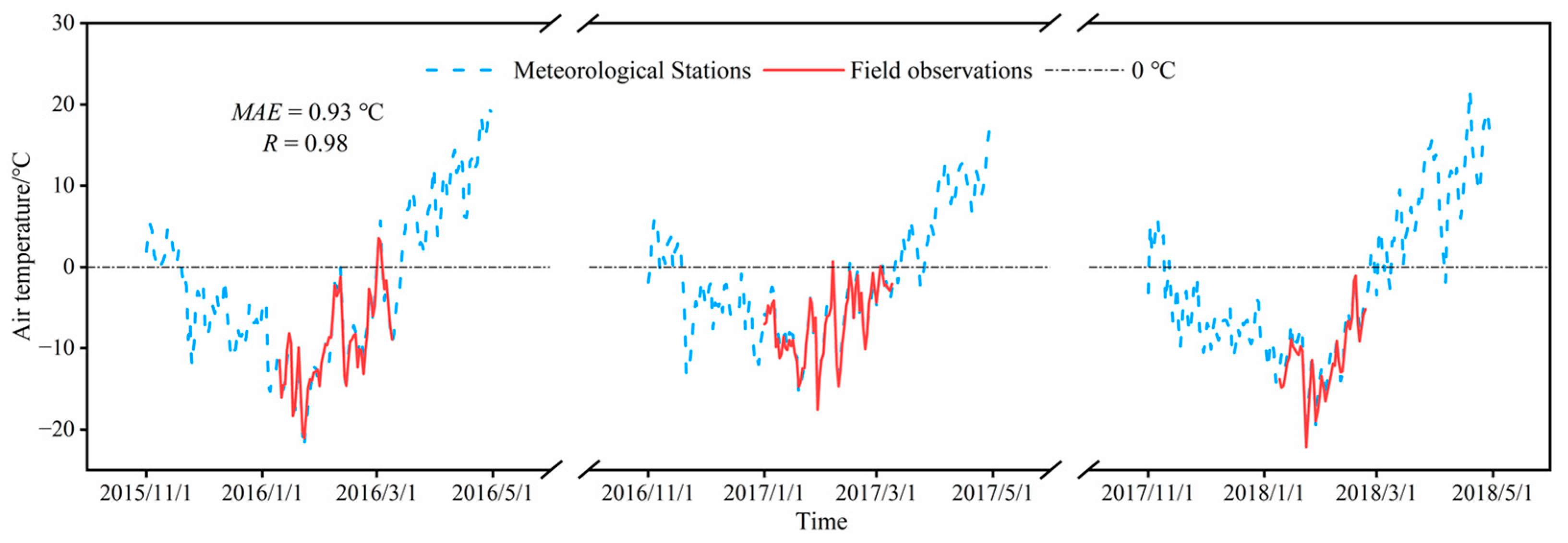
To accurately match the meteorological data of the ice-covered period, we selected the meteorological station data from the Dataset of Daily Climate Data from Chinese Surface Stations for Global Exchange. The data were released by the National Meteorological Information Center (NMIC) of the China Meteorological Administration (CMA) (http://data.cma.cn (accessed on 6 May 2022)). Four proximate meteorological stations measured these data at Baotou, Dongsheng, Linhe, and Urad Middle Banner (Figure 1). The daily mean, maximum, and minimum air temperatures of Wuliangsu Lake were obtained using the daily meteorological data according to the inverse distance weighted method. To verify the calculation, field observations from 2016 to 2018 were employed [27], using a PTWD sensor with a −40–80 °C measurement range and a ±0.04 °C precision. Furthermore, the comparison between them (Figure 2) shows that the mean absolute error (MAE) was 0.93°C, and the correlation coefficient (R) equaled = 0.98 for the daily mean air temperature. It indicates that the data can represent the natural meteorological conditions in Wuliangsu Lake.

3. Methods

3.1. Lake Ice Phenology Extraction

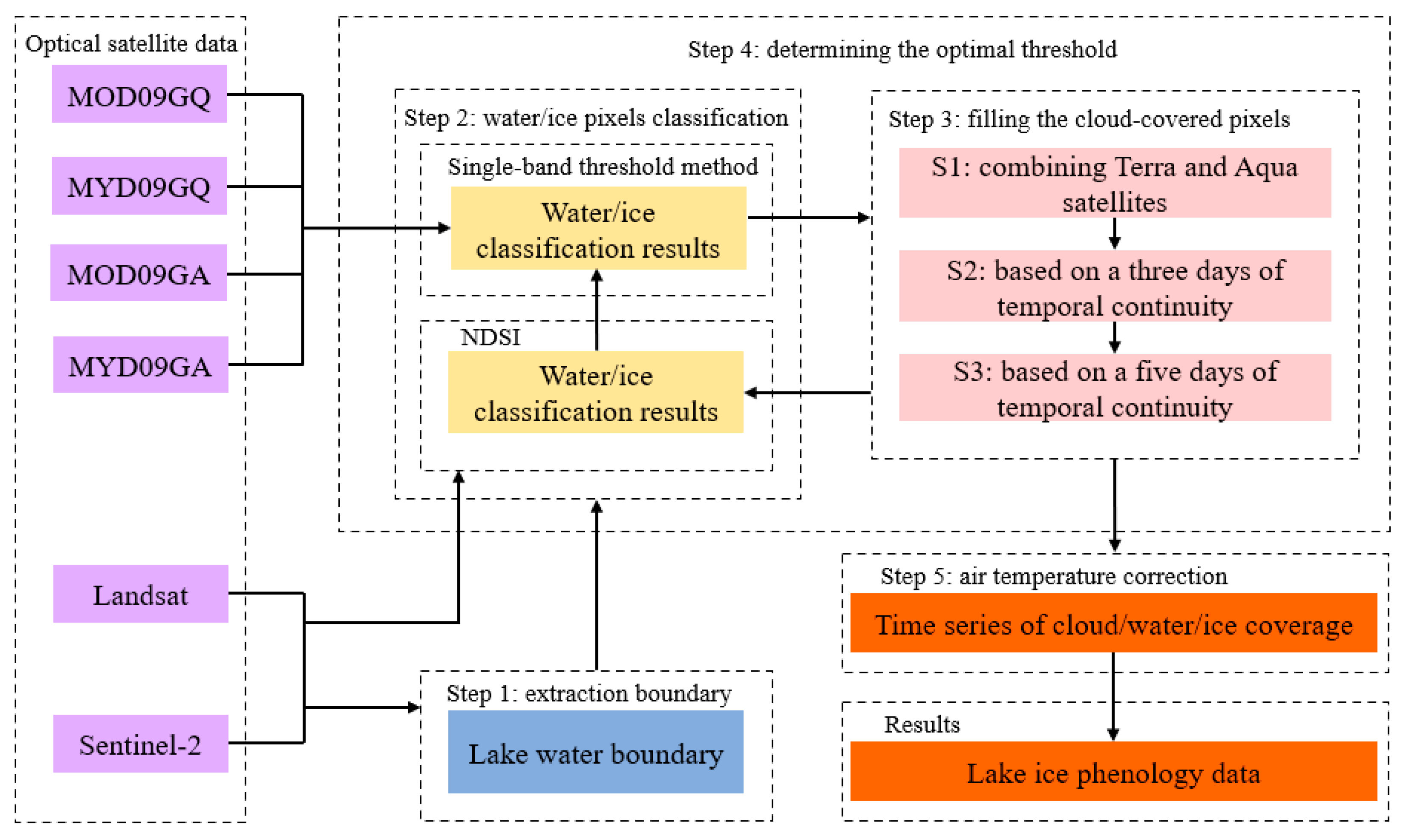
The algorithm for obtaining the lake wetland ice phenology can be divided into five steps (Figure 3). Step 1: The lake water boundary in Landsat and Sentinel-2 imageries are extracted. Step 2: The water/ice pixels within the lakes observed in MODIS, Landsat, and Sentinel-2 imageries are extracted. Step 3: The extracted results of MODIS products are processed to fill the cloud-covered pixels. Step 4: MODIS imagery classification results are compared with those of Landsat and Sentinel-2, with a higher spatial resolution to determine the optimal threshold for distinguishing water/ice pixels. Step 5: The ice phenology data are obtained from the time series of cloud/water/ice coverage after air temperature correction.

3.1.1. Extraction of Lake Water Boundary

Considering the interannual variation in aquatic plant extent, the lake water boundaries must be extracted for each year based on Landsat and Sentinel-2 imageries. We employed the Normalized Difference Water Index (NDWI) formula proposed by McFeeters [31]. It takes advantage of the fact that soil and vegetation usually have high near-infrared (NIR) reflectance, strongly absorbed by water. The green band improves the reflectance of water and can meet the need to distinguish reeds from water bodies.
Using Equation (1):
NDWI = Band   2 Band   4 Band   2 + Band   4
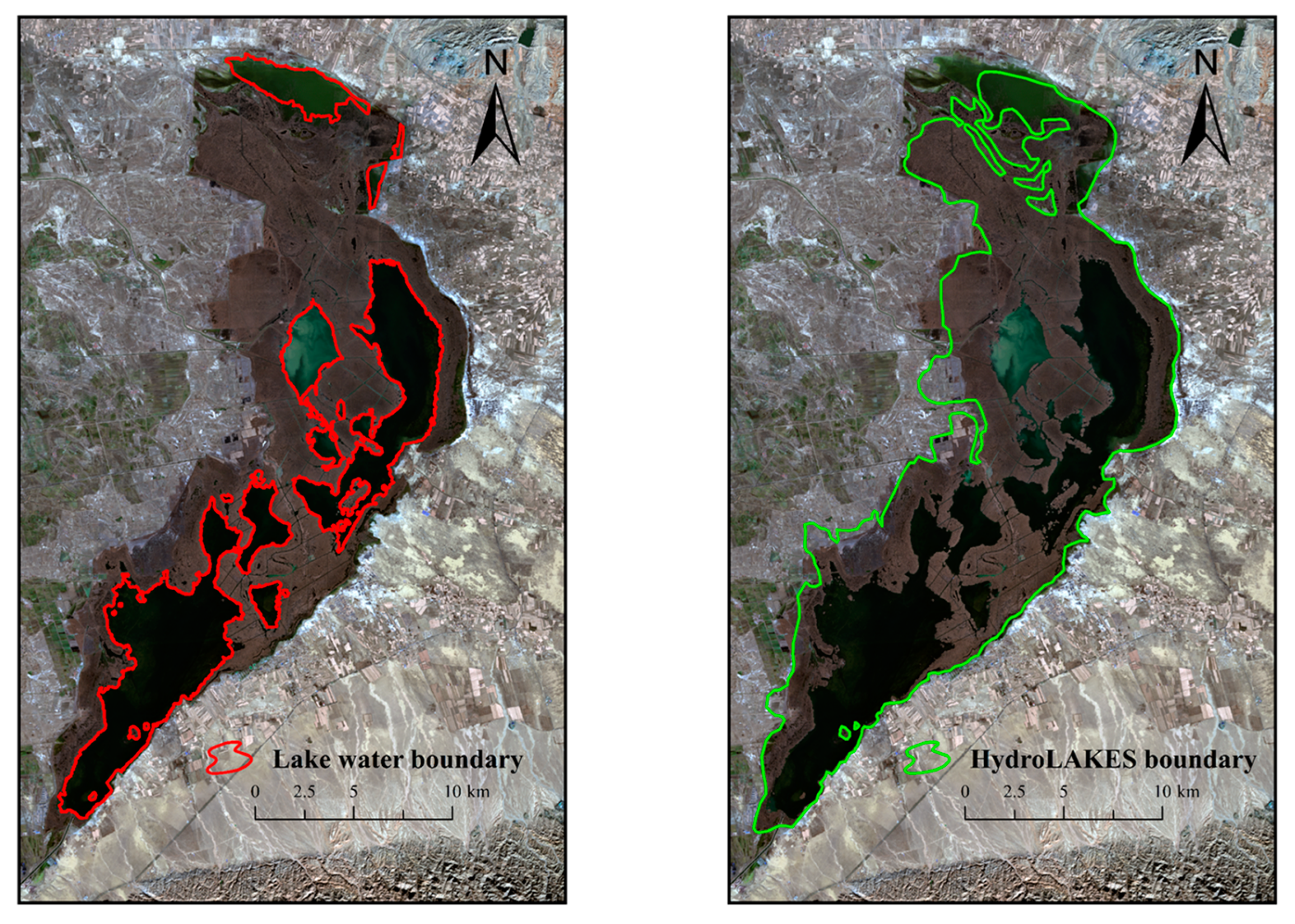
where Band 2 and Band 4 represent the reflectance of the green and NIR bands, respectively, in Landsat and Sentinel-2 products; the NDWI values range from −1 to 1; and a positive value represents a lake water extent that should be checked visually to minimize the influence of lakeshore pixels on water/ice discrimination. A comparison of the lake water boundary between the HydroLAKES dataset and the result of Equation (1) is shown in Figure 4. We observed that Equation (1) could effectively annul the influence of wetland aquatic plants on the lake water boundary and validly retain the valuable pixels in the lake water with higher accuracy. In contrast, the lake water boundary of the HydroLAKES dataset contains many aquatic plants. It is also less accurate at the intersection with land, leading to incorrect pixel statistics.

3.1.2. Extraction of Water and Ice Pixels

First of all, within the boundary of lake water, the single-band threshold was employed to extract water/ice pixels. Meanwhile, the reflectance band quality parameter QC_250M_1 in the MOD09GQ dataset can eliminate error pixels and categorize them into clouds, which can effectively use the information in the MOD09GQ dataset and ensure the accuracy of the threshold. The formula is as follows:
P i x e l s = {   ice ,                             Band   1 > a   water ,                   Band   1 < a
where Band 1 represents the reflectance of the red band in the MOD09GQ dataset and a represents the threshold to distinguish between water and ice.
Then, we employed the Normalized Difference Snow Index (NDSI) formula for Landsat and Sentinel-2 products [32]. The formula is as follows:
NDSI = Band   2 Band   5 Band   2 + Band   5
where Band 2 and Band 5 represent the reflectance of the green and shortwave infrared bands, respectively, in Landsat and Sentinel-2 products. NDSI of = 0.4 was selected as the threshold [20]. The vector boundary of water/ice was extracted with manual visual judgment, and the water/ice coverage in Landsat/Sentinel-2 imageries could be calculated.
Finally, the dynamic threshold method was employed to constantly modify the threshold a to change the water/ice classification results of the MOD09GQ dataset, and compared with the water/ice coverage area of Landsat and Sentinel-2 products with high spatial resolution to find the optimal threshold a.

3.1.3. Cloud Removal by Gap Filling

It is crucial to remove cloud pixels, which always affect optical imageries. The reflectivity band state parameter state_1 km_1 of MOD09GA and MYD09GA datasets, a 16-bit binary data with a spatial resolution of 1 km, was employed here. To retain the valuable pixels in the water bodies as much as possible, the cloud mixed and cloud shadow pixels were not considered in this paper. The specific method is similar to that of Zhang et al. [13]. The state_1km_1 value was first interpolated into a 250 m resolution image. Then, the cloud pixel was extracted by coding to synthesize a mask used to remove the cloud pixels in the daily corresponding Band 1 image. Zhang et al. [13] verified the method with 296 lakes, achieving excellent results. However, the method only removed the cloud pixels and did not fill the gaps under the removed clouds, thereby losing some relevant information such as extracting ice phenology. Therefore, a further filling process, i.e., cloud-covered pixel filling, was performed after cloud identification.
To improve the cloud gap filling accuracy, MOD09GQ from Terra satellite and MYD09GQ from the Aqua satellite were combined. For the same day, if the two satellite products were different in pixel classifications, the results of the Aqua satellite were reliable. The comparison with Landsat and Sentinel-2 products showed that the accuracy of Aqua was 71.4%, higher than 28.6% of Terra. The first step to fill the gaps (S1 in Figure 3) is shown in Equation (4), where P denotes pixels and output is the pixel type (water/ice) of the output satellite. It is divided into two cases: (1) if Aqua data are identified as water (ice) at A pixel, A pixel is defined as water (ice); (2) if Aqua data are identified as cloud at A pixel and Terra satellite is identified as water (ice) at A pixel, A pixel is defined as water (ice).
P ( A , output ) = { water / ice ,     if   P ( A , Aqua ) = water / ice                                                                                             water / ice ,     if   P ( A , Aqua ) = cloud   AND   P ( A , Terra ) = water / ice
Equation (4) can fill some but not all the cloud pixels’ gaps because the MOD09GQ and MYD09GQ datasets have missing values. Therefore, the second step uses the temporal continuity principle (S2 in Figure 3) to associate the type of A pixel on day t with the same pixel on days t − 1 and t + 1 [33]. The detail is if the A pixel on day t is a cloud pixel and is discriminated as water (ice) on days t − 1 and t + 1, then the pixel on day t is defined as water (ice). The formula is as follows:
P ( A , t ) = water / ice ,     if   P ( A , t 1 ) = P ( A , t + 1 ) = water / ice
Some cloud pixels that exist after applying Equation (5) are further calculated based on the five days of temporal continuity [33] (S3 in Figure 3). As shown in Equation (6), there are two cases: (1) if the A pixel is cloud on days t − 1 and t, and is water (ice) on days t − 2 and t + 1, then the A pixel is defined as water (ice) on days t − 1 and t; (2) if the A pixel is cloud on days t and t + 1, and is water (ice) on days t − 1 and t + 2, then the A pixel is defined as water (ice) on days t and t + 1.
{ P ( A , t ) = P ( A , t 1 ) = water / ice ,     if   P ( A , t 2 ) = P ( A , t + 1 ) = water / ice P ( A , t ) = P ( A , t + 1 ) = water / ice ,     if   P ( A , t + 2 ) = P ( A , t 1 ) = water / ice

3.1.4. Air Temperature Calibration

Once pixel types within the lake water boundary are defined, the number of water/ice pixels can be counted. The variations in the water/ice coverage can be obtained by analyzing the time series of satellite data. However, there are still some uncertain pixels despite the reduction of most of the cloud pixels. In addition, thin ice and mixed pixels on the lakeshore are unstable factors to distinguish between water/ice pixels. Therefore, air temperature removes outliers in the time series of water/ice coverage [13]. The basic principle is that the ice coverage on day t (I(t)) in the lake should not decrease when the mean air temperature on day t (T(t)) decreases, and I(t) should not increase when T(t) increases. However, the mean air temperature of a particular day cannot be chosen because it is not representative, rather it fluctuates frequently and greatly. Therefore, the mean air temperature within several days (2–50 days) before day t was calculated, and the highest correlation coefficient (−0.83) was found between the mean air temperature within 30 days before day t (T(t,30m)) and I(t). Hence, T(t,30m) was used as a dynamic air temperature correction to compare with the T(t) on day t, and then I(t) can be corrected according to the following equation:
{ I ( t ) = I ( t 1 ) ,     if   T ( t ) < T ( t , 30 m )   AND   I ( t ) < I ( t 1 ) I ( t ) = I ( t 1 ) ,     if   T ( t ) > T ( t , 30 m )   AND   I ( t ) > I ( t 1 )
After correcting I(t), the water coverage can be determined by W(t) = 1 − I(t)C(t), where C(t) is the cloud coverage on day t. To preserve the original pixel type as much as possible, Equation (7) was corrected only for the I(t) from November to March.

3.1.5. Extraction of Lake Ice Phenology

The I(t) during the ice-covered period is usually close to 1. The cloud pixels and mixed pixels also cause large fluctuations in I(t), which further affect the accuracy of the automatic extraction of ice phenology. Therefore, unlike a previous study [34] that used I(t) as the criterion, this paper used the W(t) to judge ice phenological dates. As shown in Equation (8), the freeze-up start (FUS) and freeze-up end (FUE) are defined as the date when W(t) first fell below 0.8 and 0.2 [35], respectively. Correspondingly, the break-up start (BUS) and break-up end (BUE) are defined as the date when W(t) was again above 0.2 and 0.8, respectively. Four periods can be calculated based on the four ice phenology dates. The freezing-up duration (FUD) is the duration process of reducing the W(t) in the lake (FUE–FUS). Corresponding to FUD, we chose BUE-BUS to calculate the break-up duration (BUD), while the ice cover duration (ICD) equaled BUE-FUS. The complete freezing duration (CFD) [36] is the period the lake surface is completely frozen; it equals BUS-FUE. In addition, to avoid errors in the automatic extraction results from less-than-ideal quality pixels during the ice-free period, Equation (8) discriminates these dates as T(t) drops to 0 °C each year.
{ FUS = Min ( t ) ,     if   W ( t ) < 0.8 FUE = Min ( t ) ,     if   W ( t ) < 0.2 BUS = Max ( t ) ,     if   W ( t ) > 0.2 BUE = Max ( t ) ,     if   W ( t ) > 0.8

3.2. Statistical Analysis

The linear regression was used to analyze the trends in the eight ice phenology characteristics of Wuliangsu Lake. Their trends were established for each characteristic. In addition, the mean absolute error (MAE), root mean square error (RMSE), and correlation coefficient (R) were calculated for comparisons of ice phenology dates for Wuliangsu Lake derived from filed observations and MODIS products.

4. Results

4.1. Determining the Optimal Threshold

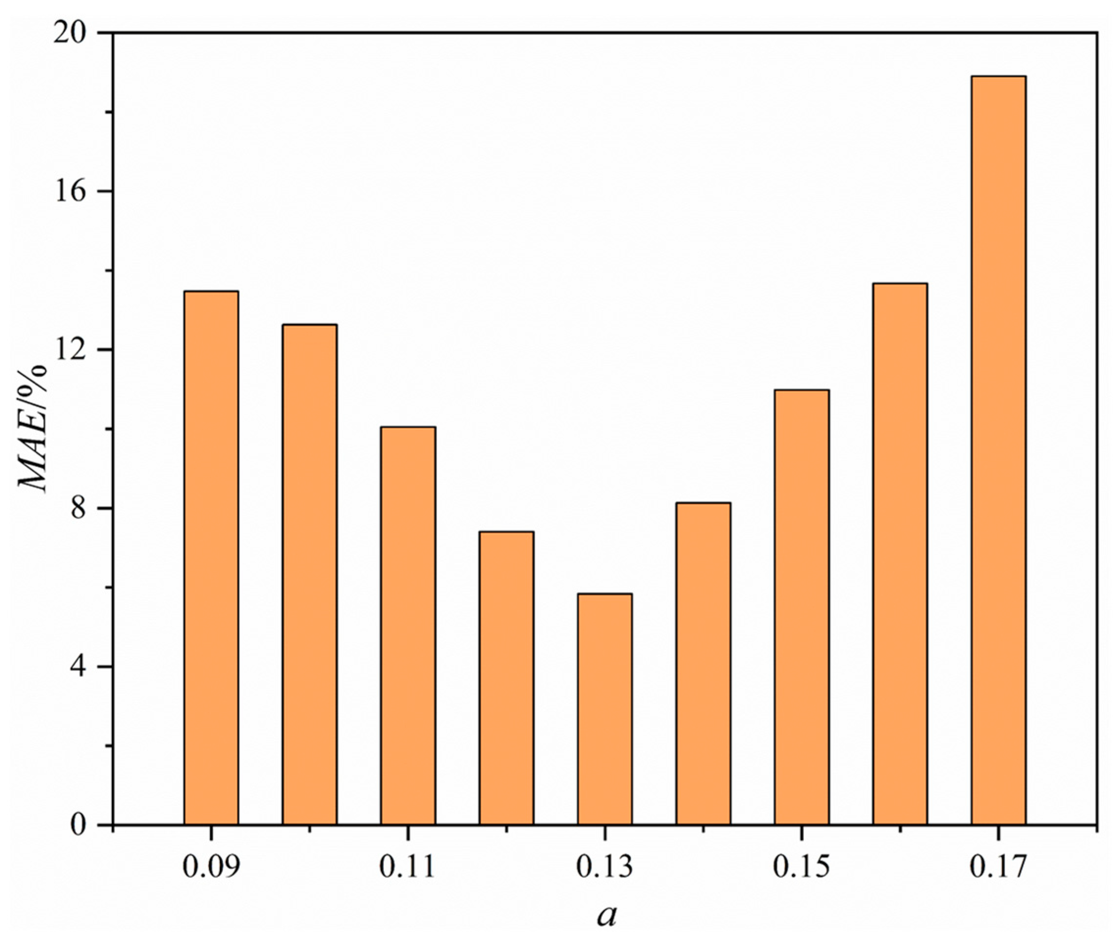
The threshold was set at 0.09–0.17 with a 0.01 interval (Section 3.1.2). The water/ice pixels in the MODIS products were extracted cyclically according to the dynamic threshold and single-band threshold methods. The classification results were transformed into water/ice coverage and compared with those of selected Landsat and Sentinel-2 imageries in the freezing/thawing period. The results show that the error was smallest when the threshold a was 0.13 (Figure 5), at which the MAE = 5.84% and R = 0.98.

4.2. Cloud Removal and Filling

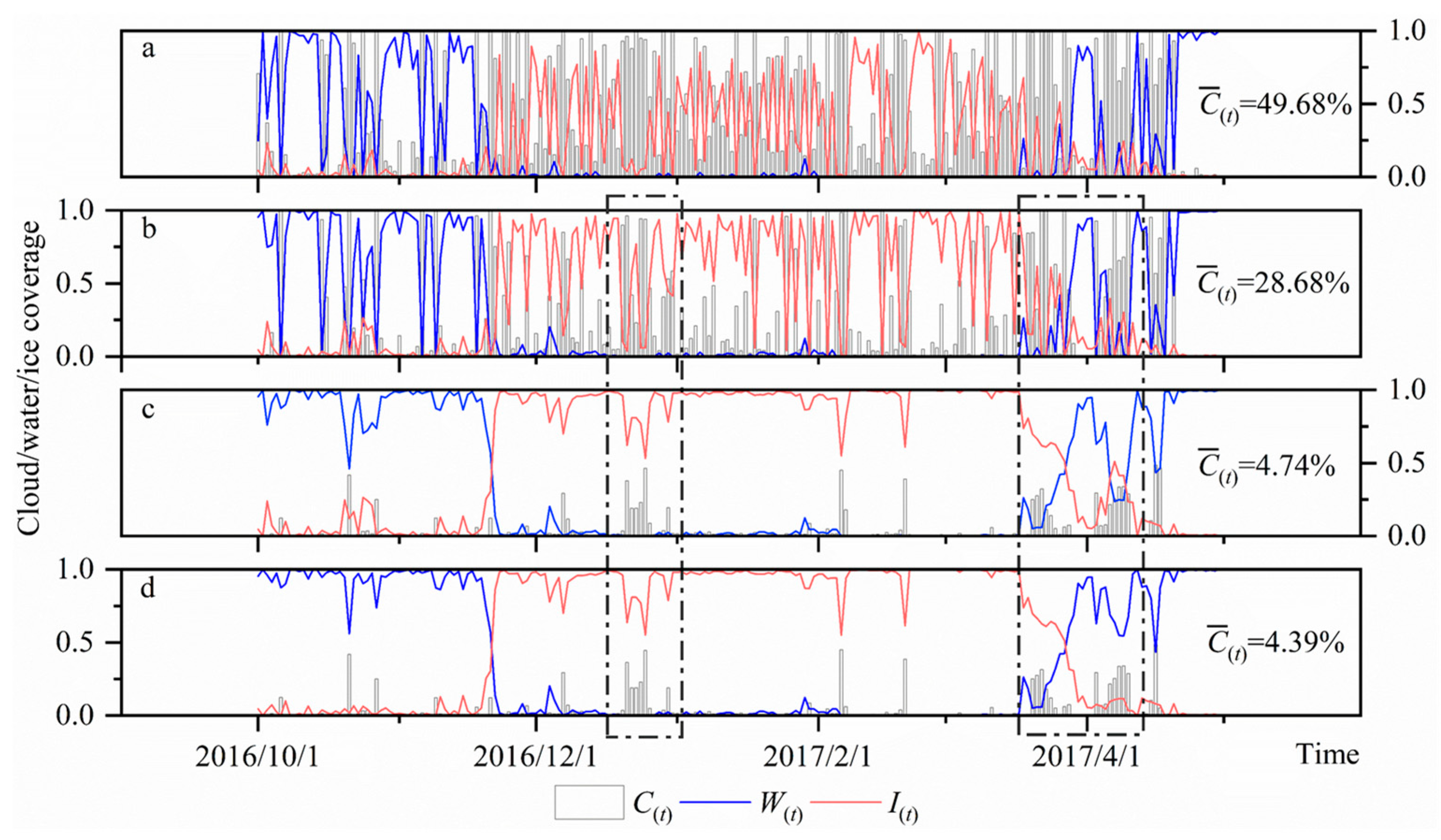
Figure 6 depicts the filling of the cloud-covered pixels using the threshold classification results according to Section 3.1.3. Before filling the cloud-covered pixels, the mean cloud coverage ( C ¯ ( t ) ) of Terra and Aqua satellite products was 43.41% in 2017. After combining the two satellite products (S1 in Figure 3), C ¯ ( t ) reduced to 28.68%. Using the temporal continuity method in three days (S2 in Figure 3), C ¯ ( t ) reduced again by 83.47%. Finally, C ¯ ( t ) reduced to 4.39%, according to the temporal continuity method in five days (S3 in Figure 3). This three-step cloud removal process reduced the C ¯ ( t ) by a total of 91.16%, which largely minimized the impact of clouds on water/ice classification results. It is noteworthy that the C(t) was still greater than 0.2 for several consecutive days after the complete cloud removal process (underlined box of Figure 6). The reason is that the calculation based on temporal continuity was needed in filling cloud-covered pixels for S2 and S3. Still, a higher C(t) for many consecutive days after S1 processing indirectly affected the cloud removal effect of S2 and S3. Therefore, if Aqua and Terra satellites are cloud-covered in the same area for many consecutive days, it would be difficult to remove the cloud and fill the area with natural surface categories.
Table 1 summarizes the cloud coverage of Wuliangsu Lake using MODIS data from October to next April between 2013 and 2022. We observed that 2016 had the highest cloud coverage during the study period after implementing S1 cloud removal. It is partly because the original C ¯ ( t ) before the cloud removal process was higher in the study period (41.30% and 52.01%). In addition, some data were missing for the Terra satellite in the 2016 h26v04 region which affected the calculation of the complete time series. Although the S1 cloud removal result indirectly affected those of S2, S2 was still the most effective step among the cloud removal processes, achieving 75.82% cloud removals. After the complete cloud removal process, the lowest C ¯ ( t ) was 2.95% in 2020, 8% lower in most years, thereby achieving a better filling cloud-covered pixels’ effect (Table 1). At the same time, this process filled in the actual pixels in the dataset with quality limitations, which vastly increased the accuracy of the extracted ice phenology data.

4.3. Air Temperature Correction

The cloud/water/ice coverage variations were obtained after filling the cloud-covered pixels. Although it is possible to clearly distinguish the ice phenology characteristics of Wuliangsu Lake in the last 10 years based on visual interpretation, unfilled cloud pixels and mixed pixels for the ice-covered period may lead to erroneous dates for the automatic extraction using Equation (8). Hence, an air temperature correction becomes necessary.
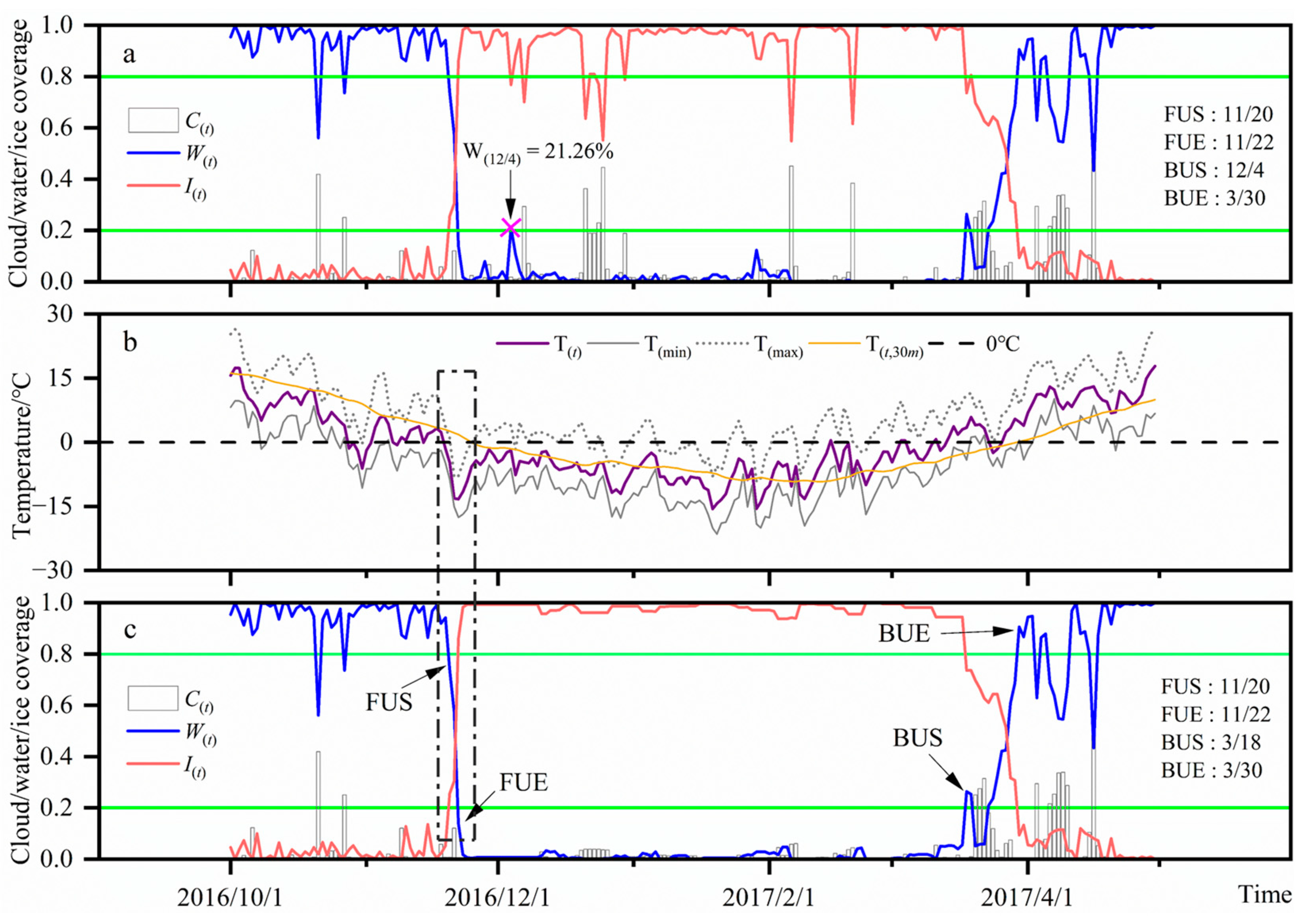
Taking 2017 as an example, Figure 7 compares cloud/water/ice coverage with and without temperature correction. Equation (8) automatically discriminated when T(t) < 0 °C for the first time on 28 October 2016. As T(t) stabilized below 0 °C, W(t) < 0.8 for the first time on 20 November 2016 and was, hence, extracted as the FUS date. When T(t) decreased rapidly and W(t) fell below 0.2 for the first time on 22 November 2016, the FUE date was extracted accordingly. Since W(12/4) = 21.26% on 4 December 2016, it was automatically extracted as the BUS date (Equation (7)). Then, 30 March 2017 was the BUE date when W(t) was later higher than 0.8.
Among them, W(t) was high on 2016/12/4 due to the cloud shadow in the part of Wuliangsu Lake in the MOD09GQ and MYD09GQ datasets (Figure 7a). It resulted in a lower reflectance than normal in that region, automatically classified as water pixels through the threshold. It further caused a wrong ice phenology date using Equation (8). After air temperature correction for I(t) from November to March (Figure 7c), the C ¯ ( t ) decreased from 4.39% to 2.96% in 2017. During the ice-covered period, the C(t) was approximately 0, and the sum of water-to-ice coverage was approximately 1. Thus, 18 March 2017 can be extracted accurately as the BUS dates. It proved the capability of air temperature correction, and selecting a stable T(t,30m) as the dynamic air temperature correction can effectively reduce the influence of cloud shadow and mixed pixels. This case would further improve the accuracy of Equation (8) for the automatic extraction of ice phenology dates.

4.4. Lake Wetland Ice Phenology

4.4.1. Ice Phenology

The ice phenology characteristics of Wuliangsu Lake during the study period are summarized in Table 2. On average, the Wuliangsu Lake started to freeze on 17 November, with the earliest FUS date being 9 November (2013, 2015) and the latest on 24 November (2014). The mean FUE date was 25 November, and the earliest FUE date was 16 November (2013), 15 days away from the latest FUE date. Wuliangsu Lake is shallow, generally having a short FUD (mean FUD = 7.1 days). The shortest FUD was two days, which occurred in 2017 (Figure 7). In addition, Wuliangsu Lake usually started melting on 25 March, with the earliest BUS appearing on 10 March (2013, 2021) and the latest on 25 March (2015). The CFD range and mean were 105–118 and 111.8 days, respectively. The average BUE date was 30 March, with the earliest and latest on 19 March (2021) and 30 March (2015, 2017), respectively. They resulted in a mean ICD of 126.5 days, while the longest ICD was 139 days in 2016.

4.4.2. Verification of Ice Phenology Data

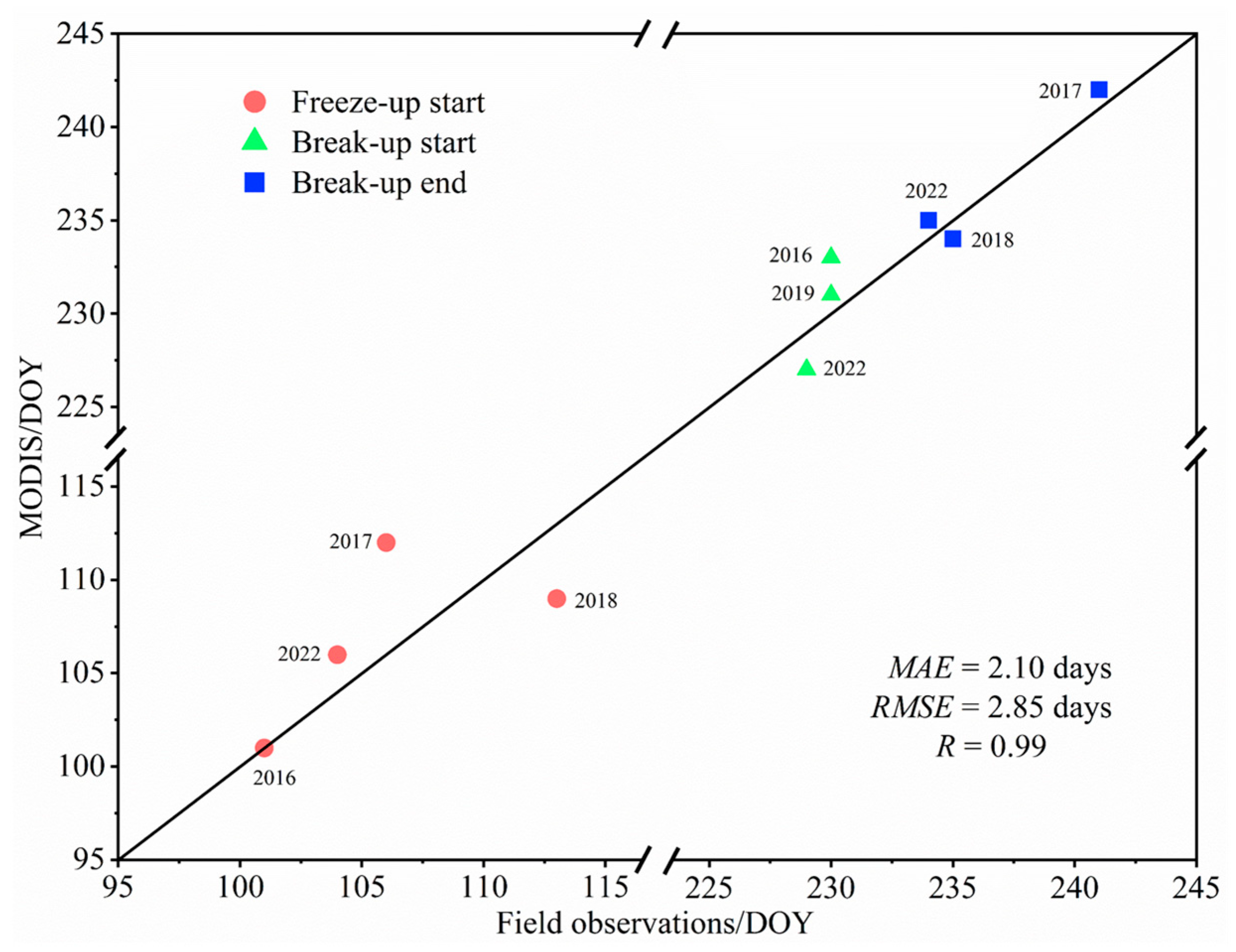
Field observations were conducted over four years (2016–2018, 2022) in Wuliangsu Lake, and the FUS, BUS, and BUE dates were recorded. Figure 8 depicts the comparisons between remote sensing results and field observation data. The R = 0.99, MAE = 2.10 days, and the root mean square error (RMSE) = 2.85 days. The agreement in Figure 8 argued for the feasibility of this study’s algorithm. Compared with the results of Zhang et al. [12], the current study recorded a small error in the ice phenology of Wuliangsu Lake. This achievement is the main benefit of enhancing the accuracy of extracting lake boundaries and filling cloud-covered pixels, thus obtaining more accurate lake surface cover types.

5. Discussion

5.1. Error Analysis

5.1.1. Satellite Products

Step 4 in Figure 3 can obtain classification thresholds that are more suitable for the conditions of the water bodies in Wuliangsu Lake, but the error still existed after the optimal threshold a = 0.13 was selected (Figure 5). The reason is related to the spatio-temporal resolution of the satellite products. For example, in Figure 9, the lake water and ice areas extracted from Landsat-8/Sentinel-2 products on 2 March 2021 were about 129.56 and 125.58 km2 based on the NDWI and NDSI formulas, respectively. It means the water area on 2 March 2021 was about 3.98 km2. However, the water area extracted from the MODIS product was about 6.06 km2 based on the threshold method, while the error in water coverage calculation was about 1.61%. This difference is mainly due to the complex shoreline shape of Wuliangsu Lake, and the inevitably adulterated mixed pixels with the 250 m spatial resolution in the MOD09GQ and MYD09GQ datasets (Figure 9c), despite the lake water boundary obtained using the NDWI formula. The same threshold classification and cloud removal process was conducted for the red band of the MOD09GA and MYD09GA datasets (Section 3.1.2 and Section 3.1.3). Due to its 500 m spatial resolution, fewer pure pixels at the reed/ice boundary and more mixed water/ice pixels at the water/ice boundary resulted in more pixel misclassifications than the MOD09GQ and MYD09GQ datasets (Figure 9d). In addition, the opening/closing period of Wuliangsu Lake ice cover is usually less than 10 days, while the temporal resolution of Landsat-7 and Landsat-8 imageries is 16 days. Therefore, the open/close date cannot be captured annually, leading to a lack of optical imageries with higher spatial resolution, unconducive to comparing MODIS products. Although this paper combines Sentinel-2 imageries with a revisit period of 5 days, it still needs to consider the influence of clouds on the three optical satellite products. Thus, the quantity and quality of satellite images can cause errors in the statistical results after threshold classification.

5.1.2. Observation Principle

The residual difference between field observations and MODIS data can be attributed to the observation principle. The angle of view limits field observations, relying more on the individual subjective discrimination of lake surface cover types. In contrast, satellite remote sensing can more comprehensively and objectively assess the whole lake. However, it is limited by clouds, thin ice, and mixed pixels. Meanwhile, filling the cloud-covered pixels by spatial and temporal characteristics of the MODIS products maximizes the error of two days on the extracted ice phenology dates. This phenomenon occurs because pixel filling requires two days of previous and subsequent classification results (Equation (6)). In addition, the thresholds of W(t) for judging the ice phenology dates were 0.2 and 0.8, instead of 0 and 1. Thus, this results in an advance or delay in the extracted dates, such as later FUS and BUS dates, and earlier FUE and BUE dates, which further affect the calculation of CFD and ICD. More importantly, during the lake surface’s freezing/thawing process, a “night freezing-day thawing” always occurs, affecting remote sensing and field results. For example, the absolute error of the FUS in 2017 was six days because the freezing–thawing cycle occurred at the beginning of the freezing period (Figure 7). The temporal resolution of MODIS products could not capture the variations on the lake surface within a day, and the field observers could not fully assess the overall surface condition of the lake, thus causing the maximum error during the comparison.

5.2. Trends of Ice Phenology

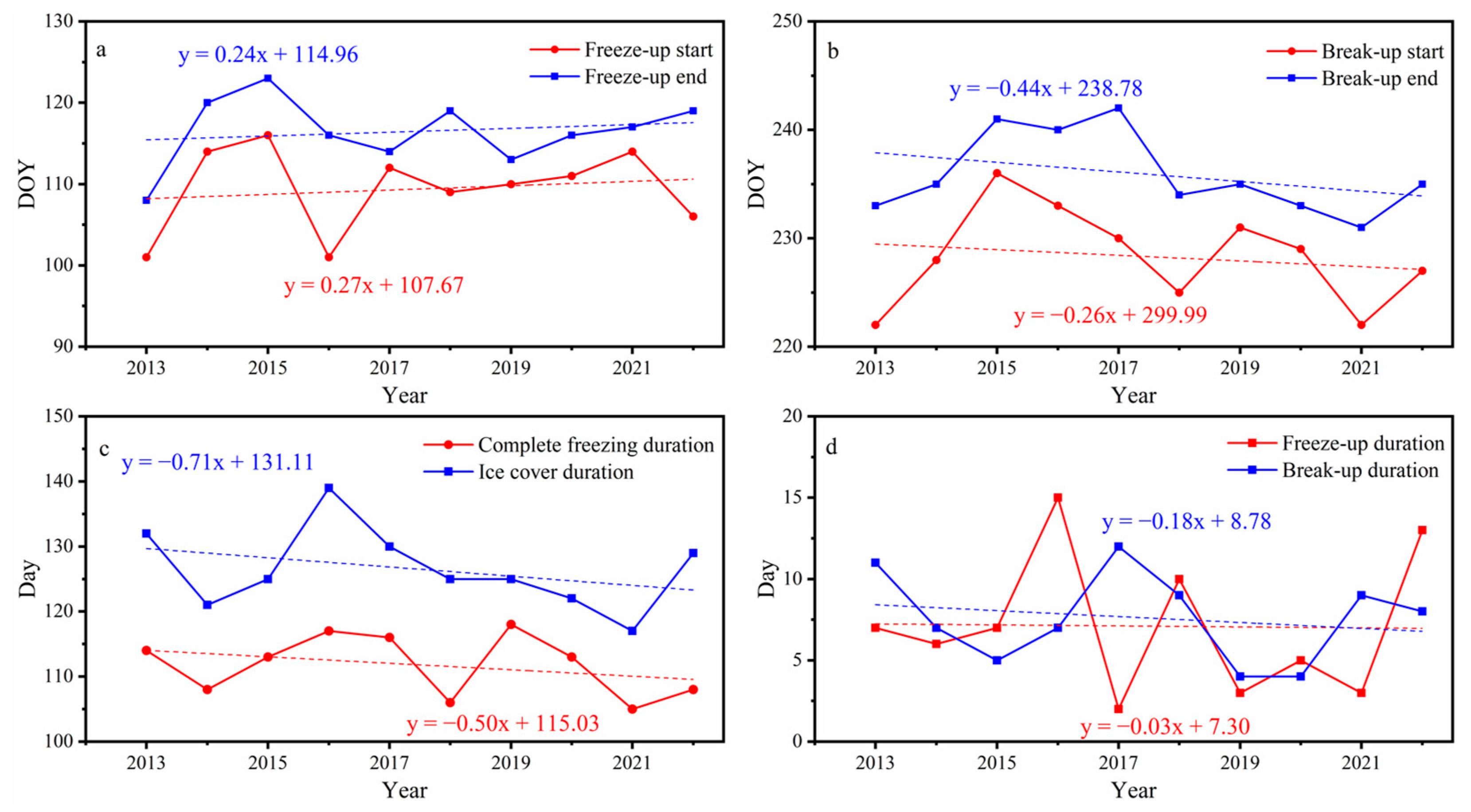
Figure 10 illustrates the linear trends of the ice phenology characteristics of Wuliangsu Lake. The FUS and the FUE dates show a delay trend (Figure 10a), with respective mean rates of 0.27 and 0.24 d/y. The BUS date is advanced by 0.26 d/y (Figure 10b), and the BUE date evinces a more obvious advancing trend with a 0.44 d/y rate. The CFD has a significant shortening trend (Figure 10c), with a mean rate of 0.50 d/y, which corresponds to the delay in the FUE date and the advance of the BUS date. The most dramatic variation in ice phenology is the ICD (Figure 10c), decreasing at −0.71 d/y. The FUD and BUD trends are unclear (Figure 10d), with −0.03 and −0.18 d/y mean rates, respectively. However, the FUD fluctuation is high, which is associated with climate change and the peculiarity of Wuliangsu Lake. For example, the FUS date was determined on 20 November when the T(t) was negative for two consecutive days in 2017, and the FUD was only two days (Figure 7c). The reason for this situation is that, on the one hand, the shallow water body of Wuliangsu Lake has a small heat capacity. Therefore, the rapid air temperature fluctuation will significantly impact the water body (Figure 7b). On the other hand, although the daily mean air temperature has just reduced to 0 °C, the minimum air temperature has dropped to a level relatively lower than the freezing point because of the large temperature difference between day and night (mean = 12.4 °C). It benefits the “night freezing-day thawing” cycle on the lake surface, and a stable ice cover forms only when the water column is well-mixed.

6. Conclusions

Ice phenology in the shallow Wuliangsu Lake, with a significant portion of wetland in the northwest China arid area, was investigated using optical satellite data with high spatial and temporal resolution. A new method was developed and proved to effectively remove the influence of aquatic plants and clouds from the investigation domain.
Landsat-7, Landtsat-8, and Sentinel-2 imageries were first employed to extract the lake water boundary according to the NDWI formula and visual judgement. Moreover, based on the dynamic threshold and single-band threshold methods, an optimal threshold of a = 0.13 was determined for distinguishing water/ice pixels within the lake water boundary using the MODIS reflectivity products. Then, the time series of water/ice coverage was obtained. The series compared well with the results of Landsat-7, Landsat-8, and Sentinel-2 imageries during the opening/closing period of ice cover, with the MAE of 5.87%. In addition, the cloud-covered pixels in optical satellite imageries were removed using the state_1km_1 parameter of MODIS products, which filled 85.14% of the cloud-covered pixels and reduced the mean cloud coverage to less than 8% in most years. Finally, the influence of the remaining cloud and mixed pixels was further reduced by the air temperature correction, thus improving the accuracy of the ice phenology date.
According to these processes, we extracted the ice phenology characteristics of Wuliangsu Lake between 2013 and 2022, which correlated well with the field observations, with R = 0.99 and MAE = 2.10 days for the FUS, BUS, and BUE dates. We observed that Wuliangsu Lake usually starts to freeze from mid to late November every year, lasting until late March. The overall trend of FUS and FUE dates in the Wuliangsu Lake was delayed, with a mean rate of −0.27 and −0.24 d/y, respectively, and the BUS and BUE dates were advanced, with 0.26 and 0.44 d/y mean rates, respectively. Among the ice phenology characteristics, the most significant trend was the ICD, meaning 126.5 days and decreases by a mean rate of −0.71 d/y. Overall, the FUD and BUD trends are not clear; they exhibit a mean duration of 7.1 and 7.6 days, respectively, which are smaller than those found in most lakes on the Qinghai-Tibet Plateau [8]. This difference could be attributed to the peculiar shallowness of Wuliangsu Lake, which has a small heat capacity of the water body itself and requires less heat for freezing and melting, so the duration is shorter.
The present method has some advantages over previous studies. First, it can effectively remove the influence of aquatic plants in the lake wetland on the water/ice pixels’ discrimination and accurately identify the lake water boundary rather than the outer lake boundary. Secondly, it can reduce the influence of clouds on optical satellite imageries, satisfying the need for the automatic extraction of lake wetland ice phenology. However, the effect of mixed pixels, thin ice, and partially unremoved cloud pixels on pixel type discrimination could not be completely avoided. Although, the reflectance MODIS product with the highest spatial resolution reflectance dataset of the MODIS product was chosen to distinguish between water and ice. This issue is expected to be further analyzed as technology improves and field observations increase. Nevertheless, based on the technical basis of this study, it is possible to perform calculations on longer time scales in the future with acceptable accuracy, and then explore the relationship between wetland lake ice phenology and climate change.

Author Contributions

Formal calculation, analysis, writing—original draft, P.H.; analysis, supervision, conceptualization, P.L.; writing—review and conceptualization, B.C.; writing—review and editing, L.Z., Q.W. and Z.L. All authors have read and agreed to the published version of the manuscript.

Funding

This research was supported by the National Key Research and Development Program of China (Grant No. 2019YFE0197600), the LiaoNing Revitalization Talents Program (Grant No. XLYC2007033), the National Natural Science Foundation of China (Grant Nos. 41922045, 41876213 and 52211530038), and the Academy of Finland (350576).

Data Availability Statement

MODIS products can be downloaded from https://ladsweb.modaps.eosdis.nasa.gov/ (accessed on 6 May 2022); Landsat and Sentinel-2 products can be downloaded from https://earthexplorer.usgs.gov/ (accessed on 6 May 2022); The meteorological data from the NMIC of the CMA can be downloaded from http://data.cma.cn (accessed on 6 May 2022).

Acknowledgments

We thank the editor and anonymous reviewers for their comments, which considerably improved this work.

Conflicts of Interest

The authors declare no conflict of interest.

References

  1. Campbell, I.C.; Poole, C.; Giesen, W.; ValboJorgensen, J. Species diversity and ecology of Tonle Sap Great Lake, Cambodia. Aquat. Sci. 2006, 68, 355–373. [Google Scholar] [CrossRef]
  2. Kim, J.G. Response of sediment chemistry and accumulation rates to recent environmental changes in the Clear Lake watershed, California, USA. Wetlands 2003, 23, 95–103. [Google Scholar] [CrossRef]
  3. Leppäranta, M.; Wen, L.J. Ice Phenology in Eurasian Lakes over Spatial Location and Altitude. Water 2022, 14, 1037. [Google Scholar] [CrossRef]
  4. Bernhardt, J.; Engelhardt, C.; Kirillin, G.; Matschullat, J. Lake ice phenology in Berlin-Brandenburg from 1947–2007: Observations and model hindcasts. Clim. Change 2012, 112, 791–817. [Google Scholar] [CrossRef]
  5. Rigosi, A.; Carey, C.C.; Ibelings, B.W.; Brookes, J.D. The interaction between climate warming and eutrophication to promote cyanobacteria is dependent on trophic state and varies among taxa. Limnol. Oceanogr. 2014, 59, 99–114. [Google Scholar] [CrossRef] [Green Version]
  6. Zdorovennova, G.; Palshin, N.; Golosov, S.; Efremova, T.; Belashev, B.; Bogdanov, S.; Terzhevik, A. Dissolved Oxygen in a Shallow Ice-Covered Lake in Winter: Effect of Changes in Light, Thermal and Ice Regimes. Water 2021, 13, 2435. [Google Scholar] [CrossRef]
  7. Scheffers, B.R.; Meester, L.D.; Bridge, T.C.L.; Hoffmann, A.A.; Pandolfi, J.M.; Corlett, R.T.; Butchart, S.H.M.; Pearce-Kelly, P.; Kovacs, K.M.; Dudgeon, D.; et al. The broad footprint of climate change from genes to biomes to people. Science 2016, 354, aaf7671. [Google Scholar] [CrossRef] [PubMed]
  8. Kropáček, J.; Maussion, F.; Chen, F.; Hoerz, S.; Hochschild, V. Analysis of ice phenology of lakes on the Tibetan Plateau from MODIS data. Cryosphere 2013, 7, 287–301. [Google Scholar] [CrossRef] [Green Version]
  9. Qiu, Y.; Xie, P.; Leppäranta, M.; Wang, X.; Lemmetyinen, J.; Lin, H.; Shi, L. MODIS-based Daily Lake Ice Extent and Coverage dataset for Tibetan Plateau. Big Earth Data 2019, 3, 170–185. [Google Scholar] [CrossRef] [Green Version]
  10. Walsh, S.E.; Vavrus, S.J.; Foley, J.A.; Fisher, V.A.; Wynne, R.H.; Lenters, J.D. Global patterns of lake ice phenology and climate: Model simulations and observations. J. Geophys. Res.-Atmos. 1998, 3, 28825–28837. [Google Scholar] [CrossRef]
  11. Brown, L.C.; Duguay, C.R. The response and role of ice cover in lake-climate interactions. Prog. Phys. Geogr. 2010, 34, 671–704. [Google Scholar] [CrossRef]
  12. Han, W.; Huang, C.; Duan, H.; Gu, J.; Hou, J. Lake Phenology of Freeze-Thaw Cycles Using Random Forest: A Case Study of Qinghai Lake. Remote Sens. 2020, 12, 4098. [Google Scholar] [CrossRef]
  13. Zhang, S.; Pavelsky, T.M. Remote Sensing of Lake Ice Phenology across a Range of Lakes Sizes, ME, USA. Remote Sens. 2019, 11, 1718. [Google Scholar] [CrossRef] [Green Version]
  14. Geldsetzer, T.; Sanden, J.V.D.; Brisco, B. Monitoring lake ice during spring melt using RADARSAT-2 SAR. Can. J. Remote Sens. 2010, 36, S391–S400. [Google Scholar] [CrossRef]
  15. Meier, W.N.; Dai, M. High-resolution sea-ice motions from AMSR-E imagery. Ann. Glaciol. 2006, 44, 352–356. [Google Scholar] [CrossRef] [Green Version]
  16. Mack, S.; Padman, L.; Klinck, J. Extracting tidal variability of sea ice concentration from AMSR-E passive microwave single-swath data: A case study of the Ross Sea. Geophys. Res. Lett. 2013, 40, 547–552. [Google Scholar] [CrossRef] [Green Version]
  17. Tanaka, Y.; Tateyama, K.; Kameda, T.; Hutchings, J.K. Estimation of melt pond fraction over high-concentration Arctic sea ice using AMSR-E passive microwave data. J. Geophys. Res. Oceans 2016, 121, 7056–7072. [Google Scholar] [CrossRef]
  18. Tuttle, S.E.; Roof, S.R.; Retelle, M.J.; Werner, A.; Gunn, G.E.; Bunting, E.L. Evaluation of Satellite-Derived Estimates of Lake Ice Cover Timing on Linnévatnet, Kapp Linné, Svalbard Using In-Situ Data. Remote Sens. 2022, 14, 1311. [Google Scholar] [CrossRef]
  19. Šmejkalová, T.; Edwards, M.; Dash, J. Arctic lakes show strong decadal trend in earlier spring ice-out. Sci Rep. UK 2016, 6, 38449. [Google Scholar] [CrossRef]
  20. Cai, Y.; Ke, C.Q.; Li, X.; Zhang, G.; Duan, Z.; Lee, H. Variations of Lake Ice Phenology on the Tibetan Plateau From 2001 to 2017 Based on MODIS Data. J. Geophys. Res. Atmos. 2019, 124, 825–843. [Google Scholar] [CrossRef]
  21. Williamson, A.G.; Banwell, A.F.; Willis, I.C.; Arnold, N.S. Dual-satellite (Sentinel-2 and Landsat 8) remote sensing of supraglacial lakes in Greenland. Cryosphere 2018, 12, 3045–3065. [Google Scholar] [CrossRef] [Green Version]
  22. Zhang, X.; Wang, K.; Kirillin, G. An Automatic Method to Detect Lake Ice Phenology Using MODIS Daily Temperature Imagery. Remote Sens. 2021, 13, 2711. [Google Scholar] [CrossRef]
  23. Wu, Y.H.; Duguay, C.R.; Xu, L.L. Assessment of machine learning classifiers for global lake ice cover mapping from MODIS TOA reflectance data. Remote Sens. Environ. 2021, 253, 112206. [Google Scholar] [CrossRef]
  24. Messager, M.L.; Lehner, B.; Grill, G.; Nedeva, I.; Schmitt, O. Estimating the volume and age of water stored in global lakes using a geo-statistical approach. Nat. Commun. 2016, 7, 13603. [Google Scholar] [CrossRef]
  25. Sharma, S.; Blagrave, K.; Filazzola, A.; Imrit, M.A.; Hendricks Franssen, H.J. Forecasting the Permanent Loss of Lake Ice in the Northern Hemisphere Within the 21st Century. Geophys. Res. Lett. 2021, 48, e2020GL091108. [Google Scholar] [CrossRef]
  26. Tai, X.N.; Wang, N.L.; Wu, Y.W.; Zhang, Y.J. Lake ice phenology variations and influencing factors of Selin Co from 2000 to 2020. J. Lake Sci. 2022, 34, 334–348. [Google Scholar] [CrossRef]
  27. Lu, P.; Cao, X.W.; Li, G.Y.; Huang, W.F.; Leppäranta, M.; Arvola, L.; Li, Z.J. Mass and Heat Balance of a Lake Ice Cover in the Central Asian Arid Climate Zone. Water 2020, 12, 2888. [Google Scholar] [CrossRef]
  28. Huang, W.F.; Zhao, W.; Zhang, C.; Leppranta, M.; Li, Z.J.; Li, R.; Lin, Z.J. Radiative penetration dominates the thermal regime and energetics of a shallow ice-covered lake in an arid climate. Cryosphere 2021, 16, 1793–1806. [Google Scholar] [CrossRef]
  29. Duan, X.; Wang, X.; Mu, Y.; Ouyang, Z. Seasonal and diurnal variations in methane emissions from Wuliangsu Lake in arid regions of China. Atmos. Environ. 2005, 39, 4479–4487. [Google Scholar] [CrossRef]
  30. Cheng, B.; Xie, F.; Lu, P.; Huo, P.Z.; Leppäranta, M. The role of lake heat flux in the growth and melting of ice. Adv. Polar Sci. 2021, 32, 364–373. [Google Scholar] [CrossRef]
  31. McFeeters, S.K. The use of the Normalized Difference Water Index (NDWI) in the delineation of open water features. Int. J. Remote Sens. 1996, 17, 1425–1432. [Google Scholar] [CrossRef]
  32. Hall, D.K.; Riggs, G.A.; Salomonson, V.V. Algorithm Theoretical Basis Document (ATBD) for the MODIS Snow and Sea Ice-Mapping Algorithms; NASA: Greenbelt, MD, USA, 2001. Available online: https://modis-snow-ice.gsfc.nasa.gov/?c=atbd&t=atbd (accessed on 15 January 2022).
  33. Gafurov, A.; Bárdossy, A. Cloud removal methodology from MODIS snow cover product. Hydrol. Earth Syst. Sci. 2009, 13, 1361–1373. [Google Scholar] [CrossRef] [Green Version]
  34. Yang, Q.; Song, K.; Wen, Z.; Hao, X.; Fang, C. Recent trends of ice phenology for eight large lakes using MODIS products in Northeast China. Int. J. Remote Sens. 2019, 40, 5388–5410. [Google Scholar] [CrossRef]
  35. Yang, Q.; Song, K.; Ha, X.; Wen, Z.; Tan, Y.; Li, W. Investigation of spatial and temporal variability of river ice phenology and thickness across Songhua River Basin, northeast China. Cryosphere 2020, 14, 3581–3593. [Google Scholar] [CrossRef]
  36. Duguay, C.R.; Bernier, M.; Gauthier, Y.; Kouraev, A. Remote Sensing of Lake and River Ice; Wiley: Hoboken, NJ, USA, 2014; ISBN 9781118368909. [Google Scholar]
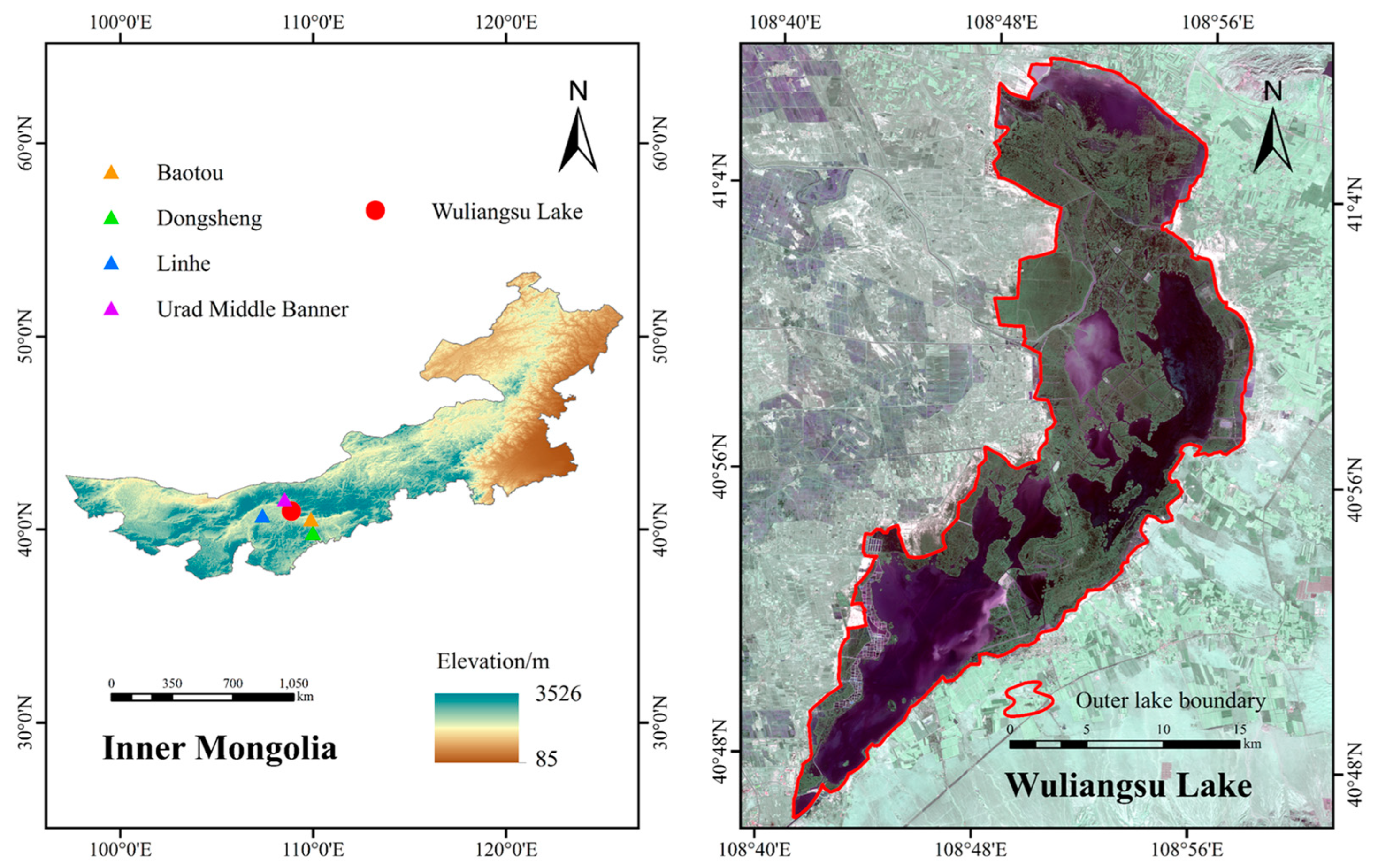
Figure 1. Location of the Wuliangsu Lake (the image on the right is the Sentinel-2’s imagery on 2 November 2020, the outer lake boundary contains lake water and extensive aquatic plants).
Water 14 03307 g001
Figure 2. Comparison of daily mean air temperature between meteorological stations and field observations from 2016 to 2018. (MAE is the mean absolute error, R is the correlation coefficient).
Water 14 03307 g002
Figure 3. Algorithm flow chart.
Water 14 03307 g003
Figure 4. Comparison of the lake water boundary between the HydroLAKES dataset and the result of the NDWI formula in Wuliangsu Lake (the Landsat-8 image on 7 November 2013 was the selected example).
Water 14 03307 g004
Figure 5. Mean absolute error (MAE) of the comparison between the water area extracted by MODIS product through the dynamic threshold a and that extracted by Landsat/Sentinel-2 product.
Water 14 03307 g005
Figure 6. Cloud removal results for Wuliangsu Lake in 2017. (a) Original Aqua MODIS; (b) after S1 calculation; (c) after S2 calculation; (d) after S3 calculation (C(t), W(t), and I(t) denote cloud, water, and ice coverage, respectively; C ¯ ( t ) denotes the mean cloud coverage. The underlined box marks high C(t)).
Water 14 03307 g006
Figure 7. Daily cloud/water/ice coverage and air temperatures in Wuliangsu Lake in 2017. (a) Without temperature correction. (b) Daily mean air temperature (T(t)), daily minimum air temperature (T(min)), daily maximum air temperature (T(max)), and mean air temperature of the previous 30 days (T(t,30m)) after calculating at the meteorological stations near Wuliangsu Lake. (c) With air temperature correction. (The two green lines indicate the two thresholds for extracting ice phenology dates, and the four arrows from left to right indicate freeze-up start (FUS), freeze-up end (FUE), break-up start (BUS), and break-up end (BUE), respectively).
Water 14 03307 g007
Figure 8. Comparisons of ice phenology dates for Wuliangsu Lake derived from filed observation and MODIS products (DOY means the day of the year relative to 1 August, R is the correlation coefficient, MAE is the mean absolute error, and RMSE is the root mean square error).
Water 14 03307 g008
Figure 9. Comparisons of the water area extracted by Landsat-8, Sentinel-2, and MODIS products (selected for 2 March 2021).
Water 14 03307 g009
Figure 10. The ice phenology characteristics and their trends for Wuliangsu Lake from 2013 to 2022. (a) Freeze-up dates and their trends. (b) Break-up dates and their trends. (c) Complete freezing duration and ice cover duration and their trends. (d) Freeze-up and break-up durations and their trends. (Date is based on the annual cumulative day method, for example, 14 November 2021 is the 106th day of 2022).
Water 14 03307 g010
Table 1. Comparison of cloud cover with and without cloud removal for Wuliangsu Lake from 2013 to 2022.
MeanMaximumMinimum
Original Terra38.67%42.30% (2015)31.54% (2014)
Original Aqua47.71%52.20% (2013)38.72% (2020)
S128.83%33.06% (2016)22.99% (2014)
S26.97%9.52% (2018)3.19% (2020)
S36.42%8.93% (2018)2.95% (2020)
Table 2. Ice phenology of Wuliangsu Lake between 2013 and 2022. (Date is expressed in mm/dd).
FUSFUEBUSBUEFUDBUDCFDICD
201311/911/163/103/21711114132
201411/2211/283/173/2467108121
201511/2412/13/253/3075113125
201611/911/243/223/29157117139
201711/2011/223/183/30212116130
201811/1711/273/143/23109106125
201911/1811/213/203/2434118125
202011/1911/243/183/2254113122
202111/2211/253/103/1939105117
202211/1411/273/163/24138108129
Average11/1711/253/173/257.17.6111.8126.5
Max11/2412/13/253/301512118139
Min11/911/163/103/1924105117
Publisher’s Note: MDPI stays neutral with regard to jurisdictional claims in published maps and institutional affiliations.