Article

Real-Time Leak Diagnosis in Water Distribution Systems Based on a Bank of Observers and a Genetic Algorithm

by
Adrián Navarro-Díaz
1,
Jorge Alejandro Delgado-Aguiñaga
2,*,
Ildeberto Santos-Ruiz
3 and
Vicenç Puig
4
1
Tecnológico de Monterrey, Escuela de Ingeniería y Ciencias, Av. General Ramón Corona 2514, Zapopan C.P. 45138, Mexico
2
Centro de Investigación, Innovación y Desarrollo Tecnológico CIIDETEC-UVM, Universidad del Valle de México, Periférico Sur Manuel Gómez Morín 8077, Tlaquepaque C.P. 45601, Mexico
3
Tecnológico Nacional de México/Instituto Tecnológico de Tuxtla Gutiérrez, TURIX-Dynamics Diagnosis and Control Group, Carretera Panamericana S/N, Tuxtla Gutiérrez C.P. 29050, Mexico
4
Institut de Robòtica i Informàtica Industrial, CSIC-UPC, C/Llorens i Artigas 4-6, 08028 Barcelona, Spain
*
Author to whom correspondence should be addressed.
Water 2022, 14(20), 3289; https://doi.org/10.3390/w14203289
Submission received: 1 September 2022 / Revised: 1 October 2022 / Accepted: 9 October 2022 / Published: 18 October 2022
(This article belongs to the Section Water Resources Management, Policy and Governance)

Abstract

:
The main contribution of this paper is to present a novel solution for the leak diagnosis problem in branched pipeline systems considering the availability of pressure head and flow rate sensors on the upstream (unobstructed) side and the downstream (constricted) side. This approach is based on a bank of Kalman filters as state observers designed on the basis of the classical water hammer equations and a related genetic algorithm (GA) which includes a fitness function based on an integral error that helps obtaining a good estimation despite the presence of noise. For solving the leak diagnosis problem, three stages are considered: (a) the leak detection is performed through a mass balance; (b) the region where the leak is occurring is identified by implementing a reduced bank of Kalman filters which localize the leak by sweeping all regions of the branching pipeline through a GA that reduces the computational effort; (c) the leak position is computed through an algebraic equation derived from the water hammer equations in steady-state. To assess this methodology, experimental results are presented by using a test bed built at the Tuxtla Gutiérrez Institute of Technology, Tecnológico Nacional de México (TecNM). The obtained results are then compared with those obtained using a classic extended Kalman filter which is widely used in solving leak diagnosis problems and it is highlighted that the GA approach outperforms the EKF in two cases whereas the EKF is better in one case.

1. Introduction

Nowadays, a safe fluid transportation process is a challenging issue since natural and/or abnormal events as aging pipes but also illegal intrusion could cause leaks, which in turn, produce economic losses, disasters and environmental pollution. In the last decades, legislators have reinforced laws to protect the environment against pollution by demanding to guarantee a safe fluid transportation process. The scientific community has paid attention to this problem and several pipeline monitoring techniques have been developed from different perspectives to reduce the impact of undesirable events, such as leaks, no matter what fluid is transported. In particular, taking care of water is of the special interest since it ensures the safety of water and is directly related to public health issues due to its worldwide inherent importance. Such techniques can be divided in two main approaches: external methods and model-based methods. The first ones use external equipment such as acoustic systems, electronic listening sticks, infra-red thermography, etc., to determine the leak location (theses methods are often expensive, require experienced user and most of the time it is require to use them all along the pipeline and sometimes even to empty it). As an alternative, there are computational algorithms that, in general, uses a mathematical model of the pipe together with the inlet and outlet measurements in order to isolate the leak. This work is a novel model-based proposal for a leak detection an isolation problem in a branched pipeline system.
Recently in [1], it has been shown that unfortunately a great amount of drinking water is lost through leaks in the distribution systems. According to this study, the worse cases correspond to the water distribution networks (WDN) in the Mexican cities of Chihuahua, San Luis Potosí and Tuxtla Gutiérrez with a water loss more than 40% and even up to 65% in the case of Tuxtla Gutiérrez.
On the one hand, the problem of leak diagnosis in WDNs has been addressed as a large-scale and complex problem. Most of these strategies consider two essential steps: (a) sensor placement and (b) leak localization. In the first step, based on the number of available head sensors, an optimization-based strategy is applied to select the best location for those sensors aiming to identify all possible leak scenarios. In the second step, the leak localization strategy is then applied to identify the leak location. This is the core of most leak diagnosis strategies for WDN  [2,3,4,5,6].
Moreover, in the water distribution process, the water is initially taken from natural sources as rivers or lakes, and then is transported to treatment plants to be purified. After that, the distribution to the final consumers begins. In this last process, the distribution system is built with secondary elements which may adopt the shape of branching configurations. In this work, the localization of leaks in WDNs with this topological configuration is addressed since it represents a realistic challenge. Previous works have already considered the leak problem for this type of systems as described in [7,8,9]. In [7], authors proposed a two-step-based methodology to identify leak parameters in pipeline networks. As a first step, the region where the leak occurs is identified on the basis of a residual analysis of the flow rate which is generated between the measurements from the leaky WDN and their estimation using a model without leaks. In a second step, the leak parameters are identified via the use of the so-called extended Kalman filters by relying on an observability property fulfilled for both configurations: closed-loop and branching. Similarly in [8], authors proposed an algorithm for detecting and localizing a single leak in pipelines with multiple branches based on a similarity model. This approach is formulated in three stages. The first two stages involve the fulfillment of generic conditions deduced from head loss and flow rate balances for detecting and locating the specific section where the leak is present, whereas the third stage is focused on leak localization. More recently in [9], a solution for the multi-leak diagnosis problem in a branched pipeline system is proposed. This scheme basically involves two essential steps: leak region identification based on flow-rate residuals with a related Nearest Neighbors (k-NN) classifier, and then leak parameter identification (magnitude and position) via the use of the so-called Extended Kalman Filters (EKFs) for each leak based on a simple generic model and fed with pressure head estimations provided by an initial EKF. Other approaches also exist on the basis of transient wave analysis and artificial intelligence [10,11], respectively.
The main contribution of this paper is a novel implementation of a genetic algorithm together with a bank of Kalman filters to identify the parameters of a leak. At the same time, the computational effort is minimized since it deals with a complex water distribution system. For the sake of illustration, some experimental results are presented using a pilot plant built at Tuxtla Gutiérrez Institute of Technology (TecNM-Tuxtla). The paper is organized as follows: Section 2 presents some mathematical preliminaries. The leak detection and isolation (LDI) scheme for branching pipeline systems is presented in Section 3. The case study is fully described in Section 4, including several experiments in a pilot plant, and finally in Section 5, some conclusions are given and future perspectives are discussed.

2. Preliminaries

2.1. Pipeline Dynamical Model

The transient flow in a closed conduit is described by a couple of quasi-linear hyperbolic partial differential equations known as the water hammer equations. The derivation of these equations is carried out by considering the following assumptions: the fluid is slightly compressible, the duct wall is slightly deformable, the convective velocity changes are negligible, and the fluid density is assumed to be constant  [12,13]:
Momentum Equation:
Q ( t , z ) t + g A ϕ H ( t , z ) z + μ Q ( t , z ) | Q ( t , z ) | = 0
Continuity Equation:
b 2 Q ( t , z ) z + g A ϕ H ( t , z ) t = 0
where Q ( t , z ) stands for the flow-rate [m 3 /s]; H ( t , z ) is the pressure head [m]; z is the length coordinate [m]; t is the time coordinate [s]; g is the gravity acceleration [m/s 2 ]; A ϕ is the cross-section area [m 2 ]; b is the pressure wave speed in the fluid [m/s]; μ = τ / 2 ϕ A ϕ [m 3 ], where ϕ is the inner diameter [m] and τ is the friction factor computed using Swamee-Jain equation as described in [14,15] which depends among other things on the flow regime and is suitable for smooth pipelines (plastic pipelines). Moreover, this friction factor does not consider non-stationary losses because it implies a more complex model structure with non-significant improving in leak diagnosis as discussed in [16].

2.2. Solution of Governing Equations through the Method of Characteristics (MOC)

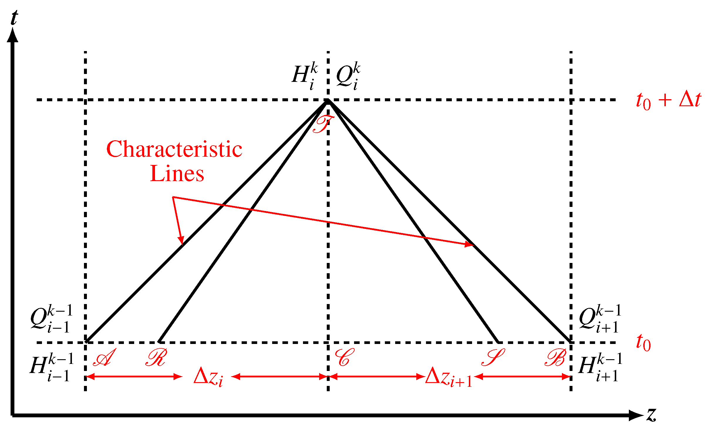
A closed-form solution for those quasi-linear hyperbolic partial differential Equations (1) and (2) is not available in general, but only for some specific boundary conditions. However, several numerical-approximation-based methods have been developed as the well-known method of characteristics (MOC) which is one of the most frequently used due to its suitability for a numerical implementation in a computer (see [12,13,17], for more details). By applying this method, an approximate solution can be carried out via a discrete integration at any point ( k , i ) discretizing the pipe according to the scheme shown in Figure 1.
Thus, after applying the MOC method through the characteristic line (Figure 2), a couple of equations, namely characteristic equations, are obtained as follows:
Along the positive characteristic line AP
Q i k = C p C a H i k
Along the negative characteristic line BP
Q i k = C n C a H i k
Needless to say, Equations (3) and (4) can be solved together. In their a posteriori representation:
A posteriori head equation:
H i k = C p C n 2 C a
A posteriori flow equation:
Q i k = C p + C n 2
where:
C p = Q i 1 k 1 + g A ϕ b H i 1 k 1 μ i 1 Δ t Q i 1 k 1 Q i 1 k 1 C n = Q i + 1 k 1 g A ϕ b H i + 1 k 1 μ i + 1 Δ t Q i + 1 k 1 Q i + 1 k 1
and:
C a = g A ϕ b

2.2.1. Convergence and Stability Conditions

Following a procedure developed in [18], it can be shown that the stability of Equations (3) and (4) is satisfied when Δ z = b Δ t (Courant condition). It implies that the characteristic line through T in Figure 2 must intersect the line AC between A and C and between C and B . For a single pipe, the computational time interval and spatial grid spacing can be selected in such a way that this condition is satisfied. However, this situation is hard to reach if the system has more than one pipe (i.e., branched pipeline system). Since it is advantageous to compute with specified time and space intervals, the following linear interpolation may be used (see Figure 2):
Q R i 1 k 1 = Q i k 1 b Δ t Δ z i Q i k 1 Q i 1 k 1 Q S i + 1 k 1 = Q i k 1 b Δ t Δ z i + 1 Q i k 1 Q i + 1 k 1 H R i 1 k 1 = H i k 1 b Δ t Δ z i H i k 1 H i 1 k 1 H S i + 1 k 1 = H i k 1 b Δ t Δ z i + 1 H i k 1 H i + 1 k 1
The values of H i k and Q i k may now be determined from Equations (3) and (4) by replacing H i 1 k 1 and Q i 1 k 1 ( H i + 1 k 1 and Q i + 1 k 1 ) by H R i 1 k 1 and Q R i 1 k 1 ( H S i + 1 k 1 and Q S i + 1 k 1 ). This is due to the characteristics through T now pass through R and S instead of through A and B , respectively. More information can be found in [12]. Thus, the Courant condition can be fixed using the smallest branch, Δ z , in a branched pipe system ensuring, that every point R and S fall inside the characteristic lines. It should be noted that such an interpolation presented by Equation (9) causes attenuation and dispersion of steep waves speeds, so, spurious waves could be generated at each boundary resulting in a slight error in the model (more information can be found in [12]). However, such an modeling error is minimized in the branch identification process due to the nature of the discrete time extended Kalman filter design, as described in Section 3.2.2 later on.

2.2.2. Special Boundary Conditions

The solution of the governing Equations (1) and (2) by using the MOC method are fully defined by a related pair of initial and boundary conditions. Such conditions describe a special relationship that defines the head and the discharge at this point. Without loss of generality, these conditions can describe a complete branched pipeline system. The algorithm presented in Section 3 is also applicable if more complex boundary conditions are needed (see [12]).

2.3. Discrete Time Extended Kalman Filter

The EKF is an algorithm for estimating unmeasured states of nonlinear dynamical systems in discrete-time considering additive uncertainties:
X k = F ( X k 1 , U k ) + W k
Y k = C X k + V k
where W k and V k are disturbance and measurement noise, respectively. The EKF is designed to minimize the covariance of the estimation error and is implemented in the following form [19,20]:
X ^ k = X ^ k + K k Y k C X ^ k
where X ^ k = F ( X k 1 , U k ) is the a priori estimate, and  X ^ k is the a posteriori estimate obtained by adding a correction term including the Kalman gain K k and the error between the measurements Y k and their estimation.

2.4. Genetic Algorithms

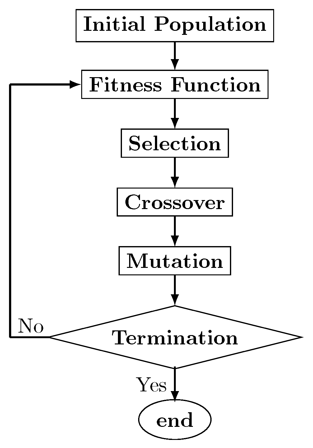
Genetic algorithms (GAs) are a type of heuristic optimization approach useful for solving non-convex optimization problems [21]. The heuristic GA search method is inspired by the theory of natural evolution. GA uses a recursive methodology to find a value (or some values) which match, exactly or approximately to a solution (solutions) in optimization and search problems [21]. Six phases are considered in a generic algorithm as shown in Figure 3 (more information can be found in [22,23]). The recursive process is repeated until a termination condition has been reached (namely termination in Figure 3). Common termination conditions include minimum criteria (a solution is found that satisfies minimum stopping criteria), allocated budget (computation time) reached, etc.
In this paper, GA will be used to find leaks in WDNs with complex branched pipeline topology. The searching process for finding the leak location could be difficult (or even impossible in some cases because of observability issues) via model-based algorithms based on a single observer that have been designed to try to locate the leak in the exact branch. On the other hand, if a bank of observers is designed to localize the position of the leak, a large computational effort could be necessary due to the high number of branches in the system. Therefore, the authors propose to reduce the number of observers in the bank and to implement a genetic algorithm to optimize the LDI process (more details are provided in Section 3).

3. LDI Scheme in a Branched Pipeline WDN

The LDI process is the task of determining if the WDN is working under a leak (i.e., leak detection) and, finding its location once it has been detected (i.e., leak isolation) [24,25]. However, for branched pipeline WDNs, the LDI problem could be a challenging task in case of complex and large scale case studies.

3.1. General Branched Pipeline LDI System Design Principles

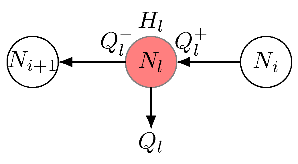
Without loss of generality and for the sake of simplicity, a general branched pipeline can be modeled with just three types of nodes: input, inner and output nodes. Input nodes represent the upstream inputs of the system, (Figure 4c) (input measurement). In the same way, inner nodes correspond to the branching junction of several pipes (Figure 4b). Finally, output nodes characterize the downstream outputs of the system (Figure 4a). Each node is related to a vector which is built by the flow-rate and the pressure head corresponding to such a node, as Figure 4 shows. Notice that, in the inner node, three flow rates are considered: Q i + 1 denotes the flow-rate between the nodes N i and N i + 1 ; Q i + 1 is the flow-rate between the nodes N i + 1 and N i + 2 ; and, finally, Q i + 1 denotes the flow-rate between the nodes N i + 1 and N i + 3 . These variables are related with the equation at the boundary condition corresponding to a “branching junction” in the MOC. For the output nodes, the downstream valve boundary condition could be the most suitable for its characterization (see [12]). Here, the relative valve opening is fixed since orifice opening remains constant over the transient response.
To complete the whole LDI system design, the characterization of a leak in a particular branch should be carried out. This can be done following a similar idea as for the inner nodes presented above (Figure 4), but under certain considerations (see Figure 5): Note that the leak flow influence is additive (because of the mass conservation law). That is, the flow rate before the leak Q l + must be equal to the sum of the flow rate after the leak, Q l plus the flow through the leak hole, that is Q l + = Q l + Q l (Figure 5). Thus, the boundary condition equation for a leak node in Figure 5 following the branching junction derivation yields:
H l = C p l C n l Q l 2 C a Q l + = C p l C a H l Q l = C n l C a H l
where C p l and C n l are defined through the characteristic line. Noticed that subscripts p l and n l denote the point before and after the leak, respectively. Moreover, in Equation (7) μ i 1 = μ i + 1 = μ l and Q l is computed as in (16), see [12]. It is worth noting that in Equation (9) Δ z i = z f while Δ z i + 1 = z i z f ( z i is the distance between the i-th and ( i + 1 ) -th node where the leak is located).
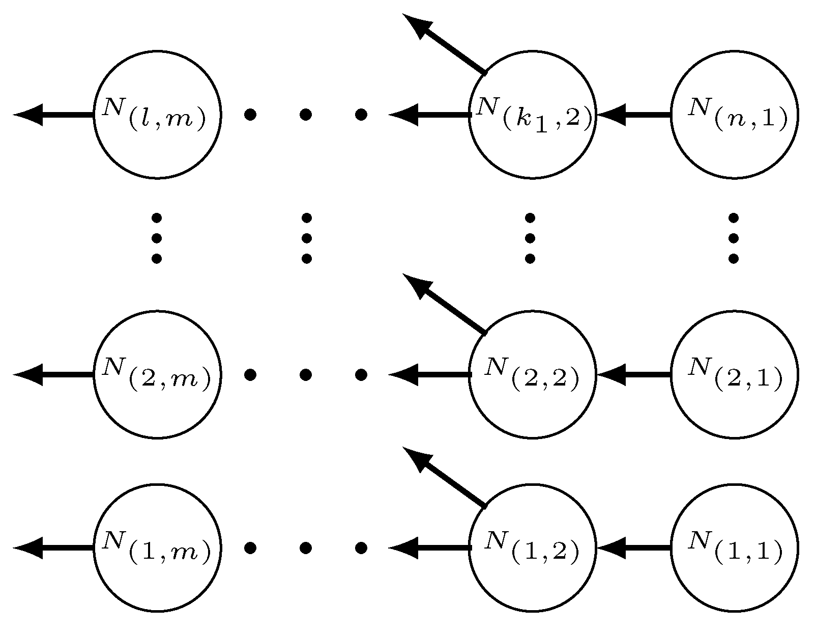
As outlined above, the present approach assumes only flow and pressure sensors at the input (upstream) and output (downstream) nodes. Thus, the flow-rate and the pressure head at the input nodes will be considered as the system entries, whereas the output node measurements will be the system outputs. Thus, a branched pipeline system can be characterized as individual units (nodes). Figure 6 shows a general scheme architecture built by n inputs nodes, m 2 layers of inner nodes and l outputs nodes. Here, each k i denotes the number of nodes at the i-th inner layer.
Now, each flow-rate and pressure head can be computed using Equations (5), (6), (9) and (13), together with its respective boundary conditions. Proceeding in this way, the pipeline system architecture shown in Figure 6 can be modelled using a difference equation system as follows:
X k = F ( X k 1 , U k )
Y k = C X k
where:
X = H 1 , Q 1 , Q 1 , Q 1 , , H p , Q p , Q p , Q p , H l , Q l + , Q l , H o u t 1 , Q o u t 1 , , H o u t o , Q o u t o T U = H i n 1 , Q i n 1 , , H i n q , Q i n q T C =   0 2 o × ( 4 p + 3 )   |   I 2 o  
where the subscript q, p and o denote the number of inputs, inner and output nodes, respectively.

3.2. Leak Detection and Isolation Process

In this work, the authors propose three phases for the LDI process: leak detection, branch identification and leak isolation. Leak detection aims at detecting when the leak appears in the system; branch identification consists in establishing the nodes among which the leak is located; and, lastly, leak isolation consists in determining the distance between the inner node of the fixed branch in a previous phase and leak position. More details of these processes are explained in the following.

3.2.1. Leak Detection

Considering the mass conservation law, the flow-rate through a leak hole, Q l , can be calculated using the following relationship [26]:
Q l = q Q i n q Q o u t
Thus, the leak can be detected using the simple mass balance (16) altogether with a threshold δ establishing the leak condition as follows: | Q l | > δ . This threshold should be defined experimentally according to the noise in the measurements (as e.g.,  δ must be at least larger than a number of times the variance of the difference between Q i n Q o u t to avoid false alarms). Moreover, the calculation of Q l will be used in the isolation process as discussed below.

3.2.2. Branch Identification

If a leak occurs, an alarm is triggered when | Q l | > δ . Other kind of alarms can be found in [27]. At this point, the GA-based branch identification algorithm following the principles presented in Section 2.4 is started. To do that, the size of phenotype (population) must be defined by the designer considering the computational effort and according to the number of branches. Such a population is a subset of the natural number set N limited up to the number of branches in the pipeline as follows:
P Q = { 1 , 2 , , n o }
where Q stands for the search space, n o is the number of branches. It should be noted that the population is taken randomly from Q .
The branch identification process is done via an implementation of n o = P (the cardinality of the set P ) EKFs by using (12) for a system description given by (14) which allows the estimation error to be minimized. Such observer only differ in the position of the leak variables, H l , Q l + and Q l , in Equation (14), preserving the order of the branch in question given by a number in P (i.e., for a number i P , the leak node is induced at position l i / 2 of the corresponding branch).
Fitness function. The bank of EKFs is used to generate a residual vector defined as r ( t ) = r 1 ( t ) ,   r 2 ( t ) ,   ,   r o ( t ) T . Each residual r i ( t ) is the difference between the observer output flows and the measured output flows normalized with respect to the real (measured) flows:
r i ( t ) = Q i ( t ) Q ^ i ( t ) Q i ( t )
where Q i and Q ^ i stand for the flow-rate, measured and estimated in the i-th output node, respectively. This normalization is used because of the possible differences between output flows allowing the residuals to be comparable in [ 0 , 1 ] scale.
GA-based algorithm aims at finding the leaking-branch (each of them characterized by an observer) based on finding leak location that minimizes the L 2 -norm residual (i.e., the lowest energy observer) as in [28]:
min t 0 t 0 + T w r ( t ) T r ( t )   d t
where T w is a time window.
Once the winning population is found, a new set of phenotypes is randomly generated to replace the ones that have not survived and thus, to complete the whole population for the new iteration (in other words, a new set of branch number, that has not already been tried, is selected randomly). If no new population is generated, the termination conditions are achieved.

3.2.3. Leak Isolation

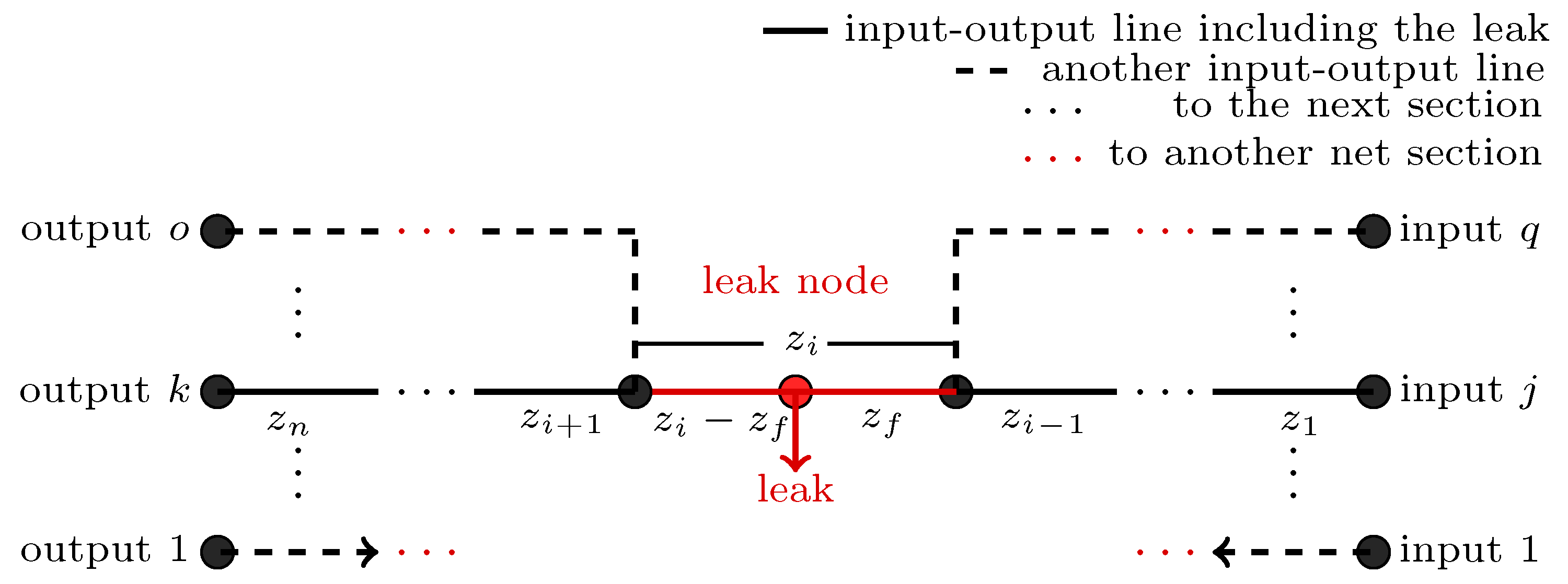
The last step of the LDI process is to estimate the distance between the upstream node of the winner branch and the leak point z ^ f , see Figure 7. As it can be seen, the input-output pipe sections that include the leak node are shown with dashed line (input q to output o). Those input-output that do not pass through to the leak node are denoted by dashed lines (input and output number 1). The process to isolate the leak is carry out taken any input-output pipeline that contains the leak node (for example input j to output k, solid line). Then, let us consider that it is possible to compute the pressure drop between two consecutive nodes using Equation (1) in steady state, i.e.,  Q ( t , z ) t = 0 and H ( t , z ) z = H n + H n z n , it yields:
H n + H n = z n μ n g A ϕ Q n 2
where H n + and H n denote the measured pressures at the previous and posterior nodes, respectively; Q n is the flow-rate, μ n is computed as in Equation (1) and z n is the distance through the analyzed section. Now, following the scheme depicted in Figure 7, it is possible to take any input-output branch (input j to output k, for instance) and using (20) it is possible to compute the pressure drop in all inner nodes. By hypothesis, the measurements of the inner nodes are not available, but, it is possible to sum recursively the result given by Equation (20) through the whole pipe-section under study (note that H n appears with negative sign in the first section but with positive sign in the next section, such that if (20) is summed recursively, the inner pressure measurements disappear). After some algebraic manipulations it results in:
z ^ f = H i n j H o u t k i = 1 n μ i z i Q i 2 μ l ( ( Q l + ) 2 ( Q l ) 2 )
where H i n j and H o u t k are the pressure head at upstream and downstream, respectively, in the considered branch (see Figure 7); μ i and μ l are the constant μ (as in Equation (1)) but being μ l computed with the friction factor in the branch where the leak is induced; Q i the flow-rate in the i-th pipe in the network; and z i the distance of the pipe between the i-th and the ( i + 1 ) -th node. Finally, Q i + and Q i is the flow-rate before and after the leak location, respectively (see Figure 5). It is worth pointing out that in the summation in Equation (21), if i is the leaky branch, then Q i = Q i and Q i + and Q i can be computed indirectly through the measured flows by means of a mass valance. Finally, note that in steady state, z ^ f is computed using the pressure drop between any input and output nodes since it must be equal to the pressure drop as a result of the flow rate in each branch following the Darcy-Weisbach equation being its advantage over other methods [15,29].

3.2.4. LDI Pseudo Code

The following pseudo code summarizes the implementation of the proposed LDI algorithm (Algorithm 1):
Algorithm 1 LDI Scheme
1:
while true do
2:
      Q i n 1 , 2 , . . . , q R e a d F l o w S e n s o r s ( )
3:
      H i n 1 , 2 , . . . , q R e a d P r e s s u r e S e n s o r s ( )
4:
      Q l = q Q i n q Q o u t
5:
     if  | Q l | > δ  then
6:
        P ← Take randomly n o elements in Q (initial population)
7:
       while true do
8:
          for  i = 1 , , n o  do
9:
               r i Run observer T w second inducing the leak in the j-th branch ( j P )
10:
        end for
11:
        Take the best elements that fulfill Equation (19)
12:
        Remove the worst elements from Q
13:
        Complete P taking the rest element randomly from Q
14:
        if  P = Q  then
15:
            break
16:
        end if
17:
     end while
18:
   end if
19:
   if  P = Q  then
20:
     break
21:
   end if
22:
end while
23:
Compute z ^ f from Equation (21)
24:
return  z ^ f

4. Tuxtla Gutiérrez Pilot Plant: A Case Study

To evaluate the performance of the proposed LDI scheme, experimental results are presented in this section. The experiments are carried out using several databases from the pilot plant built at the Hydraulics Laboratory of the National Technological Institute of Mexico (TecNM) in Tuxtla Gutiérrez, Chiapas. A general description of the pipeline prototype is presented below. Then, the pilot plant modeling and the application of the LDI is presented. Finally, experiments for all possible leak scenarios are successfully solved and discussed.

4.1. Pilot Pipeline Description

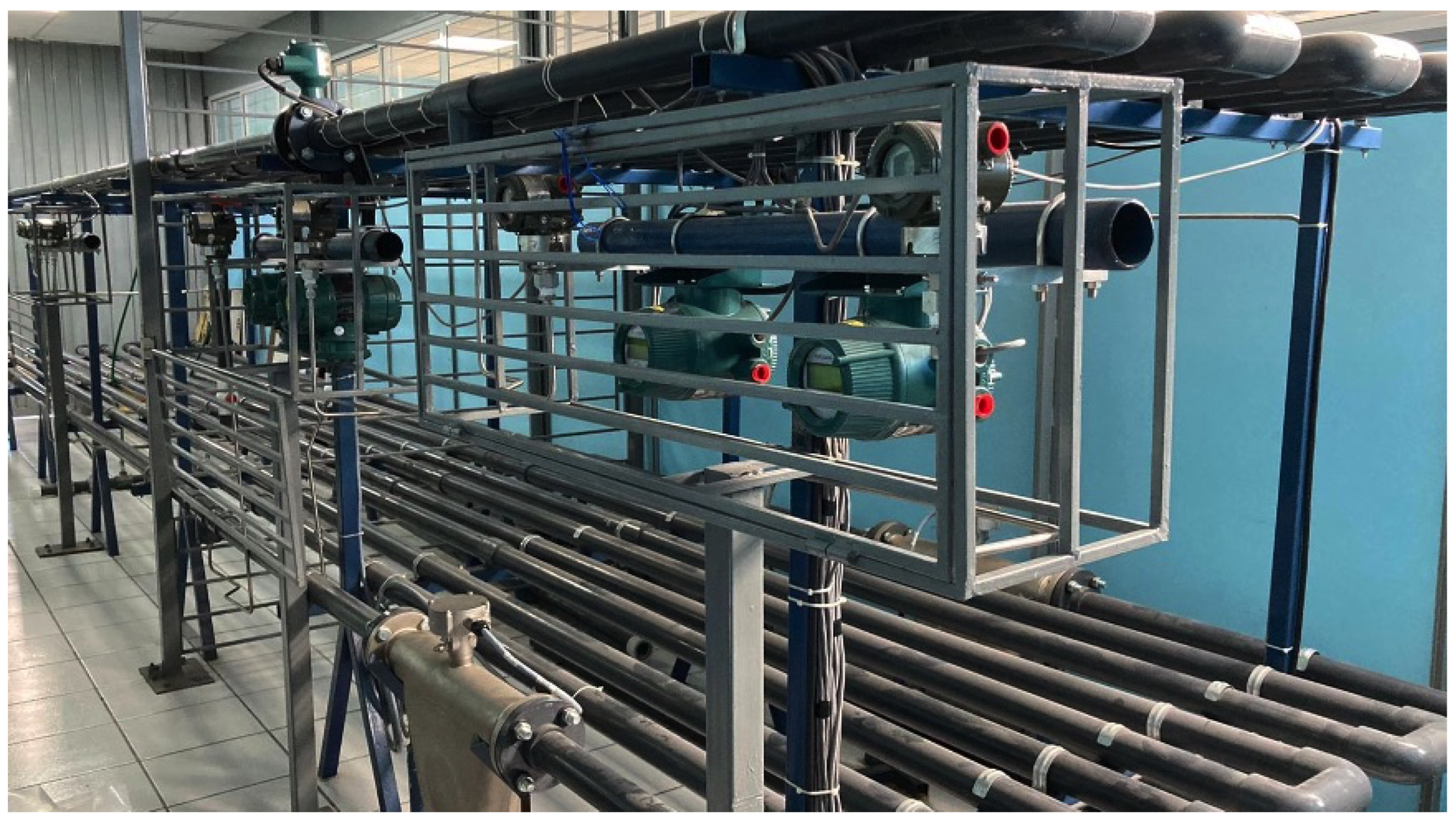
The layout of the pilot plant is depicted in Figure 8 and Figure 9. This pilot plant is composed by one main line and a couple of branches connected to it. This configuration has five pipe sections. In each pipe section, a valve is installed and it can be opened to create a leak scenario, see Figure 8. A 5 [HP] hydraulic pump impulses the water through the system which is made of Polyvinyl Chloride (PVC) with an inner diameter of 4.86 [cm] (approx. two inches). A variable-frequency drive to regulate the pressure head is also included. A 2.5 [m 3 ] reservoir is placed upstream and another is placed downstream to recirculate the water.
Moreover, flow-rate sensors are placed upstream and also at all delivery points (downstream); pressure head sensors are installed at both upstream and downstream but also at the branching connections. It should be noted that those pressure heads at branching connections are not used by the LDI system but are only used for validation purposes. The main pipeline parameters are shown in Table 1 (see [30] for more information).

4.2. Pilot Plant Modeling

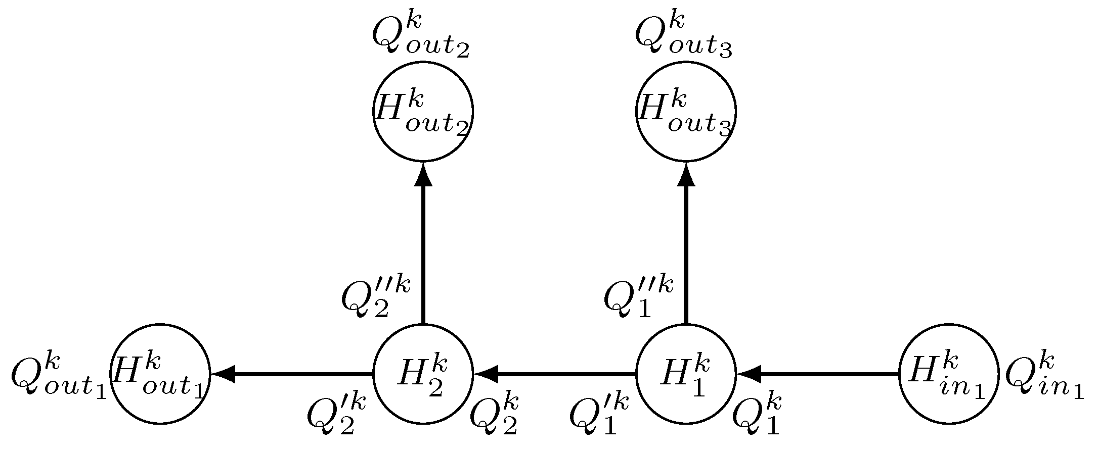
Applying the proposed architecture to the Tuxtla Gutiérrez Pilot Plant (Section 3.1) yields to the scheme depicted in Figure 10. As it can be seen, it has one input node [ H 1   Q 1 ] T , two inner nodes [ H 2   Q 2   Q 2   Q 2 ] T and [ H 3   Q 3   Q 3   Q 3 ] T and three output nodes [ H 4   Q 4 ] T , [ H 5   Q 5 ] T and [ H 6   Q 6 ] T .
Considering q = 1 , p = 2 and o = 3 in Equation (14) leads to the following state-space representation:
X = H 1 , Q 1 , Q 1 , Q 1 , H 2 , Q 2 , Q 2 , Q 2 , H l , Q l + , Q l , H o u t 1 , Q o u t 1 , H o u t 2 , Q o u t 2 , H o u t 3 , Q o u t 3 T
U = H i n 1 , Q i n 1 T
C =   0 6 × 11   |   I 6  
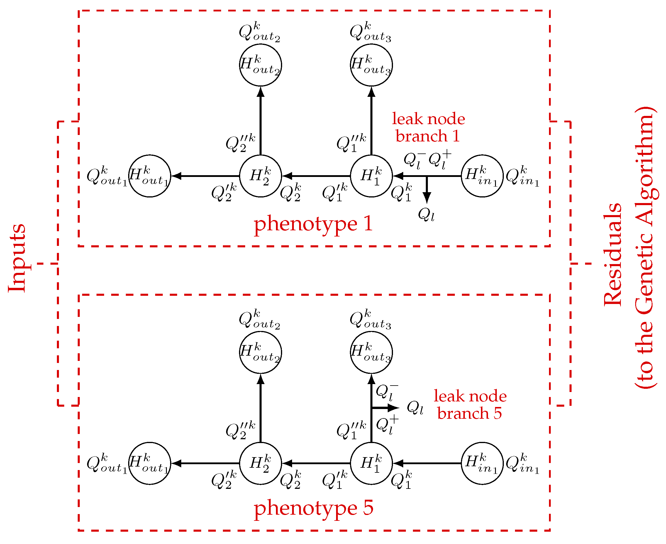
Thus, if two phenotypes are selected, two observers must be built. In this example, the number of branches is limited, therefore, an observer in each ramification can be built. However, in a real case, where the number of branches are significant, a reduced observer can be built. Each observer can seek for the leaking-branch (phenotypes in the GA). In this way, computational effort can be reduced. Figure 11 shows two observers fighting for the lowest residual (Fitness Function in Equation (19)). Obviously, here the phenotypes are 1 and 5 respectively.
The observers are designed using the state-space representation, Equation (14) and EKF approach described in Section 2.3.

4.3. Experimental Results

Five experiments are performed using several databases from the pilot plant described in Section 4.1. The experiment was carried out under the same conditions: to emulate a leak, the opening of one of the valves numbered from one to five (see Figure 8), respectively, is carried out approximately ten seconds after the experiment begins. The algorithm is started once the leak is detected via a mass balance approach as discussed in Section 3.2.1. Immediately afterwards, the GA-based algorithm described in Section 2.4 is executed.
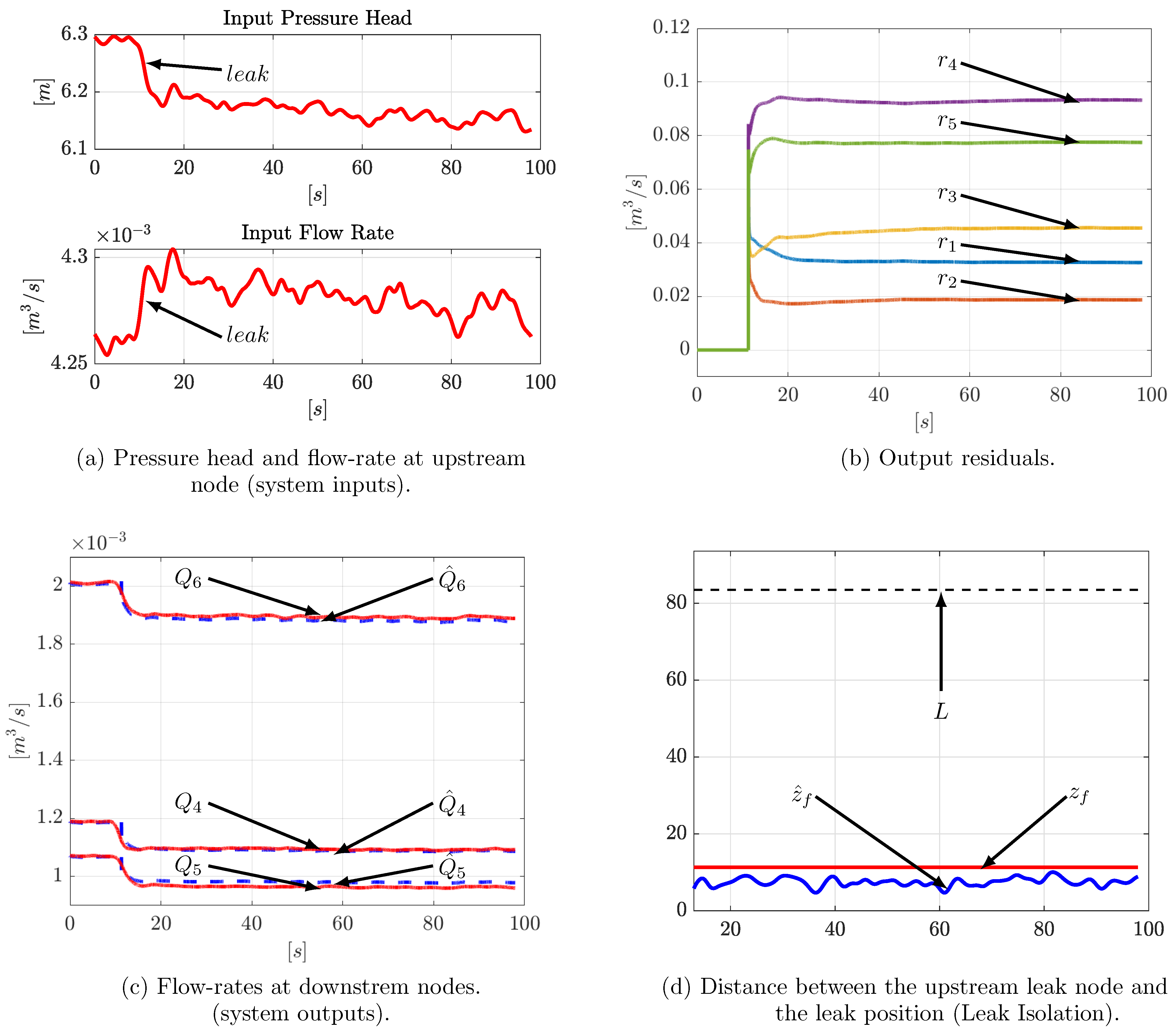
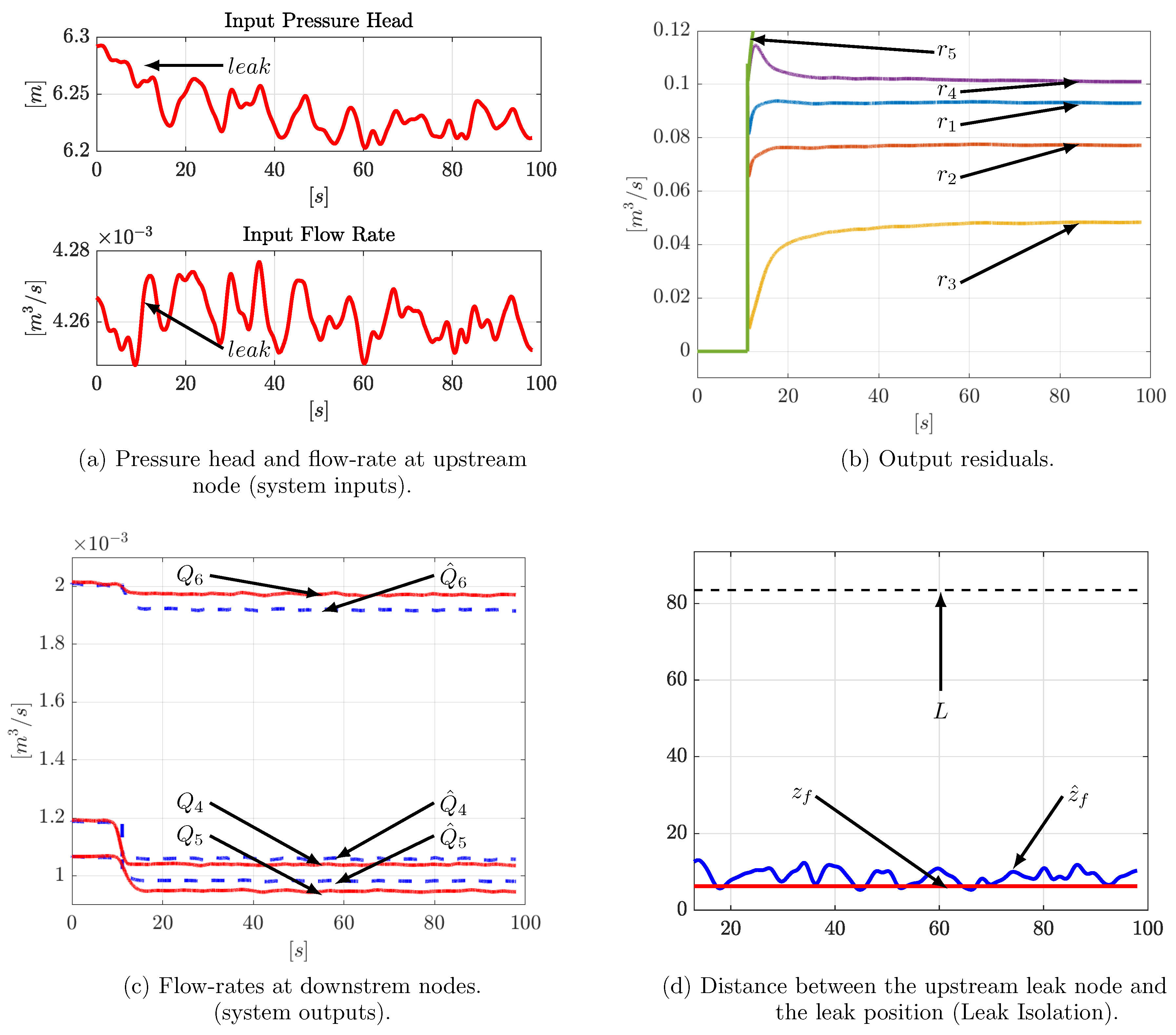
Figure 12, Figure 13, Figure 14, Figure 15 and Figure 16 show the results regarding experiments based on creating leaks from valves one to five, respectively. Figure 12a, Figure 13a, Figure 14a, Figure 15a and Figure 16a depict the dynamic of the flow-rate and the pressure head at the upstream node (input variables).
As previously mentioned (Section 4.2), two phenotypes are used in this application. However, for demonstration purposes, Figure 12b, Figure 13b, Figure 14b, Figure 15b and Figure 16b depict the residuals of the five observers (one for each branch of the system) once the GA has converged. Note that the observer that presented the minimum energy is indeed the corresponding to the leaking-branch. It should be noted that residuals were smoothed for clarity purposes.
Figure 12c, Figure 13c, Figure 14c, Figure 15c and Figure 16c depict the flow-rates outputs, observer ( Q ^ i ) and the measured one ( Q i ) of the winner observer. As it can be seen, the mathematical model follows the real data in a proper way despite the measurement noise.
Figure 12d, Figure 13d, Figure 14d, Figure 15d and Figure 16d show the distance between the upstream leak node and the leak position (leak isolation), the real one z f (concerning) and its estimation z ^ f . As shown, the leak position is well estimated. In the same figure, the length of the whole input-output branch where the leak is located, L is shown. The latter is performed to illustrate the gap between the real leak distance and its estimation.
Finally, for the sake of comparison the classical extended Kalman filter designed as in [7] is also implemented and its results are then compared with those obtained in this paper. In Table 2 this comparison is summarized. As it can be seen, the GA approach outperforms the classical extended Kalman filter (EKF) in two experiments whereas the classic EKF is better in one experiment. Certainly, these results are obtained using a test bed pilot plant and the following step is to evaluate the performance of the GA approach in a real-life leak scenario to then compare it with the EKF which has already been implemented to solve a real life leak problem [31].

4.4. Some Final Remarks

(1)
The algorithm can hardly identify the parameters of a leak with a rate greater than 10 % of the nominal flow since this event can be considered as a catastrophic failure instead of a simple fault, this is because the assumptions to obtain a modeling of the system could not be fulfilled correctly. Moreover the smallest leak that can be detected depends directly on the accuracy of the flow rate sensors (noise variance).
(2)
To obtain moving average values of the input and output measurements, they are filtered with the equation [31]:
ς F ( k ) = 1 2 N + 1 ( ς ( K + N ) + ς ( k + N 1 ) + . . . + ς ( k N ) )
where ς F ( k ) is the smoothed value for the signal ς ( ) at time k, N is the number of neighboring data taken on either side of ς F ( k ) , and 2 N + 1 is the span dimension.
(3)
The initial conditions of the observer, X 0 are fixed as follows: H 4 0 , Q 4 0 , H 5 0 , Q 5 0 , H 6 0 and Q 6 0 are equal to the mean values of the measured outputs in a steady-state leak-free condition.
(4)
The inner pressure initial conditions (i.e., H 2 0 , H 3 0 ) are calculated using the well-know Darcy-Weisbach friction equation [15,29]:
H i 0 = H i 1 0 μ i z i Q i 0 2
where i = { 2 , 3 } .
(5)
On the other hand, the inner flow-rate initial conditions. Q 2 0 , Q 2 0 , Q 2 0 , Q 3 0 , Q 3 0 , Q 3 0 , are computed using the law of conservation of mass:
Q i 0 = Q i 0 + Q i 0
where, as before, i = { 2 , 3 } . Moreover, due to the same law and in steady-state conditions, the next relationships must be satisfied: Q 3 0 = Q 4 0 , Q 3 0 = Q 5 0 , Q 2 0 = Q 6 0 and Q 2 0 = Q 3 0 (see Figure 10).
(6)
As is well known, the friction factor, τ in Equation (1), radically changes with the flow velocity in smooth pipes (pipes with a relative roughness usually lower than 1 × 10 3 ). That is why in the present work, the friction factor is calculated by using the Swamee-Jain [15]:
τ ( Q ) = 0.25 log 10 ϵ r 3.7 + 5.74 Re 0.9 2
It is worth noting that it is not necessary to update the friction factor once the leak appears, since its size by hypothesis is lower than 10% of the nominal flow rate in a steady-state (see point (1)). The friction factors are shown in Table 3.

5. Conclusions and Future Work

The present work deals with the real-time leak detection and isolation problem in branched pipeline systems present in many real water distribution networks. The approach has been split into three main stages: leak detection, branch isolation and leak location. The scheme only assumes flow and pressure sensors at the beginning and the end of the system.
The first point to underline is that in complex water distribution systems, the leak location problem could be difficult to solve due to the high number of nodes (branches) in the system. That is why the authors propose a genetic based algorithm together with a bank of observer which aims to isolate the leaking branch by reducing the computational effort.
The leak location was carried out using the pressure drop between an input and an output node of the branch in question and the flow-rate through it.
The approach estimated the leaking branch accurately and the leak position in a very acceptable way. The use of a integration error as a fitness function, altogether with the Kalman filter, helped obtain a good estimation despite the presence of noise.
As a future work, three paths will be addressed: (i) the proposed approach will be refined to achieve better performance; (ii) the authors will explore the possibility of extending the approach to locate two leaks; (iii) the algorithm will be tested to locate leaks in a real water distribution network.

Author Contributions

Conceptualization, A.N.-D. and J.A.D.-A.; methodology, A.N.-D. and J.A.D.-A.; software, A.N.-D.; validation, A.N.-D., J.A.D.-A., I.S.-R. and V.P.; formal analysis, I.S.-R. and V.P.; investigation, A.N.-D. and J.A.D.-A.; resources, A.N.-D., J.A.D.-A. and I.S.-R.; data curation, I.S.-R.; writing—original draft preparation, A.N.-D. and J.A.D.-A.; writing—review and editing, I.S.-R. and V.P.; visualization, J.A.D.-A. and V.P.; supervision, A.N.-D.; funding acquisition, A.N.-D. and I.S.-R. All authors have read and agreed to the published version of the manuscript.

Funding

The APC was funded by Tecnológico de Monterrey. The experimental work was supported in part by Tecnológico Nacional de México (TecNM) under grant 14515.22-P.

Institutional Review Board Statement

Not applicable.

Informed Consent Statement

Not applicable.

Data Availability Statement

Not applicable.

Conflicts of Interest

The authors declare no conflict of interest.

References

  1. OECD. Water Governance in Cities; OECD Studies on Water; OECD Publishing: Paris, France, 2016; p. 140. [Google Scholar] [CrossRef]
  2. Santos-Ruiz, I.; López-Estrada, F.R.; Puig, V.; Valencia-Palomo, G.; Hernández, H.R. Pressure Sensor Placement for Leak Localization in Water Distribution Networks Using Information Theory. Sensors 2022, 22, 443. [Google Scholar] [CrossRef] [PubMed]
  3. Morales-González, I.O.; Santos-Ruiz, I.; López-Estrada, F.R.; Puig, V. Pressure Sensor Placement for Leak Localization Using Simulated Annealing with Hyperparameter Optimization. In Proceedings of the 2021 5th International Conference on Control and Fault-Tolerant Systems (SysTol), Saint-Raphaël, France, 29–30 September 2021; pp. 205–210. [Google Scholar] [CrossRef]
  4. Perez, R.; Sanz, G.; Puig, V.; Quevedo, J.; Cuguero Escofet, M.A.; Nejjari, F.; Meseguer, J.; Cembrano, G.; Mirats Tur, J.M.; Sarrate, R. Leak Localization in Water Networks: A Model-Based Methodology Using Pressure Sensors Applied to a Real Network in Barcelona [Applications of Control]. IEEE Control Syst. Mag. 2014, 34, 24–36. [Google Scholar] [CrossRef] [Green Version]
  5. Levinas, D.; Perelman, G.; Ostfeld, A. Water Leak Localization Using High-Resolution Pressure Sensors. Water 2021, 13, 591. [Google Scholar] [CrossRef]
  6. Sun, C.; Parellada, B.; Puig, V.; Cembrano, G. Leak Localization in Water Distribution Networks Using Pressure and Data-Driven Classifier Approach. Water 2020, 12, 54. [Google Scholar] [CrossRef] [Green Version]
  7. Delgado-Aguiñaga, J.; Besançon, G. EKF-based leak diagnosis schemes for pipeline networks. IFAC-PapersOnLine 2018, 51, 723–729. [Google Scholar] [CrossRef]
  8. Torres, L.; Verde, C.; Molina, L. Leak diagnosis for pipelines with multiple branches based on model similarity. J. Process Control 2021, 99, 41–53. [Google Scholar] [CrossRef]
  9. Delgado-Aguiñaga, J.; Santos-Ruiz, I.; Besançon, G.; López-Estrada, F.; Puig, V. EKF-based observers for multi-leak diagnosis in branched pipeline systems. Mech. Syst. Signal Process. 2022, 178, 109198. [Google Scholar] [CrossRef]
  10. Pan, B.; Capponi, C.; Meniconi, S.; Brunone, B.; Duan, H.F. Efficient leak detection in single and branched polymeric pipeline systems by transient wave analysis. Mech. Syst. Signal Process. 2022, 162, 108084. [Google Scholar] [CrossRef]
  11. Liao, Z.; Yan, H.; Tang, Z.; Chu, X.; Tao, T. Deep learning identifies leak in water pipeline system using transient frequency response. Process Saf. Environ. Prot. 2021, 155, 355–365. [Google Scholar] [CrossRef]
  12. Chaudhry, M.H. Transient-flow equations. In Applied Hydraulic Transients; Springer: Berlin/Heidelberg, Germany, 2014; pp. 35–64. [Google Scholar]
  13. Streeter, V.L.; Lai, C. Water-hammer analysis including fluid friction. Trans. Am. Soc. Civ. Eng. 1963, 128, 1491–1524. [Google Scholar] [CrossRef]
  14. Srbislava, G.; Ivana, A.; Petara, K.; Markob, J.; Nikolab, B.; Vojislavc, G. A review of explicit approximations of Colebrook’s equation. FME Trans. 2011, 39, 67–71. [Google Scholar]
  15. Abdulameer, L.S.; Dzhumagulova, N.; Algretawee, H.; Zhuravleva, L.; Alshammari, M.H. Comparison between Hazen-Williams and Darcy-Weisbach Equations to Calculate Head Loss through Conveyancing Treated Wastewater in Kerbala City, Iraq. East.-Eur. J. Enterp. Technol. 2022, 1, 115. [Google Scholar] [CrossRef]
  16. Dulhoste, J.F.; Besançon, G.; Ortiz, F.L.T.; Begovich, O.; Navarro, A. About friction modeling for observer-based leak estimation in pipelines. In Proceedings of the 2011 50th IEEE Conference on Decision and Control and European Control Conference, Orlando, FL, USA, 12–15 December 2011; pp. 4413–4418. [Google Scholar]
  17. Carlsson, J. Water Hammer Phenomenon Analysis Using the Method of Characteristics and Direct Measurements Using a “Stripped” Electromagnetic Flow Meter. Master’s Thesis, Royal Institute of Technology, Stockholm, Sweden, 2016. [Google Scholar]
  18. O’Brien, G.G.; Hyman, M.A.; Kaplan, S. A Study of the Numerical Solution of Partial Differential Equations. J. Math. Phys. 1950, 29, 223–251. [Google Scholar] [CrossRef]
  19. Simon, D. Optimal State Estimation: Kalman, H Infinity, and Nonlinear Approaches; John Wiley & Sons: Hoboken, NJ, USA, 2006. [Google Scholar]
  20. Fujii, K.; The ACDA-Sim-J Group. Extended Kalman Filter. Reference Manual. 2013, pp. 14–22. Available online: https://www-jlc.kek.jp/2004sep/subg/offl/kaltest/doc/ReferenceManual.pdf (accessed on 3 May 2022).
  21. Katoch, S.; Chauhan, S.S.; Kumar, V. A review on genetic algorithm: Past, present, and future. Multimed. Tools Appl. 2021, 80, 8091–8126. [Google Scholar] [CrossRef] [PubMed]
  22. Kumar, M.; Husain, M.; Upreti, N.; Gupta, D. Genetic Algorithm: Review and Application (1 December 2010). Available online: https://ssrn.com/abstract=3529843 (accessed on 16 April 2022).
  23. Mathew, T.V. Genetic Algorithm. Report Submitted at IIT Bombay 2012. Indian Institute of Technology, Bombay, Mumbai. Available online: http://datajobstest.com/data-science-repo/Genetic-Algorithm-Guide-[Tom-Mathew].pdf (accessed on 16 April 2022).
  24. Isermann, R. Fault-Diagnosis Systems: An Introduction from Fault Detection to Fault Tolerance; Springer: Berlin/Heidelberg, Germany, 2005. [Google Scholar]
  25. Gertler, J.J. Fault Detection and Diagnosis in Engineering Systems; CRC Press: Boca Raton, FL, USA, 2017. [Google Scholar]
  26. Boaz, L.; Kaijage, S.; Sinde, R. An overview of pipeline leak detection and location systems. In Proceedings of the 2nd Pan African International Conference on Science, Computing and Telecommunications (PACT 2014), Arusha, Tanzania, 14–18 July 2014; pp. 133–137. [Google Scholar]
  27. Soldevila, A.; Boracchi, G.; Roveri, M.; Tornil-Sin, S.; Puig, V. Leak detection and localization in water distribution networks by combining expert knowledge and data-driven models. Neural Comput. Appl. 2022, 34, 4759–4779. [Google Scholar] [CrossRef]
  28. Navarro, A.; Delgado-Aguiñaga, J.A.; Sánchez-Torres, J.D.; Begovich, O.; Besançon, G. Evolutionary Observer Ensemble for Leak Diagnosis in Water Pipelines. Processes 2019, 7, 913. [Google Scholar] [CrossRef] [Green Version]
  29. Lindstrom, L.; Gracy, S.; Magnusson, S.; Sandberg, H. Leakage Localization in Water Distribution Networks: A Model-Based Approach. arXiv 2022, arXiv:2204.00050. [Google Scholar]
  30. Santos-Ruiz, I.; Bermúdez, J.; López-Estrada, F.; Puig, V.; Torres, L.; Delgado-Aguiñaga, J. Online leak diagnosis in pipelines using an EKF-based and steady-state mixed approach. Control Eng. Pract. 2018, 81, 55–64. [Google Scholar] [CrossRef]
  31. Delgado-Aguiñaga, J.; Begovich, O. Water leak diagnosis in pressurized pipelines: A real case study. In Modeling and Monitoring of Pipelines and Networks; Verde, C., Torres, L., Eds.; Springer International Publishing: Berlin/Heidelberg, Germany, 2017; pp. 235–262. [Google Scholar]
Figure 1. Pipeline discretization using the MOC.
Water 14 03289 g001
Figure 2. MOC-based discretization scheme.
Water 14 03289 g002
Figure 3. Genetic algorithm scheme.
Water 14 03289 g003
Figure 4. Atomic representation for an output, inner an input node. (a) Output Node; (b) Inner Node; (c) Input Node.
Water 14 03289 g004
Figure 5. Leak characterization scheme.
Water 14 03289 g005
Figure 6. General branched pipeline system architecture.
Water 14 03289 g006
Figure 7. General scheme of a water distribution net.
Water 14 03289 g007
Figure 8. Pipeline system layout.
Water 14 03289 g008
Figure 9. Pipeline prototype.
Water 14 03289 g009
Figure 10. Branched pipeline structure.
Water 14 03289 g010
Figure 11. LDI scheme.
Water 14 03289 g011
Figure 12. Experiment 1: leak induced in valve 1: (a) Pressure head and flow rate at upstream, (b) Output residuals, (c) Flow rate at downstream nodes and, (d) Leak position.
Water 14 03289 g012
Figure 13. Experiment 2: leak induced in valve two: (a) Pressure head and flow rate at upstream, (b) Output residuals, (c) Flow rate at downstream nodes and, (d) Leak position.
Water 14 03289 g013
Figure 14. Experiment 3: leak induced in valve 3: (a) Pressure head and flow rate at upstream, (b) Output residuals, (c) Flow rate at downstream nodes and, (d) Leak position.
Water 14 03289 g014
Figure 15. Experiment 4: leak induced in valve 4: (a) Pressure head and flow rate at upstream, (b) Output residuals, (c) Flow rate at downstream nodes and, (d) Leak position.
Water 14 03289 g015
Figure 16. Experiment 5: leak induced in valve 5: (a) Pressure head and flow rate at upstream, (b) Output residuals, (c) Flow rate at downstream nodes and, (d) Leak position.
Water 14 03289 g016
Table 1. Pipeline parameters.
ParameterSymbolValueDimension
Inner diameter ϕ 4.86 × 10 2 m
Wave speedb 422.75 m / s
Relative roughness ϵ r 3.47 × 10 4
Fluid kinematic viscosity ν 8.03 × 10 7 m 2 / s
Fluid density ρ 996.59 k g / m 3
Acceleration due to gravityg 9.79 m / s 2
Table 2. Error norm for each LDI approach.
Case e z l GA [m] e z l EKF [m]
Experiment 1 1.29 × 10 2 2.98 × 10 2
Experiment 2 1.53 × 10 2 4.46 × 10 2
Experiment 3 1.08 × 10 2 0.98 × 10 2
Table 3. Friction factors for each branch.
Branch NumberSymbolValue
1 τ 1 2.40 × 10 2
2 τ 2 2.68 × 10 2
3 τ 3 3.67 × 10 2
4 τ 4 5.95 × 10 2
5 τ 5 3.76 × 10 2
Publisher’s Note: MDPI stays neutral with regard to jurisdictional claims in published maps and institutional affiliations.