Article

Energy Analysis of a Quasi-Two-Dimensional Friction Model for Simulation of Transient Flows in Viscoelastic Pipes

1
State Key Laboratory of Urban Water Resource and Environment, School of Environment, Harbin Institute of Technology, Huanghe Road No. 73, Harbin 150090, China
2
School of Energy and Architecture Engineering, Harbin University of Commerce, Harbin 150028, China
3
Industrial Control Energy Saving Business Division, Beijing Huada Zhibao Electronic System Co., Ltd., Beijing 100020, China
*
Author to whom correspondence should be addressed.
Water 2022, 14(20), 3258; https://doi.org/10.3390/w14203258
Submission received: 23 August 2022 / Revised: 5 October 2022 / Accepted: 10 October 2022 / Published: 15 October 2022
(This article belongs to the Special Issue About an Important Phenomenon—Water Hammer)

Abstract

:
Quasi-two-dimensional (quasi-2D) friction models have been widely investigated in transient pipe flows. In the case of viscoelastic pipes, however, the effect of different values of the Reynolds number (Re) on pressure fluctuations (which can lead to water hammer) have not been considered in detail. This study establishes a quasi-2D friction model employing an integral total energy method and investigates the work due to frictional and viscoelastic terms at different Re values. The results show that viscoelastic work (WP) and frictional work (Df) increase with an increase in Re. However, when the initial Re values are high, the Df values are much larger than the WP values. In addition, for Re < 3 × 10⁵, the 1D model underestimated the viscoelastic terms. There was no significant difference between the two models for Re > 3 × 10⁵. In the case of different initial Re values, the two models produced almost the same values for WP. This study provides a theoretical basis for investigating transient flow from the perspective of energy analysis.

1. Introduction

In recent years, viscoelastic pipes have been increasingly used in urban water-supply systems [1]. The transient-flow pressure fluctuation generated by such pipes is different from the pressure fluctuation of traditional elastic pipes because of their different viscoelastic properties; when pumps suddenly stop or valves close quickly, a water-hammer accident result. The peak values of pressure fluctuation are relatively small; however, pressure-fluctuation attenuation and phase delay are large. Therefore, a correct understanding of the role of viscoelastic characteristics in the transient-flow pressure-fluctuation process is necessary.
Accurate numerical calculation of transient flow in viscoelastic pipes must consider the effect of not only unsteady friction (UF) of the pipe wall but also wall viscoelasticity. Some researchers have studied the pressure fluctuation of transient flows in viscoelastic pipes. Rieutord and Blanchard [2] pointed out that the acceleration of pressure attenuation is due to a time offset between the pressure and the retarded strain of the pipe wall. Covas et al. [3] proposed that, owing to retarded deformation, the maximum pressure of the transient flow of viscoelastic pipes is smaller than that of elastic pipes, and the attenuation of the pressure wave is faster. In addition, Covas et al. [4] found that the viscoelastic effect is more evident in a transient flow when the retarded time of the viscoelastic pipes is less than the propagation time of the pressure wave along the pipes.
Numerous studies on the influence of UF on the transient flow of elastic pipes have been conducted. The results show that a one-dimensional (1D) quasi-steady friction model can accurately simulate the maximum value of pressure fluctuation in elastic pipelines, but in most cases, it cannot accurately describe the peak-pressure damping [1]. One-dimensional UF model [5] and two-dimensional (2D) friction models [6] can accurately simulate not only the maximum peak of pressure fluctuations but also the attenuation of pressure fluctuation. Pezzinga [6] compared the error values of 1D- and 2D-model-simulated maximum and minimum pressure heads with experimental results and confirmed the accuracy of the 2D-model-simulated shear stress. In a study of different friction models of the transient flow through a simulated viscoelastic pipeline, Firkowski et al. [7] examined the effects of UF and experimentally obtained creep functions. Urbanowicz et al. [8] investigated quasi-steady and unsteady frictions in viscoelastic pipes and presented a simplified effective numerical-convolution integral to describe retarded strain. Sun et al. [9] concluded that a 1D quasi-steady friction model could accurately simulate the pressure-fluctuation attenuation of viscoelastic pipes at a certain water temperature.
In previous studies, the viscoelastic parameter was mistakenly thought to be energy dissipation, but an increasing number of studies have shown that there is energy transfer between the fluid and the pipe wall [10]. Karney [11] divided the energy involved in transient flow into four parts: the kinetic energy of the fluid, the internal energy associated with fluid compressibility and pipeline-elasticity effects, the energy dissipated by friction, and the work done at the ends of the pipeline. Through integral processing, the basic momentum and continuity equations of transient flow can be used to analyse the energy of the entire pipeline. Duan et al. [10] used Fourier methods and energy analysis to show that energy transfer was related to the ratio of the pressure wave period to the retarded time (T/τ). Duan et al. [12] used local transient analysis (LTA) and integral total energy (ITE) methods to study the influence of friction on transient flow in a 1D UF model and 2D k-ε turbulence model. The results showed that the friction dissipation calculated by the 1D model was smaller than that calculated by the 2D model after the first pressure-fluctuation period. Meniconi et al. [13] introduced nondimensional parameters to analyse the energy dissipation of the transient flow in viscoelastic pipes, finding numerically that the energy dissipation was related to the Reynolds number (Re) and valve opening. Riasi et al. [14] employed a 2D k-ε turbulence model to infer nondimensional parameters related to Re and the viscoelasticity of the pipe. The influence of these parameters on the pressure fluctuation, wall-shear stress, velocity profiles, turbulence production, and dissipation was investigated.
As mentioned, Re is an important parameter in transient flow. Hence, an understanding of how it influences viscoelastic and frictional effects on the energy dissipation of transient flow is critical for the design and operation of a pipeline system. In this study, transient flow with different initial Re values was investigated for both 1D and 2D models. First, the energy equation of the 2D model was derived using the ITE method. The contributions of the viscoelastic and friction terms to the work done in both friction models were analysed and discussed, and the change rule of the work done under different Re values were clarified. The trends of work done and energy dissipation at different Re values were examined from the perspective of energy analysis, and the laws governing fluctuation of friction and viscoelastic terms at different stages of transient flow were studied. Our study established a quasi-2D model based on energy analysis to analyse the friction and viscoelastic effects of transient flow at different Reynolds number.

2. Materials and Methods

2.1. Governing Equations

The continuity and momentum equations of the quasi-2D transient flow model are expressed as [4,5]:
g a 2 H t + u x + 1 r ( r v ) r + 2 ε r t = 0 ,
u t + g H x 1 ρ r ( r τ ) r = 0 , .
where H is the pressure head, Q is the discharge,   a is the wave speed, r is the radial distance from the pipe centre, x is the axial coordinate along the pipe, t is the time, u is the longitudinal velocity, v is the radial velocity, τ is the shear stress, ε r is the retarded strain, g is the gravitational acceleration, and ρ is the density.
By integrating Equations (1) and (2) over the cross-sectional area of the pipeline, the continuity and momentum equations for the 1D transient flow in viscoelastic pipes can be expressed as [4]:
H t + a 2 g A Q x + 2 a 2 g ε r t = 0 ,
Q t + g A Q x + π D ρ τ w = 0 ,
where A is the cross-sectional area of the pipeline, and τ w is the pipe-wall shear stress evaluated using the Darcy–Weisbach formula.

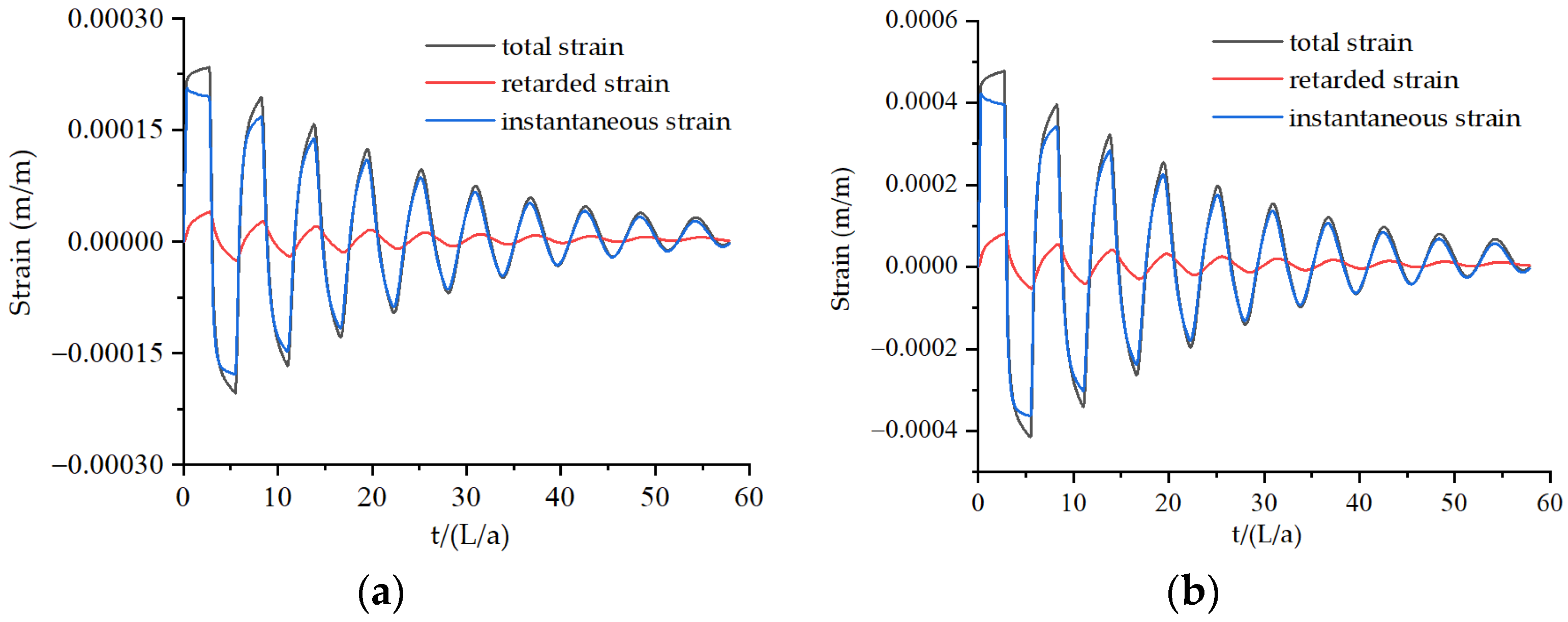
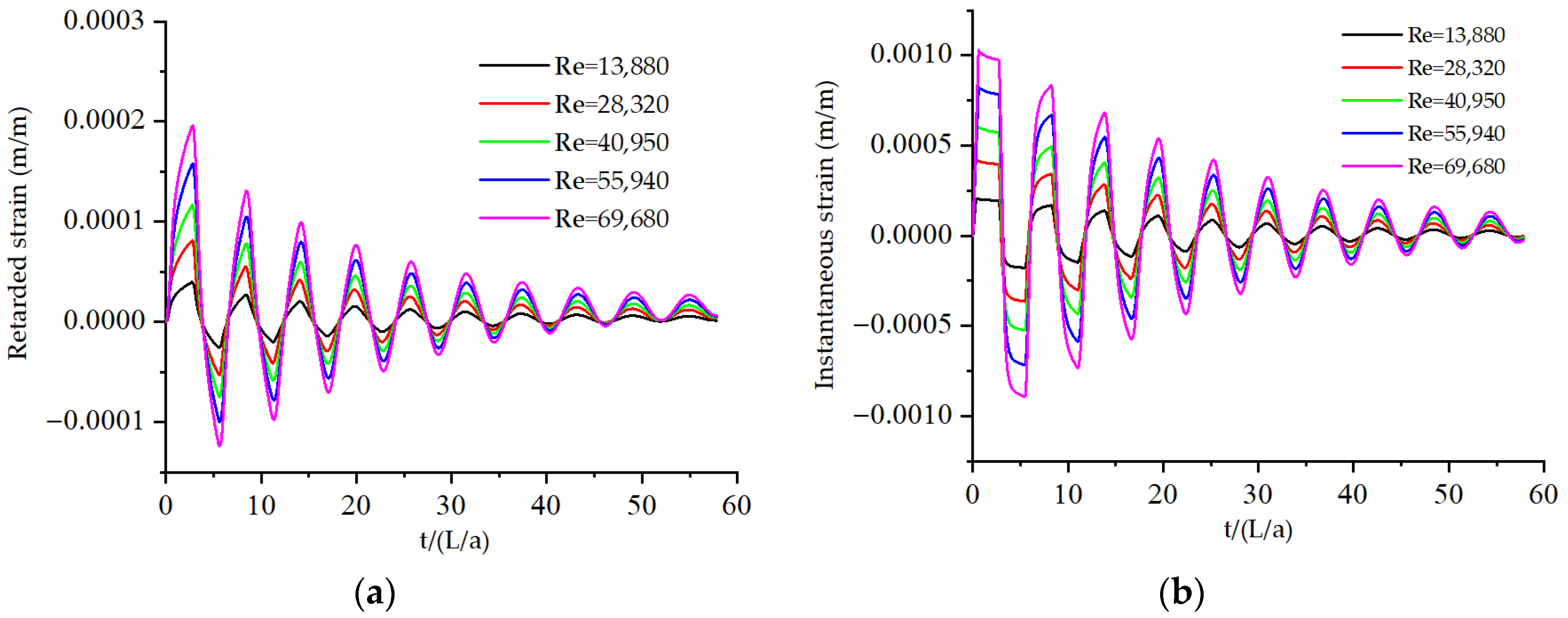
2.2. Kelvin-Voigt Model

The behaviour of the viscoelastic pipes was simulated using the Kelvin-Voight (K-V) model [15,16]. Each of the K-V components consists of a spring and sticky pot, representing the instantaneous strain and retarded strain components, respectively. The total creep compliance is given by:
J ( t ) = J 0 + k = 1 N J k ( 1 e t τ k ) ,
where J0 = 1/E0, E0 is the elastic modulus, J k = 1 / E k is the creep compliance of the k-th element, τ k is the retarded time of the k-th element, and E k is the elasticity modulus of the k-th element.
For viscoelastic pipes, the total strain ε is given by the sum of the instantaneous strain (εe) and retarded component (εr):
ε = ε e + ε r .
Using the K-V model with N elements, the retarded strain is the sum of the single-element deformations [3]:
ε r ( t ) = k = 1 N ε r k ( t ) .
The retarded strain is [4]:
ε r ( x , t ) = k = 1 N ε r k ( x , t ) = k = 1 N γ α D 2 e 0 t [ H ( x , t t ) H 0 ( x ) ] J k τ k e t τ k d t ,
where t’ is the time variation.
The retarded strain rate is algebraically expressed as [17,18]:
ε r ( t ) t = k = 1 N ε r k ( t ) t = k = 1 N ( A H V E ) ,
with
V E = B H 0 + ( A B ) H ( x , t Δ t ) + C ε r k ( x , t Δ t ) ,
A = α D 2 e γ J k Δ t ( 1 e Δ t τ k ) , B = α D 2 e γ J k Δ t e Δ t τ k , C = e Δ t τ k T k ,
where γ is the bulk weight, α is the constraint coefficient, D is the pipe diameter, e is the wall thickness, H is the pressure head, and Δ t = L / ( a × N x ) . Here, N x is the number of pipe meshes.

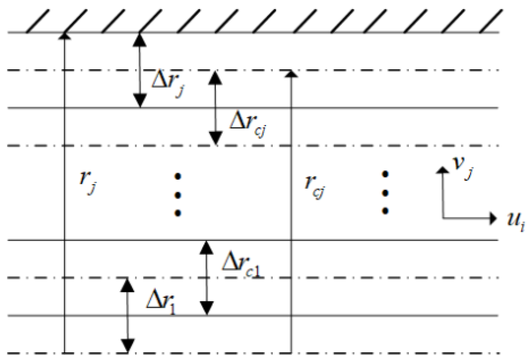
2.3. Numerical Scheme of 1D and Quasi-2D Models

The solutions for transient flows in viscoelastic pipes were calculated by quasi-2D and corresponding 1D models using the method of characteristics (MOC). The characteristic forms of the quasi-2D and corresponding 1D transient-flow equations are:
d H d t ± a g d u d t + a 2 g r ( r v ) r a g 1 ρ r ( r τ ) r + 2 a 2 g k = 1 N ( A H V E ) = 0 ,
d H d t ± a g d Q d t ± a 2 g 4 τ w ρ D + 2 a 2 g k = 1 N ( A H V E ) = 0 .
Because of the steep radial velocity gradient, a gradually encrypted radial grid was applied from the pipe centre to the pipe wall. This is shown in Figure 1, where j is the subscript representing the radial grid number, rj is the radial distance between the outer surface of cylinder j and the pipe centre, and rcj is the radial distance between the centre of cylinder j and the pipe centre.
Integrating Equation (11) on the characteristic lines between times nΔt and (n + 1)Δt (Figure 1) results in the following discretised expressions:
( 1 + F ) H i n + 1 θ C q , j q i , j 1 n + 1 + θ C q , j q i , j n + 1 ω C u 1 , j u i , j 1 n + 1 + ( a g + ω C u 2 , j ) u i , j n + 1 ω C u 3 , j u i , j + 1 n + 1 = K p i , j ,
( 1 + F ) H i n + 1 θ C q , j q i , j 1 n + 1 + θ C q , j q i , j n + 1 + ω C u 1 , j u i , j 1 n + 1 ( a g + ω C u 2 , j ) u i , j n + 1 + ω C u 3 , j u i , j + 1 n + 1 = K n i , j ,
with
F = 2 a 2 Δ t g k = 1 N α D 2 e γ J k Δ t e Δ t / τ k ,
K p i , j = H i 1 n + ( 1 θ ) C q j ( q i 1 , j 1 n q i 1 , j n ) + ( 1 ε ) C u 1 , j u i 1 , j 1 n
+ [ a / g ( 1 ε ) C u 2 , j ] u i 1 , j n + ( 1 ε ) C u 3 , j u i 1 , j + 1 n + 2 a 2 Δ t g k = 1 N V E   ,
K n i , j = H i + 1 n + ( 1 θ ) C q j ( q i + 1 , j 1 n q i + 1 , j n ) ( 1 ε ) C u 1 , j u i + 1 , j 1 n
[ a g ( 1 ε ) C u 2 , j ] u i + 1 , j n ( 1 ε ) C u 3 , j u i + 1 , j + 1 n + 2 a 2 Δ t g k = 1 N V E   ,
C q j = a Δ t 2 g r c j ( r j r j 1 ) ,   C u 1 , j = a Δ t v T j 1 r j 1 g r c j ( r c j r c j 1 ) ( r j r j 1 )   ,
C u 3 , j = a Δ t v T j r j g r c j ( r c j + 1 r c j ) ( r j r j 1 ) ,   C u 2 , j = C u 1 , j + C u 3 , j ,
where ε and θ are the weighting coefficients, q(=rv) is the radial flux, and the source terms Kpi,j, and Kni,j are known values, the elements of which depend on H, u, and q at the previous time level.
When Equation (14) is subtracted from Equation (15), we obtain:
ω C u 1 , j u i , j 1 n + 1 ( a g + ω C u 2 , j ) u i , j n + 1 + ω C u 3 , j u i , j + 1 n + 1 = 0.5 ( K n i , j K p i , j ) .
Instead, if they are added, we obtain:
( 1 + F ) H i n + 1 θ C q , j q i , j 1 n + 1 + θ C q , j q i , j n + 1 = 0.5 ( K n i , j + K p i , j ) .
These equations enable us to calculate the axial velocity, nodal pressure head, and radial flux.
Integrating Equation (12) on the characteristic lines between times nΔt and (n + 1)Δt, the discretised forms of the 1D characteristic equations are expressed as:
( 1 + F ) H i n + 1 + B Q i n + 1 + 4 ε a Δ t ρ g D τ w , i n + 1 = C p ,
( 1 + F ) H i n + 1 B Q i n + 1 4 ε a Δ t ρ g D τ w , i n + 1 = C m   ,
with
τ w , i n + 1 = ρ v T u i , N R + 1 n + 1 Δ r c N r + 1 = ρ v T u i , N R + 1 n + 1 ( D / 2 r c N r + 1 )
C p = H i 1 n + a g A Q i 1 n 4 a Δ t ρ g D τ w , i 1 n + 2 a 2 Δ t g k = 1 N V E ,
C m = H i + 1 n a g A Q i + 1 n + 4 a Δ t ρ g D τ w , i + 1 n + 2 a 2 Δ t g k = 1 N V E   .
A five-region turbulent flow model can be introduced to calculate the turbulent eddy viscosity ( v T ). Combining Equations (21) and (22), the pressure head and discharge may be obtained as:
H i n + 1 = C p + C m 2 ( 1 + F ) ,
Q i n + 1 = C p C m 2 B 4 ε a Δ t ρ g D B τ w i n + 1 .

2.4. ITE Method Based on Quasi-2D Friction Model

The energy equation corresponding to the quasi-2D model is obtained by integrating the basic differential equation. However, in addition to axial flow, radial flow is considered in the quasi-2D model; therefore, radial integration should be considered when the equation associated with the flow rate is integrated [10].
0 L 0 D / 2 [ E q .   ( 3 ) × ρ 2 g H ] d r d x ; 0 L 0 D / 2 [ E q .   ( 4 ) × u ] d r d x
The energy equation of the quasi-2D model is as follows (a detailed derivation is provided in Appendix A):
d U d t + d T d t + D f + W E + W P = 0 ,
where U is the total internal energy of the system, T is the total kinetic energy of the system, Df is the total rate of frictional dissipation, WE is the total rate of work from the ends of the pipe, and WP is the total rate of work from the pipe wall, expressed as follows:
U = ρ g 2 A 2 a 2 0 L H 2 ( x , t ) d x ,
T ( t ) = π ρ D 4 0 L 0 D / 2 u 2 d r d x ,
D f ( t ) = π D 2 0 L 0 D / 2 u r ( r τ ) r d r d x ,
W E = π ρ D g 2 0 D / 2 [ u ( L , t ) H ( L , t ) u ( 0 , t ) H ( 0 , t ) ] d r ,
W P = 2 ρ A g 0 L H ε t d x .

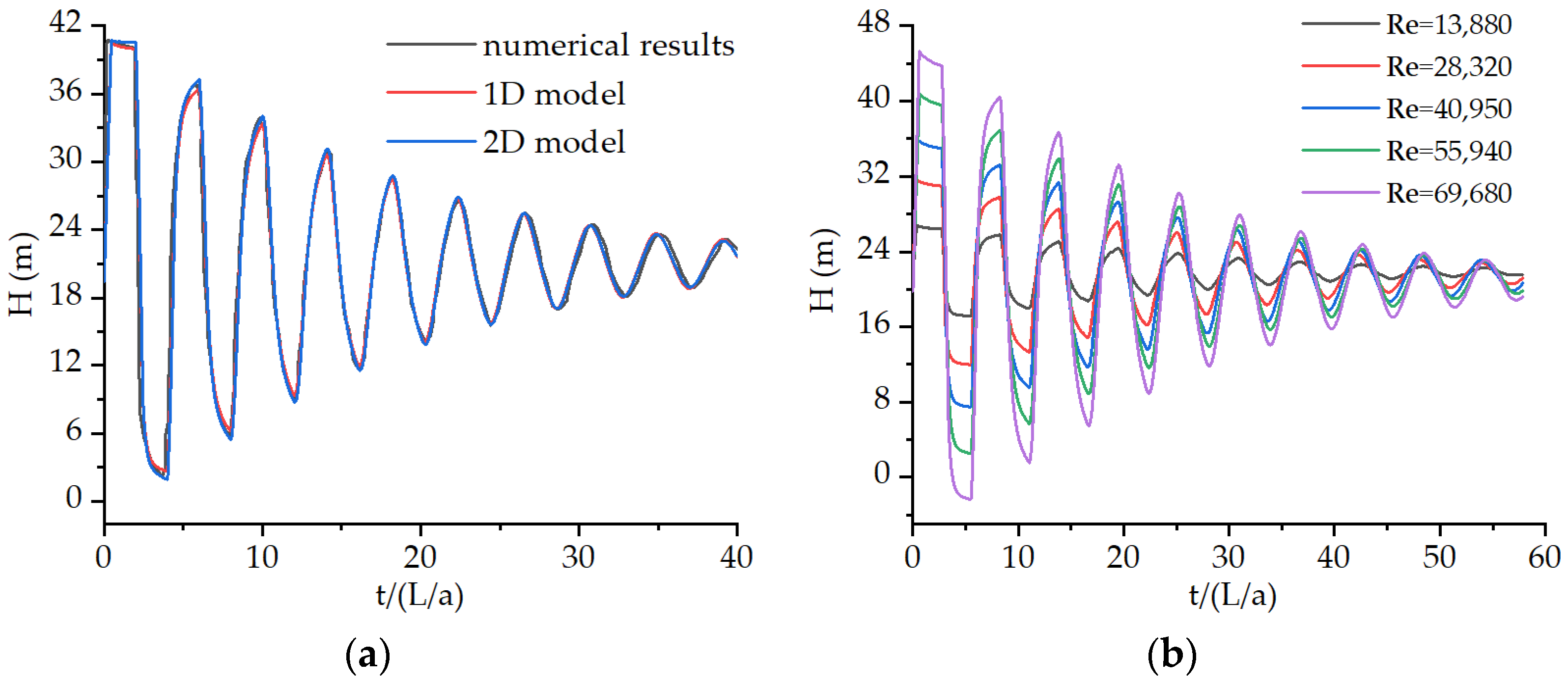
3. Results: Experimental Setup and Validation

The experimental data in this study were obtained from the Water Engineering Laboratory at the University of Perugia, Italy [19]. High-density polyethylene (HDPE) pipe was used in the experiment. A pressure tank was used to maintain the pressure upstream of the pipes, and a fast-closing pneumatic valve was used to generate excitation of the transient flow downstream of the pipes. The inner diameter (D) of the pipe was 93.3 mm, and the wall thickness (e) was 8.1 mm. The length of the experimental pipes (L) used in this study was 128.6 m.
Five groups of experimental data, each with a different Re, initial flow rate, and initial pressure, were analysed in this study. The specific experimental parameters are listed in Table 1. The limiting coefficient of the pipe was 0.97, and the relative roughness of the pipe was 8.57 × 10⁻⁴. The K-V parameters were calibrated according to literature [19], and their values were as follows: 1D model (E0 = 1556 N/mm2, E1 = 7820 N/mm2, τ 1 = 582.6 ms, E2 = 18,370 N/mm2, τ 2 = 59.76 ms, E3 = 6842 N/mm2, and τ 3 = 21,570 ms); 2D model (E0 = 1563 N/mm2, E1 = 9596 N/mm2, τ 1 = 562.3 ms, E2 = 19,490 N/mm2, τ 2 = 52.18 ms, E3 = 5834 N/mm2, and τ 3 = 19,680 ms).
The numerical results of the 1D and quasi-2D models at Re = 55,940 are compared to the experimental results in Figure 2a. The figure shows that the simulation results of the quasi-2D model are very close to the experimental results in terms of peak value, valley value, and phase, especially in the second half-circle of transient flow (30–50 L/a); the same is true for the 1D model. Figure 2b shows the simulation results for the pressure head at different Re values, in which the peak pressure increases with Re. The pressure head decreases with the increase of Reynolds number, whereas the phase is unchanged at different Reynolds numbers.
Figure 3 shows the variation trend of the total, retarded, and instantaneous strain in the two cases. In the critical region of transient flow, the retarded strain accounted for a much smaller proportion of the total strain than the instantaneous strain. Although the retarded strain was relatively small, it can be seen from Figure 3 that, with an increase in L/a, the retarded strain decreased further and the instantaneous strain also showed a decreasing trend. At the later stage of transient flow (30 L/a), the total and instantaneous strain overlapped substantially.
From Figure 3, it can also be seen that the instantaneous strain reached its maximum value at the initial moment of the transient flow, whereas the retarded strain reached its maximum value in the third phase of transient flow (3 L/a); thus, the total strain reached its maximum value at 3 L/a. This suggests that the pressure fluctuation in viscoelastic pipes exhibits a delay compared with that in elastic pipes.
Figure 4 depicts the changes in the instantaneous and retarded strains at five Re values. Both tended to increase with Re. At the same time, there was a little effect on the peak value of the retarded strain at different Re values. The maximum peak values of the instantaneous and retarded strains changed almost linearly with Re. At the same Re value, the maximum instantaneous strain was approximately five times the maximum retarded strain.
Figure 5 illustrates the time difference ( Δ t ) between the extreme value (peak no.) of retarded strain and instantaneous strain (the time of retarded strain/the time of instantaneous strain). According to the line graph, the time difference is the biggest at the first few peak numbers of the Re values, whereas it is closer at the end peak number. This means that different Reynolds numbers have greater influence on the first few cycles of strain, that is, viscoelasticity is obvious in the early phase of transient flow. During the whole period of transient flow, the time difference between retarded strain and instantaneous strain not only shows an upward trend with the peak number monotonic increasing but increases as Re values increase. It would be expected that the retarded strain effect would become smaller with time because the velocity decreases with time; and the difference of Re values also affects viscoelasticity during the transient flow, though not greatly.
To further illustrate the viscoelastic effect, the ratio of retarded strain to total strain ( ε r / ε ) is shown in Figure 6. As can be seen in the line graph, the ratio at the valley decreases from 0.12 in the first valley to 0.05 in the last valley, whereas there is a minor fluctuation in this peak numbers (from 0.175 in the first peak to 0.125 in the last peak, but the smallest value is 0.11 in the five peak). The ratios are consistent at different Re values, which means that the viscoelastic term has no significant effect on transient flow at different Reynolds numbers.

4. Discussion: Energy Analysis at Different Reynolds Numbers

To understand the influence of different Re values on the energy variations of viscoelastic pipes, distinctions between the viscoelasticity and friction terms were analysed.

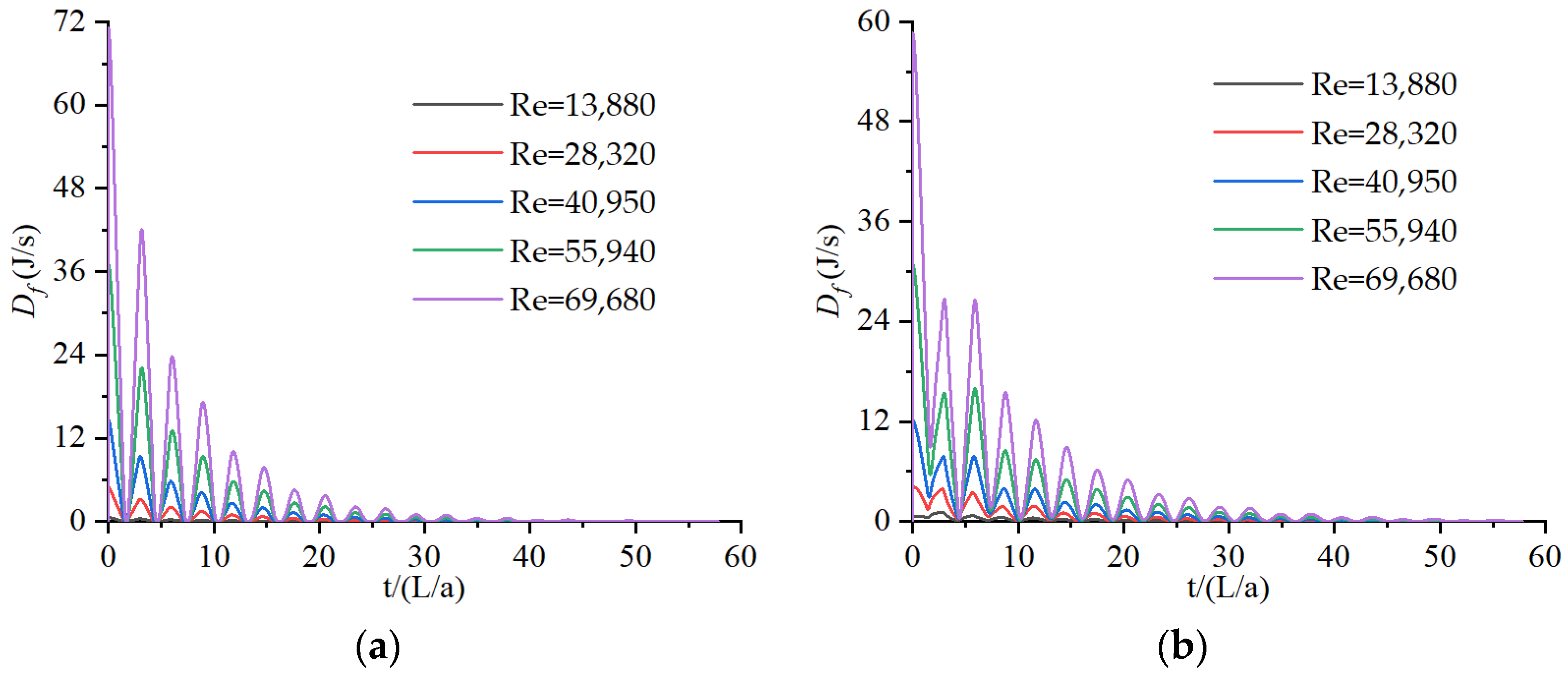
4.1. Df in 1D and 2D Models

The energy changes in the viscoelastic and friction terms of the 1D and 2D friction models under different initial Re values were further analysed based on the ITE method (i.e., Equation (29)). Combined with Equation (33), the simulation results of the work done by the friction term Df are shown in Figure 7. The results show that larger Df values correspond to greater values of the cumulative sum of the wall-shear stress of the entire pipeline. This indicates that the work done by the friction term becomes larger as Re values increase.
In Figure 7a,b, the Df values calculated using the 2D model are larger than those calculated using the 1D model. It can be seen that the 1D model underestimated the instantaneous wall shear stress under flow conditions with initial Re values in the range of 1.0 × 10⁵–3.0 × 10⁵.
As shown in Figure 7, with an increase in the initial Re, Df differed only slightly between the 1D and 2D models. This means that the instantaneous wall-shear stress calculated by the 1D model was close to that calculated by the 2D model, with an initial Re value of 4.0 × 10⁵–7.0 × 10⁵.
For all Re values, Df was maximal near the initial time and gradually decayed with time in both the 2D and 1D models.
Furthermore, the Df values were positive for both models in the critical region of turbulence. Thus, the Df values show the dissipation of the friction energy in the transient flow. This is consistent with the description of transient flow energy in pipelines [10]. The Df values also increased with an increasing initial Re.

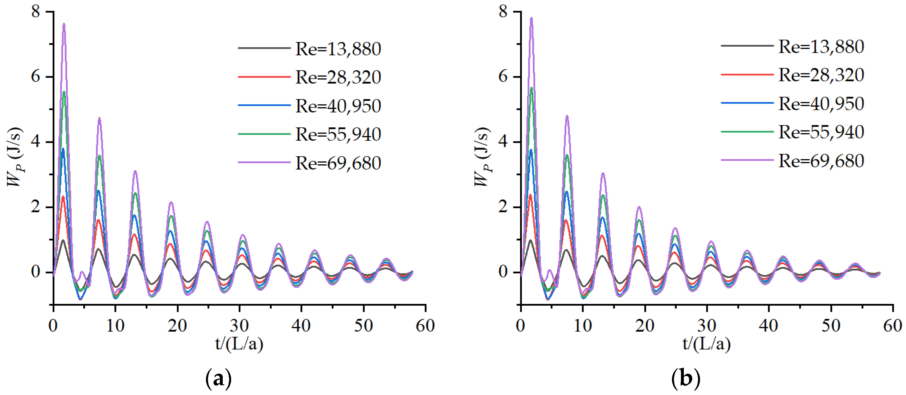
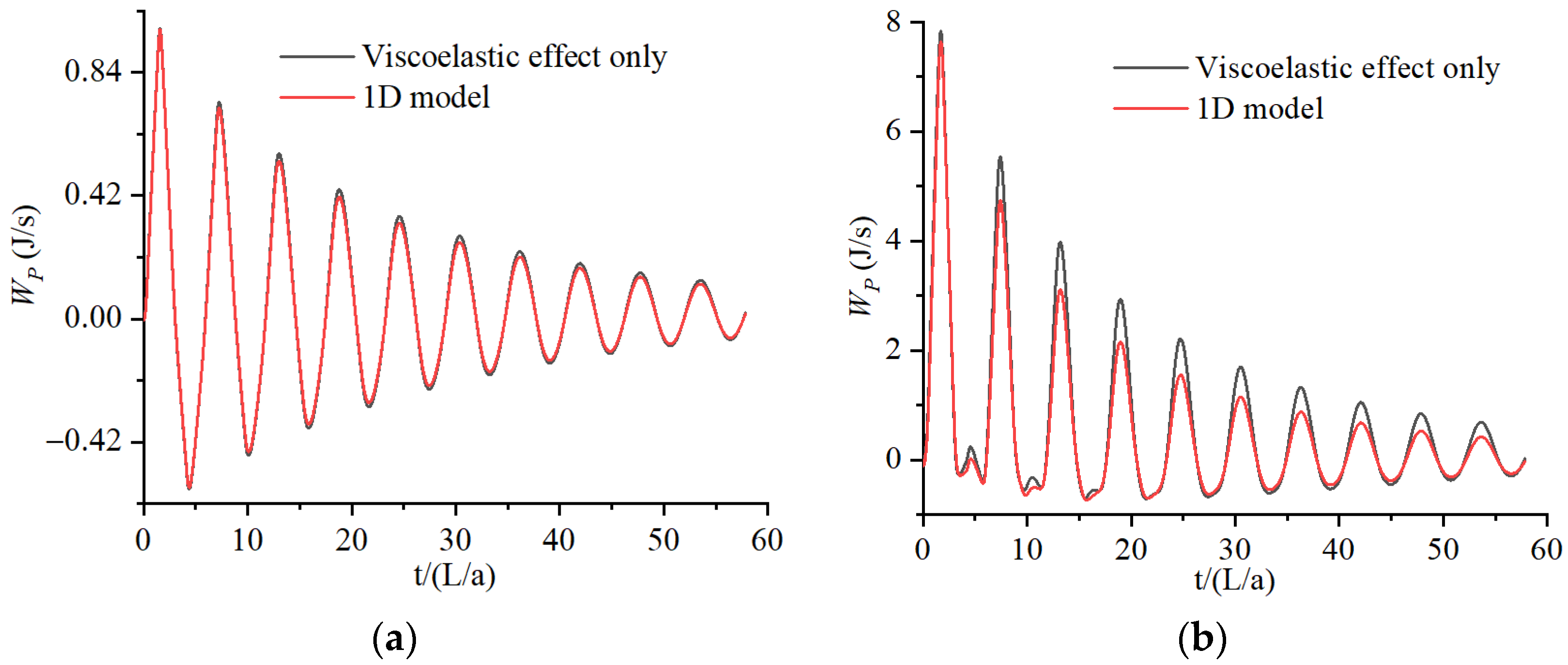
4.2. WP in 1D and 2D Models

The simulation results for WP (the work done by the viscoelastic term of the pipe wall per unit time) are shown in Figure 8. The WP values gradually increased with the initial Re values.
The WP values from the 1D model were similar at all Re values to those from the 2D model because the governing equations of both models were consistent in calculating the retarded strain. The work due to the viscoelastic term of the pipe wall in the two friction models was essentially the same under different initial Re values. In particular, the maximum value of WP calculated by both friction models appeared at approximately 2 L/a for all Re values, and the WP values gradually decayed over time. In the critical region of turbulence, WP had both positive and negative values. This indicates that the interaction between the fluid and the pipe wall during transient flow involves both energy transfer and energy dissipation, which agrees with the description of the energy variation of transient flows in pipelines in the literature [10].
By comparing Figure 7 and Figure 8, it can be seen that the work done by the viscoelastic and friction terms was similar at low Re. With an increase in the initial Re, Df became significantly greater than WP. This shows that the work done by the friction term had a significant influence on the energy dissipation when the initial Re values were relatively high [13].
To further illustrate the dependence of the viscoelastic effect at different flow conditions, the WP values of viscoelastic term were compared with the 1D model at different Reynolds number (Figure 9). From these figures, the difference of WP values between 1D model considering both friction and viscoelastic effects, and only considering the viscoelastic effect, increase with Re values, but compared with the increase of Df values at different Reynolds number, there was a slight increase in WP values in orders of magnitude. This is because the viscoelastic effect does not dominate under different initial Reynolds numbers [10,20].

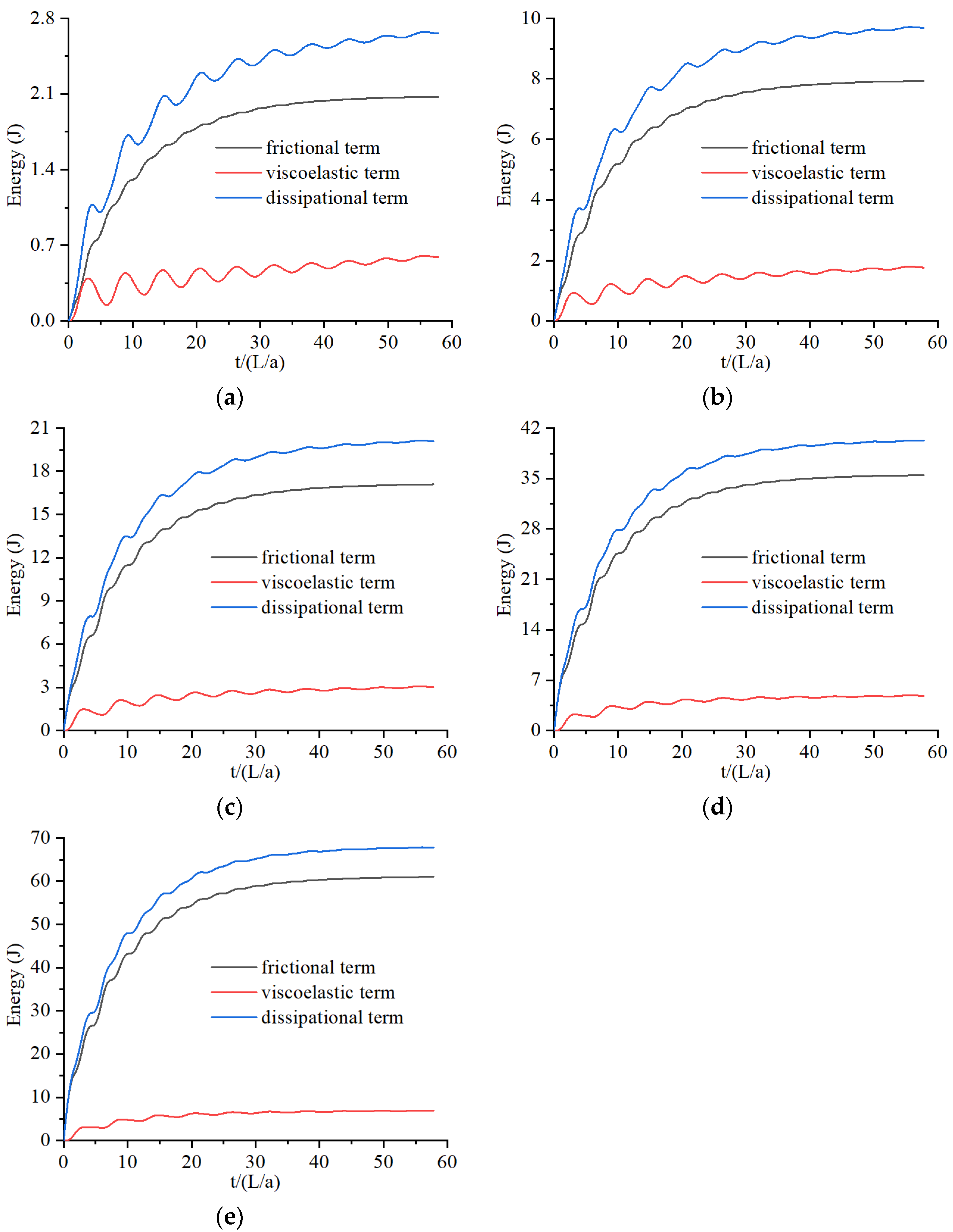
4.3. Energy integral in 2D Models

Figure 10 shows the cumulative energies of the viscoelastic and friction terms, along with their sum (the total dissipational energy change) for the entire pipeline under different initial Re values.
The cumulative work done by the friction term increased with time, most steeply between 0 and 5 L/a; after 20 L/a, the energy dissipation gradually stabilised. This indicates that energy dissipation was the dominant mode of energy change.
The positive energy change of the viscoelastic term was the largest between 0 and 2.5 L/a, and the negative energy change was largest between 2.5 and 5 L/a, as shown in Figure 10. The energy change in the viscoelastic term had a sinusoidal fluctuation and an overall upward trend over time. This indicates that the energy change between the viscoelastic pipes and the fluid in the pipe not only led to energy conversion but also energy dissipation in the initial stage of the transient flow in the pipes. The energy changes became predominantly dissipative as time elapsed.
It can also be seen from Figure 10 that the energy changes of both the viscoelastic and friction terms increased with Re. At different initial Re values, the energy variation trend of the friction term was essentially the same. However, for the energy change of the viscoelastic term, the fluctuation range was larger and the duration longer when the initial Re values were small.
In particular, the proportion of energy dissipation generated by the friction term in the total energy change increased continuously with an increase in the initial Re values. Accordingly, the proportion of energy change generated by the viscoelastic term in the total energy change decreased. More specifically, the proportions of the viscoelastic terms in the total energy variation were 22.1% (Re = 13,880), 18.2% (Re = 28,320), 15.1% (Re = 40,950), 11.9% (Re = 55,940), and 10.1% (Re = 69,680) when the transient flow time was approximately 60 L/a.

5. Conclusions

In this study, the ITE method was used to derive the energy equation of a quasi-2D model of viscoelastic pipes, and the work changes of the friction term and viscoelastic term in 1D and 2D models under different initial Re values were compared. The results are as follows:
(1) When the initial Re was < 3.0 × 10⁵, the 1D (but not the 2D) model underestimated the work due to the friction term Df. For Re > 3.0 × 10⁵, this error was reduced.
(2) The work done by the viscoelastic term of the pipe wall remained approximately constant under different initial Re values for both the 1D and 2D models.
(3) With an increase in Re values, both the viscoelastic and frictional work in the 1D and 2D models increased with time. However, Df > WP for a large initial Re.
(4) The energy dissipation of the friction term increased significantly initially then slowed down, and finally approached a constant value.
(5) The energy change of the viscoelastic term exhibited sinusoidal fluctuation during the early stage of the transient flow. At a smaller initial Re, the fluctuation in energy lasted for a long time, presented an overall upward trend, and finally approached a constant value.
(6) With an increase in initial Re values, the proportion of the energy dissipation generated by the friction term in the total energy change increased continuously, whereas the proportion of the energy change generated by the viscoelastic term in the total energy change decreased correspondingly.

Author Contributions

Conceptualization, K.W. and Y.F.; methodology, Y.X.; software, H.L.; validation, G.L., Y.F. and Y.X.; formal analysis, K.W.; investigation, G.L.; resources, Y.F.; data curation, H.L.; writing—original draft preparation, K.W.; writing—review and editing, Y.X.; visualization, Y.F.; supervision, Y.F.; project administration, Y.X.; funding acquisition, Y.X. All authors have read and agreed to the published version of the manuscript.

Funding

This research was funded by the National Natural Science Foundation of China (Grant No. 51978202), the Science Foundation of Harbin University of Commerce (2020CX07), and the Natural Science Fund of Heilongjiang Province (LH2019E111 and LH2020E028).

Data Availability Statement

All relevant data are included in the paper. The data presented in this study are available on request from the corresponding author.

Conflicts of Interest

The authors declare no conflict of interest.

Nomenclature

The following symbols are used in this paper:
Across-sectional area of the pipeline
awave speed
Dpipe diameter
Dftotal rate of frictional dissipation
E k elasticity modulus of the k-th element
ewall thickness
ggravitational acceleration
Hpressure head
Jcreep compliance of the k-th element
jsubscript representing the radial grid number
Nrnumber of segments along the radius
Nr0number of cylinders along the radius
Qdischarge
qradial flux
rradial distance from the pipe centre
rcjradial distance between the centre of the cylinder j cross-section and the pipe centre
rjradial distance between the outer surface of the cylinder j cross-section and the pipe centre
Ttotal kinetic energy of the system
ttime
Utotal internal energy of the system
ulongitudinal velocity
vradial velocity
WEtotal rate of work from the ends of the pipe
WPtotal rate of work from the pipe wall
xaxial coordinate along the pipe
Greek Symbols
α constraint coefficient
ε, θweighting coefficients
ε r retarded strain
ρ density
τ shear stress
τ k retarded time of the k-th element
τ w pipe-wall shear stress
γ bulk weight
Abbreviations
quasi-2Dquasi-two-dimensional
1Done-dimensional
ReReynolds number
K-VKelvin-Voight
HDPEhigh-density polyethylene pipe
MOCmethod of characteristics

Appendix A. Derivation of Equation (29)

We multiply Equation (3) by Hdx and integrate along the pipe length L:
g 2 a 2 d d t 0 L H 2 d x + 0 L H u x d x + 2 0 L H ε t d x = 0
Then, we integrate along the pipe diameter D:
g 2 a 2 d d t 0 D / 2 0 L H 2 d x d r + 0 D / 2 0 L H u x d x d r + 2 0 D / 2 0 L H ε t d x d r = 0
In the quasi-2D model, the pressure changes are only along the axial direction of the pipeline, and slight changes in the radial direction are ignored. Therefore, the first and third terms in Equation (A2) can be treated as constants in the pipeline radial direction:
g 2 a 2 D 2 d d t 0 L H 2 d x + 0 L 0 D / 2 H u x d r d x + 2 D 2 0 L H ε t d x = 0
Multiplying by 2ρAg/D, we have
ρ A g 2 2 a 2 d d t 0 L H 2 d x + π ρ D g 2 0 L 0 D / 2 H u x d r d x + 2 ρ A g 0 L H ε t d x = 0
Next, we multiply Equation (2) by u and integrate along the pipe diameter D and the pipe length L simultaneously:
1 2 d d t 0 L 0 D / 2 u 2 d r d x + g 0 L 0 D / 2 u H x d r d x 1 ρ 0 L 0 D / 2 u r ( r τ ) r d r d x = 0
Calculating the derivatives of the second term of Equation (A5), we have
0 D / 2 0 L u H x d x d r = 0 D / 2 [ 0 L H u x d x + u ( L , t ) H ( L , t ) u ( 0 , t ) H ( 0 , t ) ] d r
Solving Equations (A4) and (A6) simultaneously yields
ρ A g 2 2 a 2 d d t 0 L H 2 d x π ρ D g 2 0 D / 2 0 L u H x d x d r + 2 ρ A g 0 L H ε t d x + π ρ D g 2 0 D / 2 [ u ( L , t ) H ( L , t ) u ( 0 , t ) H ( 0 , t ) ] d r = 0
Finally, solving Equations (A5) and (A7) simultaneously yields:
ρ A g 2 2 a 2 d d t 0 L H 2 d x + π ρ D 4 d d t 0 L 0 D / 2 u 2 d r d x π D 2 0 L 0 D / 2 u r ( r τ ) r d r d x + 2 ρ A g 0 L H ε t d x + π ρ D g 2 0 D / 2 [ u ( L , t ) H ( L , t ) u ( 0 , t ) H ( 0 , t ) ] d r = 0

References

  1. Duan, H.F.; Pan, B.; Wang, M.L.; Chen, L.; Zheng, F.; Zhang, Y. State-of-the-art review on the transient flow modeling and utilization for urban water supply system (UWSS) management. J. Water Supply Res. Technol. 2020, 69, 858–893. [Google Scholar] [CrossRef]
  2. Rieutord, E.; Blanchard, A. Pulsating viscoelastic pipe flow–water-hammer. J. Hydraul. Res. 1979, 17, 217–229. [Google Scholar] [CrossRef]
  3. Covas, D.; Stoianov, I.; Mano, J.F.; Ramos, H.; Graham, N.; Maksimovic, C. The dynamic effect of pipe-wall visco-elasticity in hydraulic transients. Part I: Experimental analysis and creep characterization. J. Hydraul. Res. 2004, 42, 516–530. [Google Scholar] [CrossRef]
  4. Covas, D.; Stoianov, I.; Mano, J.F.; Ramos, H.; Graham, N.; Maksimovic, C. The dynamic effect of pipe-wall viscoelasticity in hydraulic transients. Part II: Model development, calibration and verification. J. Hydraul. Res. 2005, 43, 56–70. [Google Scholar] [CrossRef]
  5. Urbanowicz, K. Analytical expressions for effective weighting functions used during simulations of water hammer. J. Theor. Appl. Mech. 2017, 55, 1029–1040. [Google Scholar] [CrossRef] [Green Version]
  6. Pezzinga, G. Quasi-2D model for unsteady flow in pipe networks. J. Hydraul. Eng. 1999, 125, 676–685. [Google Scholar] [CrossRef]
  7. Firkowski, M.; Urbanowicz, K.; Duan, H.F. Simulation of unsteady flow in viscoelastic pipes. SN Appl. Sci. 2019, 1, 519. [Google Scholar] [CrossRef] [Green Version]
  8. Urbanowicz, K.; Duan, H.F.; Bergant, A. Transient liquid flow in plastic pipes. J. Mech. Eng. 2020, 66, 77–90. [Google Scholar] [CrossRef]
  9. Sun, Q.; Zhang, Z.; Wu, Y.; Xu, Y.; Liang, H. Numerical analysis of transient pressure damping in viscoelastic pipes at different water temperatures. Materials 2022, 15, 4904. [Google Scholar] [CrossRef]
  10. Duan, H.F.; Ghidaoui, M.S.; Lee, P.J.; Tung, Y.-K. Energy analysis of viscoelasticity effects in pipe fluid transients. J. Appl. Mech. 2010, 77, 044503.1–044503.5. [Google Scholar] [CrossRef]
  11. Karney, B.W. Energy relations in transient closed-conduit flow. J. Hydraul. Eng. 1990, 116, 1180–1196. [Google Scholar] [CrossRef]
  12. Duan, H.F.; Meniconi, S.; Lee, P.J.; Brunone, B.; Ghidaoui, M.S. Local and integral energy-based evaluation for the unsteady friction relevance in transient pipe flows. J. Hydraul. Eng. 2017, 143, 04017015. [Google Scholar] [CrossRef] [Green Version]
  13. Meniconi, S.; Brunone, B.; Ferrante, M.; Massari, C. Energy dissipation and pressure decay during transients in viscoelastic pipes with an in-line valve. J. Fluids Struct. 2014, 45, 235–249. [Google Scholar] [CrossRef]
  14. Meniconi, S.; Duan, H.F.; Brunone, B.; Ghidaoui, M.S.; Lee, P.J.; Ferrante, M. Further developments in rapidly decelerating turbulent pipe flow modeling. J. Hydraul. Eng. 2014, 140, 04014028. [Google Scholar] [CrossRef] [Green Version]
  15. Riasi, A.; Nourbakhsh, A.; Raisee, M. Energy dissipation in unsteady turbulent pipe flows caused by water hammer. Comput. Fluids 2013, 73, 124–133. [Google Scholar] [CrossRef]
  16. Keramat, A.; Haghighi, A. Straightforward transient-based approach for the creep function determination in viscoelastic pipes. J. Hydraul. Eng. 2014, 140, 04014058. [Google Scholar] [CrossRef]
  17. Gong, J.; Zecchin, A.C.; Lambert, M.F.; Simpson, A.R. Determination of the creep function of viscoelastic pipelines using system resonant frequencies with hydraulic transient analysis. J. Hydraul. Eng. 2016, 142, 04016023. [Google Scholar] [CrossRef] [Green Version]
  18. Urbanowicz, K.; Firkowski, M.; Zarzycki, Z. Modelling water hammer in viscoelastic pipelines: Short brief. J. Phys. Conf. Ser. 2016, 760, 012037. [Google Scholar] [CrossRef]
  19. Pezzinga, G.; Brunone, B.; Meniconi, S. Relevance of pipe period on Kelvin-Voigt viscoelastic parameters: 1D and 2-D inverse transient analysis. J. Hydraul. Eng. 2016, 142, 04016063. [Google Scholar] [CrossRef]
  20. Pan, B.; Duan, H.F.; Meniconi, S.; Urbanowicz, K.; Che, T.C.; Brunone, B. Multistage Frequency-Domain Transient-Based Method for the Analysis of Viscoelastic Parameters of Plastic Pipes. J. Hydraul. Eng. 2020, 146, 04019068. [Google Scholar] [CrossRef]
Figure 1. Radial difference grid.
Water 14 03258 g001
Figure 2. Variation in pressure head with time: (a) results of experiment and two simulations at Re = 55,940; (b) simulation results at different Re values.
Water 14 03258 g002
Figure 3. Results of strain at different Re values: (a) Re = 13,880; (b) Re = 28,320.
Water 14 03258 g003
Figure 4. Variation of (a) retarded and (b) instantaneous strain at different Re values.
Water 14 03258 g004
Figure 5. The time difference between the extreme value of retarded strain and instantaneous strain.
Water 14 03258 g005
Figure 6. Ratio of retarded strain to total strain.
Water 14 03258 g006
Figure 7. Frictional work Df at different Re values in the critical region: (a) 1D model; (b) 2D model.
Water 14 03258 g007
Figure 8. Viscoelastic work, WP, at different Re values in the critical region: (a) 1D model; (b) 2D model.
Water 14 03258 g008
Figure 9. Work done of WP by 1D model including only viscoelastic effect: (a) Re = 13,880; (b) Re = 69,680.
Water 14 03258 g009
Figure 10. Energy variation of 2D model in critical region at different Re values: (a) Re = 13,880; (b) Re = 28,320; (c) Re = 40,950; (d) Re = 55,940; (e) Re = 69,680.
Water 14 03258 g010
Table 1. Experimental settings [19].
CaseQ (L/s)ReH0 (m)Tc (s)
1113,38021.630.0875
22.0428,32021.130.0752
32.9540,95020.740.1188
44.0355,94020.340.1575
55.0269,68019.820.1533
Publisher’s Note: MDPI stays neutral with regard to jurisdictional claims in published maps and institutional affiliations.

